Very High-Resolution Imagery and Machine Learning for Detailed Mapping of Riparian Vegetation and Substrate Types

Abstract

Riparian zones fulfill diverse ecological and economic functions. Sustainable management requires detailed spatial information about vegetation and hydromorphological properties. In this study, we propose a machine learning classification workflow to map classes of the thematic levels Basic surface types (BA), Vegetation units (VE), Dominant stands (DO) and Substrate types (SU) based on multispectral imagery from an unmanned aerial system (UAS). A case study was carried out in Emmericher Ward on the river Rhine, Germany. The results showed that: (I) In terms of overall accuracy, classification results decreased with increasing detail of classes from BA (88.9%) and VE (88.4%) to DO (74.8%) or SU (62%), respectively. (II) The use of Support Vector Machines and Extreme Gradient Boost algorithms did not increase classification performance in comparison to Random Forest. (III) Based on probability maps, classification performance was lower in areas of shaded vegetation and in the transition zones. (IV) In order to cover larger areas, a gyrocopter can be used applying the same workflow and achieving comparable results as by UAS for thematic levels BA, VE and homogeneous classes covering larger areas. The generated classification maps are a valuable tool for ecologically integrated water management.

1. Introduction

Surface waters, their riparian zones and floodplains are hotspots for highly specialized vegetation communities and fulfill valuable ecosystem services. Here, flooding and water availability drive the small-scale distribution of vegetation communities [1]. The interplay of vegetation and sedimentation and erosion processes leads to diverse terrain structures which provide habitats for endangered species [2,3]. Riparian zones perform several functions: they act as natural corridors for terrestrial wildlife, contribute to water purification, reduce flood vulnerability and serve as areas of recreation [4,5]. At the same time, they are often degraded or eliminated by human activities, e.g., due to chemical contamination or flood regulation measures [2,6]. The federal waterways in Germany also act as an efficient and economically indispensable mode of transport, under increased anthropogenic pressure. In order to counteract degradation and to improve the ecological state of rivers while considering all concerned parties and diverse interests, several intergovernmental action plans have been developed [7]. Implementation strategies are defined in several provisions, including the EU Biodiversity Strategy for 2030, EU Fauna and Flora Habitat Directive [8], EU Water Framework Directive [9], and realized within the scope of country specific activities such as Germany’s Blue Belt Program [10].

Waterways and riparian systems are heterogeneous due to their topography, hydrological properties, vegetation and human action [11,12]. Hence, detailed data are crucial for the proper management of those sites. Traditionally, data are collected during field surveys that are time-consuming and whose spatial coverage is often insufficient in larger areas. Due to the complex structure and spatial arrangement of riparian ecosystems, some sites may be difficult to access leading to a lack of information. Remote sensing techniques have since been established as a facilitating and supporting method to gather information about ecosystems. Comprehensive reviews on different approaches using remote sensing methods for mapping riparian ecosystems are given by Huylenbroeck, et al. [13], Piégay, et al. [14] and Tomsett and Leyland [15]. Unmanned aerial systems (UAS) are suitable to obtain images with a resolution in the centimeter range to detect narrow, linear riparian habitats defined by vegetation and sediment types.

The applicability of UAS has been evaluated for multiple purposes in river management and research. For instance, they were used for long-term post-restoration monitoring of an urban stream [16] or to map dominant substrate types of the riverbed [17]. Moreover, UAS have been used to map vegetation types [12,18,19] and vegetation coverage [12], to track the phenological change of natural vegetation [20] or to monitor invasive species [21,22]. Studies focusing on an integrative approach by using the same very high-resolution imagery to retrieve detailed information across multiple disciplines, such as vegetation cover and substrate types, are still sparse.

Management actions, such as restoration, are mostly applied on a local scale in narrow corridors ranging from a few hectares up to kilometers in size [23]. Due to the relatively low flight altitude, UAS are suitable to cover areas of a few hectares [14,24]. Lightweight manned gyrocopters can be an alternative means to acquire imagery with very high spatial resolution in the decimeter range even over larger areas with recording rates of up to 40 km²/h [25]. The gyrocopter is an ultralight rotorcraft that differs from a helicopter in that the wing is not actively propelled by an engine but only by the incoming airflow. This effect is known as autorotation and provides the necessary lift and flight capability. Furthermore, due to the simple design principle compared to helicopters, gyrocopters are significantly cheaper to purchase and operate. The flight characteristics of a gyrocopter are more like those of an airplane than a helicopter, making it much easier to fly. Pilots need an ultralight aircraft pilot license for gyrocopter. They therefore represent an economic alternative to helicopters. In particular, the excellent low-speed flight characteristics and maneuverability make the gyrocopter for observation and survey flights. The gyrocopter flies at an altitude of between 150 m and 3000 m at speeds between 30 km/h and 150 km/h. Considering the possibility of additional payloads and the flexibility of gyrocopters, they have proven to be a suitable tool, for instance, to obtain water temperature data over larger areas in the Elbe estuary [26], to map invasive plant species [27] or to identify European Spruce infested by bark beetles [28]. Hence, gyrocopters might be used to map detailed classes of riparian surface types over larger areas. To our knowledge, there are no studies using gyrocopters to map detailed cover classes of riparian ecosystems.

Dealing with very high-resolution data as acquired with UAS requires sophisticated methods [29]. At the same time, they need to be applicable for regular management [30], where it is essential to use reproducible methods for spatial and temporal comparability. Several studies have shown that approaches using object-based image analysis (OBIA), where areas of homogeneous pixels are grouped into objects, have outperformed pixel-based approaches when classifications are based on very high-resolution data (see, e.g., reviews by Dronova [11] and Mahdavi, et al. [31]). Machine learning algorithms offer various ways to classify these objects. Algorithm performance depends on the classes to be mapped, the training data, and the predictor variables provided, which is why multiple classifiers should be tested to identify the most suitable option [32]. Well-established algorithms for this type of classification are, for instance, Random Forest (RF), showing sufficient results for mapping riparian vegetation [18,33,34]; Support Vector Machine (SVM), which is mentioned to achieve good results even with small sampling sizes [11,35]; and Extreme Gradient Boost (XGBoost), which is a more recent and popular method for classification studies [36,37,38]. A comprehensive overview of machine learning methods for classification tasks is given in the reviews by Fassnacht et al. [35] and Maxwell, Warner and Fang [34]. The assessment of classification maps is generally conducted using a confusion matrix [39]. Additionally, we used spatial distribution of classification accuracy as this information is especially important for management. An easy and straight-forward way to obtain these data are probability maps, e.g., calculated within RF, that provide information on the degree of certainty with which an object is assigned to a given class [40]. Mapping the probability of a classification can identify areas that should be prioritized and assessed more carefully during field campaigns [41].The various aspects of the image classification workflow have to be fine-tuned to produce results with sufficient quality and comparability necessary for management purposes [13].

In this study, we propose an OBIA classification framework based on multispectral UAS imagery for mapping vegetation communities and hydromorphological substrate classes with different levels of detail (later referred to as ‘levels’) in a riparian ecosystem. The study area is a part of the nature conservation area Emmericher Ward located at the river Rhine, Germany. Besides the UAS and gyrocopter imagery and in situ data acquired during the field survey, additional data for the study area were used, including a flood duration model and a digital elevation model based on LiDAR.

The aims of this study are:

(I)

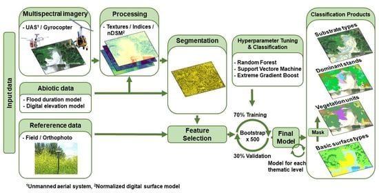
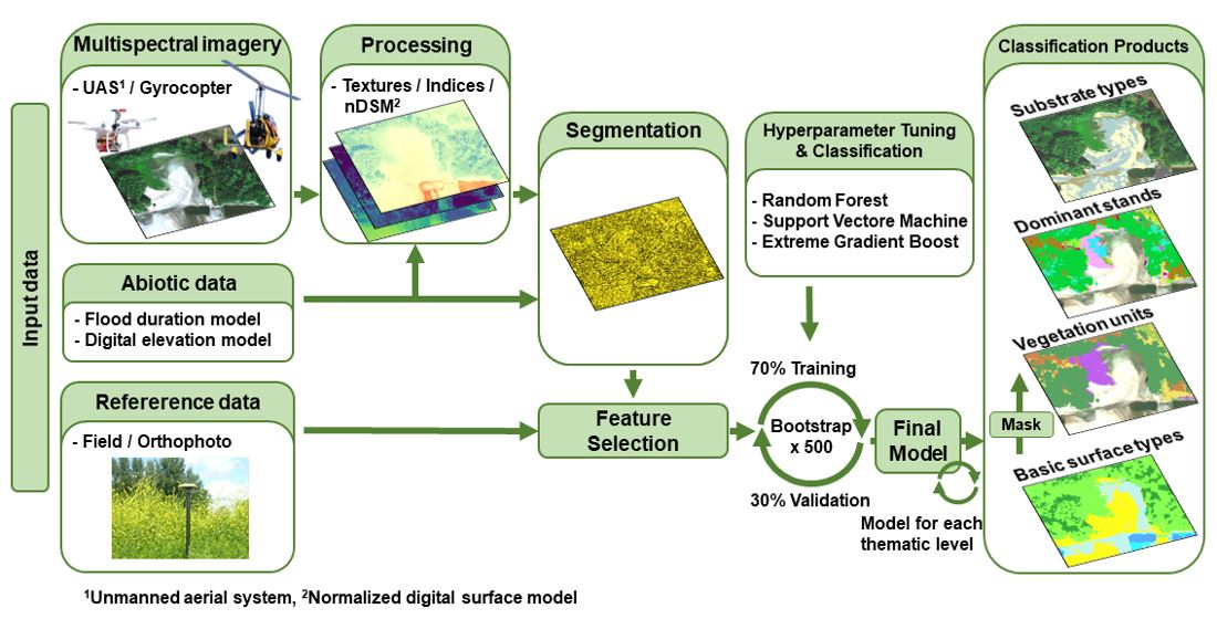
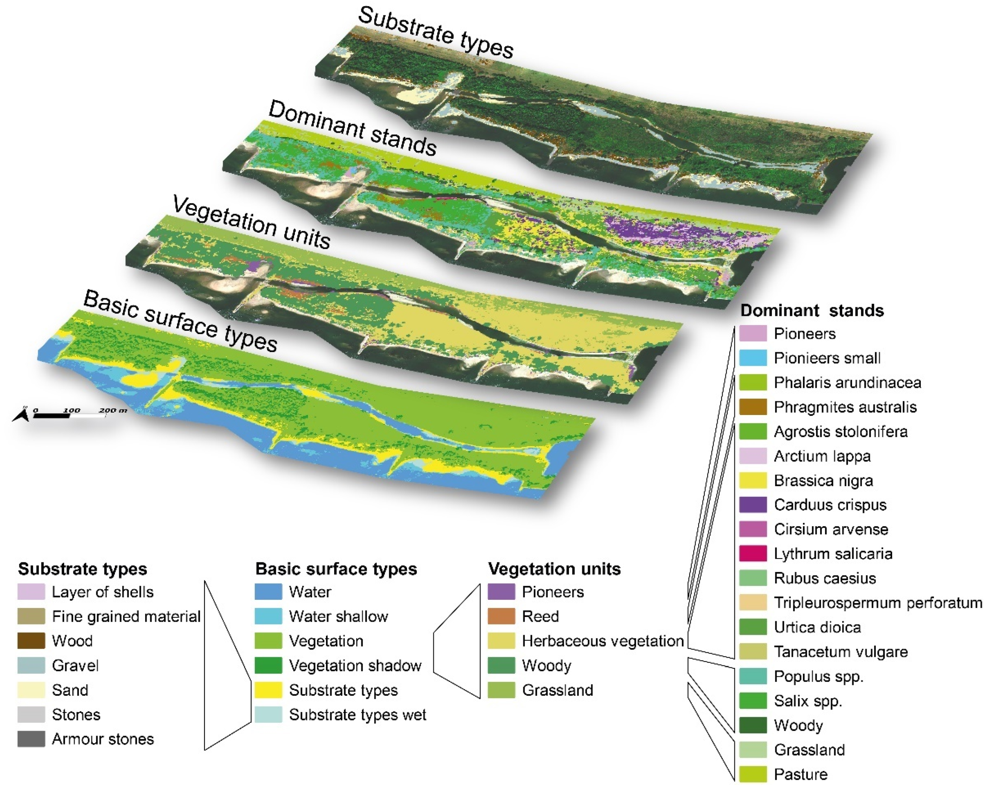
To evaluate the final results for Random Forest classification models for the levels Basic surface type (BA, e.g., substrate types, water), Vegetation units (VE, e.g., reed, herbaceous vegetation), Dominant stands (DO, up to species level) and Substrate types (SU, e.g., sand, gravel);

(II)

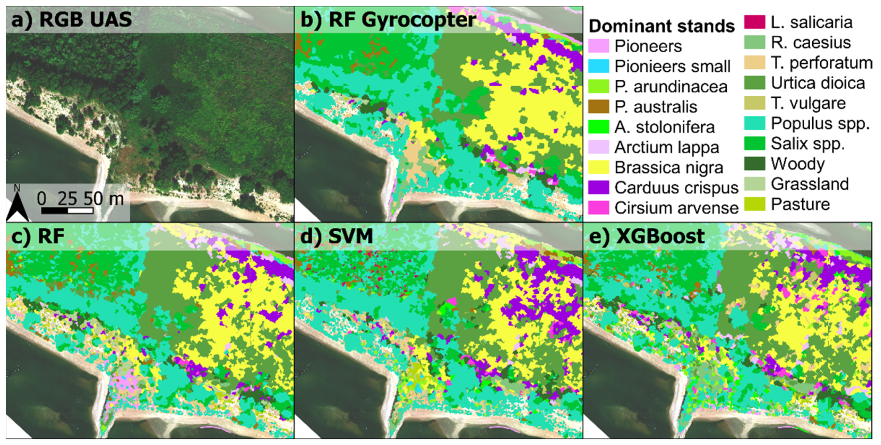
To compare classification results from the Random Forest algorithm (RF) with Support Vector Machine (SVM) and Extreme Gradient Boosting (XGBoost);

(III)

To identify areas in the classification results with high degrees of uncertainty or certainty, respectively; and

(IV)

To transfer the workflow to data acquired by gyrocopter and to compare the achieved results with those from UAS data.

2. Materials and Methods

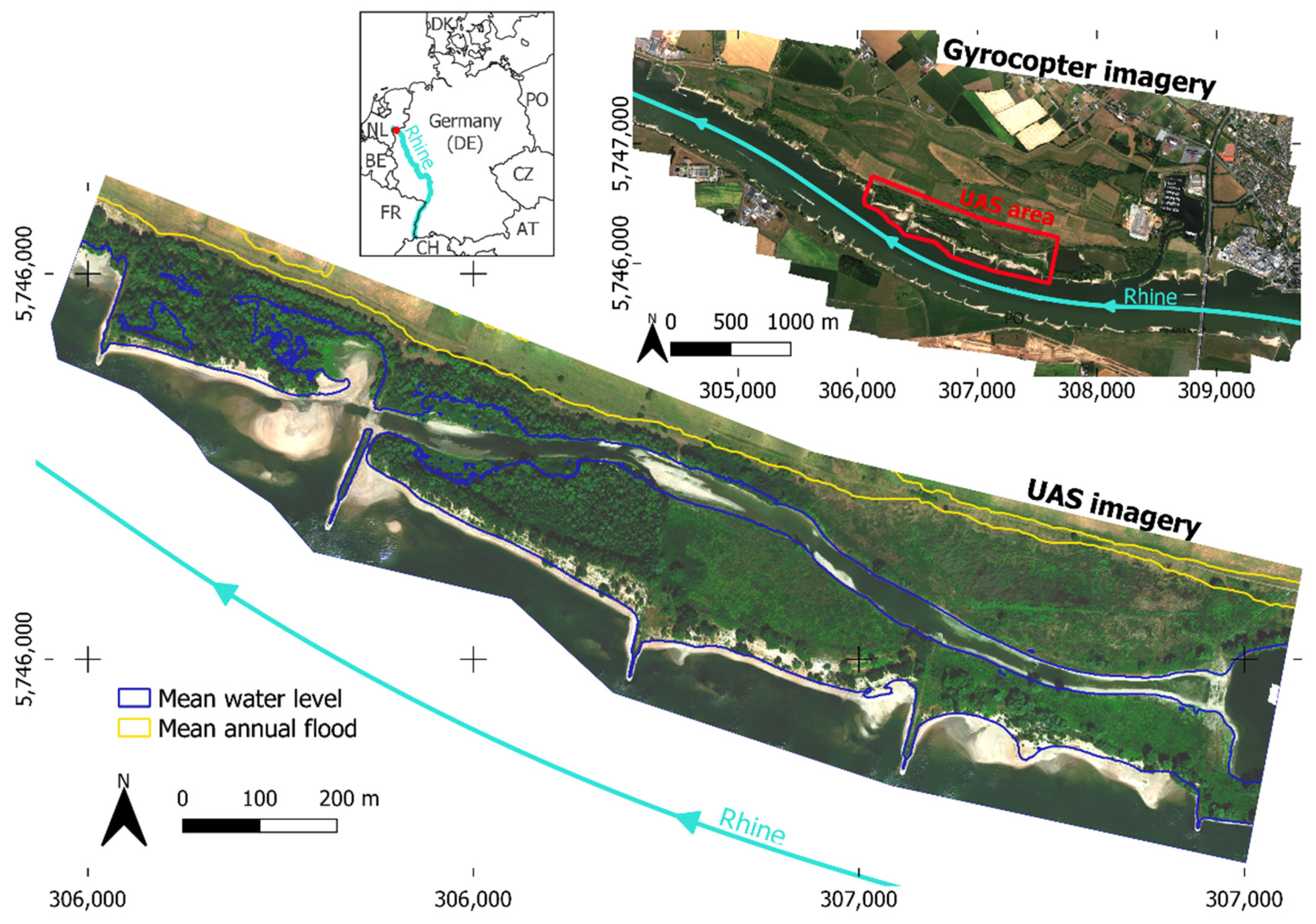
2.1. Study Area

This study was conducted in the nature conservation area Emmericher Ward, situated at the river Rhine in Germany, near the border to the Netherlands (Figure 1). The floodplain Emmericher Ward is part of the Natura 2000 network of breeding and resting sites for rare and threatened species within the framework of the EU Fauna and Flora Habitat Directive [42]. The study area of 59 ha includes a secondary channel, which is connected to the river Rhine, and exhibits high flood dynamics. The mean annual flood (based on a period of 100-year, yellow line in Figure 1) regularly inundates large parts of the study area and reaches the extensively managed grassland in the northern part. Due to this circumstance, the area has a high heterogeneity in vegetation and hydromorphology. The vegetation consists of meadows, softwood floodplain forest, reed, riparian pioneers and stands of herbaceous vegetation. The substrate types are dominated by sand and gravel with typical hydromorphological elements for river habitats, for instance, banks, island areas, scours and shallow water zones.

2.2. Image Data and Pre-Processing

Flight surveys with the UAS and gyrocopter for obtaining multispectral imagery took place in July 2019. In parallel, reference data of vegetation and hydromorphological substrate types were recorded in the field.

UAS imagery was obtained using the MicaSense RedEdge-M camera mounted on a DJI Phantom 4 Pro (

Table 1. Specifications of the sensor systems used and imagery acquired by unmanned aerial system (UAS) and gyrocopter.

Platform	Sensor	Center of Wavebands in nm (Bandwidth in Parenthesis)					Spatial Resolution in cm	Flight Altitude in m
		Blue	Green	Red	Red-Edge	Near-Infrared
UAS (DJI Phantom 4 Pro)	Micasence RedEdge-M	475 (20)	560 (20)	668 (10)	717 (10)	840 (40)	5	70
Gyrocopter	PanX 2.0	475 (50)	550 (50)	650 (25)	_	875 (25)	28	650

). During the flight, images were taken every two seconds, while gain and exposure settings were set to automatic. The raw images are converted to spectral radiance, followed by reflectance with the aid of a calibrated 5-panel greyscale, which was deployed and captured by the camera system in the field during data acquisition. The processing is based on the Python 3 MicaSense image processing workflow published on GitHub (https://github.com/micasense/imageprocessing, accessed on 7 January 2019) and was customized to the specific needs of the study. The single reflectance images were combined in Agisoft Metashape to obtain an orthomosaic. Georeferencing was carried out with Ground Control Points (GCPs) whose coordinates were measured in the field with a Differential Global Positioning System (DGPS). Afterwards, an Empirical Line Correction was conducted using laboratory measures with a hyperspectral sensor of the 5-panel greyscale. Additionally, RGB imagery with a spatial resolution of 2 cm was recorded with the built-in camera of the DJI Phantom 4 Pro, which was solely used for visual interpretation.

The gyrocopter was equipped with a PanX 2.0 camera system developed by the University of Applied Science Koblenz. This camera system consists of four identical industrial cameras (2048 × 2048 pixels) precisely aligned and each equipped with an individual spectral filter (Table 1). The used lenses had a wide aperture (F2.0/f = 12 mm) to ensure high image quality and a wide swath width. The PanX 2.0 is controlled by an autonomous GPS waypoint guided computer system that triggers the cameras and stores the images. Raw data were calibrated based on measurements with an integrating sphere in the laboratory (flat-field correction) and radiometrically corrected based on before-flight images of reflectance panels in the field. Georeferencing was based on the GPS of the camera and GCPs. All subsequent processing steps match the procedure applied to the UAS imagery.

The classification workflow is summarized in Figure 2. In order to represent the various characteristics of different land cover types, spectral indices, textures and digital surface models (DSM) were calculated based on the UAS and gyrocopter data, using the same methods in each case. The DSM were produced from the individual overlapping images using Structure-from-Motion workflow [43] in Agisoft Metashape. The spectral indices were calculated with Python 3 scripts and are listed in

Table 2. Spectral indices used in this study: normalized difference vegetation index (NDVI), green normalized difference index (gNDVI), normalized difference red edge index (NDRE), normalized difference water index (NDWI), normalized red-blue index (NRBI), soil adjusted vegetation index (SAVI), simple ratio of the NIR and red bands (SR), green vegetation index (GVI), and total brightness.

Index	Equation	Case Study
NDVI	$\mathrm{NDVI}=\frac{\left(\mathrm{NIR}-\mathrm{red}\right)}{\left(\mathrm{NIR}+\mathrm{red}\right)}$	Jensen [44]
gNDVI	$\mathrm{gNDVI}=\frac{\left(\mathrm{NIR}-\mathrm{green}\right)}{\left(\mathrm{NIR}+\mathrm{green}\right)}$	Xue and Su [45]
NDRE	$\mathrm{NDRE}=\frac{\left(\mathrm{NIR}-\mathrm{re}\right)}{\left(\mathrm{NIR}+\mathrm{re}\right)}$	Jorge, et al. [46]
NDWI	$\mathrm{NDWI}=\frac{\left(\mathrm{green}-\mathrm{NIR}\right)}{\left(\mathrm{green}+\mathrm{NIR}\right)}$	Jensen [44]
NRBI	$\mathrm{NRBI}=\frac{\left(\mathrm{red}-\mathrm{blue}\right)}{\left(\mathrm{red}+\mathrm{blue}\right)}$	Michez, et al. [47]
SAVI	$\mathrm{SAVI}=\left(1+\mathrm{L}\right)\frac{\left(\mathrm{NIR}-\mathrm{red}\right)}{\left(\mathrm{NIR}+\mathrm{red}+\mathrm{L}\right)};\mathrm{L}=0.5$	Jensen [44]
SR	$\mathrm{SR}=\frac{\mathrm{NIR}}{\mathrm{red}}$	Jensen [44]
GVI	$\mathrm{GVI}=\frac{\mathrm{NIR}}{\mathrm{green}}$	Michez, et al. [47]
Total Brightness	$\mathrm{TotBright}=\mathrm{blue}+\mathrm{green}+\mathrm{red}+\mathrm{re}+\mathrm{NIR}$	This study, based on Jensen [44]

. The normalized difference red edge index (NDRE) was only calculated for UAS imagery, as a red-edge band is required for this index. In the same processing step, the total brightness of the imagery was also calculated.

Textural features emphasize the spatial relationship between pixels which may improve classification results [48,49]. We used the Grey Level Co-occurrence Matrix, as proposed by Haralick, et al. [50] to calculate them. Two moving window sizes of 3 × 3 and 17 × 17 pixels were applied in one direction (45°) to account for different scales [51]. For each scale, the textural features contrast, dissimilarity, entropy, homogeneity, mean and angular second moment were extracted. In order to keep data redundancy low, only the red band was used, as it had the highest entropy, following the approach of Dorigo, et al. [52]. Additionally, textural features were calculated in all directions segment-wise using eCognition software (v. 10.1, Trimble Germany GmbH, [53]) and the NIR band as this spectrum has a high differentiation power of vegetation [54,55].

2.3. Additional Abiotic Data

To account for the main abiotic drivers which are shaping the distribution of plant communities in river ecosystems, a flood duration model (FDM) from Weber [56] was incorporated into the analysis. This model uses the daily stream gauge data from 1990–2019 and a digital elevation model (DEM) with a resolution of 1 m, providing information about the number of days a pixel was flooded within a given year to represent the flood dynamics. We used the mean and standard deviation of days on which an area was flooded within a year as input data for the classification.

In order to retrieve a normalized digital surface model (nDSM), which represents the vegetation height, we used a LiDAR-based DEM with a spatial resolution of 5 cm acquired on behalf of the German Federal Institute of Hydrology (BfG).

2.4. Reference Data

Point-based reference data for training and validation of the models of the desired classes were collected in the field and their location and coordinates were measured using DGPS. To triple the sample size, reference data collection was expanded based on the visual interpretation of the UAS orthophotos. We aimed for a probabilistic sample design with randomly selected reference data, but this was not always feasible due to (I) inaccessibility of some areas with reasonable effort of time (e.g., because of dense vegetation or water bodies), or (II) difficulties to identify the vegetation on species level in subsequent samplings based on orthophotos. On the other hand, non-random sampling also allowed us to sample vegetation units that are typically occurring in natural riparian systems but have low spatial coverage, such as reeds or riparian pioneers. Hence, approximately half of the reference data were selected randomly and the other half non-randomly.

Each reference point was labeled with the respective class of the thematic level. The thematic classification levels are Basic surface types (BA) of which the classes “vegetation” and Substrate types (SU) are further distinguished. The class “vegetation” is further differentiated first into the sublevel Vegetation units (VE) and then in an even more detailed way into the sublevel Dominant stands (DO). Thematically, VE classes are divided into more detailed classes of DO. For example, “pioneers” (level VE) are further broken down on the thematic level DO into “pioneers” (in this field study mostly represented by Persicaria hydropiper) and “small pioneers” (containing, e.g., small growing Chenopodium spp. or Limosella aquatica). All classes are listed in Figure 3 and the number of reference points for each class is given in

Table 3. Tuned hyperparameters for each thematic level (BA = Basic surface types, VE = Vegetation units, DO = Dominant stands, SU = Substrate types) and algorithm (RF = Random forest, SVM = Support Vector Machine, XGBoost = Extreme Gradient Boost) based on a random search with 50 iterations. Start and end values are given in the respective columns. For more details on the hyperparameters, see the corresponding documentation of the R-packages.

Algorithm(R-Package)	Hyperparameter	Start	End	Tuned Parameter Values for Each Level
				BA	VE	DO	SU
RF (ranger)	mtry	1	63	2	19	12	17
	num.tree	100	1000	201	513	499	200
SVM (ksvm)	cost (C)	0.1	10,000	841	71.7	31.7	3.04
	sigma	0.001	10	0.00135	0.00344	0.00221	0.02040
XGBoost (xgboost)	nrounds	100	500	103	286	155	276
	max-depth	1	10	6	3	4	10
	eta	0.1	0.5	0.170	0.137	0.177	0.181
	lambda	0.1	1	0.496	0.704	0.840	0.127

.

2.5. Image Segmentation

Following an OBIA workflow, image segmentation is carried out with eCognition Software. The image was first divided into vegetated and non-vegetated areas using a contrast split algorithm based on the NDWI layer and a threshold of −0.7. The threshold, representing the maximum contrast between dark objects (low values = non-vegetation) and light (high values = vegetation), was identified by a stepwise search. Furthermore, objects were created by applying a multiresolution segmentation, which is a bottom-up region grow merging technique, whereby smaller segments are merged to large ones until a heterogeneity threshold is reached [57]. The heterogeneity threshold depends on the scale parameter and the two weighting parameters color/shape (here 0.7) and smoothness/compactness (here 0.5). Parameter settings were defined as a result of preliminary parameter testing using multiple combinations of values or input variables and subsequent visual evaluation. The scale parameter was adjusted for vegetated (scale: 150) and non-vegetated (scale: 100) areas, as smaller values lead to smaller objects. We expected smaller objects for substrate types (e.g., dead wood, small patches of sand or gravel) and larger ones for vegetation (e.g., tree crowns or grassland). Spectral indices, nDSM and mean and standard deviation of FDM were used as input variables for the segmentation of vegetated areas. Textures were calculated afterwards based on segments in eCognition, as including pixel-based textures in the segmentation process results in highly fragmented tree crowns. Non-vegetated areas were segmented using spectral indices, textures, mean and standard deviation of FDM. nDSM was excluded, as it is approximately zero for non-vegetated regions.

As the metadata for each segment, the mean and standard deviation of the input layers were computed. Additionally, geometric features were retrieved such as length-width-relation of the segment, pixel number, mean difference based on the nDSM and the number of dark pixels of the neighboring segments based on the SAVI index.

2.6. Feature Selection

The further workflow was implemented within the R programming language [58]. Important input features were selected from all available variables in order to reduce computational time and complexity of the model and to increase predictive performance [59]. In the variety of existing selection methods, there is no best method. Instead, the performance of the methods rather depends on the dataset [60]. In order to find the most suitable one, we compared nine selection methods in a preliminary analysis based on achieved overall accuracy (OA). Therefore, wrapper and filter methods, as well as Principal Component Analysis and Pearson’s correlation were included [59,60]. Based on the results, we chose the algorithm independent filter method ranger impurity, which ranks all features based on decision trees using the Gini index to calculate node impurity [61]. In addition, forward feature selection was used with the corresponding algorithms to determine the suitable number of features [59].

2.7. Classification Algorithm

Supervised classification with non-parametric methods was applied with three different approaches (random forest (RF), support vector machine (SVM), and extreme gradient boost (XGBoost)). Preliminary Random Forest algorithm (RF) was used as it is a common and simple-to-use algorithm for classification tasks of remote sensing imagery (see, e.g., review by Belgiu and Drăguţ [62]). It is an ensemble classifier building multiple decision trees with randomly chosen training data and subsets of features. The final class is determined by a majority vote from all trees [63]. In order to identify the best fitting algorithm, we compared results archived by RF with SVM and XGBoost. SVM aims to find a hyperplane in the feature space, where objects are separated into the pre-defined classes. Non-linear class boundaries are identified by projecting the feature space into a higher dimension (kernel trick). In our study, we used the radial basis function as kernel [64]. A detailed explanation of SVM and the use for remote sensing applications is given in the review by Mountrakis, et al. [65]. XGBoost is an ensemble tree-boosting method, which tries to minimize errors of a previous tree in the next tree built [66]. The mentioned algorithms were applied using the R package “mlr” [67], which accesses the packages “ranger” [61], “e1071” [68] and “xgboost” [69].

For each algorithm and each classification level, hyperparameter tuning was performed: We applied a random search based on 50 iterations, while each iteration included a two-fold cross-validation with three repetitions, in order to find the best hyperparameter set [11]. Table 3 shows the resulting values of the tuned hyperparameters.

2.8. Accuracy Measures and Model Fitting

Classification accuracy of the algorithms is assessed with the aid of measures derived from the confusion matrix including the overall accuracy (OA), the producer’s accuracy (PA), the user’s accuracy (UA) and the Kappa coefficient (Kc). OA shows the proportion of validation data that were classified correctly. PA indicates how often real objects of a class on the ground are correctly shown on the resulting classification map. On the contrary, UA indicates how often a class on the resulting classification map will actually be present on the ground. Kc compares classification results to values assigned by chance [39]. Kc is a frequently reported measure which we included for better comparability with other studies, even though the use of this measure has been criticized for remote sensing applications [70,71].

The reference data are a sample of individual classes taken on the ground and thus associated with uncertainties depending on the composition of recorded data, which is especially true for small sampling sizes. Consequently, accuracy measures can vary [72]. To account for this variability, a bootstrap resampling approach was applied, randomly splitting reference data multiple times with replacement in 70% of training and 30% of validation data [73]. Each iteration contains a stratified sampling to conserve the proportion of class distribution, in order to ensure that classes with a small sampling size are also represented in the training data. Furthermore, in each iteration a model and a confusion matrix are built. Referring to Hsiao and Cheng [72], we used 500 bootstrap iterations as we expected this number to be sufficiently high for stabilizing the resample estimates. Accuracy measures were derived from the accumulated confusion matrices over all iterations. Intra-class variation was calculated based on all single confusion matrices using the range between the 25% and 75% quantiles of OA, PA, UA and Kc from all iterations.

The final model was built by fitting the model with all available reference data. Consequently, accuracy measures retrieved from bootstrap models are not directly describing the accuracy of the final model. However, the lack of perfect accuracy estimates is accepted with regard to the higher probability of building the best model by including all available data in the training sample [74,75].

As the aforementioned accuracy measures only assess the models based on data from the whole, highly heterogenic study area, information about the spatial distribution of accuracy and uncertainty were sought after. Areas of low classification performance were identified using class membership probabilities automatically estimated within the RF classification using the ‘ranger’ R-package. Here each object is attributed with the proportion of votes for each class, based on the different classification trees built by RF. The final probability map is created by using the percentage of votes from the most frequent class.

The processing steps described in “Feature selection”, “Classification algorithm” and “Accuracy measures and model fitting” were repeated four times to classify the levels BA, VE, DO and SU. BA classification was used as a mask layer for VE and DO (mask classes: vegetation and vegetation shadow) and for SU classification (mask class: substrate types and substrate types wet). Training data of vegetation located in shaded areas were excluded for fitting the model [76].

3. Results and Discussion

3.1. Random Forest Classification of Different Thematic Levels

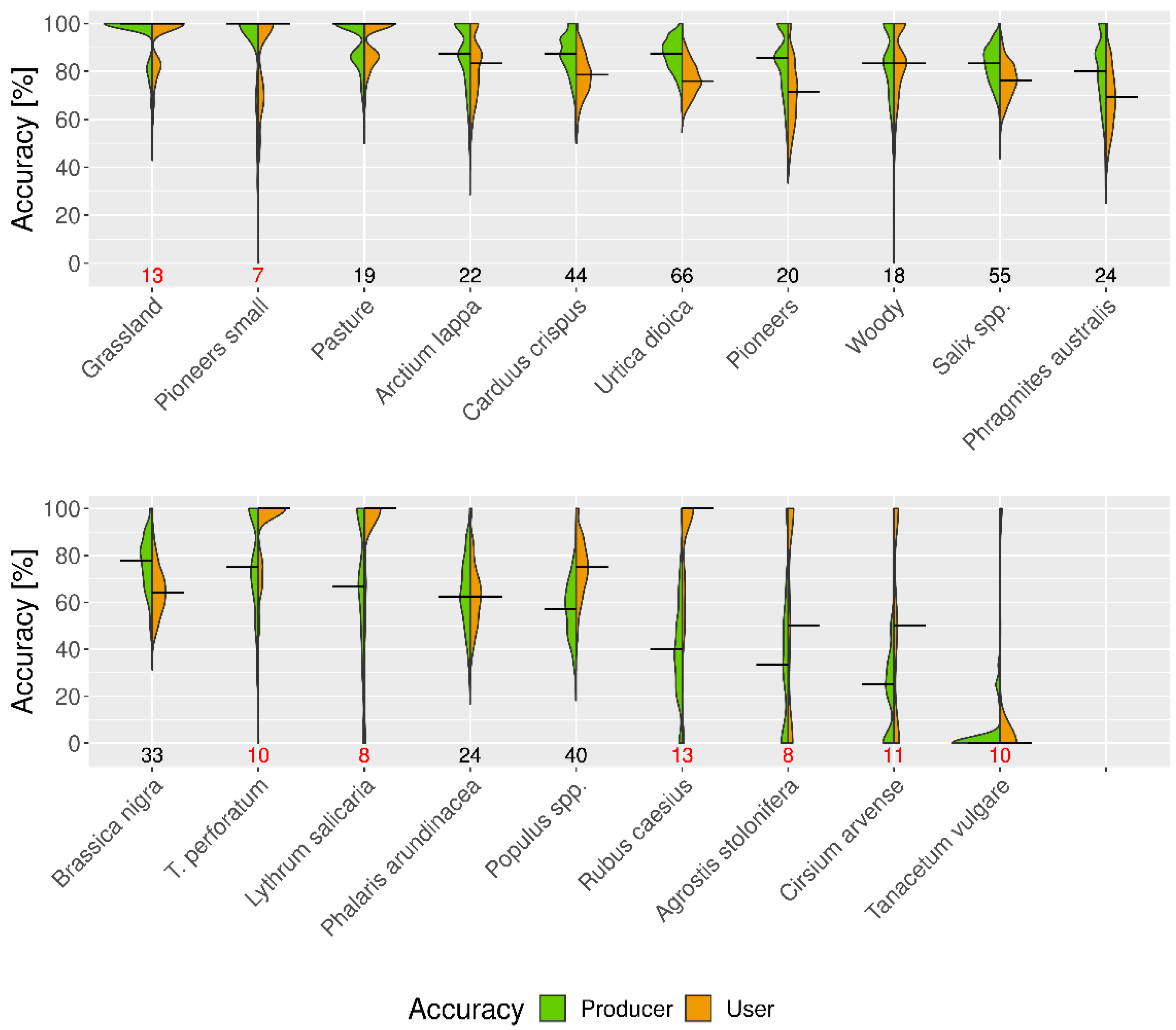
3.1.1. Results

Figure 3 displays the resulting classification maps for all thematic levels of riparian vegetation and hydromorphological substrate types using the aforementioned workflow with RF and UAS-based features. Accuracy measures using different algorithms and platforms are presented in

Table 4. Accuracy measures based on accumulated confusion matrices over 500 bootstrap iterations for each classification level, algorithm (RF = Random Forest, SVM = Support Vector Machine, XGBoost = Extreme Gradient Boost) and platform (gyrocopter, UAS = unmanned aerial system). The accuracy measures used are overall accuracy (OA), Kappa coefficient (Kc), producer’s accuracy (PA), user’s accuracy (UA) and the number of reference points for training and validation (n).

Classification Level with Classified Classes	UAS							Gyrocopter
	RF		SVM		XGBoost			RF
	PA	UA	PA	UA	PA	UA	n	PA	UA	n
Basic surface types (BA)	OA = 88.9 Kc = 0.85		OA = 88.6 Kc = 0.85		OA = 88.3 Kc = 0.85			OA = 88.4 Kc = 0.85
Water	90	88	90	87	89	88	150	87	94	156
Water shallow	77	81	75	83	77	80	165	79	85	172
Substrate types	88	93	88	92	87	93	259	87	94	244
Substrate types wet	83	76	85	77	82	76	198	90	78	232
Vegetation	96	94	95	94	96	94	623	97	90	555
Vegetation shadow	80	89	80	87	81	86	180	72	89	170
Vegetation units (VE)	OA = 88.4 Kc = 0.82		OA = 89.2 Kc = 0.83		OA = 89.1 Kc = 0.83			OA = 86.4 Kc = 0.79
Grassland	95	91	91	88	90	94	27	95	96
Herbaceous vegetation	94	92	94	92	94	92	222	93	91	221
Pioneers	84	83	83	91	85	76	40	83	89	37
Reed	72	71	76	78	71	83	48	65	65	49
Woody	83	90	85	87	87	89	81	79	81
Dominant stands (DO)	OA = 74.8 Kc = 0.72		OA = 73.8 Kc = 0.71		OA = 66.5 Kc = 0.63			OA = 65.6 Kc = 0.62
Agrostis stolonifera	32	65	37	50	8	14	8	13	28
Arctium lappa	86	80	89	84	75	77	22	76	78
Brassica nigra	76	64	82	66	64	60	33	63	55
Carduus crispus	87	77	90	79	77	71	44	81	72	47
Cirsium arvense	20	53	9	21	8	13	11	19	38
Grassland	95	92	81	69	81	81	13	78	72	15
Lythrum salicaria	68	92	62	64	99	99	8	67	97
Pasture	92	91	73	86	91	88	19	74	82	18
Phalaris arundinacea	64	62	61	49	64	65	24	54	54	25
Phragmites australis	79	67	66	61	77	66	24	61	59
Pioneers	83	70	61	82	72	63	20	84	80
Pioneers small	88	84	97	79	84	93	7	90	82	6
Populus spp.	57	73	73	79	49	55	40	59	63	39
Rubus caesius	38	79	75	82	39	46	13	40	47
Salix spp.	82	75	75	83	74	72	55	71	63	56
Tanacetum vulgare	4	19	9	18	12	16	10	1	4	11
Tripleurospermum perforatum	76	89	66	62	8	13	10	79	63
Urtica dioica	87	76	86	84	80	70	66	77	68	61
Woody	82	82	81	75	74	81	18	47	73	15
Substrate types (SU)	OA = 62 Kc = 0.53		OA = 64.9 Kc = 0.56		OA = 59.7 Kc = 0.50			OA = 52 Kc = 0.37
Armour stones	73	70	83	74	74	74	22	24	62
Fine grained material	68	58	66	61	60	57	29	66	55
Gravel	73	68	79	68	70	66	75	73	54
Sand	65	69	69	73	58	61	59	49	49
Layer of shells	64	68	56	68	67	71	18	52	60
Stones	28	50	21	44	34	42	17	5	17
Wood	33	32	36	38	34	34	29	16	29

. In this section we are focusing on the RF results of UAS data (first column).

High classification performance of RF was achieved for the level BA (OA = 88.9%) and VE (OA = 88.4%). PA and UA were ranging between 96% and 76% for BA and between 95% and 71% for VE with intra-class variation ranging from less than 7% (BA) up to 16% (VE). The classification of the level DO (OA = 74.8%) resulted in PA and UA between 95% and 4% with intra-class variation reaching up to 100% (Figure 4). Visual interpretation showed that homogeneous or larger stands were mapped correctly (e.g., Brassica nigra or Urtica dioica) For the thematic level SU an OA = 62% was achieved with class-specific accuracy measures between 73% and 28% and an intra-class variation of up to 33%. The confusion matrices for all levels and the variation in PA and UA for the levels BA, VE, and SU can be found in the Supplementary materials (Tables S1–S4 and Figures S1–S3).

Regarding feature selection for RF, 24 out of 63 potential features were selected for BA. The top five features with the highest discrimination power were only spectral indices (total brightness, GVI, gNDVI, NDWI and NDRE). Thirty features were selected for VE and 32 for DO. In these two classification levels, the features nDSM, FDM, and “different neighbor” were among the five most important ones. Among the 25 chosen features in SU classification, textural features were predominant. All selected features and importance values can be found in the Supplementary materials (Figures S6–S9).

3.1.2. Discussion

Classification performance decreased with increasing detail of the thematic level. It was high and stable for classes in the BA and VE levels, but class dependent for the DO and SU levels with high variation for classes with low sample sizes.

Results of the BA and VE level classification were comparable to other studies classifying riparian ecosystems using UAS imagery. Gómez-Sapiens et al. [19] achieved overall accuracies between 87% and 96% depending on the study site in a study focusing on vegetation cover with four vegetation and three non-vegetation classes along the Colorado river. In their study, very high accuracies were reported for water (PA/UA = 100/100% vs. 90/88% in our study) and substrate types (PA/UA = 99–100/80–100% vs. 88/93%), but low accuracies for Herbaceous vegetation (PA/UA = 58/50% vs. 94/92%). The lower accuracies in our study regarding the classes water and substrate types are mainly due to the inclusion of the similar classes water shallow and substrate types wet, which we used initially for a more detailed analysis of substrate types. Misclassification occurred mostly between classes of the same cover type, such as vegetation and vegetation shadow, substrate types and substrate types wet or water and water shallow and are therefore explainable: if for the class substrate types, misclassified samples of substrate types wet are included, the PA of substrate types would increase to 98%. The same is true for the class water/water shallow (=PA of 100%) or vegetation/vegetation shadow (=PA of 99%). Depending on the research question classes could be aggregated, which in our case would lead to an increase in classification performance. van Iersel, Straatsma, Middelkoop and Addink [18] evaluated the potential of multitemporal imagery for mapping six vegetation and four non-vegetation classes at a distributary of the Rhine river in the Netherlands. Their classification with one time-step resulted in OA of 91.6% with PA/UA of e.g., 87/96% for reed (vs. 72/71% in our study), 96/86% for pioneers (vs. 84/83%) and 74/79% for herbaceous vegetation (vs. 94/92%). Including multitemporal imagery of up to six time-steps within a year increased OA to 99.3%. Even though multitemporal imagery can increase classification performance, which is also reported in the study by Michez et al. [22], it needs to be considered that multitemporal imagery also requires more resources, such as time spent in the field and cost of data acquisition, which may be limited in practice.

Regarding DO classification, we considered PA and UA values of 60% and greater to be sufficient. This was true for 14 out of 19 classes and mainly included those forming homogeneous stands. The classes Populus spp., Rubus caesius, Cirsium arvense, Agrostis stolonifera and Tanacetum vulgare were mapped insufficiently. Tanacetum vulgare, Cirsium arvense and the small grass Agrostis stolonifera occurred mainly in small patches, growing between other species and thus leading to segments with mixed spectral signals.

Populus spp. was often confused with Salix spp. Dunford, et al. [77] also reported problems with distinguishing among the two taxa wherefore Gómez-Sapiens et al. [19] combined both classes to Cottonwood-Willow and achieved PA values of 82–97% and UA values of 75–88%. Thus, an aggregation of both classes would improve the classification.

All insufficiently classified classes, with the exception of Populus spp., had small sampling sizes of reference data (n ≤ 13) and high intra-class variation. The latter was generally observed in cases of underrepresented classes, such as Lythrum salicaria or Tripleurospermum perforatum. A small sampling size may fail to represent the population the sample was drawn from, including the spectral intra-class variation [78], and may thus have a negative influence on classification results [33,79]. In fact, we applied our workflow to another area named Nonnenwerth, also located on the river Rhine. In this case, we only distinguished between seven classes of DO, because no others were present, and achieved higher accuracies: Rubus caesius was classified with PA = 79% and UA = 85% having 29 reference points versus PA = 38% and UA = 79% resulting from the analysis of this study on Emmericher Ward using 13 reference points. The desired quantity and quality (random sampling) of reference data were not always possible, especially for higher thematic classes, which may negatively affect the explanatory power of the results [71]. Unfortunately, limitations in reference data collection are not uncommon [32] and a statistically proper sampling may even be unfeasible in most management projects due to time constraints or inaccessibility.

In order to obtain information on classes that have a low spatial coverage but are of special interest, e.g., as they are protected or typical for riparian ecosystems, we decided to include all classes in our study, even if they consist of a low sample size. One of these classes is Lythrum salicaria, a species typically occurring along the river Rhine. Within our study site, it can mainly be found at one location in a larger patch of approximately 460 m² (Figure 5). Even though PA was not very high (68% with strong variation of >40%), visual interpretation showed that this patch was mostly mapped correctly. On the other hand, UA of 92% appears too high as the correctly classified area marked in blue has too few reference points. Other examples of classes with low sample sizes, but with good classification results are pasture and grassland. Overall, good results can be achieved for classes with small sampling sizes, which was especially true for larger homogeneous stands, but higher sampling size may increase classification performance and robustness of the results.

Classification results varied for the thematic level SU as well. For instance, the class armour stones reached a PA of 73%, while stones and wood had PA values as low as 28% and 33% respectively and an intra-class variation of up to 33%. The majority of segments, located next to vegetation was wrongly classified as wood. Contrarily, van Iersel, Straatsma, Middelkoop and Addink [18] were able to differentiate between rock/rubble and bare sand with very high PA and UA from 98% and more. Compared to this study, our results for the classification accuracy were moderate. However, we differentiated between seven substrate types. An increased number of defined classes decreases classification results [24,33], which can be seen in our study regarding vegetation classification (VE with 6 classes: OA = 88.4%; DO with 19 classes: OA = 72.6%).

3.2. Comparison of Algorithms

3.2.1. Results

The classification using RF was compared with those using SVM and XGBoost. Classification with SVM and XGBoost resulted in similar OA’s for the thematic levels BA and VE as with RF where OA exhibited a less than 1% difference among algorithms (Table 4). Considering OA’s, over 500 iterations for each algorithm showed an intra-algorithm variation of 1–2% for BA and 3% for VE. Differences in OA among algorithms increased up to 5.4% for the levels DO and SU with an intra-algorithm variation of 4–5% (DO) and 5–8% (SU). PA and UA as well as visual evaluation were similar among algorithms concerning the classes of the BA and VE levels. For the levels DO and SU, results among algorithms depended on the class considered. For instance, RF outperformed SVM for the DO classes pioneers (+22% in PA with RF vs. SVM) and pasture (+19%) while the opposite was true for Rubus caesius (+37% in PA with SVM vs. RF) and Populus spp. (+16%). In most of the DO classes, PA was higher with RF than with XGBoost. DO classification with SVM resulted in more heterogeneous maps than with RF or XGBoost (Figure 6). For instance, small canopy gaps in forested areas were indeed mapped correctly with SVM as herbaceaus vegetation (level VE) but were misclassified in DO classification. RF and XGBoost labeled those canopy gaps as classes of woody vegetation, which may also not be correct, but as the surrounding areas are covered by woody vegetation this error is negligible. The same was true regarding areas of pasture (VE and DO levels) or wood and fine-grained material of SU classification (Figure 7). However, RF misclassified small poplar trees (Populus spp.) directly located on the river, whereas they were classified correctly with SVM. Visual evaluation of SU classification revealed that the results of RF and SVM show a clear distinction of substrates (referring to sand and gravel on the sand bank, Figure 7) whereby the RF classification demonstrated the most accurate mapping of the riverbank substrates. Around the riverbank, woody areas are clearly overstated by all algorithms. While the RF results show the inhomogeneous substrate distribution of the banks (shells, gravel, sand, wood), the mineral substrates are only sporadically recorded in the SVM results. Other misclassifications of substrate distribution (RF and SVM) are due to transitional areas between wet and moist substrate classes.

3.2.2. Discussion

The comparison of algorithms showed that for the BA and VE thematic levels results were similar. A more distinct separation could be seen for the levels DO and SU, however no algorithm was superior to all classes. RF was favored, as the heterogeneity in SVM classification makes a visual application in the field more difficult.

SVM has the advantage that the algorithm is insensitive to small sampling sizes as for instance reported by Burai, et al. [80]. Even though SVM had higher PA values than RF, some classes with small sampling sizes like Agrostis stolonifera or Rubus caesius demonstrated intra-class variations that were comparable to RF. Hence, the insensitivity of SVM to small sampling sizes was neither confirmed nor disconfirmed by our study. The sampling sizes of most classes of DO in this study were probably too small. A direct comparison of algorithms would require a balanced and sufficient sampling size, which remains challenging in anthropogenic modified and fragmented habitats.

Both RF and SVM revealed their strength in terms of accuracy measures and visual interpretation. A general improvement of the results may be achieved by combining both models to a single one as in the study by Xu, et al. [81] using the C5.0 algorithm. Even though model complexity increased, the computational time was still low. In fact, XGBoost took the most computation time of all models in their study, which is in line with our study, where median XGBoost computational times was up to seven times slower than RF and nine times slower than SVM.

In summary, applying SVM and XGBoost instead of RF did not increase classification performance in our study which is why we chose RF for all further analysis since accuracy measures were good, visual evaluation was convenient, computation time was low and RF was already successfully used by other studies for mapping riparian ecosystems [18,33,34].

3.3. Spatial Evaluation of Classification Probability

3.3.1. Results

To identify areas of low classification performance, we used probability maps (Figure 8) based on the results of the RF algorithm. For vegetation, two types of areas of low classification performance were identified: those located within the transition zone and shaded areas. Here, the transition zone is an area, containing a mixture of vegetation and bare ground, between dense vegetation and the waterbody (We derived the span of this zone from the mean water level to the most inland segment of bare ground plus a buffer of 9 m. Additionally, segments of vegetation that were closer to the water than the mean water level were counted too). Shaded areas were automatically identified in the BA classification (class vegetation shadow). As shown in Figure 9, classified objects of the VE level located within the transition zone had median classification probabilities of 70% while shaded objects (not counting those in the transition zone) exhibit median values of 63%. In contrast, classification was more stable in unshaded areas that were covered by dense vegetation (90%). The same pattern of classification probability appeared in the DO classification, but the values and differences between median probabilities were generally lower.

Within the transition zone, lower classification probability was also obtained for SU classification (42%) compared to areas without interference of vegetation (58%).

3.3.2. Discussion

Classification probability in our study area seems to depend on illumination and whether the classified object is located within the transition zone or not. Apart from overall probability, information can also be given for each class. For instance, Figure 5 shows lower classification probabilities for segments that were wrongly classified as Lythrum salicaria (marked in blue) and also for segments exhibiting a lower coverage of this class (on the right-hand side in Figure 5b).

A low classification probability does not necessarily mean that an area is classified wrong. However, this was often the case when the area was within a transition zone or shaded. For instance, shaded pasture near the forest line was often confused with herbaceous vegetation. Shadows can lead to a reduction, or even a total loss of spectral information [82], and thus have a negative influence on classification. Lower classification probabilities in the transition zone are mainly due to a high degree of heterogeneity leading to mixed segments. These objects contain small growing vegetation (e.g., pioneer trees of Populus spp.) and bare ground. Mixed objects with predominance of vegetation in reality, mostly represented by small pioneer trees of Populus spp., were often classified as several vegetation classes. Mixed objects with predominance of substrate types containing vegetation were in most cases labeled as the SU class wood. Taking the uncertainty into account, we recommend classifying substrate types and substrate types only (the riverbed and riverbank, respectively) separately in further works. Furthermore, adapting the scale parameter in the segmentation process [83] or applying a multi-scale approach by creating a hierarchy of several single-scale segmentations [84] may improve object delineation and thus classification results. Probability maps are an efficient and easy way to identify areas with low classification performance that should be assessed more carefully in the field.

3.4. Transfer of Classification Method from UAS to Larger Scale Gyrocopter Data

3.4.1. Results

Images acquired by gyrocopter were classified with the same workflow (RF algorithm) as for UAS data resulting in OAs of 88.4% (BA), 86.4% (VE), 65.6% (DO) and 52% (SU). Single classes of BA and VE levels were classified with similar accuracies (Table 4). The highest differences occurred for the classes vegetation shadow (PA = −9% lower with gyrocopter vs. UAS) and substrate types wet (PA = +7%) for the level BA and woody (UA = −9%) for the level VE. The majority of DO and SU classes had lower classification accuracies (often even double digits, up to −35% for woody and −49% for armour stones) using gyrocopter data in comparison to UAS data. Despite lower accuracies, the spatial distribution and coverage is similar among platforms of DO classes forming large stands, such as Urtica dioica or Brassica nigra (Figure 6a,e). Areas where classes presented patchy, e.g., Phragmites australis, or small-scale alternation between occurring classes, e.g., layer of shells and sand (Figure 7), could not be captured sufficiently.

3.4.2. Discussion

Gyrocopter classification results were comparable to those using UAS data for coarser thematic classes of the levels BA and VE as well as for classes covering larger and continuous areas of the DO and SU levels.

The insufficient detection of small-scale patches may be due to the technical properties including different camera systems (primarily the absence of the Red-Edge band, RE) and a lower spatial resolution of the gyrocopter data. Studies have shown that information of the RE spectrum can increase classification performance of vegetation [85,86]. Jorge, Vallbé and Soler [46] recommend NDRE over NDVI for the identification of possible heterogeneities in the vegetation cover. In our study, the mean and standard deviation of NDRE were always among the important variables of the feature selection of UAS variables (see Figures S6–S9 in the Supplementary materials).

The gyrocopter’s lower resolution is caused by the higher flight altitude, which again is associated with stronger interference of the atmosphere. This can lead to differences in image brightness between drone and gyrocopter images after flat-field and radiometric correction was applied. To address this problem, a field spectrometer can be used for calibration as proposed by Naethe, et al. [87]. Intercalibration is essential to match information across different platforms. Reference targets in the field serve as a known ground truth with the purpose of minimizing uncertainties with respect to camera calibration and temporal changes in incoming light. Thus, camera reflectance from drone and gyrocopter could be aligned, using a stable ground truth and radiometrically calibrated field spectrometer. This may allow a more direct comparison of reflectance properties between both platforms and also application of a pre-fitted model from one data source to another. Even though those technical properties need to be considered, we will not stress this in further detail. The focus of this study was to evaluate the use of a gyrocopter for mapping riparian waterways.

For a direct comparison among both platforms, only the area covered by UAS was used for gyrocopter classification (59 ha). Our results indicate that good class-dependent results may be achieved by classifying the whole area covered by the gyrocopter, which was approximately 1220 ha in this study, even though classification results achieved with the gyrocopter do not allow precise statements about the substrate distribution. However, with gyrocopter images, various additional hydromorphological information can be obtained for a large area. These include, for example, the condition of the riparian zone, either being natural/near-natural or consisting of constructions. From the BA, additional detailed information on the prevailing hydromorphological structure (e.g., shallow water zones, pools, island areas) can be derived. Depending on the research question and management aim, UAS should be used when small-scale patches of vegetation and substrate types need to be monitored. Furthermore, we used UAS imagery as a valuable source for reference data collection [88].

Taking practical consideration into account, the data collection for each platform took approximately one day for the respective areas with an additional day in the field for GCP collection (the same GCPs were used for both platforms). Covering larger areas solely with UAS can quickly exceed cost budgets [18]. Hence, we recommend using a gyrocopter for surveys of larger areas (>1 km²) and UAS for smaller areas (<1 km²). Ideally, whenever larger areas are surveyed by gyrocopter, smaller areas of interest and for reference data collection are recorded by UAS, while intercalibrating all camera systems.

4. Conclusions

In this study, we proposed an object-based image analysis workflow to classify vegetation and substrate types with different level of detail, using multispectral very high-resolution UAS and gyrocopter imagery in a riparian ecosystem along the river Rhine in Germany. With reference to the numbering of the four research questions, our conclusions are:

(I)

Classification results for UAS data with RF decreased with increasing class detail from BA (OA = 88.9%) and VE (OA = 88.4%) to DO (OA = 74.8%) and SU (OA = 62%). Classes with high spatial coverage or those which are homogeneous could be mapped sufficiently. Classes with low sample sizes had high intra-class variability and, even when good median accuracies were achieved. In general, RF was a suitable algorithm to classify vegetation and substrate types in riparian zones. The results of the feature selections showed for BA level, that the spectral indices have the largest explanatory power in the models, whereas for the VE and DO level the highest explanatory power lies on the hydrotopographic parameters and for the SU level textural indices were predominant.

(II)

Classification performance did not change notably when using SVM or XGBoost instead of RF. SVM introduced more heterogeneous and patchy maps while classifying vegetation that did not match with the visual interpretation and would be difficult to work with in the field. On the other hand, XGBoost consumed the highest computational time. Thus, for the rest of this study RF was used.

(III)

Classification probability maps can be used to identify areas of low performance and prioritize them during (re-)visits in the field. For instance, areas located in the transition zone and shaded areas of vegetation had low classification probabilities and were often classified incorrectly. Hence, when using probability maps efficiency of field surveys may be increased.

(IV)

Gyrocopter data can be used within the same classification workflow and achieve comparable results as UAS data for classes of the levels BA and VE as well as for classes covering larger and homogeneous areas. For management purposes, it might be useful to collect information over larger areas, possibly in combination with UAS.

Overall, this study demonstrated that UAS and gyrocopter data can be used in combination with machine learning techniques to retrieve information about vegetation and substrate types distribution in riparian zones, which may be used for management actions such as monitoring and assessing of measures to improve ecological status.

5. Outlook and Further Work

Possibilities for further research and development of the approach are:

• To apply the workflow on the whole gyrocopter area and including classes, such as “urban areas” or “agriculture”, which are not represented in the area under investigation in this study. This step also includes the collection of training and validation data of those classes based on the imagery.
• To evaluate the transferability of the classification workflow in new areas. This step also includes the application of the already existing classification models on new areas and evaluation of the question of what extent the existing reference data can be used in addition to newly collected reference data to build new models.
• To examine the effect of multi-temporal imagery on classification results, as demonstrated by van Iersel, Straatsma, Middelkoop and Addink [18], and to evaluate if a potential increase in classification performance may justify the additional workload.
• To implement the proposed workflow in management routines of the waterway and shipping administration and to adjust them to the future needs of the stakeholder concerns [13]. Potential routine could be to use the classification maps as a basis for more detailed vegetation mapping or to use them within the hydromorphological evaluation and classification tool, Valmorph [89].

References

1. Baattrup-Pedersen, A.; Jensen, K.M.B.; Thodsen, H.; Andersen, H.E.; Andersen, P.M.; Larsen, S.E.; Riis, T.; Andersen, D.K.; Audet, J.; Kronvang, B. Effects of stream flooding on the distribution and diversity of groundwater-dependent vegetation in riparian areas. Freshw. Biol. 2013, 58, 817–827. [Google Scholar] [CrossRef]
2. Capon, S.J.; Pettit, N.E. Turquoise is the new green: Restoring and enhancing riparian function in the Anthropocene. Ecol. Manag. Restor. 2018, 19, 44–53. [Google Scholar] [CrossRef]
3. Chakraborty, S.K. Riverine Ecology; Springer International Publishing: Basel, Switzerland, 2021; Volume 2, ISBN 978-3-030-53941-2. [Google Scholar]
4. Grizzetti, B.; Liquete, C.; Pistocchi, A.; Vigiak, O.; Zulian, G.; Bouraoui, F.; De Roo, A.; Cardoso, A.C. Relationship between ecological condition and ecosystem services in European rivers, lakes and coastal waters. Sci. Total Environ. 2019, 671, 452–465. [Google Scholar] [CrossRef] [PubMed]
5. Cole, L.J.; Stockan, J.; Helliwell, R. Managing riparian buffer strips to optimise ecosystem services: A review. Agric. Ecosyst. Environ. 2020, 296, 106891. [Google Scholar] [CrossRef]
6. Meybeck, M. Global analysis of river systems: From Earth system controls to Anthropocene syndromes. Philos. Trans. R. Soc. B Biol. Sci. 2003, 358, 1935–1955. [Google Scholar] [CrossRef] [PubMed]
7. Voulvoulis, N.; Arpon, K.D.; Giakoumis, T. The EU Water Framework Directive: From great expectations to problems with implementation. Sci. Total Environ. 2017, 575, 358–366. [Google Scholar] [CrossRef] [Green Version]
8. Council of the European Commission, Council Directive 92/43/EEC of 21 May 1992 on the conservation of natural habitats and of wild fauna and flora. Off. J. 1992, 206, 7–50. Available online: https://eur-lex.europa.eu/legal-content/EN/TXT/?uri=CELEX%3A31992L0043 (accessed on 12 January 2022).
9. The European Parliament and Council of the European Union, Directive 2000/60/EC of the European Parliament and of the Council Establishing a Framework for the Community Action in the Field of Water Policy. Off. J. 2020, 327, 1–73. Available online: https://eur-lex.europa.eu/legal-content/en/TXT/?uri=CELEX:32000L0060 (accessed on 12 January 2022).
10. Germany’s Blue Belt’ Programme. Available online: https://www.bundesregierung.de/breg-en/federal-government/-germany-s-blue-belt-programme-394228 (accessed on 12 January 2022).
11. Dronova, I. Object-Based Image Analysis in Wetland Research: A Review. Remote Sens. 2015, 7, 6380–6413. [Google Scholar] [CrossRef] [Green Version]
12. Ren, L.; Liu, Y.; Zhang, S.; Cheng, L.; Guo, Y.; Ding, A. Vegetation Properties in Human-Impacted Riparian Zones Based on Unmanned Aerial Vehicle (UAV) Imagery: An Analysis of River Reaches in the Yongding River Basin. Forests 2020, 12, 22. [Google Scholar] [CrossRef]
13. Huylenbroeck, L.; Laslier, M.; Dufour, S.; Georges, B.; Lejeune, P.; Michez, A. Using remote sensing to characterize riparian vegetation: A review of available tools and perspectives for managers. J. Environ. Manag. 2020, 267, 110652. [Google Scholar] [CrossRef] [PubMed]
14. Piégay, H.; Arnaud, F.; Belletti, B.; Bertrand, M.; Bizzi, S.; Carbonneau, P.; Dufour, S.; Liébault, F.; Ruiz-Villanueva, V.; Slater, L. Remotely sensed rivers in the Anthropocene: State of the art and prospects. Earth Surf. Process. Landf. 2020, 45, 157–188. [Google Scholar] [CrossRef]
15. Tomsett, C.; Leyland, J. Remote sensing of river corridors: A review of current trends and future directions. River Res. Appl. 2019, 35, 779–803. [Google Scholar] [CrossRef]
16. Langhammer, J. UAV Monitoring of Stream Restorations. Hydrology 2019, 6, 29. [Google Scholar] [CrossRef] [Green Version]
17. Arif, M.S.M.; Gülch, E.; Tuhtan, J.A.; Thumser, P.; Haas, C. An investigation of image processing techniques for substrate classification based on dominant grain size using RGB images from UAV. Int. J. Remote Sens. 2016, 38, 2639–2661. [Google Scholar] [CrossRef]
18. Van Iersel, W.; Straatsma, M.; Middelkoop, H.; Addink, E. Multitemporal Classification of River Floodplain Vegetation Using Time Series of UAV Images. Remote Sens. 2018, 10, 1144. [Google Scholar] [CrossRef] [Green Version]
19. Gómez-Sapiens, M.; Schlatter, K.J.; Meléndez, Á.; Hernández-López, D.; Salazar, H.; Kendy, E.; Flessa, K.W. Improving the efficiency and accuracy of evaluating aridland riparian habitat restoration using unmanned aerial vehicles. Remote Sens. Ecol. Conserv. 2021, 7, 488–503. [Google Scholar] [CrossRef]
20. van Iersel, W.; Straatsma, M.; Addink, E.; Middelkoop, H. Monitoring height and greenness of non-woody floodplain vegetation with UAV time series. ISPRS J. Photogramm. Remote Sens. 2018, 141, 112–123. [Google Scholar] [CrossRef]
21. Martin, F.-M.; Müllerová, J.; Borgniet, L.; Dommanget, F.; Breton, V.; Evette, A. Using Single- and Multi-Date UAV and Satellite Imagery to Accurately Monitor Invasive Knotweed Species. Remote Sens. 2018, 10, 1662. [Google Scholar] [CrossRef] [Green Version]
22. Michez, A.; Piégay, H.; Jonathan, L.; Claessens, H.; Lejeune, P. Mapping of riparian invasive species with supervised classification of Unmanned Aerial System (UAS) imagery. Int. J. Appl. Earth Obs. Geoinf. 2016, 44, 88–94. [Google Scholar] [CrossRef]
23. IKSR. Überblicksbericht über die Entwicklung des ‘Biotopverbund am Rhein’ 2005–2013; Internationale Kommission zum Schutz des Rheins: Koblenz, Germany, 2015; ISBN 3-941994-79-4. [Google Scholar]
24. Ma, L.; Li, M.; Ma, X.; Cheng, L.; Du, P.; Liu, Y. A review of supervised object-based land-cover image classification. ISPRS J. Photogramm. Remote Sens. 2017, 130, 277–293. [Google Scholar] [CrossRef]
25. Weber, I.; Jenal, A.; Kneer, C.; Bongartz, J. Gyrocopter-based remote sensing platform. ISPRS Int. Arch. Photogramm. Remote Sens. Spat. Inf. Sci. 2015, XL-7/W3, 1333–1337. [Google Scholar] [CrossRef] [Green Version]
26. Fricke, K.; Baschek, B.; Jenal, A.; Kneer, C.; Weber, I.; Bongartz, J.; Wyrwa, J.; Schöl, A. Observing Water Surface Temperature from Two Different Airborne Platforms over Temporarily Flooded Wadden Areas at the Elbe Estuary—Methods for Corrections and Analysis. Remote Sens. 2021, 13, 1489. [Google Scholar] [CrossRef]
27. Calvino-Cancela, M.; Mendez-Rial, R.; Reguera-Salgado, J.; Martin-Herrero, J. Alien Plant Monitoring with Ultralight Airborne Imaging Spectroscopy. PLoS ONE 2014, 9, e102381. [Google Scholar] [CrossRef] [PubMed]
28. Hellwig, F.M.; Stelmaszczuk-Górska, M.A.; Dubois, C.; Wolsza, M.; Truckenbrodt, S.C.; Sagichewski, H.; Chmara, S.; Bannehr, L.; Lausch, A.; Schmullius, C. Mapping European Spruce Bark Beetle Infestation at Its Early Phase Using Gyrocopter-Mounted Hyperspectral Data and Field Measurements. Remote Sens. 2021, 13, 4659. [Google Scholar] [CrossRef]
29. Manfreda, S.; McCabe, M.F.; Miller, P.E.; Lucas, R.; Madrigal, V.P.; Mallinis, G.; Ben Dor, E.; Helman, D.; Estes, L.; Ciraolo, G.; et al. On the Use of Unmanned Aerial Systems for Environmental Monitoring. Remote Sens. 2018, 10, 641. [Google Scholar] [CrossRef] [Green Version]
30. Jiménez López, J.; Mulero-Pázmány, M. Drones for Conservation in Protected Areas: Present and Future. Drones 2019, 3, 10. [Google Scholar] [CrossRef] [Green Version]
31. Mahdavi, S.; Salehi, B.; Granger, J.; Amani, M.; Brisco, B.; Huang, W. Remote sensing for wetland classification: A comprehensive review. GISci. Remote Sens. 2017, 55, 623–658. [Google Scholar] [CrossRef]
32. Maxwell, A.E.; Warner, T.A.; Fang, F. Implementation of machine-learning classification in remote sensing: An applied review. Int. J. Remote Sens. 2018, 39, 2784–2817. [Google Scholar] [CrossRef] [Green Version]
33. Zhang, C.; Xie, Z. Object-based Vegetation Mapping in the Kissimmee River Watershed Using HyMap Data and Machine Learning Techniques. Wetlands 2013, 33, 233–244. [Google Scholar] [CrossRef]
34. Nguyen, U.; Glenn, E.P.; Dang, T.D.; Pham, L. Mapping vegetation types in semi-arid riparian regions using random forest and object-based image approach: A case study of the Colorado River Ecosystem, Grand Canyon, Arizona. Ecol. Inform. 2019, 50, 43–50. [Google Scholar] [CrossRef]
35. Fassnacht, F.E.; Latifi, H.; Stereńczak, K.; Modzelewska, A.; Lefsky, M.; Waser, L.T.; Straub, C.; Ghosh, A. Review of studies on tree species classification from remotely sensed data. Remote Sens. Environ. 2016, 186, 64–87. [Google Scholar] [CrossRef]
36. Georganos, S.; Grippa, T.; VanHuysse, S.; Lennert, M.; Shimoni, M.; Kalogirou, S.; Wolff, E. Less is more: Optimizing classification performance through feature selection in a very-high-resolution remote sensing object-based urban application. GIScience Remote Sens. 2017, 55, 221–242. [Google Scholar] [CrossRef]
37. Sandino, J.; Gonzalez, F.; Mengersen, K.; Gaston, K.J. UAVs and Machine Learning Revolutionising Invasive Grass and Vegetation Surveys in Remote Arid Lands. Sensors 2018, 18, 605. [Google Scholar] [CrossRef] [PubMed] [Green Version]
38. Zhang, H.; Eziz, A.; Xiao, J.; Tao, S.; Wang, S.; Tang, Z.; Zhu, J.; Fang, J. High-Resolution Vegetation Mapping Using eXtreme Gradient Boosting Based on Extensive Features. Remote Sens. 2019, 11, 1505. [Google Scholar] [CrossRef] [Green Version]
39. Congalton, R.G.; Green, K. Assessing the Accuracy of Remotely Sensed Data: Principles and Practices, 3rd ed.; CRC Press: Boca Raton, FL, USA, 2019; ISBN 0429629354. [Google Scholar]
40. Malley, J.D.; Kruppa, J.; Dasgupta, A.; Malley, K.G.; Ziegler, A. Probability Machines. Methods Inf. Med. 2012, 51, 74–81. [Google Scholar] [CrossRef]
41. Millard, K.; Richardson, M. On the Importance of Training Data Sample Selection in Random Forest Image Classification: A Case Study in Peatland Ecosystem Mapping. Remote Sens. 2015, 7, 8489–8515. [Google Scholar] [CrossRef] [Green Version]
42. UNEP-WCMC. Protected Area Profile for Nsg Emmericher Ward from the World Database of Protected Areas. Available online: www.protectedplanet.net (accessed on 20 December 2021).
43. Westoby, M.J.; Brasington, J.; Glasser, N.F.; Hambrey, M.J.; Reynolds, J.M. ‘Structure-from-Motion’ photogrammetry: A low-cost, effective tool for geoscience applications. Geomorphology 2012, 179, 300–314. [Google Scholar] [CrossRef] [Green Version]
44. Jensen, J.R. Remote Sensing of the Environment: An Earth Resource Perspective; Pearson Prentice Hall: Upper Saddle River, NJ, USA, 2007; ISBN 9780136129134. [Google Scholar]
45. Xue, J.; Su, B. Significant Remote Sensing Vegetation Indices: A Review of Developments and Applications. J. Sens. 2017, 2017, 1353691. [Google Scholar] [CrossRef] [Green Version]
46. Jorge, J.; Vallbé, M.; Soler, J.A. Detection of irrigation inhomogeneities in an olive grove using the NDRE vegetation index obtained from UAV images. Eur. J. Remote Sens. 2019, 52, 169–177. [Google Scholar] [CrossRef] [Green Version]
47. Michez, A.; Piégay, H.; Lisein, J.; Claessens, H.; Lejeune, P. Classification of riparian forest species and health condition using multi-temporal and hyperspatial imagery from unmanned aerial system. Environ. Monit. Assess. 2016, 188, 146. [Google Scholar] [CrossRef] [PubMed] [Green Version]
48. Mishra, V.N.; Prasad, R.; Rai, P.K.; Vishwakarma, A.K.; Arora, A. Performance evaluation of textural features in improving land use/land cover classification accuracy of heterogeneous landscape using multi-sensor remote sensing data. Earth Sci. Inform. 2018, 12, 71–86. [Google Scholar] [CrossRef]
49. Laliberte, A.S.; Rango, A. Texture and Scale in Object-Based Analysis of Subdecimeter Resolution Unmanned Aerial Vehicle (UAV) Imagery. IEEE Trans. Geosci. Remote Sens. 2009, 47, 761–770. [Google Scholar] [CrossRef] [Green Version]
50. Haralick, R.M.; Shanmugam, K.; Dinstein, I.H. Textural Features for Image Classification. IEEE Trans. Syst. Man Cybern. 1973, SMC-3, 610–621. [Google Scholar] [CrossRef] [Green Version]
51. Gini, R.; Sona, G.; Ronchetti, G.; Passoni, D.; Pinto, L. Improving Tree Species Classification Using UAS Multispectral Images and Texture Measures. ISPRS Int. J. Geo-Inf. 2018, 7, 315. [Google Scholar] [CrossRef] [Green Version]
52. Dorigo, W.; Lucieer, A.; Podobnikar, T.; Čarni, A. Mapping invasive Fallopia japonica by combined spectral, spatial, and temporal analysis of digital orthophotos. Int. J. Appl. Earth Obs. Geoinf. 2012, 19, 185–195. [Google Scholar] [CrossRef]
53. Trimble. eCognition Developer 10.1 Reference Book; Trimble Germany GmbH: Munich, Germany, 2021. [Google Scholar]
54. Tu, Y.-H.; Johansen, K.; Phinn, S.; Robson, A. Measuring Canopy Structure and Condition Using Multi-Spectral UAS Imagery in a Horticultural Environment. Remote Sens. 2019, 11, 269. [Google Scholar] [CrossRef] [Green Version]
55. Kupidura, P.; Osińska-Skotak, K.; Lesisz, K.; Podkowa, A. The Efficacy Analysis of Determining the Wooded and Shrubbed Area Based on Archival Aerial Imagery Using Texture Analysis. ISPRS Int. J. Geo-Inf. 2019, 8, 450. [Google Scholar] [CrossRef] [Green Version]
56. Weber, A. Annual flood durations along River Elbe and Rhine from 1960–2019 computed with flood3. in preparation.
57. Benz, U.C.; Hofmann, P.; Willhauck, G.; Lingenfelder, I.; Heynen, M. Multi-resolution, object-oriented fuzzy analysis of remote sensing data for GIS-ready information. ISPRS J. Photogramm. Remote Sens. 2004, 58, 239–258. [Google Scholar] [CrossRef]
58. R Core Team. R: A Language and Environment for Statistical Computing; R Foundation for Statistical Computing: Vienna, Austria, 2021. [Google Scholar]
59. Guyon, I.; Elisseeff, A. Introduction to Variable and Feature Selection. J. Mach. Learn. Res. 2003, 3, 1157–1182. [Google Scholar]
60. Bommert, A.; Sun, X.; Bischl, B.; Rahnenführer, J.; Lang, M. Benchmark for filter methods for feature selection in high-dimensional classification data. Comput. Stat. Data Anal. 2020, 143, 106839. [Google Scholar] [CrossRef]
61. Wright, M.N.; Ziegler, A. Ranger: A fast implementation of random forests for high dimensional data in C++ and R. J. Stat. Softw. 2017, 77, 1–17. [Google Scholar] [CrossRef] [Green Version]
62. Belgiu, M.; Drăguţ, L. Random forest in remote sensing: A review of applications and future directions. ISPRS J. Photogramm. Remote Sens. 2016, 114, 24–31. [Google Scholar] [CrossRef]
63. Breiman, L. Random forests. Mach. Learn. 2001, 45, 5–32. [Google Scholar] [CrossRef] [Green Version]
64. Cortes, C.; Vapnik, V. Support-vector networks. Mach. Learn. 1995, 20, 273–297. [Google Scholar] [CrossRef]
65. Mountrakis, G.; Im, J.; Ogole, C. Support vector machines in remote sensing: A review. ISPRS J. Photogramm. Remote Sens. 2011, 66, 247–259. [Google Scholar] [CrossRef]
66. Chen, T.; Guestrin, C. XGBoost. In Proceedings of the 22nd ACM SIGKDD International Conference on Knowledge Discovery and Data Mining, San Francisco, CA, USA, 13–17 August 2016; pp. 785–794. [Google Scholar]
67. Bischl, B.; Lang, M.; Kotthoff, L.; Schiffner, J.; Richter, J.; Studerus, E.; Casalicchio, G.; Jones, Z. mlr: Machine Learning in R. J. Mach. Learn. Res. 2016, 17, 5938–5942. [Google Scholar]
68. Meyer, D.; Dimitriadou, E.; Hornik, K.; Weingessel, A.; Leisch, F.; Chang, C.-C.; Lin, C.-C. e1071: Misc Functions of the Department of Statistics, Probability Theory Group (Formerly: E1071), TU Wien; R Package Version 1.7-9. 2021. Available online: https://cran.r-project.org/web/packages/e1071/index.html (accessed on 12 January 2022).
69. Chen, T.; He, T.; Benesty, M.; Khotilovich, V.; Tang, Y.; Cho, H.; Chen, K.; Mitchell, R.; Cano, I.; Zhou, T.; et al. xgboost: Extreme Gradient Boosting; R Package Version 1.5.0.1; 2021. Available online: https://cran.r-project.org/web/packages/xgboost/index.html (accessed on 12 January 2022).
70. Pontius, R.G., Jr.; Millones, M. Death to Kappa: Birth of quantity disagreement and allocation disagreement for accuracy assessment. Int. J. Remote Sens. 2011, 32, 4407–4429. [Google Scholar] [CrossRef]
71. Olofsson, P.; Foody, G.M.; Herold, M.; Stehman, S.V.; Woodcock, C.E.; Wulder, M.A. Good practices for estimating area and assessing accuracy of land change. Remote Sens. Environ. 2014, 148, 42–57. [Google Scholar] [CrossRef]
72. Hsiao, L.-H.; Cheng, K.-S. Assessing Uncertainty in LULC Classification Accuracy by Using Bootstrap Resampling. Remote Sens. 2016, 8, 705. [Google Scholar] [CrossRef] [Green Version]
73. Efron, B.; Tibshirani, R. An Introduction to the Bootstrap; Chapman & Hall: New York, NY, USA, 1993; ISBN 0412042312. [Google Scholar]
74. Lyons, M.B.; Keith, D.A.; Phinn, S.R.; Mason, T.J.; Elith, J. A comparison of resampling methods for remote sensing classification and accuracy assessment. Remote Sens. Environ. 2018, 208, 145–153. [Google Scholar] [CrossRef]
75. Roberts, D.R.; Bahn, V.; Ciuti, S.; Boyce, M.; Elith, J.; Guillera-Arroita, G.; Hauenstein, S.; Lahoz-Monfort, J.J.; Schroder, B.; Thuiller, W.; et al. Cross-validation strategies for data with temporal, spatial, hierarchical, or phylogenetic structure. Ecography 2017, 40, 913–929. [Google Scholar] [CrossRef]
76. Lopatin, J.; Dolos, K.; Kattenborn, T.; Fassnacht, F. How canopy shadow affects invasive plant species classification in high spatial resolution remote sensing. Remote Sens. Ecol. Conserv. 2019, 5, 302–317. [Google Scholar] [CrossRef]
77. Dunford, R.; Michel, K.; Gagnage, M.; Piégay, H.; Trémelo, M.-L. Potential and constraints of Unmanned Aerial Vehicle technology for the characterization of Mediterranean riparian forest. Int. J. Remote Sens. 2009, 30, 4915–4935. [Google Scholar] [CrossRef]
78. Hay, A.M. Sampling designs to test land-use map accuracy. Photogramm. Eng. Remote Sens. 1979, 45, 529–533. [Google Scholar]
79. Rogan, J.; Franklin, J.; Stow, D.; Miller, J.; Woodcock, C.; Roberts, D. Mapping land-cover modifications over large areas: A comparison of machine learning algorithms. Remote Sens. Environ. 2008, 112, 2272–2283. [Google Scholar] [CrossRef]
80. Burai, P.; Deák, B.; Valkó, O.; Tomor, T. Classification of Herbaceous Vegetation Using Airborne Hyperspectral Imagery. Remote Sens. 2015, 7, 2046–2066. [Google Scholar] [CrossRef] [Green Version]
81. Xu, S.; Zhao, Q.; Yin, K.; Zhang, F.; Liu, D.; Yang, G. Combining random forest and support vector machines for object-based rural-land-cover classification using high spatial resolution imagery. J. Appl. Remote Sens. 2019, 13, 014521. [Google Scholar] [CrossRef]
82. Zhang, L.; Sun, X.; Wu, T.; Zhang, H. An Analysis of Shadow Effects on Spectral Vegetation Indexes Using a Ground-Based Imaging Spectrometer. IEEE Geosci. Remote Sens. Lett. 2015, 12, 2188–2192. [Google Scholar] [CrossRef]
83. Pande-Chhetri, R.; Abd-Elrahman, A.; Liu, T.; Morton, J.; Wilhelm, V.L. Object-based classification of wetland vegetation using very high-resolution unmanned air system imagery. Eur. J. Remote Sens. 2017, 50, 564–576. [Google Scholar] [CrossRef] [Green Version]
84. Johnson, B.; Xie, Z. Unsupervised image segmentation evaluation and refinement using a multi-scale approach. ISPRS J. Photogramm. Remote Sens. 2011, 66, 473–483. [Google Scholar] [CrossRef]
85. Schuster, C.; Forster, M.; Kleinschmit, B. Testing the red edge channel for improving land-use classifications based on high-resolution multi-spectral satellite data. Int. J. Remote Sens. 2012, 33, 5583–5599. [Google Scholar] [CrossRef]
86. Li, X.; Chen, G.; Liu, J.; Cheng, X.; Liao, Y. Effects of RapidEye imagery’s red-edge band and vegetation indices on land cover classification in an arid region. Chin. Geogr. Sci. 2017, 27, 827–835. [Google Scholar] [CrossRef]
87. Naethe, P.; Asgari, M.; Kneer, C.; Knieps, M.; Jenal, A.; Weber, I.; Moelter, T.; Dzunic, F.; Deffert, P.; Rommel, E.; et al. Calibration and Validation of two levels of airborne, multi-spectral imaging using timesynchronous spectroscopy on the ground. in preparation.
88. Räsänen, A.; Virtanen, T. Data and resolution requirements in mapping vegetation in spatially heterogeneous landscapes. Remote Sens. Environ. 2019, 230, 111207. [Google Scholar] [CrossRef]
89. Quick, I.; König, F.; Baulig, Y.; Borgsmüller, C.; Schriever, S. The Hydromorphological Classification Tool Valmorph 2 for Large and Navigable Surface Waters; BfG Rep. No. 1910; Federal Institute of Hydrology: Koblenz, Germany, 2017. [Google Scholar]
Figure 1. Study area Emmericher Ward. RGB-imagery acquired by unmanned aerial system (UAS, 59 ha) and gyrocopter (1220 ha) on 23 July 2019.
Remotesensing 14 00954 g001
Figure 2. Overview of the classification workflow for classifying multispectral very-high resolution imagery acquired by unmanned aerial system (UAS) and gyrocopter in combination with additional abiotic and reference data. The classification was applied four times with different reference data to classify the levels: Basic surface types (BA), Vegetation units (VE), Dominant stands (DO) and Substrate types (SU). A digital elevation model was processed from the multispectral imagery and normalized with a digital elevation model (DEM) to a normalized digital surface model (nDSM). Algorithms used for classification were Random Forest (RF), Support Vector Machine (SVM) and Extreme Gradient Boost (XGBoost).
Remotesensing 14 00954 g002
Figure 3. Classification maps of the study area Emmericher Ward of four thematic levels based on the Random Forest algorithm and UAS data. Classes of the thematic level Basic surface type (overall accuracy, OA = 88.9%) are further broken down into Vegetation units (OA = 88.4%) and Substrate types (OA = 62%). Classes of Vegetation unit are classified in more detail on the thematic level Dominant stands (OA = 74.8%).
Remotesensing 14 00954 g003
Figure 4. Violin plots (density distribution) of intra-class variation of producer’s and user’s accuracy of dominant stand classes over 500 bootstrap iterations based on UAS data and Random Forest. Sorted by producer’s accuracy in decreasing order. Median values over 500 iterations are represented by horizontal lines (e.g., median producer’s accuracy of Grassland = 100%). Numbers of reference data are presented on x-axis; red color indicates n ≤ 13.
Remotesensing 14 00954 g004
Figure 5. Occurrence of Lythrum salicaria: (a) Comparison between occurrence in the field and classified segments plotted into RGB imagery, (b) classification probability, (c) field photo of flowering Lythrum salicaria from 23 July 2019. The subset of the map contains 97% of the area where Lythrum salicaria was classified.
Remotesensing 14 00954 g005
Figure 6. Subset of Dominant stand classification using different algorithms and features; (a) RGB unmanned aerial system (UAS) imagery; (b) classification with gyrocopter features and Random Forest (RF); (c) classification with UAS features and Random Forest, (d) and Support Vector Machine (SVM), (e) and Extreme Gradient Boost (XGBoost); see Table 4 for the complete genus names.
Remotesensing 14 00954 g006
Figure 7. Subset of Substrate types of classification using different algorithms and features; (a) RGB unmanned aerial system (UAS) imagery; (b) classification with gyrocopter features and Random Forest (RF); (c) classification with UAS features and Random Forest, (d) and Support Vector Machine (SVM), (e) and Extreme Gradient Boost (XGBoost).
Remotesensing 14 00954 g007
Figure 8. Classification probability, (a) RGB unmanned aerial system imagery with transition zone and areas of shaded vegetation; (b) subset of classification probability for the level Dominant stands and (c) Substrate types; (d) example of segmentation with mixed objects containing vegetation and substrate types.
Remotesensing 14 00954 g008
Figure 9. Violin (density distribution) and box-and-whisker plots of classification probability for each segment, grouped in several areas. Classification probability for Vegetation units and Dominant stands is lower in transition zones (n = 27,238 objects) and in shaded areas (n = 17,500 objects) than in dense and properly lit vegetation (n = 81,638 objects). Classification probability for Substrate types is lower in transition zones (n = 4539 objects) than where Substrate types occur without any vegetation (n = 10,030 objects). Classification is calculated using Random Forest and UAS data.
Remotesensing 14 00954 g009