Wide-Area Grid-Based Slant Ionospheric Delay Corrections for Precise Point Positioning

Abstract

Introducing ionospheric information into a precise point positioning (PPP) solution enables faster ambiguity resolution and significantly improves positioning accuracy. To compute such corrections over wide areas, sparse networks with potentially irregular station distributions are often used. This aspect brings a new level of complexity as ionospheric corrections should be weighted appropriately in the PPP filter. This paper presents a possible implementation of grid-based wide-area slant ionospheric delay corrections, with a focus on the reported uncertainties. A balance is obtained between obtaining corrections with formal errors small enough to enable fast convergence, while large enough to overbound most errors. Based on least-squares collocation, the method uses satellite-specific variograms based on the 99th percentile values in each distance bin. Tested in southern Canada over a 53-week period in 2020, ionospheric grids allowed dual-frequency receivers to obtain around 5 cm accuracy in each horizontal component within 5 min of static data collection. For single-frequency solutions using data from geodetic receivers, positioning errors were reduced by over 60% for both static and kinematic processing.

1. Introduction

Dual- (or multi-) frequency global navigation satellite system (GNSS) receivers can precisely measure ionospheric delays due to the dispersive properties of the medium for radio waves. Despite this characteristic, the ionosphere remains a limitation for the rapid convergence of precise point positioning (PPP) solutions [1]. Fortunately, constraining slant ionospheric delay parameters in a PPP filter using external information can enable fast, even instantaneous, cm-level positioning [2,3].

With the emergence of PPP-RTK (real-time kinematic) techniques, the state-space approach to error modeling has shown to be a flexible approach to GNSS augmentation [4]. In terms of ionospheric corrections, global ionospheric maps (GIMs) are widely used for wide-area positioning. Most GIMs use a single-layer implementation, which assumes that all electrons are contained within a thin shell at a fixed altitude. This assumption neglects the possible asymmetry in electron density and uses an approximate mapping function to convert slant to vertical total electron content (TEC). Extensive testing has shown that GIMs can typically correct around 80% of the delay, leaving residual errors of several TEC units (1 TECU ≈ 16 cm of delay on the GPS L1 signal) [5,6].

Under quiet ionospheric conditions, GIMs can considerably reduce positioning errors during the first few epochs of a session [7,8]. However, according to [9], even ionospheric corrections provided with a formal precision of 16 cm (1 TECU) have little impact on the time to resolve carrier-phase ambiguities in a PPP filter; significant benefits in terms of ambiguity resolution occur for uncertainties below 5 cm. For this reason, it is preferable to model slant ionospheric delays on a satellite-by-satellite basis. This satellite-specific approach to error modeling has long been recognized as a key component of differential positioning techniques such as network RTK (NRTK) [10].

Extending the concepts of NRTK ionospheric modeling to wider areas brings new challenges. One-way communication, required for state-space corrections, often leads to a loss of information when broadcasting corrections to users as it is not possible to transmit all information available from the network solution (e.g., correlations). Public reference networks were often not designed with the goal of providing ionospheric corrections to users and suffer from irregular station distribution. Larger inter-station distances, possibly exceeding a few hundred kilometers in some regions, necessitate that ionospheric corrections be weighted in the positioning filter rather than being considered as known quantities. These aspects bring a whole new level of complexity to the system since inadequate formal errors can have detrimental effects on rover positions.

One can turn to the Wide Area Augmentation System (WAAS) in the continental US for lessons learned on uncertainty characterization. The use of Kriging has proven to be a useful tool in increasing the accuracy [11] and availability [12] of the system. Variograms depict the variability of the ionosphere and can be tuned to overbound observed disturbances [13]. This concept is of particular interest in our study as it is preferable to provide slightly larger uncertainties to users to avoid over-constraining parameters in the PPP filter. While the WAAS implementation further inflates uncertainties to maintain a high level of integrity, this approach is not necessary for non-safety-critical applications. Other notable distinctions between the proposed PPP-based approach and WAAS are the use of more precise input observables, modeling of slant TEC as opposed to vertical TEC, and the targeting of post-processed as opposed to real-time applications at the moment.

Broadcasting grid-based ionospheric corrections is a common approach in GNSS augmentation systems. For instance, the International GNSS Service (IGS) proposed the IONosphere Exchange (IONEX) format [14] to disseminate vertical TEC at grid points, and WAAS is also based on a similar system. To cope with increased accuracy, satellite-specific grids have also been adopted by the Japanese Quasi-Zenith Satellite System (QZSS) [15], as well as other open formats such as SPARTN [16]. However, current literature gives few details on the computation of ionospheric corrections and uncertainties feeding into these formats. This paper provides a possible implementation of wide-area grid-based slant ionospheric delay corrections and its application to PPP-RTK, describing the computation of precise slant ionospheric delays at individual stations, the functional and stochastic models for ionosphere modeling, the creation of satellite-specific grids, and finally, the ingestion of gridded corrections at the user end. An assessment of these grids in the positioning domain is also conducted.

2. Deriving Precise Slant Ionospheric Delays

In the context of ionospheric studies, slant ionospheric delays are typically obtained by fitting the precise but ambiguous phase observations to the noisy code (pseudorange) observations. This process, often referred to as “leveling”, is known to introduce significant errors in the computed slant ionospheric delays due to code multipath and intra-day variations of code biases [17]. Since these errors can be at the decimeter level, this approach is not suitable for carrier-phase-based positioning applications.

Using a network solution, relative ionospheric delays between stations and satellites can be derived at the millimeter level using ambiguity-fixed carrier-phase observations [18]. These corrections support applications such as NRTK and allow for instantaneous position convergence at the user end [19,20,21]. Similar results can be obtained from PPP-RTK where undifferenced (but biased) ionospheric corrections are derived from uncombined observations by including datum constraints into the network solution [22].

Slant ionospheric delays can also be derived independently at each station using precise point positioning with ambiguity resolution (PPP-AR) [23,24]. This approach is especially useful when processing large networks because parallel processing can easily be enabled. The parameterization used in the PPP filter impacts the definition of the estimable slant ionospheric delays [25]. When phase-bias parameters are included in the filter, slant ionospheric delays contain code biases and are highly correlated. As such, exchanging the full covariance matrix is essential to properly describe the precision of the estimated delays.

To simplify the transfer of information from stations, the technique of integer leveling is used [23]. It uses geometry-free (GF) carrier-phase observations (L) such as:

$$L_{GF}^s={\overline{L}}_{r,1}^s-{\overline{L}}_{r,2}^s=\left({\mu }_1-{\mu }_2\right)\cdot I_r^s+{\lambda }_1{N}_{r,1}^s-{\lambda }_2{N}_{r,2}^s+b_{r,1}-b_{r,2}$$

(1)

where subscripts r and i = {1,2} denote the receiver and the frequency band, respectively, and superscript s identifies a satellite. The slant ionospheric delay $I_r^s$ is scaled by a frequency-dependent constant ${\mu }_i=f_1^2/f_i^2$, with f being the carrier frequency. The integer carrier-phase ambiguity is termed N and is multiplied by the wavelength of the carrier. Finally, $b_{r,i}$ are the receiver phase biases. The overbar symbol indicates that observations are corrected from frequency-dependent error sources such as satellite phase biases, phase center offsets and variations, and carrier-phase wind-up. Other error sources such as thermal noise and multipath are neglected to simplify notation but do not impact subsequent derivations.

When ambiguities are successfully resolved in the PPP solution, they can be introduced in (1) to obtain integer-levelled observations:

$${\overline{L}}_{GF}^s=L_{GF}^s-{\lambda }_1{\check{N}}_{r,1}^s+{\lambda }_2{\check{N}}_{r,2}^s=\left({\mu }_1-{\mu }_2\right)\cdot I_r^s+b_{r,1}-b_{r,2}+D_r$$

(2)

where the check symbol denotes integer ambiguities. The last term in the equation originates from the contribution of datum ambiguities contained in ${\check{N}}_{r,1}^s$ and ${\check{N}}_{r,2}^s$ since absolute ambiguity values cannot be determined [26]. Satellite arcs for which ambiguities could not be resolved successfully are excluded from further processing. For permanent reference stations, this step removes approximately 5% of the data.

From (2), the biased slant ionospheric delays derived at each station can be expressed as:

$${\overline{I}}_r^s=\frac{1}{{\mu }_1-{\mu }_2}{\overline{L}}_{GF}^s=I_r^s+B_r$$

(3)

where biases and datum ambiguities are grouped together into a single receiver bias parameter ($B_r$). The precision of these estimates is obtained from variance propagation as:

$${\sigma }_{{\overline{I}}_r^s}=\frac{\sqrt{2}}{u_1-u_2}\frac{{\sigma }_L\left(z\right) }{\sin \left(e_r^s\right)}$$

(4)

where ${\sigma }_L\left(z\right)$ is the precision of carrier-phase observations at zenith and $e_r^s$ is the elevation angle of the satellite above the horizon. Carrier-phase measurements are assumed to be uncorrelated and of identical precision on both frequencies. Integer ambiguities are considered perfectly known and do not contribute to the uncertainty of the computed ionospheric delays. Note that slant ionospheric delays equivalent to those computed using the integer leveling approach can be obtained directly from the PPP filter by setting up code biases instead of phase biases in the filter [27].

3. Functional Model

Slant ionospheric delays provided by PPP solutions contain receiver-specific biases. The ability to separate biases from ionospheric delays depends on the quality of the underlying mathematical model adopted in the process. It is common practice to use station-specific, regional, or global vertical TEC (VTEC) models to perform this task. However, several limitations are associated with this approach such as the use of a mapping function to convert slant TEC into VTEC, and the omission to consider electron density anisotropy [28]. Furthermore, intra-day variations of receiver biases can contaminate daily bias estimates [29,30].

For these reasons, the wide-area network is divided into smaller zones and a satellite-specific model is adopted within each zone, such that:

$${\overline{I}}_r^s=f^s\left(\mathsf{\Delta }{x}_r,\mathsf{\Delta }{y}_r\right)+B_r$$

(5)

For each zone, at every epoch, the system of equations contains the model parameters for each satellite and one receiver bias parameter per station. The mathematical function describing the slant ionospheric delay over the zone can take several forms, such as:

$$f^s\left(\mathsf{\Delta }{x}_r,\mathsf{\Delta }{y}_r\right)=a_0^s$$

(6a)

$$f^s\left(\mathsf{\Delta }{x}_r,\mathsf{\Delta }{y}_r\right)=a_0^s+a_1^s\cdot \mathsf{\Delta }{x}_r+a_2^s\cdot \mathsf{\Delta }{y}_r$$

(6b)

$$f^s\left(\mathsf{\Delta }{x}_r,\mathsf{\Delta }{y}_r\right)=a_0^s+a_1^s\cdot \mathsf{\Delta }{x}_r+a_2^s\cdot \mathsf{\Delta }{y}_r+a_3^s\cdot \mathsf{\Delta }{x}_r^2+a_4^s\cdot \mathsf{\Delta }{y}_r^2+a_5^s\cdot \mathsf{\Delta }{x}_r\cdot \mathsf{\Delta }{y}_r$$

(6c)

where $\mathsf{\Delta }{x}_r$ and $\mathsf{\Delta }{y}_r$ are the easting and northing station offsets with respect to the zone centroid, and the coefficients $a_j^s$ are the parameters to be estimated.

The mathematical models of (6) contain rank deficiencies preventing direct estimation of all parameters. These singularities occur due to the coefficients’ partial derivatives being identical for all satellites within a zone. To solve this issue, a set of constraints must be imposed on the system of equations. While several types of constraints can be applied, the model parameters for a (reference) satellite are fixed to zero in this study. Consequently, the definition of the estimated parameters differs from their physical definition:

$${\widehat{a}}_j^s=a_j^s-a_j^1$$

(7)

$${\widehat{B}}_r=B_r+f^1\left(\mathsf{\Delta }{x}_r,\mathsf{\Delta }{y}_r\right)$$

(8)

where the hat symbol denotes estimated quantities and superscript 1 identifies the reference satellite. The estimated model parameters become single-differenced estimates with respect to the reference satellite. Furthermore, the estimated receiver bias parameters contain ionospheric effects and using their stability as a means of evaluating model quality is not possible. It is worthy to note that, even though the model parameters are fixed to zero for the reference satellite, ionospheric predictions can still be made for this satellite based on the adjustment residuals, as described in the next section. While explicitly forming single-differenced observations could lead to similar results with a reduced number of parameters, the adopted approach allows stations that are not tracking the reference satellite to still contribute to the system.

The unknown quantities of Equation (5) are obtained from a conventional least-squares adjustment as:

$$\widehat{\mathit{x}}={\left({\mathit{A}}^{\mathit{T}}\mathit{W}\mathit{A}+{\mathit{P}}_{\mathit{x}}\right)}^{\mathbf{-}\mathbf{1}}{\mathit{A}}^{\mathit{T}}\mathit{W}\mathit{l}$$

(9)

where A is the design matrix, l is the vector of observed slant ionospheric delays, and W is the observation weight matrix, first defined as:

$$\mathit{W}={\mathit{C}}_{\mathit{n}}^{\mathbf{-}\mathbf{1}}$$

(10)

with ${\mathit{C}}_{\mathit{n}}$ being the covariance matrix describing the noise in the observations. In the initial iteration, the weight matrix is diagonal, with entries obtained from the inverse square of (4). In a subsequent iteration, information on the signal can be introduced to make the matrix fully populated (see the next section). Matrix ${\mathit{P}}_{\mathit{x}}$ is the parameter weight matrix and contains large weights to heavily constrain the model parameters for the reference satellite. Additional constraints could be added to the ionospheric model parameters of (7) since they still represent physical quantities and can be constrained accordingly.

The receiver bias estimates of (8) are impacted not only by the ability of the mathematical model to describe the ionosphere, but also by the geometry of satellites used by a station. While nearby stations should, in principle, track the same satellites, discarding satellites with float ambiguities can impact this assumption. As a result, errors in receiver bias estimates can be different for nearby and even collocated receivers which will, in turn, affect the adjustment residuals useful in the characterization of local ionospheric irregularities. This issue can be mitigated by using a fully populated observation covariance matrix, as described in the next section. For this purpose, adjustment residuals are needed:

$$\widehat{\mathit{v}}=\mathit{l}-\mathit{A}\widehat{\mathit{x}}$$

(11)

These residuals are useful to characterize the ionospheric activity and they form the basis of the least-squares collocation technique leveraged in this study.

4. Stochastic Model

Since the polynomial models of (6) cannot capture localized variations of the ionosphere, the residuals of (11) from nearby stations are likely to be correlated. Therefore, residuals can be decomposed into signal and noise:

$$\widehat{\mathit{v}}=\widehat{\mathit{n}}+\widehat{\mathit{s}}$$

(12)

The noise ($\widehat{\mathit{n}}$) is often considered to be uncorrelated among observations and is herein described using ${\mathit{C}}_{\mathit{n}}$ introduced previously. The signal ($\widehat{\mathit{s}}$) is location-dependent and further described below.

In the methods of Kriging [31] and least-squares collocation [32], signal prediction relies on its correlation in space. This information is characterized by a variogram, displaying the variability of the signal as a function of the distance between locations. Variograms are characterized by three parameters: (1) the nugget, the discontinuity at the origin; (2) the sill, the semivariance for samples at an infinite distance; and (3) the range, the distance at which the variogram levels off. Ideally, variogram parameters should be estimated simultaneously with the model parameters. However, in this study, an iterative process is utilized where the residuals in (11) are used to derive empirical variograms.

The first step of this process is to compute semivariances between station pairs (say A and B) tracking a common satellite:

$${\gamma }_{AB}^s=\frac{1}{2}{\left(v_A^s-v_B^s\right)}^2$$

(13)

Since satellite-specific models are used in (6), only the correlation of residuals from a common satellite is of interest. Hence, variograms are computed on a satellite-by-satellite basis, which enables better characterization of ionospheric activity.

Empirical variograms are typically computed by averaging semivariances by distance. In the context of ionospheric delay prediction for positioning, it is desirable to overbound the error to prevent over-constraining of ionospheric parameters at the user end. For this reason, a modified definition of the variogram is utilized in this study. Semivariances are divided into bins defined as:

$$b=\mathrm{floor}\left(\frac{d}{h}\right)\cdot h+\frac{h}{2}$$

(14)

where d is the distance between stations, h is the width of the bins (herein selected as 50 km), and the floor operator rounds downwards. In each bin, the 99th percentile value is determined (the selected percentile can be customized) to define the empirical variogram. These values are hereafter referred to as ${\gamma }_{99}^s\left(b\right).$

A theoretical variogram model is then constructed to overbound all values from the empirical variogram. This process can easily be realized using a bounded linear variogram consisting of two straight lines: the sill is defined using a horizontal segment passing through the largest 99th percentile value and the second line connects the origin to the 99th percentile value associated with the largest gradient. The sill ($S_0^s$) and range ($R_0^s$) parameters for the bounded linear model of satellite s are then defined as:

$$S_0^s=\max \left[{\gamma }_{99}^s\left(b\right)\right]$$

(15)

$$R_0^s=\frac{S_0^s}{\max \left[\frac{{\gamma }_{99}^s\left(b\right)}{b}\right]}$$

(16)

However, the bounded linear variogram is only conditional negative semidefinite in one dimension [31]. Thus, it is not possible to use it to characterize spatial variations in two dimensions, as required by our application.

As an alternative, a circular variogram is used since the function begins linearly and curves tightly as it approaches the sill:

$${\gamma }^s\left(d\right)=\{\begin{array}{c}{S}_0^s\left(1-\frac{2}{\pi }{\cos }^{-1}\left(\frac{d}{R_0^s}\right)+\frac{2}{\pi }\frac{d}{R_0^s}\sqrt{1-{\left(\frac{d}{R_0^s}\right)}^2} \right) \mathrm{if} d\le R_0^s\\ S_0^s \mathrm{if} d>R_0^s\end{array}$$

(17)

Using the values of (15) and (16) into (17) overbounds the bounded linear model since the gradient at the origin in the circular model is 4/π times larger and the sill and range are identical. While other variogram models could fulfill the same requirements, the choice of model is not as critical to our application as the overbounding criterion.

With satellite-specific models as defined in (6a–c) and the use of integer leveling, slant ionospheric delays of collocated stations are expected to be identical (apart from carrier-phase measurement noise which is very small). Therefore, there is no need to include a nugget in the theoretical variogram model. Equation (17) also contains a superscript s as a reminder that variograms are evaluated independently for each satellite. Anisotropy is neglected for simplicity and the same overbounded variogram is used for all azimuths. Variograms are derived at every epoch using observations collected within a period of time T prior to and after the selected epoch. In this study, a value of T = 900 s is used. An example of the variogram fitting process is provided in a subsequent section.

From the fitted theoretical variogram, it is now possible to define the covariance function for any distance d between two receivers:

$$C^s\left(d\right)=S_0^s-{\gamma }^s\left(d\right)$$

(18)

This function allows for the definition of a block-diagonal signal covariance matrix (${\mathbf{C}}_{\mathbf{s}}$) reflecting the spatial correlation properties of the ionosphere over the zone for each satellite.

Using the observation noise and signal covariance matrices, the weight matrix defined in (10) is updated to:

$$\mathit{W}={\left[{\mathit{C}}_{\mathit{n}}+{\mathit{C}}_{\mathit{s}}\right]}^{-\mathbf{1}}$$

(19)

To obtain better estimates for the parameters and more realistic variograms, the adjustment of (9) can be repeated with the updated weight matrix.

5. Creating Satellite-Specific Grids

The information defined in the previous sections now allows for the prediction of slant ionospheric delays at grid points. From the collocation equations, the predicted slant ionospheric delay at a grid point p can be expressed as [32]:

$${\tilde{I}}_p^s=\mathit{a}\widehat{\mathit{x}}+\mathit{c}\mathit{W}\widehat{\mathit{v}}$$

(20)

where a is analogous to A in (9) and is a vector containing the partial derivatives of the mathematical model of (6) with respect to the coefficients $a_j^s$. These partial derivatives are a function of $\mathsf{\Delta }{x}_p$ and $\mathsf{\Delta }{y}_p$, the easting and northing coordinates of the grid point with respect to the zone centroid. Vector c contains the covariance values computed from (18) and describes the spatial relationship of the grid point with respect to the reference stations. Again, only covariances of the same satellite are considered, while other elements of c are set to zero.

The variance associated with the prediction can be defined as:

$${\sigma }_{{\tilde{I}}_p^s}^2={\sigma }_{\widehat{x}}^2+{\sigma }_{\widehat{s}}^2-2{\sigma }_{\widehat{x}\widehat{s}}$$

(21)

where

$${\sigma }_{\widehat{x}}^2=\mathit{a}{\left({\mathit{A}}^{\mathit{T}}\mathit{W}\mathit{A}+{\mathit{P}}_{\mathit{x}}\right)}^{-\mathbf{1}}{\mathit{a}}^{\mathit{T}}$$

(22)

$${\sigma }_{\widehat{s}}^2=\widehat{C}\left(0\right)-\mathit{c}\left[\mathit{W}\mathit{A}{\left({\mathit{A}}^{\mathit{T}}\mathit{W}\mathit{A}+{\mathit{P}}_{\mathit{x}}\right)}^{-\mathbf{1}}{\mathit{A}}^{\mathit{T}}\mathit{W}-\mathit{W}\right]{\mathit{c}}^{\mathit{T}}$$

(23)

$${\sigma }_{\widehat{x}\widehat{s}}=\mathit{a}{\left({\mathit{A}}^{\mathit{T}}\mathit{W}\mathit{A}+{\mathit{P}}_{\mathit{x}}\right)}^{-\mathbf{1}}{\mathit{A}}^{\mathit{T}}\mathit{W}{\mathit{c}}^{\mathit{T}}$$

(24)

Equation (22) propagates the error in the model to the grid point position. Equation (23) is the signal prediction variance as given, for example, in [33]. The last component described by (24) originates from the correlation between the parameter estimates $\widehat{\mathit{x}}$ and the signal estimates $\widehat{\mathit{s}}$. If matrix ${\mathit{P}}_{\mathit{x}}$ is set to the null matrix, the equivalence between this least-squares collocation formulation and the Kriging equations derived in [11] can be demonstrated.

Since the variance given by (21) is a factor of local ionospheric conditions described by the overbound variogram, the uncertainties provided are expected to be somewhat conservative. While it is possible that an ionospheric irregularity affects a grid point even though it was not measured by other locations within the zone, the likelihood of this event is greatly minimized by considering a time interval prior to and after the epoch of interest when computing variograms. Since the ionospheric irregularity is likely to travel through the zone at some point, using the overbound variogram would cover irregularities detected by the network. There is still a possibility that the ionospheric irregularity travels at the edge of the zone and is never sampled by the reference stations, but this special case is not considered herein.

6. Ingesting Ionospheric Corrections at the User End

The first step in applying ionospheric corrections from the grid consists of identifying the four closest grid points to the user (u) position. Then, a bilinear interpolation is performed on a satellite-by-satellite basis:

$${\tilde{I}}_u^s=\left(1-p\right)\left(1-q\right)\cdot {\tilde{I}}_A^s+\left(1-p\right)q\cdot {\tilde{I}}_B^s+pq\cdot {\tilde{I}}_C^s+p\left(1-q\right)\cdot {\tilde{I}}_D^s$$

(25)

with

$$p=\frac{\left({\varphi }_u-{\varphi }_A\right)}{\mathsf{\Delta }\varphi }$$

(26)

$$q=\frac{\left({\mathsf{\Lambda }}_u-{\mathsf{\Lambda }}_A\right)}{\mathsf{\Delta }\mathsf{\Lambda }}$$

(27)

where ϕ and Λ are the latitude and longitude, respectively, while Δϕ and ΔΛ represent the grid spacing in each component. Subscripts A to D identify grid points, with point A being the southwest corner of the grid square and points B, C, and D following in a counter-clockwise direction.

While the uncertainty associated with the predicted ionospheric delay at the user position can be obtained from variance propagation, correlations between grid points are not broadcast to users. Assuming that estimates from grid points are independent leads to overly optimistic uncertainties. It is suggested in [12] to use the largest standard deviation among the four grid points, but this approach could be excessively pessimistic if a user is located close to a well-observed grid point. The method adopted herein simply computes a weighted average of the uncertainties:

$${\sigma }_{{\tilde{I}}_u^s}=\left(1-p\right)\left(1-q\right)\cdot {\sigma }_{{\tilde{I}}_A^s}+\left(1-p\right)q\cdot {\sigma }_{{\tilde{I}}_B^s}+pq\cdot {\sigma }_{{\tilde{I}}_C^s}+p\left(1-q\right)\cdot {\sigma }_{{\tilde{I}}_D^s}$$

(28)

As introduced in (7), slant ionospheric delays associated with grid points are relative to a reference satellite. The inherent bias affecting ionospheric predictions would require the estimation of an additional parameter in the PPP filter. To avoid modifying the PPP functional model, between-satellite single-differenced ionospheric corrections are added to the filter, which cancels the zone-dependent bias:

$${\tilde{I}}_u^{1s}={\tilde{I}}_u^s-{\tilde{I}}_u^1$$

(29)

where superscript 1 identifies the reference satellite selected at the user end. The uncertainty of the single-differenced constraint is obtained by adding the variance of the predictions to both satellites. Since correlations between predictions from different satellites are again neglected (as they are not broadcast to users), a larger uncertainty is obtained, which is consistent with the overbounding strategy adopted so far. With ionospheric grids computed at 30-s intervals, temporal interpolation might also be required. Since the single-differenced predictions of (29) are unbiased, linear interpolation can be performed between two epochs, and variances further increased accordingly.

For single-frequency receivers, precise ionospheric corrections are essential to improve positioning accuracies. As such, these constraints are added at every epoch in the PPP filter. For dual- (or multi-) frequency users, adding ionospheric constraints into the PPP filter is mainly beneficial for speeding up convergence time. In this case, uncertainties associated with ionospheric predictions are critical since over-constraining ionospheric parameters in the PPP solution can prevent successful ambiguity resolution and even cause a divergence of the position estimates. If ambiguities can be resolved successfully without additional ionospheric information, there is no strong justification for including the latter in the solution. For this reason, ionospheric constraints are only applied on the backward run, and only for satellites whose ambiguities could not be successfully resolved. Ambiguity validation is thus attempted a second time after external ionospheric information is added to the system. With this strategy, static sessions longer than an hour remain mostly unaffected by the inclusion of ionospheric constraints.

7. Design Justifications

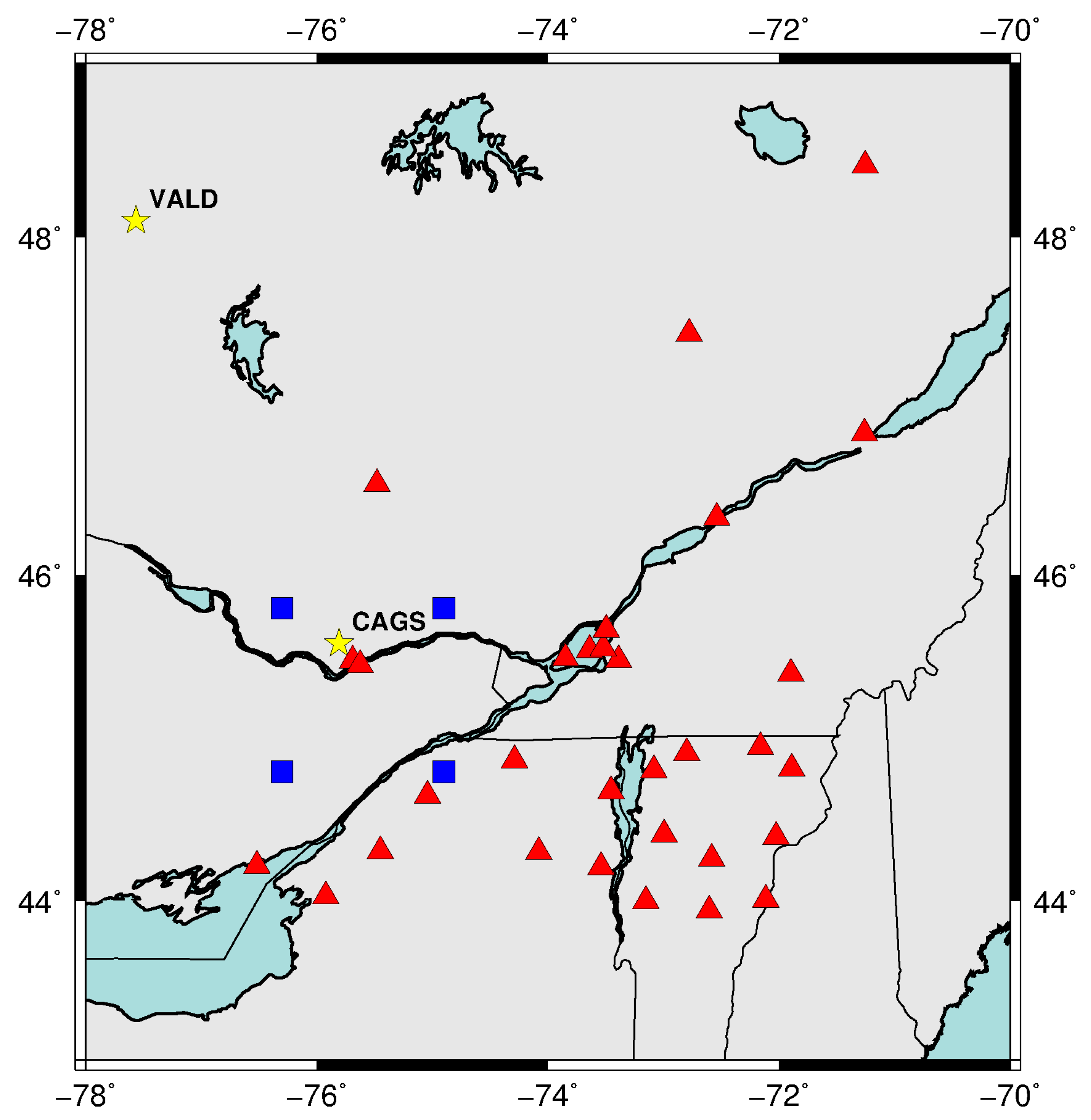
This section reviews the concepts presented in previous sections through a detailed example with real data. The area selected has an irregular station distribution with higher station density in the south coming from permanent reference stations located in the United States. The distribution of reference stations located in Canada is sparse with inter-station distances typically exceeding 200 km. Figure 1 shows reference stations with red triangles, and a hypothetical one-square grid is displayed in blue. Two test stations appear as yellow stars: VALD which is located outside of the convex hull formed by the network stations, and CAGS which is contained within the grid. The day processed for this analysis is 26 August 2018, which had some ionospheric activity at the beginning of the day (Kp > 7) before tapering off around midday for the region of interest.

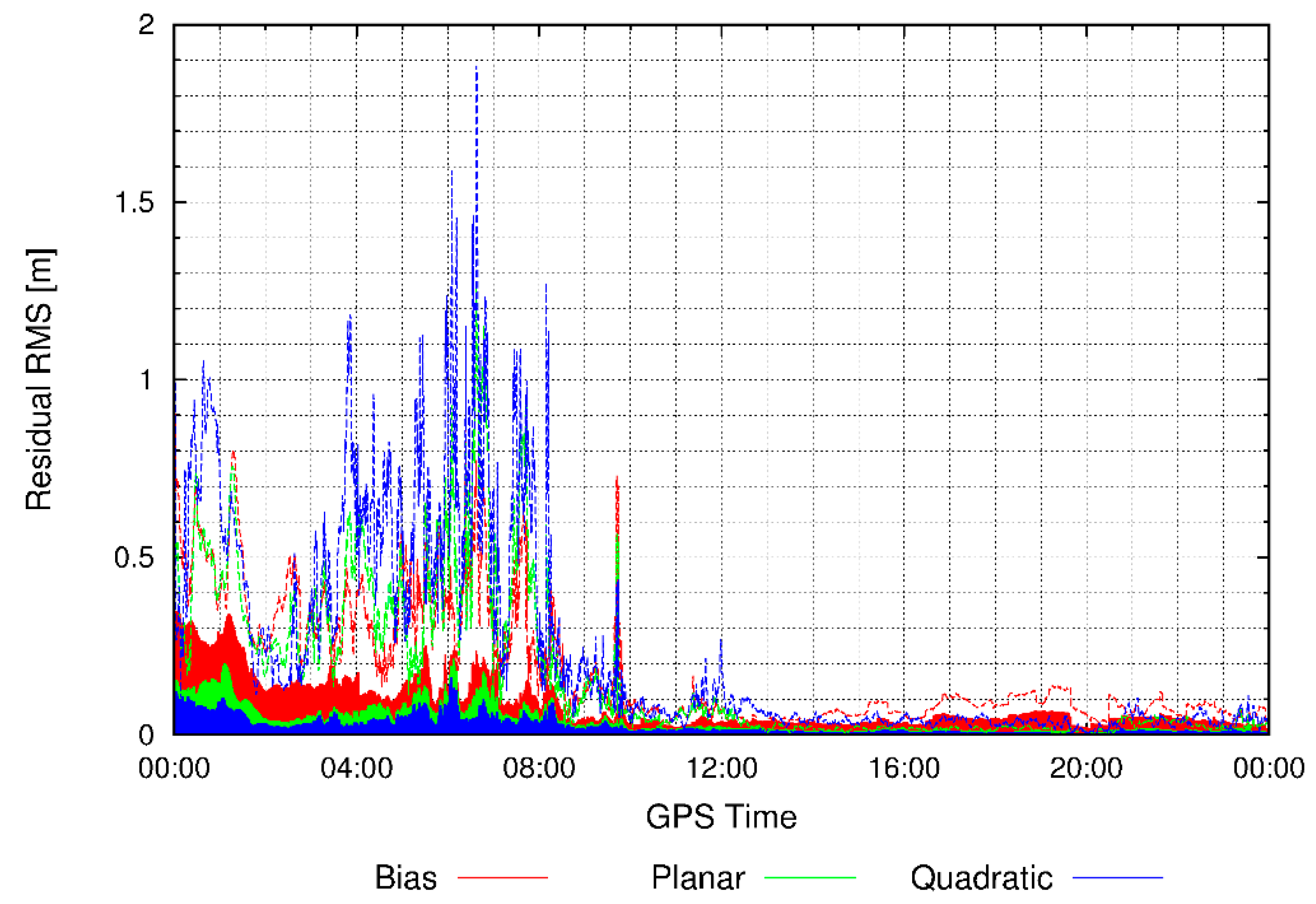
The choice of the mathematical model is influenced by its ability to correctly model the ionosphere. The three models tested in this study are the single-bias (6a), planar (6b), and quadratic (6c) models. Figure 2 shows, using vertical bars, the root-mean-square (RMS) residuals for all network stations at each epoch. As expected, adding parameters produces an improved fit and reduces residuals. However, increasing polynomial order is susceptible to causing edge effects, i.e., leading to larger residuals for stations that are outside of the network. This is illustrated using station VALD: the blue dashed line in Figure 2 illustrates that using the quadratic model results in several spikes in the residual RMS which are much larger than for other models. This concept is important as several grid points are located just outside of the network. Based on this information, the planar model is selected as the model of choice since it generally describes the ionosphere adequately while not being as affected by edge effects.

In the first iteration, slant ionospheric delays from PPP solutions are considered uncorrelated between stations, leading to a diagonal covariance matrix as defined in (10). As previously discussed, the receiver bias estimates are impacted by the mathematical model and the geometry of satellites observed at a station. To demonstrate this effect, Figure 3 presents the variation of receiver bias estimates between stations ALGO and ALG2, located approximately 70 m apart. Even though bias estimates contain ionospheric effects as described in (8), station proximity ensures that these errors are highly correlated. The red curve shows the receiver bias differences with a diagonal observation covariance matrix and the green curve displays the estimates when the signal covariance matrix is included in the adjustment, as per (19). Intra-day variations of phase biases are commonly observed [30] and are especially pronounced from 11:00 to 15:00. Additionally, the red curve shows amplified fluctuations between 08:00 and 13:00 as satellite G07 is discarded for station ALGO. Hence, considering correlations in the observation covariance matrix adds strength to the mathematical model and ensures greater consistency of the receiver bias estimates for nearby stations. In turn, adjustment residuals will better characterize the signal and lead to improved predictions.

The signal covariance matrix is defined based on the adjustment residuals from (11). Variograms are created on a satellite-by-satellite basis using up to 30 min of data: 15 min prior to and after the epoch of interest. As an example, Figure 4 shows the semivariances for satellite G32 at epoch 00:30 GPST, divided into 50 km bins. The density of points per pixel is represented by colors from blue (low density) to orange (high density). The 99th percentile value in each bin is displayed as an enlarged cyan dot. As explained in Equations (15) and (16), the bounded linear model shown in black is created by defining the sill from the largest 99th percentile value (in the 375 km bin), and using the largest gradient (in the 175 km bin) to compute the range. From these values, the circular variogram model of (17) is obtained and is displayed as a red curve in Figure 4.

Figure 5 provides an overview of the estimated sill values for all satellites tracked as a function of time. Each satellite is associated with a unique symbol/color combination. Satellite G32, introduced in the previous example, is depicted using empty cyan squares. At the epoch of interest (00:30), the sill exceeds 0.8 m², as illustrated in Figure 4. The sill values from Figure 5 demonstrate the higher ionospheric activity at the beginning of the day, followed by the very low activity from noon to midnight over this specific region. While the ionospheric prediction uncertainty at a grid point depends on its proximity to reference stations, it is almost guaranteed to be at the centimeter level past midday as the sill is consistently very small for all satellites.

With the functional and stochastic models defined, it is now possible to address the prediction capabilities. Figure 6 shows the slant ionospheric delay prediction error and its uncertainty for all satellites tracked by station CAGS over the 24-h period. Errors are approximated by removing, at every epoch, the mean value of the observed minus predicted delays to account for the receiver bias at CAGS. Figure 6a shows the prediction errors obtained from collocation, i.e., by interpolating delays directly from reference stations. The plot contains quasi-horizontal lines, depicting errors from satellites tracked at low elevation angles. As the satellite rises, errors become smaller but the uncertainty lags because it considers a window containing 30 min of data to define the variograms. Larger errors and uncertainties occurred earlier in the day, but most predictions for the second half of the day are at the millimeter to centimeter-level, as shown by the higher point density near to origin. The vast majority of points (>99.9%) fall above the diagonal black line, indicating that the uncertainty is larger than the prediction error. This result is deemed critical for the proper weighting of ionospheric constraints in the PPP filter. Figure 6b displays results obtained from predicting ionospheric delays at the four blue grid points and then interpolating these values back at the user position. As expected, there is an increase in errors and uncertainties associated with the double interpolation, but results are generally of similar quality and there is no reason to believe that creating a grid is significantly detrimental to the user.

Figure 7 shows GPS-only single-frequency PPP solutions computed at station CAGS. Even though it is a static reference station, no assumption is made regarding the receiver dynamics during processing. Slant ionospheric delays are estimated in the PPP filter with a process noise of 3 cm/√s, and constraints are applied from a GIM at the beginning of satellite arcs only. The top panel displays the solution without precise ionospheric constraints from the grid. Position estimates are noisy since carrier-phase observations lack the redundancy necessary to measure both the receiver displacement and slant ionospheric delays, and code observations contribute significantly to the solution. When adding precise ionospheric constraints from the grid (see Figure 7b), the additional redundancy allows for reduced noise in the position estimates, especially during the second half of the day when the sill values are much smaller according to Figure 5. During more disturbed periods (again refer to Figure 5), the uncertainties associated with the predictions are larger and the weaker constraints only reduce noise marginally. Over the 24-h period, RMS errors are reduced by more than 50% for all components.

8. Ionospheric Grid Evaluation

The concept of ionospheric grids is tested over Canada; specifically, only the southernmost part of the country is considered given the very sparse reference stations at higher latitudes. Figure 8 shows, as red triangles, stations available for the estimation of ionospheric corrections. From these stations, ionospheric estimates are computed, for all satellites in view, at grid points represented by squares in Figure 8. These grid points are depicted using various colors to distinguish zones, as previously discussed in this paper. The definition of these zones is not rigid: as a general guideline, a zone must include enough stations to determine a significant variogram, while being as small as possible to minimize model errors. In this study, a total of 10 zones have been defined, ranging from approximately 75,000 to 320,000 km². Due to the lack of reference stations in the center of the country, no grid points are included in this area. Distinct grid point spacings are implemented in each zone depending on station density. Grid points from adjacent zones typically overlap to offer continuous coverage since users can only interpolate ionospheric corrections from grid points belonging to a unique zone. For each zone, a box is defined from its outer grid points; this box is then extended by an additional grid square in each direction (north, south, east, west), and all stations lying within this extended box are selected as reference stations contributing to the ionospheric model. Users identified for positioning tests are not included as reference stations and are depicted as yellow stars.

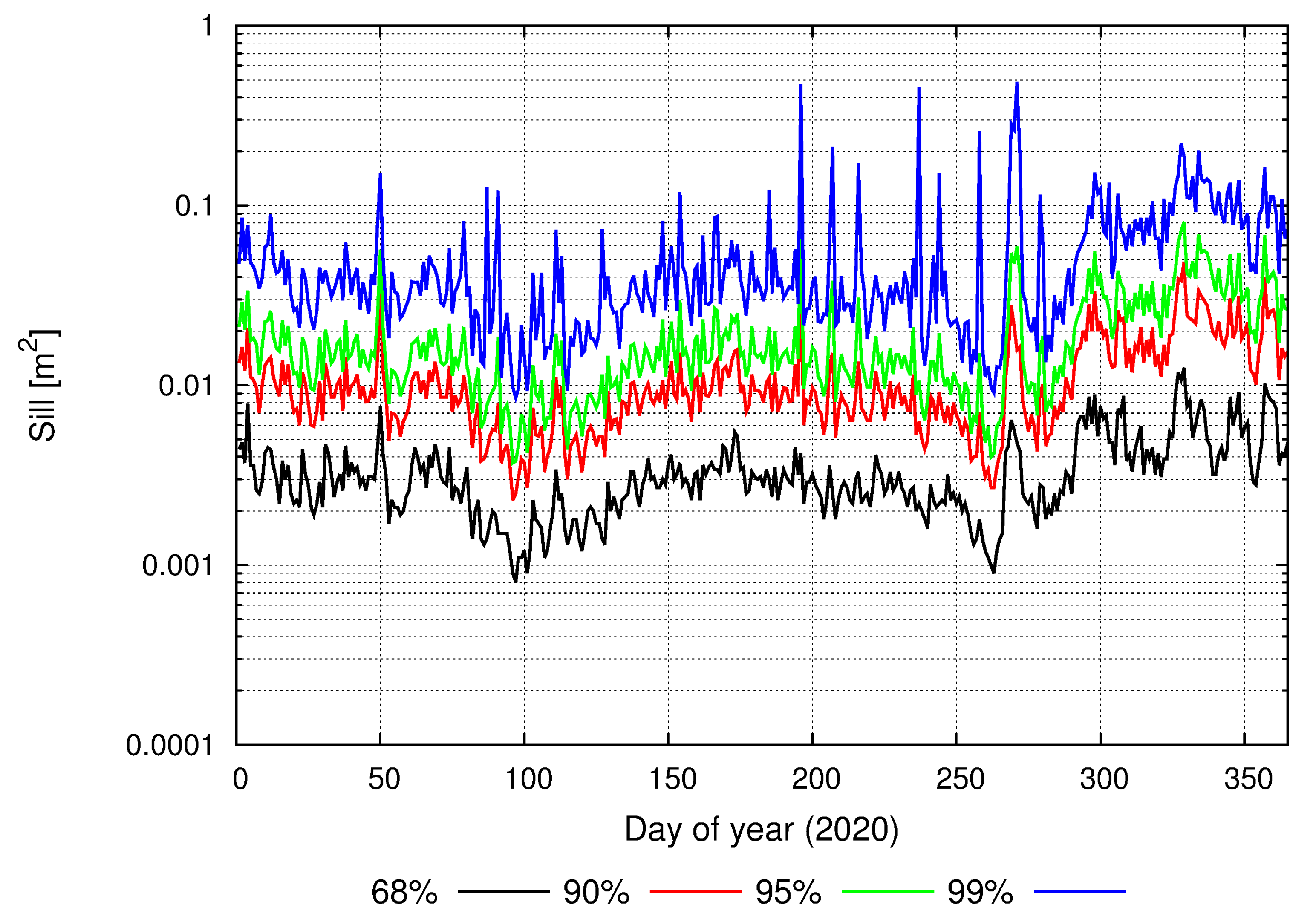
Ionospheric grids are computed daily for the year 2020, at an interval of 30 s, using the methodology described in this paper. Only satellites for which the elevation angle with respect to the zone centroid exceeds 15 degrees are included in the following analysis. Variograms are generated epoch-wise on a satellite-by-satellite basis to allow for a detailed characterization of the ionosphere. For each day of the year, all sill values are sorted and percentile values are identified as a means of evaluating ionospheric activity. Figure 9 shows the 68th, 90th, 95th, and 99th percentiles of the sill. Overall, few fluctuations occurred, indicating that 2020 was a year with little ionospheric activity. A few spikes are visible in the 99th percentiles, and they were found to be mostly associated with satellites tracked at a low elevation angle above the local horizon. Since the sill represents the variance of decorrelated samples, the uncertainty of the predicted ionospheric delays is likely to be much less than the square root of the sill, considering that the contribution from the mathematical model is typically small. Given this information, this figure lets us infer that uncertainties were around 5 cm at a 68% level, and approximately 10 cm at 90%.

Since ionospheric delays at grid points are determined independently for each zone, they contain a unique bias governed by the datum constraints, see (7) and (8). Yet, differencing the predicted values at two grid points within a zone cancels this bias and allows for a direct comparison of overlapping points between adjacent zones. On a daily basis, all possible overlap errors were computed, then divided by their reported uncertainties, and sorted to compute percentiles. Figure 10 displays these normalized overlap errors, using histograms built from daily percentile values. The plot indicates that reported uncertainties are very conservative, meaning that they overbound errors more than 99% of the time. This finding was expected given the modified methodology utilized to define variograms, based on the 99th percentile values rather than the mean in each bin. Despite being conservative, uncertainties are not overly large, as emphasized previously in Figure 9.

To assess grid performance in the positioning domain, PPP solutions from 31 stations are computed using 53 days in 2020 (every Wednesday of the year). The first hour of each day is processed using sessions of various durations, from 5 to 60 min. The IGS final orbits are used [34], along with an in-house clock combination preserving the integer nature of carrier-phase ambiguities at the user end [35]. Dual-frequency observations for both GPS and GLONASS are considered, although ionospheric grids are only available for GPS. Ambiguity resolution is attempted solely on GPS ambiguities observed for at least 5 min. Additional details on the PPP parameterization are presented in [36].

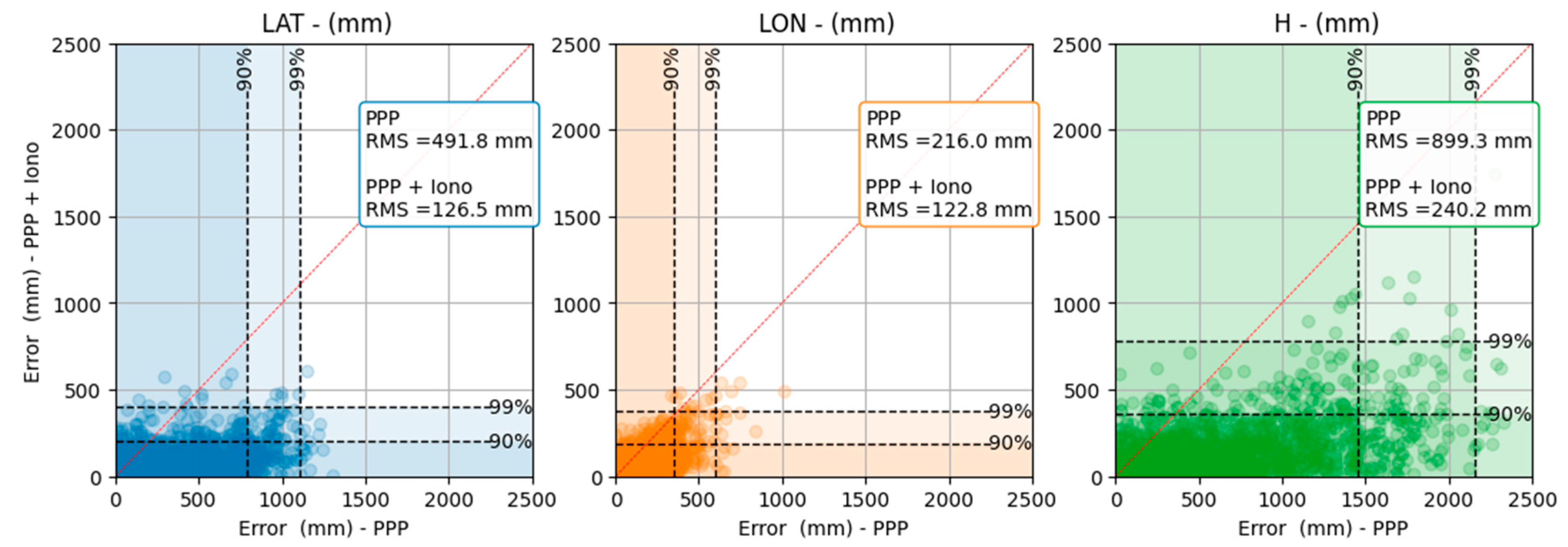
Figure 11 contains latitude, longitude, and height errors obtained from 1604 static sessions lasting 5 min (some sessions were discarded due to missing data). The figure compares solutions without (x-axis) and with (y-axis) the use of ionospheric grids. Points located below the diagonal line indicate that applying ionospheric constraints reduced positioning errors. Root-mean-square errors were reduced by 46%, 66%, and 39% for the latitude, longitude, and height components, respectively. The 90th and 99th percentile lines are also included as additional information. These statistics include stations from all zones, irrespective of the grid density.

Figure 11 also indicates that several sessions (<20%) experienced an increase in error with the addition of external ionospheric constraints. This phenomenon is possible in the presence of errors in the corrections. However, variograms ensure that corrections are associated with an inflated uncertainty. As such, the standard deviations from the PPP filter still adequately characterize positioning errors as shown in Figure 12. The RMS of the latitude and longitude standard deviations is around 36 and 38 cm, respectively, while it is 69 cm for the height. The RMS errors are about seven times smaller and never exceed the reported uncertainties for the datasets tested.

Figure 13 expands the 5-min sessions presented above to sessions of 10, 15, 20, 30, 45, and 60 min. From these results, an approximate convergence curve is interpolated. The impact of adding precise ionospheric corrections to dual-frequency PPP solutions is more significant for shorter sessions. As sessions get longer, carrier-phase ambiguities are naturally resolved without the need for ionospheric information. For this reason, improvements taper off slowly until they become almost negligible (in terms of absolute error) around the 30-min mark.

Precise ionospheric corrections are useful in speeding up the convergence time of dual-frequency datasets, but they play a more critical role with single-frequency receivers. Since the availability of low-cost receiver data across the country is limited, the same stations are processed using only signals from the GPS L1 band. While the results obtained are not representative of true low-cost equipment, they nonetheless provide a means of evaluating the impact of the ionospheric grids. Figure 14 shows results from 5-min sessions in static mode; note that ambiguity resolution is disabled for single-frequency data processing. Applying ionospheric constraints from the grids results in a decrease in RMS errors of 74%, 43%, and 73% in the latitude, longitude, and height components, respectively. Again, certain sessions experienced a slight increase in errors which, however, remains within the reported uncertainties.

The convergence of single-frequency datasets in static mode is displayed in Figure 15. Since geodetic-quality receivers are used, pseudorange noise is low and even solutions without precise ionospheric information eventually converge to cm-level accuracies. This convergence is significantly expedited with the use of ionospheric grids, reaching sub-dm level after about 20 min. Over the full hour, improvements remain relatively constant at over 60% for all components.

The last test compares the RMS errors of 24-h single-frequency kinematic PPP solutions with and without ionospheric grids, as previously shown in Figure 7. If available, precise ionospheric corrections are applied for all satellites at every epoch over the full day. Results are displayed in Figure 16, with each point representing the RMS value of a single 24-h session. The vast majority of datasets (>98%) are improved by ionospheric corrections, with RMS error reductions of 65%, 62%, and 59% for the latitude, longitude, and height components, respectively. Furthermore, ionospheric grids enable centimeter-level kinematic solutions in all components. Among the deteriorated solutions, all but six belong to two stations. The cause of these larger RMS errors was traced to the presence of small (1 cycle) undetected cycle slips: while they are partly absorbed by ionospheric parameters in the solution without grids, the tighter constraints provided by the external ionospheric corrections seem to push the errors into the position estimates. This issue will require further investigation.

9. Conclusions

Precise ionospheric corrections provide significant benefits to PPP users by enabling faster ambiguity resolution and reducing positioning errors. This paper presented a methodology for the generation of grid-based ionospheric corrections for wide areas, with a special emphasis on the uncertainties associated with these corrections.

Slant ionospheric delays at individual reference stations are first obtained from a PPP solution with ambiguities resolved. This approach leads to very precise estimates, albeit biased by a receiver-dependent term. To separate the receiver bias from the ionosphere, a mathematical representation of the ionosphere is needed. In this case, a wide area is divided into small zones and a satellite-specific planar model is adopted within each zone. Under undisturbed ionospheric conditions, the planar model adequately represents the ionosphere, while avoiding possible edge effects associated with higher-order polynomial functions.

From the model adjustment residuals, ionospheric conditions are measured in the form of satellite-specific variograms. The 99th percentile value in each distance bin is used as opposed to the mean value to obtain inflated uncertainties that overbound most errors. An experimental linear variogram is first computed to identify the range and the sill and, from these values, a circular variogram is then defined which further allows the characterization of spatial variations in two dimensions. These variograms, updated every epoch using 15 min of data prior to and after the epoch being processed, then serve to define a fully-populated observation covariance matrix leading to better parameter estimates such as receiver biases.

The variograms are then used to predict ionospheric delays at grid points, along with their uncertainties. Grids are computed at 30-s intervals for each satellite. PPP users obtain ionospheric corrections at their location by performing a bilinear interpolation from grid point estimates and, possibly, a temporal interpolation. To remove the presence of zone-specific biases in grid estimates, it is recommended to apply between-satellite single-differenced corrections at the user end.

The methodology presented was tested using 31 users, based on an hour of data over a period of 53 weeks in 2020. A variogram analysis showed that no major storms occurred in 2020, with a few larger sill values associated mostly with satellites observed at low elevation angles. As a coarse estimate, about 68% of ionospheric predictions in 2020 had an uncertainty of around 5 cm or better. The accuracy of dual-frequency PPP solutions was substantially improved, especially for sessions shorter than 30 min. RMS errors around the 5 cm mark can now be obtained from 5-min static sessions, down from 15 min without ionospheric corrections. Improvements are even more pronounced for geodetic-grade single-frequency data processing as RMS error reductions of around 70% are observed even for hour-long static sessions.

While multi-GNSS and multi-frequency data processing offers the possibility of rapid convergence to cm-level accuracy without precise ionospheric corrections, the latter is still useful to make instantaneous convergence more robust. Furthermore, the adoption of multi-frequency receivers by a majority of users will take time and precise ionospheric corrections over wide areas will enable more timely access to the global reference frame.

References

- Collins, P.; Bisnath, S. Issues in ambiguity resolution for precise point positioning. In Proceedings of the 24th International Technical Meeting of the Satellite Division of The Institute of Navigation (ION GNSS 2011), Portland, OR, USA, 20–23 September 2011; pp. 679–687. [Google Scholar]
- Li, X.; Zhang, X.; Ge, M. Regional reference network augmented precise point positioning for instantaneous ambiguity resolution. J. Geod. 2011, 85, 151–158. [Google Scholar] [CrossRef]
- Zhang, B.; Teunissen, P.J.G.; Odijk, D. A novel un-differenced PPP-RTK concept. J. Navig. 2011, 64, S180–S191. [Google Scholar] [CrossRef] [Green Version]
- Wübbena, G.; Schmitz, M.; Bagge, A. PPP-RTK: Precise point positioning using state-space representation in RTK networks. In Proceedings of the 18th International Technical Meeting of the Satellite Division of The Institute of Navigation (ION GNSS 2005), Long Beach, CA, USA, 13–16 September 2005; pp. 2584–2594. [Google Scholar]
- Hernández-Pajares, M.; Juan, J.M.; Sanz, J.; Orus, R.; Garcia-Rigo, A.; Feltens, J.; Komjathy, A.; Schaer, S.C.; Krankowski, A. The IGS VTEC maps: A reliable source of ionospheric information since 1998. J. Geod. 2011, 83, 263–275. [Google Scholar] [CrossRef]
- Rovira-Garcia, A.; Juan, J.M.; Sanz, J.; González-Casado, G.; Ibáñez, D. Accuracy of ionospheric models used in GNSS and SBAS: Methodology and analysis. J. Geod. 2016, 90, 229–240. [Google Scholar] [CrossRef]
- Banville, S.; Collins, P.; Zhang, W.; Langley, R.B. Global and regional ionospheric corrections for faster PPP convergence. J. Inst. Navig. 2014, 61, 115–124. [Google Scholar] [CrossRef]
- Rovira-Garcia, A.; Juan, J.M.; Sanz, J.; González-Casado, G. A worldwide ionospheric model for fast precise point positioning. IEEE Trans. Geosci. Remote 2015, 53, 4596–4604. [Google Scholar] [CrossRef] [Green Version]
- Psychas, D.; Verhagen, S.; Liu, X.; Memarzadeh, Y.; Visser, H. Assessment of ionospheric corrections for PPP-RTK using regional ionosphere modelling. Meas. Sci. Technol. 2019, 30, 014001. [Google Scholar] [CrossRef] [Green Version]
- Wanninger, L. Improved ambiguity resolution by regional differential modelling of the ionosphere. In Proceedings of the 8th International Technical Meeting of the Satellite Division of The Institute of Navigation (ION GPS 1995), Palm Springs, CA, USA, 12–15 September 1995; pp. 55–62. [Google Scholar]
- Sparks, L.; Blanch, J.; Pandya, N. Estimating ionospheric delay using kriging: 1. Methodology. Radio Sci. 2011, 46, RS0D21. [Google Scholar] [CrossRef]
- Sparks, L.; Blanch, J.; Pandya, N. Estimating ionospheric delay using kriging: 2. Impact on satellite-based augmentation system availability. Radio Sci. 2011, 46, RS0D22. [Google Scholar] [CrossRef]
- Blanch, J. Using Kriging to Bound Satellite Ranging Errors Due to the Ionosphere. Ph.D. Thesis, Stanford University, Stanford, CA, USA, 2003. [Google Scholar]
- Schaer, S.; Gurtner, W.; Feltens, F. IONEX: The IONosphere map Exchange format version 1. In Proceedings of the 1998 IGS Analysis Centers Workshop, ESOC, Darmstadt, Germany, 9–11 February 1998. [Google Scholar]
- QZSS Cabinet Office. Quasi Zenith Satellite System Interface Specification Centimeter Level Augmentation Service (IS QZSS L6 004); QZSS Cabinet Office: Tokyo, Japan, 14 July 2021. [Google Scholar]
- Vana, S.; Aggrey, J.; Bisnath, S.; Leandro, R.; Urquhart, L.; Gonzalez, P. Analysis of GNSS correction data standards for the automotive market. J. Inst. Navig. 2019, 66, 577–592. [Google Scholar] [CrossRef]
- Ciraolo, L.; Azpilicueta, F.; Brunini, C.; Meza, A.; Radicella, S.M. Calibration errors on experimental slant total electron content (TEC) determined with GPS. J. Geod. 2007, 81, 111–120. [Google Scholar] [CrossRef]
- Teunissen, P.J.G.; Khodabandeh, A. Do GNSS parameters always benefit from integer ambiguity resolution? A PPP-RTK network scenario. In Proceedings of the 27th International Technical Meeting of the Satellite Division of The Institute of Navigation (ION GNSS+ 2014), Tampa, FL, USA, 8–12 September 2014; pp. 590–600. [Google Scholar]
- Vollath, U.; Buecherl, A.; Landau, H.; Pagels, C.; Wagner, B. Multi-base RTK positioning using virtual reference stations. In Proceedings of the 13th International Technical Meeting of the Satellite Division of The Institute of Navigation (ION GPS 2000), Salt Lake City, UT, USA, 19–22 September 2000; pp. 123–131. [Google Scholar]
- Euler, H.J.; Keenan, C.R.; Zebhause, B.E. Study of a simplified approach in utilizing information from permanent reference station arrays. In Proceedings of the 14th International Technical Meeting of the Satellite Division of The Institute of Navigation (ION GPS 2001), Salt Lake City, UT, USA, 11–14 September 2001; pp. 379–391. [Google Scholar]
- Wübbena, G.; Bagge, A.; Schmitz, M. RTK networks based on Geo++® GNSMART–concepts, implementation, results. In Proceedings of the 14th International Technical Meeting of the Satellite Division of The Institute of Navigation (ION GPS 2001), Salt Lake City, UT, USA, 11–14 September 2001; pp. 368–378. [Google Scholar]
- Zha, J.; Zhang, B.; Liu, T.; Hou, P. Ionosphere-weighted undifferenced and uncombined PPP-RTK: Theoretical models and experimental results. GPS Solut. 2021, 25, 135. [Google Scholar] [CrossRef]
- Banville, S.; Langley, R.B. Defining the basis of an integer-levelling procedure for estimating slant total electron content. In Proceedings of the 24th International Technical Meeting of the Satellite Division of The Institute of Navigation (ION GNSS 2011), Portland, OR, USA, 19–23 September 2011; pp. 2542–2551. [Google Scholar]
- Zhang, B.C.; Ou, J.K.; Yuan, Y.B.; Li, Z.S. Extraction of line-of-sight ionospheric observables from GPS data using precise point positioning. Sci. China Earth Sci. 2012, 55, 1919–1928. [Google Scholar] [CrossRef]
- Odijk, D.; Zhang, B.; Khodabandeh, A.; Odolinski, R.; Teunissen, P.J.G. On the estimability of parameters in undifferenced, uncombined GNSS network and PPP-RTK user models by means of S-system theory. J. Geod. 2016, 90, 15–44. [Google Scholar] [CrossRef]
- Teunissen, P.J.G.; Khodabandeh, A. Review and principles of PPP-RTK methods. J. Geod. 2015, 89, 217–240. [Google Scholar] [CrossRef]
- Banville, S. Improved Convergence for GNSS Precise Point Positioning. Ph.D. Thesis, University of New Brunswick, Fredericton, NB, Canada, 2014. [Google Scholar]
- Sparks, L.; Komjathy, A.; Mannucci, A.J. Estimating SBAS ionospheric delays without grids: The conical domain approach. In Proceedings of the 2004 National Technical Meeting of The Institute of Navigation, San Diego, CA, USA, 26–28 January 2004; pp. 530–541. [Google Scholar]
- Zhang, B.; Teunissen, P.J.G.; Yuan, Y.; Zhang, X.; Li, M. A modified carrier-to-code leveling method for retrieving ionospheric observables and detecting short-term temporal variability of receiver differential code biases. J. Geod. 2019, 93, 19–28. [Google Scholar] [CrossRef] [Green Version]
- Zhang, B.; Teunissen, P.J.G.; Yuan, Y. On the short-term temporal variations of GNSS receiver differential phase biases. J. Geod. 2017, 91, 563–572. [Google Scholar] [CrossRef] [Green Version]
- Webster, R.; Oliver, M. Geostatistics for Environmental Scientists, 2nd ed.; John Wiley: New York, NY, USA, 2007. [Google Scholar]
- Moritz, H. Advanced Least-Squares Methods; Report No 175; Department of Geodetic Science, Ohio State University: Columbus, OH, USA, 1972. [Google Scholar]
- Krakiwsky, E.J. A synthesis of Recent Advances in the Method of Least Squares; Lecture Notes 42; Department of Geodesy and Geomatics Engineering, University New Brunswick: Fredericton, NB, Canada, 1975. [Google Scholar]
- Johnston, G.; Riddell, A.; Hausler, G. The international GNSS service. In Springer Handbook of Global Navigation Satellite Systems, 1st ed.; Teunissen, P.J.G., Montenbruck, O., Eds.; Springer International Publishing: Berlin, Germany, 2017; pp. 967–982. [Google Scholar] [CrossRef]
- Banville, S.; Geng, J.; Loyer, S.; Schaer, S.; Springer, T.; Strasser, S. On the interoperability of IGS products for precise point positioning with ambiguity resolution. J. Geod. 2020, 94, 10. [Google Scholar] [CrossRef]
- Banville, S.; Hassen, E.; Lamothe, P.; Farinaccio, J.; Donahue, B.; Mireault, Y.; Goudarzi, M.A.; Collins, P.; Ghoddousi-Fard, R.; Kamali, O. Enabling ambiguity resolution in CSRS-PPP. J. Inst. Navig. 2021, 68, 433–451. [Google Scholar] [CrossRef]
Figure 1.
Test network represented with red triangles, grid points are in blue, and stations CAGS and VALD are not part of the network and are used to test ionospheric predictions.
Figure 2.
Epoch-wise residual RMS for network stations (vertical bars) and station VALD (dashed lines) located outside of the network.
Figure 3.
Variation of receiver DCB difference between stations ALGO and ALG2 with a diagonal and fully-populated observation covariance matrix.
Figure 4.
Process of creating a fitted overbound for the 99th percentile of semivariances.
Figure 5.
Estimated variogram sill on an epoch-by-epoch basis for all satellites seen by the network.
Figure 6.
Prediction errors and their uncertainties at station CAGS: (a) directly from collocation; (b) interpolated from grid points.
Figure 7.
Single-frequency pseudo-kinematic PPP positioning errors for station CAGS: (a) without ionospheric constraints; (b) with gridded ionospheric constraints. RMS errors for each component are provided in the legend.
Figure 8.
Ionospheric grid in southern Canada. Red triangles represent reference stations, squares are grid points, and stars are users. Zones are distinguished using grid points of different colors.
Figure 9.
Variogram sill percentiles estimated daily in 2020.
Figure 10.
Normalized overlap errors between zones in 2020.
Figure 11.
Impact of ionospheric grids on 5-min dual-frequency PPP-AR static solutions.
Figure 12.
Error vs reported uncertainty for 5-min dual-frequency PPP-AR static solutions using ionospheric grids.
Figure 13.
Impact of ionospheric grids on dual-frequency PPP-AR convergence of static solutions.
Figure 14.
Impact of ionospheric grids on 5-min single-frequency PPP-float static solutions.
Figure 15.
Impact of ionospheric grids on single-frequency PPP-float convergence of static solutions.
Figure 16.
Impact of ionospheric grids on 24-h single-frequency PPP-float kinematic solutions.
Publisher’s Note: MDPI stays neutral with regard to jurisdictional claims in published maps and institutional affiliations. |
© 2022 by the authors. Licensee MDPI, Basel, Switzerland. This article is an open access article distributed under the terms and conditions of the Creative Commons Attribution (CC BY) license (https://creativecommons.org/licenses/by/4.0/).
Share and Cite
MDPI and ACS Style
Banville, S.; Hassen, E.; Walker, M.; Bond, J. Wide-Area Grid-Based Slant Ionospheric Delay Corrections for Precise Point Positioning. Remote Sens. 2022, 14, 1073. https://0-doi-org.brum.beds.ac.uk/10.3390/rs14051073
AMA Style
Banville S, Hassen E, Walker M, Bond J. Wide-Area Grid-Based Slant Ionospheric Delay Corrections for Precise Point Positioning. Remote Sensing. 2022; 14(5):1073. https://0-doi-org.brum.beds.ac.uk/10.3390/rs14051073
Chicago/Turabian StyleBanville, Simon, Elyes Hassen, Micah Walker, and Jason Bond. 2022. "Wide-Area Grid-Based Slant Ionospheric Delay Corrections for Precise Point Positioning" Remote Sensing 14, no. 5: 1073. https://0-doi-org.brum.beds.ac.uk/10.3390/rs14051073
Note that from the first issue of 2016, this journal uses article numbers instead of page numbers. See further details here.