
Efficient Depth Fusion Transformer for Aerial Image Semantic Segmentation


1
School of Geodesy and Geomatics, Wuhan University, Wuhan 430079, China
2
School of Computer Science, Wuhan University, Wuhan 430072, China
*
Author to whom correspondence should be addressed.
Remote Sens. 2022, 14(5), 1294; https://0-doi-org.brum.beds.ac.uk/10.3390/rs14051294
Submission received: 13 February 2022
/
Accepted: 3 March 2022
/
Published: 7 March 2022
(This article belongs to the Topic High-Resolution Earth Observation Systems, Technologies, and Applications)
Abstract
:Taking depth into consideration has been proven to improve the performance of semantic segmentation through providing additional geometry information. Most existing works adopt a two-stream network, extracting features from color images and depth images separately using two branches of the same structure, which suffer from high memory and computation costs. We find that depth features acquired by simple downsampling can also play a complementary part in the semantic segmentation task, sometimes even better than the two-stream scheme with the same two branches. In this paper, a novel and efficient depth fusion transformer network for aerial image segmentation is proposed. The presented network utilizes patch merging to downsample depth input and a depth-aware self-attention (DSA) module is designed to mitigate the gap caused by difference between two branches and two modalities. Concretely, the DSA fuses depth features and color features by computing depth similarity and impact on self-attention map calculated by color feature. Extensive experiments on the ISPRS 2D semantic segmentation dataset validate the efficiency and effectiveness of our method. With nearly half the parameters of traditional two-stream scheme, our method acquires 83.82% mIoU on Vaihingen dataset outperforming other state-of-the-art methods and 87.43% mIoU on Potsdam dataset comparable to the state-of-the-art.
1. Introduction
Semantic segmentation is a fundamental task in remote sensing and aims at assigning a semantic label to each pixel. Most of the existing semantic segmentation networks are based on the seminal work [1], a fully convolutional network (FCN). The standard paradigm of an FCN model has an encoder–decoder architecture: The encoder learns feature representation, while the decoder classifies features in a pixel level.
Although those FCN methods have achieved good results, there exists the problem of induction bias in the process of image feature extraction, mainly caused by the weight sharing mechanism of Convolution Neural Network (CNN) and local characteristics of convolution operators. Convolution is insensitive to the global position of the feature and only takes a small pixel region as input. In order to obtain the long-range dependence of features, the pixel receptive field should be enlarged as much as possible. The proposal of residual connection [2] and dilated convolution [3] alleviates this problem to a certain extent, but it leads to the decrease in computational efficiency or the loss of details. Vision Transformer [4], a network architecture based on self-attention, completely solves this problem as self-attention computes on the whole image. At the same time, due to the particularity of the form of self-attention calculation, the network does not need too many parameters, and the training speed is faster. For the above reasons, the segmentation method based on Transformer has achieved better results than the CNN method, and its potential has not been tapped yet.
On the other hand, the availability of point cloud acquired by Lidar or Photogrammetry makes it possible to label an aerial image with additional elevation information. One way to utilize the point cloud is to produce Digital Surface Models (DSM) or normalized Digital Surface Models (nDSM) first [5,6]. Then, DSM is treated as a depth image, and thus the problem converts to an RGB-D semantic segmentation problem, helping to distinguish those ground objects that are easy to be confused with only appearance. However, fusing depth into an existing semantic segmentation network is not trivial. Simply stacking color and depth images together and inputting them to the network usually obtains an unsatisfactory result [7].
Most works considering depth adopt a two-steam style [8,9,10,11,12,13,14]. Color images and depth maps are fed separately into two branches with the same structure, and the learned features are fused in the encoder or decoder phase. It is obvious that the later features are to fuse, the more parameters and more computation are needed, as two branches double the cost. There comes an urgent need to fuse depth information in a lightweight manner. Moreover, color images contain more information than depth mapa, and their internal information types are different. It is reasonable to treat depth maps differently. Meanwhile, the depth map of a single view has limited power in presenting geometric features. It may be better to use depth as an aid to color image segmentation.
Depth-aware CNN [15] designs the variant convolution and pooling modules to take depth into account and do not introduce any parameters and computation complexity to the conventional CNN. It is a feasible direction to solve the computational problem, but several limitations exist. Firstly, the convolution operator computes on a fixed sized window and thus can only fuse local depth information. Secondly, it is restricted to CNN methods, and there remains space to explore the nowadays prevalent transformer network. Thirdly, it and its following works [16,17,18] represent a trend to fuse depth in a handcraft design, which loses the advantages of a two-stream scheme and is not easy to cooperate with existing 2D networks. In order to extend those RGB segmentation networks to RGB-D, we should replace convolution with the variant in the special locations which include extra hyperparameters.
To overcome the aforementioned challenges, the proposed method still adopts different branches to ease the burden on depth feature extraction, while still using the two-stream scheme to ensure the network’s simplicity and flexibility. The depth-aware CNN’s success reveals the probability of fusing depth features without too much extraction from depth maps, which enlightens us on the design of a lightweight depth branch. In the presented model, a simple image downsampling strategy through patch merging [19] is adopted to form a multiscale structure and meanwhile maintain information by extending channel numbers. Furthermore, in order to mitigate the gap caused by the different structures of the branches, a novel depth-aware self-attention module is designed, which is able to fuse depth in a global context.
In this paper, our main contributions can be summarized as follows:
- Differing from conventional two-stream networks of the same two branches, in order to improve the computational efficiency, our network adopts two different branches, which includes a novel depth branch of four downsampling convolution layers.
- Two kinds of self-attention module are proposed to mitigate the gap caused by teh difference between two branches and two modalities. We validate their capability and flexibility on the problem of multi-modal feature fusion.
- With the above two designs and the backbone transformer, we propose a more efficient network for RGB-D semantic segmentation task: Efficient Depth Fusion Transformer (EDFT).
The code is published at https://github.com/h1063135843/EDFT accessed on 1 March 2022.
2. Related Works
Concerning the proposed transformer network model for RGB-D segmentation tasks and the attention module for color and depth features fusion, this section discusses the related works from three aspects:
2.1. Acquiring Long-Range Dependency
Limited by the characteristics of convolution, a pixel can only perceive a small area around it, which is not good for segmentation. Statistically, Sun found that the central pixels on a patch could obtain higher classification accuracy than the edge areas [20]. Because of the padding and pooling operations, the pixels of edge areas have smaller receptive fields.
In CNN methods, deeper layers or bigger kernels are usually adopted to enlarge the receptive fields. Under the balance between the size of receptive field and the computation cost, how to improve the interaction ability of pixel features in the decoder phase becomes important, which can indirectly expand the receptive field. By imitating the channel attention mechanism [21], S-RA-FCN [22] designed a spatial relation module to capture global spatial relations. Furthermore, HMANet [23] introduced class information to this process of spatial interaction.
Self-attention could also be applied in the decoder phase to interact with the features, which, however, comes with a high computational cost. Li reduced the time complexity of the computation by exchanging matrix multiplication order through linearization [24]. HMANet [23] introduced a region shuffle attention module to improve the efficiency of the self-attention mechanism through reducing redundant features and forming region-wise representations.
With the development of computer vision and its related problems being solved, the transformer-based network can use self-attention to obtain receptive fields as large as the whole image. In the transformer-based network, self-attention is treated as the main operation in the encoder phase and not only as a single module in the decoder phase. References [25,26] applied a transformer model on remote imagery successfully. However, they only considered color features as inputs. The performance of the transformer on an RGB-D segmentation task also needs to be evaluated.
2.2. RGB-D Segmentation by Deep Learning
According to the fusion position, an RGB-D segmentation network can be partitioned into three categories [27]. Usually, the stack scheme is considered as early fusion [1,5,28,29,30,31], while the two-stream scheme fusing depth in the encoder phase tends to be middle fusion [8,9,10,11,12] and in the decoder phase to be late fusion [13,14]. Chen et al. [28] adopted early fusion but acquired promising results by learning two features independently with group convolution. The article [8] compared these three categories and drew the conclusion that middle fusion could improve segmentation accuracy by jointly learning stronger multi-modal features, while late fusion can recover errors from those pixels easy to be confused by a single modality.
Although middle fusion and late fusion could achieve satisfactory results from the perspective of accuracy, they are not efficient enough. Hence, in this paper, we design a lightweight depth branch to extract depth information.
2.3. Attention for RGB-D Fusion
Concerning the RGB-D segmentation problem, both the fusion position and fusion strategy are taken into consideration. Performing concatenation or adding operations to fuse color and depth is an equal-weight score fusion, ignoring the varying distributions of color and depth on different categories. A channel attention mechanism was introduced by SENet [21] and used to perform feature recalibration. It models the importance of different channels by squeezing the feature map to a 1D vector and selectively emphasizing informative features by multiplication of importance vector and original feature. Related researchers also applied channel attention module (CAM) for RGB-D fusion problem [10,12]. While CAM-DFCN [12] employs CAM solving both RGB-D fusion and multiscale feature fusion with concatenation of inputs, ACNet [10] recalibrate color and depth separately and forms a third virtual branch similar to [8]. Channel attention selects features from color and depth from the channel perspective, but it lacks the global contrast to two modalities. LSD-GF designed a gated fusion layer to weight color and depth on the whole and adjust the contributions of RGB and depth over each pixel [13]. SA-Gate [11] combined the gate design with channel attention and spatial attention bidirectionally and demonstrated impressive performance.
Self-attention’s success in both fields of computer vision and natural language processing shows its ability of feature modeling in different modalities. Inspired by this, in this paper, we introduced it into the RGB-D fusion process. Furthermore, two kinds of DSA are designed and compared to decide whether the global weighting paradigm or channel weighting paradigm performs better through an ablation study.
3. Method
This section describes the proposed DSA module and the network architecture of Efficient Depth Fusion Transformer (EDFT). EDFT is a two-steam style network with different branches, and the color branch is a transformer encoder, while the depth branch consists of only four convolution layers. DSA modules fuse color and depth features, and then output multistage features to a lightweight All-MLP (multi-layer perceptron) decoder adopted in Segformer.
3.1. Network Architecture
Firstly, the Segformer [32] used as our baseline method is briefly introduced. Then, a conventional two-stream scheme to handle RGB-D input is designed and explained. Finally, we improve the two-stream scheme and propose the EDFT to achieve both high accuracy and efficiency.
3.1.1. Segformer Network
In this section, towards a better understanding of our baseline method, the features of Segformer are clarified.
Segformer adopts an encoder–decoder architecture. The encoder is a hierarchical transformer and generates multiscale and multistage features like most CNN methods. There is a series of encoders, Segformer-B0 to Segformer-B5, with the same size outputs but different depth of layers in each stage. The decoder consists of only MLP layers and fuses multi-level features. Due to its simplicity and efficiency, the Segformer is chosen as our baseline method. In addition, it is also very convenient for other transformer backbones to be adapted to our proposed network.
Segformer does not use position embedding to introduce local information, but uses Mix-FFN and overlapped patch merging instead. Mix-FFN insert a 3 × 3 Convolution between two layers of MLP in the feed-forward network. Overlapped patch merging unifies the formal of the patch operations such as patch embedding and patch merging, both of which could be performed by the convolution of odd kernel sizes.
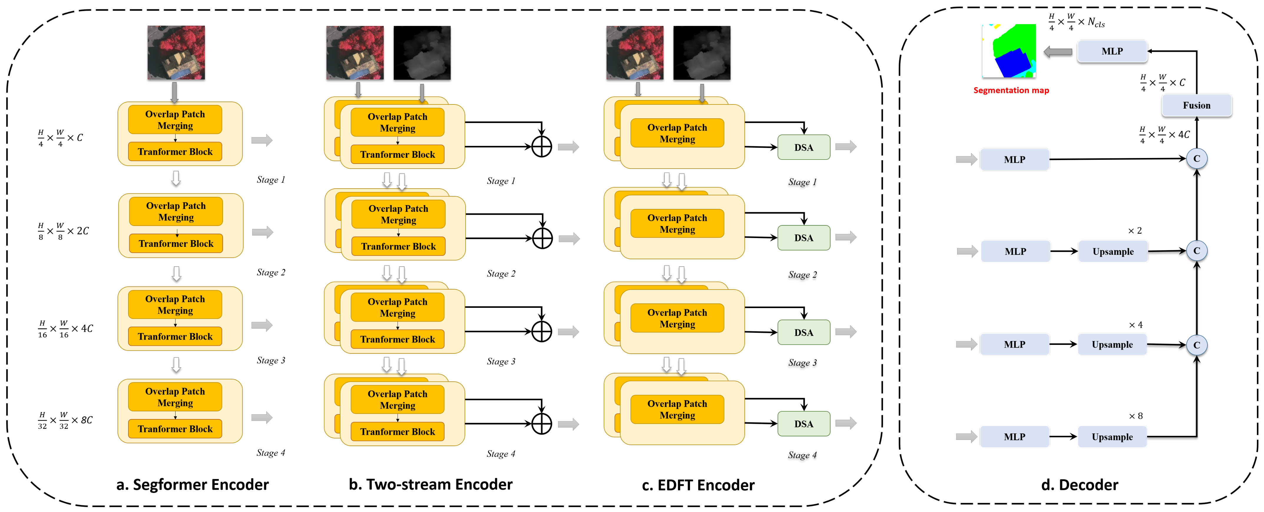
Input image sizes of H × W × 3 (or 1) are embedded to feature sizes of after the first overlapped patch merging module, where C is the embedding dimension. Take an input feature size of h × w × c, for example: The other three overlapped patch-merging modules output a feature size of . The word “overlap” represents the odd kernel size of the convolution, and it helps the transformer consider local information. The encoder in Figure 1a and the decoder in Figure 1d form the Segformer network.
3.1.2. Conventional Two-Stream Scheme
As simple stacking color and depth input can’t get satisfactory results, it is better to adapt Segformer to a two-stream network, fusing depth information in the encoder phase or decoder phase.
According to [8], the network adopts a middle fusion strategy and fuses color and depth features in the encoder phase to obtain a higher accuracy. Therefore, the network consists of two encoders and one decoder. The only difference between the two encoders lies in the first convolution layer, as color and depth inputs have different channels. Simple addition operation fuses two kinds of features in the same stage.
Moreover, where to fuse features in the encoder phase also needs to be decided. For the SegNet-like [33] network whose encoder outputs only the last stage feature, it is better to use the FuseNet [9] architecture, which passes the fused features in the previous stage to the next stage. However, our baseline method is a UNet-like [34] network whose encoder has multi-stage outputs. We argue that maybe it is better to pass the fused features to the decoder directly after the fusion process, as introducing depth information to color feature learning too early could harm the forming process of multiscale features. The encoder in Figure 1b and the decoder in Figure 1d form the Two-Stream Segformer network to handle the RGB-D segmentation task.
3.1.3. EDFT Network
To fuse depth information in a lightweight manner, a novel EDFT Network is proposed, which is a two-stream network with two different branches. It is reasonable for the two branches to adopt different structure, as color and depth modalities are complementary as they contain different kinds of information.
In Depth-Aware CNN [15], the pixel weight in the convolution process is determined by the trained parameter and difference between its corresponding depth and the center pixel’s depth. To keep a one-to-one mapping between color feature and original depth map, the depth map should be downsampled at the same time the color feature’ resolution decreases. We add a branch handling depth with a downsampling module to the existing RGB network explicitly and use overlap patch merging to downsample the image; meanwhile, we maintain information that may be lost in the downsampling process. Furthermore, it provides convenience for the following fusion process, as the depth branch outputs features the same size as the color branch.
We evaluate the experimental performance of the model with depth branch consisting of only downsample modules, which uses add operation to fuse features. This kind of model is denoted as “two-stream-differ” in this paper, while the conventional two-stream model is denoted as “two-stream-same”. As the experimental result shows, it is also beneficial for improving the model accuracy to fuse depth features only extracted by patch merging, and the “two-stream-differ” is even better than the “two-stream-same” in some situations. Nonetheless, it is also sometimes worse than the “two-stream-same”.
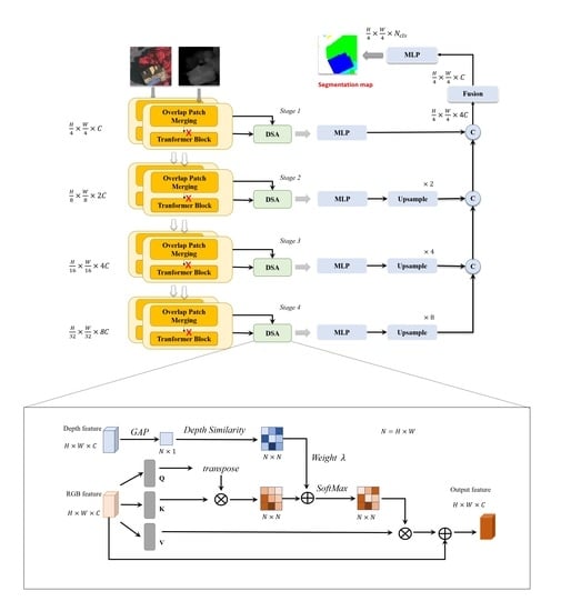
To make the best use of two kinds of features and mitigate the gaps between different branches and modalities, we propose the depth-aware self-attention module and replace simple addition with it to fuse features. The encoder in Figure 1c and the decoder in Figure 1d form our proposed EDFT network for RGB-D segmentation tasks.
3.2. Depth-Aware Self-Attention Module
Owing to the flexibility of similarity measurement, self-attention mechanism is very suited to fusing multi-modal features (not only between color and depth). Self similarity in each modality is computed first, and then the results of similarity measurements are combined to acquire a complex similarity considering two sides. It fuses features of different properties and different categories easily, which assign the Transformer the ability of very powerful joint feature modeling. Leveraging advantages of different data sources, the model can achieve higher accuracy and reliability.
In this section, the computation of self-attention is introduced first, and then two ways to cooperate depth into self-attention computation are explored.
3.2.1. Computation of Self-Attention
Given a feature F of size h × w × c, self-attention first reshapes it into an n × c vector, where n = h × w is the pixel number. Then, three linear layers project the input feature to the query, key, and value matrices, which have the same dimensions as the input:
where are the learned weight matrices of three linear layers, and F is the input feature of self-attention.
Query and key perform a dot product operation to measure similarity between two pixels i and j along channel dimension: , where means the ith column vector of query matrix Q in Equation (1), and means the jth column vector of key matrix K.
Similarity is scaled by a factor, the square of channel dimension, and normalized by softmax operation on account of all pixels to generate the contribution of pixel i to pixel j : , where c is the dimension of the input feature. The final result of computation is a weighted sum of value matrices: , where means the jth column vector of value matrix V in Equation (1).
The above process of computing self-attention could be written in the format of matrix multiplication:
where Q, K, V is calculated by Equation (1), and c is the dimension of the input feature.
3.2.2. Fusing Depth in a Concat Mode
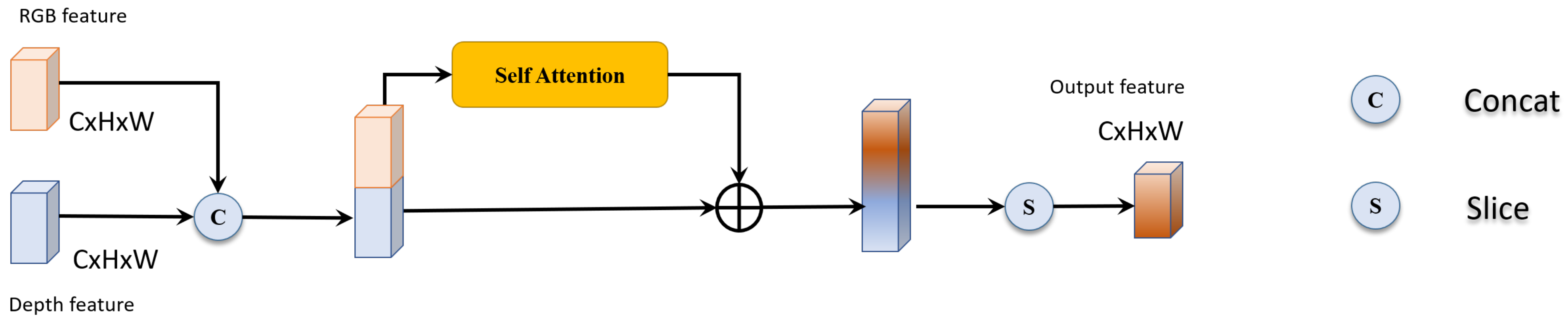
This subsection describes the module DSA-concat. There is a simple but effective solution to take consideration of depth during the process of computing self-attention. By concatenating color feature C and depth feature D and taking the concatenation result as input F, it extends the feature from the channel perspective, leverages the channel interaction of self-attention mechanism, and reaches the goal of fusing the two features.
As illustrated in Figure 2, residual learning is used to propagate better, preventing from gradient vanish. Furthermore, we slice the output and fetch only the front half part corresponding to the input color feature. It is designed for the purpose of considering depth features as a complementary data source. The computation of depth-aware self-attention in a concat mode could be depicted by the following formula:
where C is the input color feature, and D is the input depth feature. SA is the abbreviation of self-attention depicted in Section 3.2.1, and it equals to Equations (1) and (2).
3.2.3. Fusing Depth in an Addition Mode
This subsection describes the moudle DSA-add. Although we use slice operation to highlight color features, DSA-concat still lacks discriminatory actions over color and depth in a global manner. We propose a more lightweight and more flexible module to handle this problem.
As known to us, the core of self-attention mechanism lies in the similarity measurement. However, inner product by which color measures similarity may not be suited for depth. On intuition, the absolute difference between two pixels’ depth can measure the similarity: , where means the depth of pixel i. The minus sign ensures that pixels of closer depth are more similar. In addition, depth similarity could be also regarded as the subtraction format of vector attention [35]. Then, a weight coefficient is applied to balance color and depth items in the formula of composite similarity measurement:
where means the ith column vector of query matrix Q in Equation (1), and means the jth column vector of key matrix K. is the depth of pixel i, and is a weight coefficient.
To obtain the depth difference between two pixels from a depth feature of size h × w × c, global average pooling (GAP) operation [36] along channel dimension is used to restore depth features to size of h × w × 1. Then, the feature is reshaped to an n × 1 vector, and copied n times to expand into an n × n matrix . These processes ensure that depth similarity measurement could be depicted in matrix format, which is vital for acceleration. Depth-aware self-attention in an addition mode is illustrated as Figure 3 and computed as:
where ∘ means the functional composite operation. Q, K, V is calculated by Equation (1). D is the input depth feature, and is an intermediate format of depth feature.
4. Experiments
To validate the proposed network, we conduct comprehensive experiments on ISPRS Semantic Labeling Contest (2D) (http://www2.isprs.org/commissions/comm3/wg4/semantic-labeling.html (accessed on 27 May 2021)). The experimental results demonstrate that EDFT achieves comparable performance to the state-of-the-art on two datasets. This section first introduces experimental settings such as experimental datasets, accuracy metrics, and some implementation details. Then, the efficiency and effectiveness of the model are verified over two datasets. A series of experiments are conducted to study the effect of different modules and different parameters.
4.1. Experimental Settings
4.1.1. DataSets
ISPRS Semantic Labling Contest (2D) contains two image datasets acquired over Vaihingen and Potsdam (two citys in Germany), consisting of very high-resolution aerial images, corresponding DSMs, and ground labeling truth. Each pixel in the image is assigned to the one of six classes: impervious surface, building, low vegetation, tree, car, and clutter. To reduce the impact of uncertain border definitions on the evaluation, we use the annotation with eroded boundary provided by the organizer and ignore the eroded areas during evaluation.
Vaihingen Dataset has 16 training images and 17 testing images, following the previous works [22,23,29,30,31,37]. Images are resized to the average size of 2048 × 1536, and randomly cropped into images with a size of 256 × 256 when training. The Potsdam Dataset has 24 training images and 14 testing images. All are images have a size of 6000 × 6000. To save the loading time in the training phase, images are parted into 2000 × 2000 tiles and randomly cropped into 512 × 512 to augment data.
Both datasets provide DSM data extracted from the Lidar point cloud. In all experiments, we only use nDSM and treat it as a depth image. On the Vaihingen dataset, we use nDSM from [38], while on the Potsdam dataset, we use that from ISPRS official.
4.1.2. Metrics
All models are evaluated based on the pixel-based confusion matrices. Confusion matrices represent counts from predicted values in the column direction and the actual values in the row direction. The True Positives (TP) are the pixels on the main diagonal. The False Positive (FP) is the accumulation per column, excluding the main diagonal element, while the False Negative (FN) is along the row.
From the TPs, FPs, and FNs per class, the following measures are derived: Recall, Precision, F1 score, Intersection over Union (IoU), and Overall Accuracy (OA). They are defined as follows:
where , and N is the number of all pixels. OA is evaluated over a whole image, while F1 and IoU are evaluated for a specific class. Mean F1 and mIoU are the average of those for the six classes.
4.1.3. Implementation Details
Segformer in mmseg (https://github.com/open-mmlab/mmsegmentation.(accessed on 26 August 2021)) is utilized as our baseline method for its simplicity and efficiency. All experiments are conducted on a single GeForce RTX 3090. Most experimental settings are the same as the original Segformer, but several following parameters differ. We train the model for 80k iterations and set the batch size to 2. The normalization parameters are acquired by statistics from corresponding datasets, as color data contain IR bands and there is no reference for depth. PhotoMetric distortion is discarded as it is not suitable for depth. We test images with a sliding window size of 256 × 256 for the Vaihingen dataset and 512 × 512 for the Potsdam dataset, as remote images have the higher resolution.
4.2. Compare to the State-of-the-Art
4.2.1. Efficiency Contrast
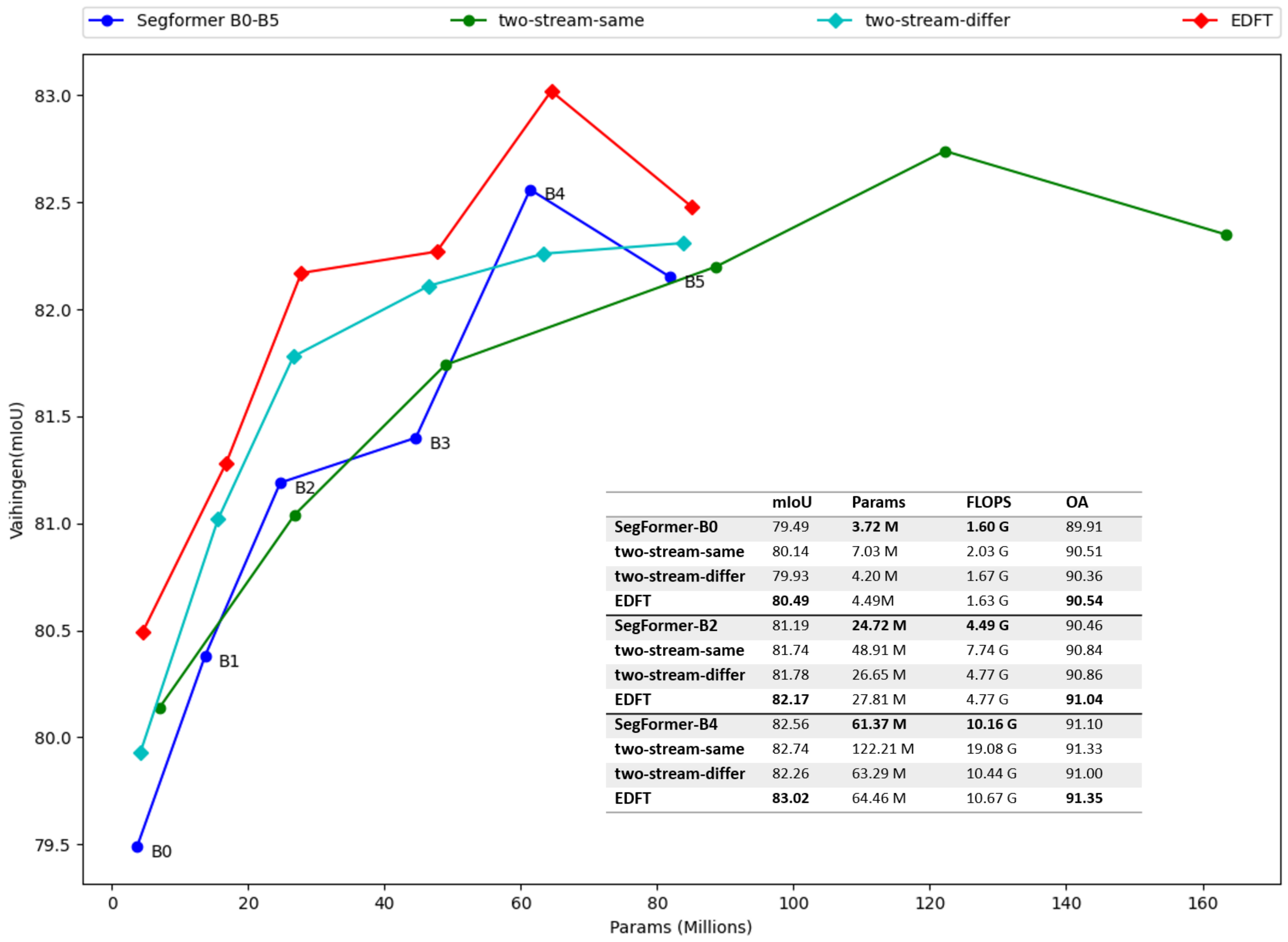
To verify the universality and efficiency, the baseline models of different sizes (from B0 to B5) are adapted according to the proposed method presented in this paper and measured by Params, GFlops, and other accuracy metrics. The results are shown in Figure 4. As shown in the figure, “two-stream-differ” and EDFT network using only the downsampling module can only increase the computational cost and the number of parameters by a fixed small value, unlike the “two-stream-same”, which increases by nearly two times. On the whole, the accuracy of the “two-stream-differ” is higher than that of the baseline method and lower than that of the “two-stream-same”, but in some cases, the results are the opposite (B2 is higher than that of the “two-stream-same”, and B4 is lower than that of the baseline method).
When the color branch size changes, the structure of depth branch is fixed, and we infer that the inconsistency of the experimental results may be the embodiment of the structural difference between the two branches. The disadvantage of addition fusion is further enlarged in the case of “two-stream-differ”. DSA module in EDFT network considers the difference between two modalities and the difference between two branches, fuses the extracted features of two modalities, and achieves the highest accuracy without significantly increasing the computational cost and parameter number.
4.2.2. Results on Vaihingen and Potsdam
Experimental results on Vaihingen and Potsdam datasets are shown in Table 1 and Table 2. The results of [8,20,22,23,29,31,39,40,41] are quoted from their papers, while the results of [4,19,32,42] and our models EDFT are trained and tested by the implementation in mmseg with multiscale inference. These two tables show that EDFT obtains comparable performance to the state-of-the-art. Almost all the items obtain the best or the second best performance. The performance on Potsdam may look a little worse than on Vaihingen, and it is caused by the attribute of the baseline model Segformer. The spatial resolution of Potsdam tiles are 5 cm, while one of the Vaihingen tiles are 9 cm. In addition, the average size of Potsdam tiles is almost three times than the one of Vaihingen tiles. Segformer decoder is lightweight but not friendly to the high-resolution and big size images (Table 3 verifies it. With uperhead [42], both of Segformer and EDFT obtain a higher accuracy on the Potsdam test set). On the contrary, our method’s improvements over the baseline are relatively consistent on two datasets.
This paper aims at providing an efficient way to cooperate with depth information in the nowadays prevalent transformer architecture. EDFT obtains the best performance among models employing nDSM. In the early works [22,29,31,39], IRRG input stacked with nDSM are used. However, since [7,8] pointed out that simple stacking strategy is harmful, few works use nDSM (GANet [41] uses it but in a different way, joint height estimation). Rather than adopting a two-stream strategy to consider depth, researchers prefer the design of sophisticated backbone and decoder, and devote limited GPU memory to them. It is caused by the disproportion of costs and benefits of previous method using depth information. Our method provides a solution to this problem and may help the later emergent models to obtain a higher accuracy.
4.2.3. Visual Comparison
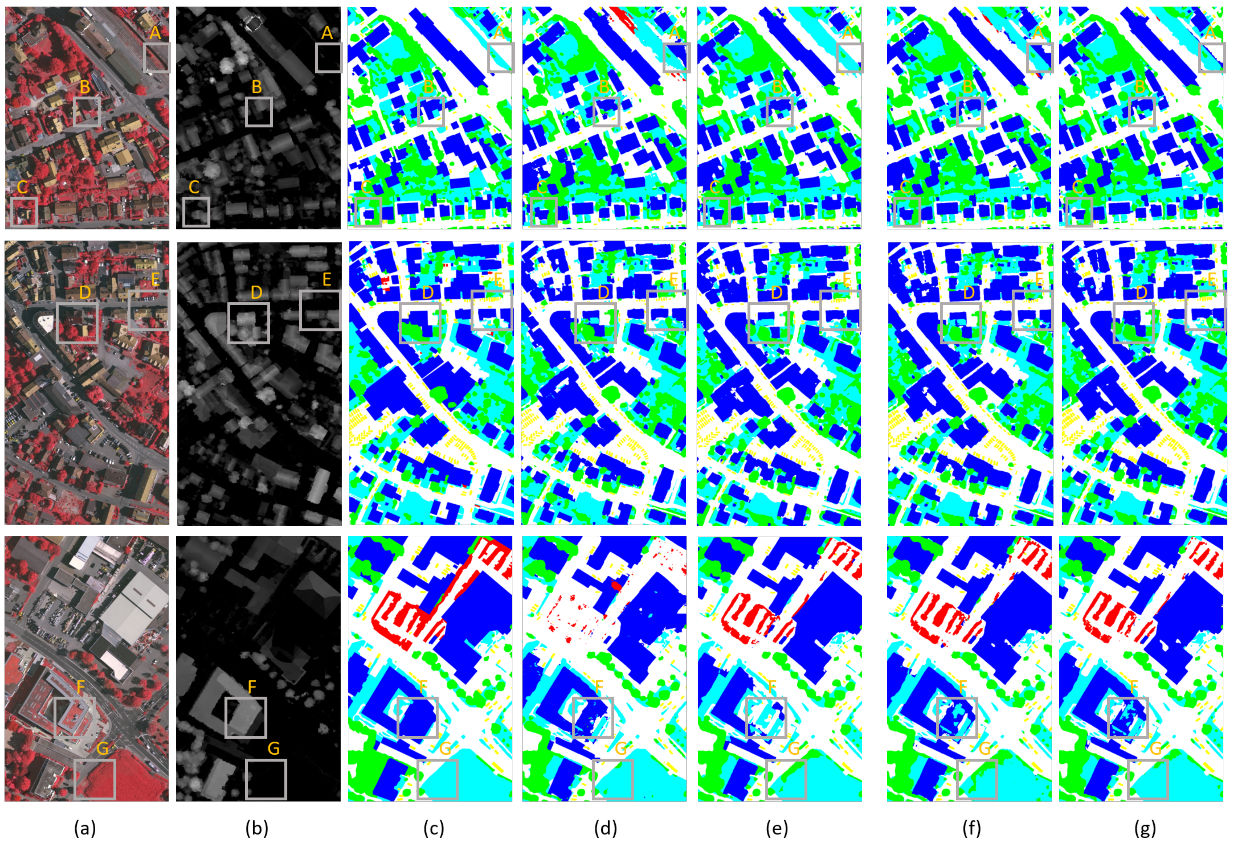
This subsection demonstrates advantages of introducing depth information by comparing visual inference of different methods. Figure 5 shows testing images and full inference maps of three areas from Vaihingen dataset. Figure 6 shows details of seven regions framed in Figure 5.
In depth maps, ground objects with higher elevation have brighter pixels. Introducing depth helps the model to distinguish those pixels that are easy to be confused. Rectangle A (Swin and EDFT classify right) and C (only EDFT classifies right) are examples of impervious surface misclassified to the building, while B (only Segformer classify wrong) is an example of a building misclassified as an impervious surface. The appearance of A and C (For the sake of illustration, we may use the label referring to the problematic part not the whole patch) are very similar to the building, and especially in A there is a bounding wall like the edge of the building. Near the edge of the building in B, some pixels are labeled correctly, but more pixels are classified to impervious surface out of similar appearance. D (only EDFT classifies right) is an example of a building misclassified as low vegetation. Instead, EDFT can label these examples correctly by taking depth into consideration.
In addition to improving the model’s ability to distinguish impervious surface from building, introducing depth helps the model tell apart low vegetation and tree. Obviously, using absolute elevation of ground objects can distinguish low vegetation from tree like G (Upernet and EDFT classify right), but EDFT does not work in this way. The model still classifies those low vegetation pixels on the building correctly in F and B, although ground truth regards them as buildings. There are also some disadvantages of introducing depth. The segmentation accuracy is influenced by the accuracy of depth. As there is a height mistake in E (only EDFT classifies wrong), EDFT misclassifies the road between two houses as a building. To be noticed, there are some other factors not shown in the pictures, such as mistakes of ground truth and boundary flaws of orthophoto.
4.2.4. Confusion Matrices
This subsection displays the visualization results of confusion matrices. Figure 7e,f demonstrate clearly the benefit of introducing depth, and the advantages of EDFT over conventional two-stream network. From the quantitative result, we could also draw the same conclusion as in the previous section.
Introducing depth helps the model to classify those classes that are easy to be confused. It increases the building accuracy by decreasing the number of pixels which are impervious surfaces or low vegetation but were misclassified as buildings. By correct handling those “hard” pixels, the TP vales of four classes all increase. To be noticed, clutter are objects not belong to the five other class and are less important.
EDFT has a stronger ability to distinguish low vegetation from tree than conventional two-stream network. It may be owed to DSA-add, which treats depth in a softer way. As Figure 7e shows, “two-stream-same” is likely to convert some pixels of the low vegetation class to the tree class. However, in Figure 7f, the number of pixels which are trees but are misclassified does not increase too much, and thus, the ability to distinguish the two classes has improved.
4.3. Ablation Study
4.3.1. Downsample Scheme
EDFT differs from a traditional two-stream network in two main points: It only uses downsampling to extract depth features and uses self-attention to fuse features of two modalities. It is necessary to confirm through the experiment which sampling scheme is the most appropriate. The experiments use convolution to downsample images, and discusses whether it is necessary to introduce local information, and whether it is necessary to retain information loss caused by the downsampling operation. The results in Table 4 show that retaining the information lost in the downsampling operation by expanding the dimension of the output feature channel is beneficial to improving the accuracy, while the introduction of local information has its advantages and disadvantages. Simply put, the final EDFT employs overlapped patch merging to conduct downsampling.
4.3.2. Attention Type
To mitigate the gap caused by the difference between two branches and two modalities, we use an attention model fusing two features. Here, we discuss the effect of different attention mechanisms towards multi-modal feature fusion in the case of “two stream-differ”. Two common attention types (SE-Block [21], CBAM [43]) and two proposed self-attentions (DSA-concat, DSA-add) are compared in Figure 8.To be fair, we replace the self-attention module in Figure 2 with the SE-Block(implemented in mmseg) and CBAM (implemented in the official codebase [43]), separately.
Surprisingly, two kinds of channel attention modules (SE-Block, CBAM) lower the accuracy of models for all sizes. The following two reasons could lead to this result: residual connection or slice operation in Figure 2 may not suit to channel attention, channel attention may not work in the case of transformer architecture, or the two branches differ too much.
On the contrary, both of DSA-concat and DSA-add work well. It demonstrates the capability of self-attention mechanism on the problem of multi-modal feature fusion. For the small model (B0-B3), DSA-concat lives up to our expectation and performs better than the baseline “two-stream-differ”. However, for the large model, the DSA-concat module is out of function, and its performance is similar to “two-stream-differ”. We infer that when color and depth come to choices, the DSA-concat module in large model tends to trust the color feature and assigns more weight, as the color branch is deeper and bigger, and thus the color feature is more reliable. The DSA-add module adopts another way to measure and combine depth similarity. Using the weight parameter to force the network to consider depth information, it obtains the best performance over all model sizes.
4.3.3. Weight Parameter
To leverage the potential of the DSA-add module, different weight parameters are tested on the model of each size. As color and depth features are normalized before self-attention, the testing weight parameters range from 0.1 to 2.0, and the interval is set to 0.1. Table 5 shows the best weight setting for each model. In general, the small model prefers a depth attention of small weight.
5. Discussion
Semantic segmentation, as one of the three basic tasks of computer vision, has been greatly improved by the development of deep learning. We can achieve good results by merely using visible images of existing remote sensing datasets, but it is still far from being applied in practical remote sensing engineering. The introduction of ground object elevation information can be treated as a means of auxiliary classification, helping to improve the accuracy of some specific classes, which is preferred in some situations. Despite the fact that with the increasing model size, the inference becomes more accurate and the experimental results approach the upper limit of the segmentation accuracy of the dataset, our model still benefits from introducing elevation information. Moreover, additional information can improve the upper limit of segmentation accuracy, which may be highlighted in the future when a more challenging remote sensing dataset is published.
This paper not only uses elevation information to improve segmentation accuracy but also fuses elevation information by a lightweight way with a few extra computation costs. The minimal model contains only 4.49 million parameters, suitable for carrying on a mobile device and performing real-time segmentation.
The experimental results concerning two kinds of DSA modules show that adopting weight parameters to balance color and depth features achieves higher segmentation accuracy and prevents depth from losing its effect in the case of large models. Although it is not easy to find the best weight, combining attention on different features may be the correct way to exploit multi-modal data (not limited to RGB-D data but also includes multispectral data, even point clouds and images). The best way to measure the similarity of different modalities and the adaptive combination method without weight needs to be studied in the future.
6. Conclusions
Based on the intuition that the original depth map is a feature in itself, this paper improves the traditional two-stream network for RGB-D segmentation from the computational aspect. The major conclusions are the following:
- Depth feature acquired by simple downsampling on the original depth map are also beneficial to segmentation. Identical branches in two-stream network are not necessary;
- Addition fusion ignores the gap between two modalities and two branches. Applying attention in the fusion problem to decide which feature is more reliable achieves better performance;
- Computing attention on multi-modal data by combining similarities can obtain better results than concatenating data in the input phase.
Author Contributions
Conceptualization, J.H. and H.X.; methodology, J.H., L.Y., and H.X.; validation, J.H. and Z.G.; formal analysis, J.H.; writing—original draft preparation, J.H.; writing—review and editing, H.X., P.W., and J.H.; project administration, L.Y.; funding acquisition, L.Y. All authors have read and agreed to the published version of the manuscript.
Funding
This study was supported by National Key Research and Development Project (2020YFD1100200), and the Science and Technology Major Project of Hubei Province (2021AAA010).
Institutional Review Board Statement
Not applicable.
Informed Consent Statement
Not applicable.
Data Availability Statement
No new data were created or analyzed in this study.
Acknowledgments
A publicly available GitHub repository mmseg was adapted for our experiments.
Conflicts of Interest
The authors declare no conflict of interest.
References
- Shelhamer, E.; Long, J.; Darrell, T. Fully Convolutional Networks for Semantic Segmentation. IEEE Trans. Pattern Anal. Mach. Intell. 2017, 39, 640–651. [Google Scholar] [CrossRef] [PubMed]
- He, K.; Zhang, X.; Ren, S.; Sun, J. Deep Residual Learning for Image Recognition. In Proceedings of the IEEE Conference on Computer Vision and Pattern Recognition (CVPR), Las Vegas, NV, USA, 26 June–1 July 2016; pp. 770–778. [Google Scholar]
- Yu, F.; Koltun, V. Multi-Scale Context Aggregation by Dilated Convolutions. In Proceedings of the International Conference on Learning Representations (ICLR), San Juan, Puerto Rico, 2–4 May 2016. [Google Scholar]
- Dosovitskiy, A.; Beyer, L.; Kolesnikov, A.; Weissenborn, D.; Zhai, X.; Unterthiner, T.; Dehghani, M.; Minderer, M.; Heigold, G.; Gelly, S.; et al. An Image is Worth 16 × 16 Words: Transformers for Image Recognition at Scale. In Proceedings of the International Conference on Learning Representations (ICLR), Online, 3–7 May 2021. [Google Scholar]
- Kampffmeyer, M.; Salberg, A.B.; Jenssen, R. Semantic Segmentation of Small Objects and Modeling of Uncertainty in Urban Remote Sensing Images Using Deep Convolutional Neural Networks. In Proceedings of the IEEE Conference on Computer Vision and Pattern Recognition Workshops (CVPRW), Las Vegas, NV, USA, 26 June–1 July 2016; pp. 680–688. [Google Scholar]
- Audebert, N.; Le Saux, B.; Lefèvre, S. Semantic Segmentation of Earth Observation Data Using Multimodal and Multi-scale Deep Networks. In Proceedings of the Asian Conference on Computer Vision (ACCV), Taipei, Taiwan, 20–24 November 2016; pp. 180–196. [Google Scholar]
- Zhang, W.; Huang, H.; Schmitz, M.; Sun, X.; Wang, H.; Mayer, H. Effective Fusion of Multi-Modal Remote Sensing Data in a Fully Convolutional Network for Semantic Labeling. Remote Sens. 2018, 10, 52. [Google Scholar] [CrossRef] [Green Version]
- Audebert, N.; Le Saux, B.; Lefèvre, S. Beyond RGB: Very high resolution urban remote sensing with multimodal deep networks. ISPRS J. Photogramm. Remote Sens. 2018, 140, 20–32. [Google Scholar] [CrossRef] [Green Version]
- Hazirbas, C.; Ma, L.; Domokos, C.; Cremers, D. FuseNet: Incorporating Depth into Semantic Segmentation via Fusion-Based CNN Architecture. In Proceedings of the Asian Conference on Computer Vision (ACCV), Taipei, Taiwan, 20–24 November 2016; pp. 213–228. [Google Scholar]
- Hu, X.; Yang, K.; Fei, L.; Wang, K. ACNET: Attention Based Network to Exploit Complementary Features for RGBD Semantic Segmentation. In Proceedings of the IEEE International Conference on Image Processing (ICIP), Taipei, Taiwan, 22–25 September 2019; pp. 1440–1444. [Google Scholar]
- Chen, X.; Lin, K.Y.; Wang, J.; Wu, W.; Qian, C.; Li, H.; Zeng, G. Bi-directional Cross-Modality Feature Propagation with Separation-and-Aggregation Gate for RGB-D Semantic Segmentation. In Proceedings of the European Conference on Computer Cision (ECCV), Glasgow, UK, 23–28 August 2020; pp. 561–577. [Google Scholar]
- Luo, H.; Chen, C.; Fang, L.; Zhu, X.; Lu, L. High-Resolution Aerial Images Semantic Segmentation Using Deep Fully Convolutional Network With Channel Attention Mechanism. IEEE J. Sel. Top. Appl. Earth Obs. Remote Sens. 2019, 12, 3492–3507. [Google Scholar] [CrossRef]
- Cheng, Y.; Cai, R.; Li, Z.; Zhao, X.; Huang, K. Locality-Sensitive Deconvolution Networks with Gated Fusion for RGB-D Indoor Semantic Segmentation. In Proceedings of the IEEE Conference on Computer Vision and Pattern Recognition (CVPR), Honolulu, HI, USA, 21–26 July 2017; pp. 1475–1483. [Google Scholar]
- Liu, H.; Wu, W.; Wang, X.; Qian, Y. RGB-D joint modelling with scene geometric information for indoor semantic segmentation. Multimed. Tools Appl. 2018, 77, 22475–22488. [Google Scholar] [CrossRef]
- Wang, W.; Ulrich, N. Depth-Aware CNN for RGB-D Segmentation. In Proceedings of the European Conference on Computer Cision (ECCV), Munich, Germany, 8–14 September 2018; pp. 144–161. [Google Scholar]
- Xing, Y.; Wang, J.; Chen, X.; Zeng, G. 2.5D Convolution for RGB-D Semantic Segmentation. In Proceedings of the IEEE International Conference on Image Processing (ICIP), Taipei, Taiwan, 22–25 September 2019; pp. 1410–1414.
- Xing, Y.; Wang, J.; Zeng, G. Malleable 2.5D Convolution: Learning Receptive Fields along the Depth-axis for RGB-D Scene Parsing. In Proceedings of the European Conference on Computer Cision (ECCV), Glasgow, UK, 23–28 August 2020; pp. 555–571. [Google Scholar]
- Chen, R.; Zhang, F.L.; Rhee, T. Edge-Aware Convolution for RGB-D Image Segmentation. In Proceedings of the 35th International Conference on Image and Vision Computing New Zealand (IVCNZ), Wellington, New Zealand, 25–27 November 2020; pp. 1–6. [Google Scholar]
- Liu, Z.; Lin, Y.; Cao, Y.; Hu, H.; Wei, Y.; Zhang, Z.; Lin, S.; Guo, B. Swin Transformer: Hierarchical Vision Transformer using Shifted Windows. In Proceedings of the IEEE International Conference on Computer Vision (ICCV), Online, 11–17 October 2021. [Google Scholar]
- Sun, Y.; Tian, Y.; Xu, Y. Problems of encoder-decoder frameworks for high-resolution remote sensing image segmentation: Structural stereotype and insufficient learning. Neurocomputing 2019, 330, 297–304. [Google Scholar] [CrossRef]
- Hu, J.; Shen, L.; Albanie, S.; Sun, G.; Wu, E. Squeeze-and-Excitation Networks. IEEE Trans. Pattern Anal. Mach. Intell. 2020, 42, 2011–2023. [Google Scholar] [CrossRef] [PubMed] [Green Version]
- Mou, L.; Hua, Y.; Zhu, X.X. A Relation-Augmented Fully Convolutional Network for Semantic Segmentation in Aerial Scenes. In Proceedings of the IEEE Conference on Computer Vision and Pattern Recognition (CVPR), Long Beach, CA, USA, 15–20 June 2019; pp. 12408–12417. [Google Scholar]
- Niu, R.; Sun, X.; Tian, Y.; Diao, W.; Chen, K.; Fu, K. Hybrid Multiple Attention Network for Semantic Segmentation in Aerial Images. IEEE Trans. Geosci. Remote Sens. 2022, 60, 1–18. [Google Scholar] [CrossRef]
- Li, R.; Zheng, S.; Duan, C.; Su, J.; Zhang, C. Multistage Attention ResU-Net for Semantic Segmentation of Fine-Resolution Remote Sensing Images. IEEE Geosci. Remote Sens. Lett. 2022, 19, 1–5. [Google Scholar] [CrossRef]
- Wang, L.; Li, R.; Duan, C.; Zhang, C.; Meng, X.; Fang, S. A Novel Transformer based Semantic Segmentation Scheme for Fine-Resolution Remote Sensing Images. IEEE Geosci. Remote Sens. Lett. 2022, 19. [Google Scholar] [CrossRef]
- Xu, Z.; Zhang, W.; Zhang, T.; Yang, Z.; Li, J. Efficient Transformer for Remote Sensing Image Segmentation. Remote Sens. 2021, 13, 3585. [Google Scholar] [CrossRef]
- Fooladgar, F.; Kasaei, S. A survey on indoor RGB-D semantic segmentation: From hand-crafted features to deep convolutional neural networks. Multimed. Tools Appl. 2020, 79, 4499–4524. [Google Scholar] [CrossRef]
- Chen, K.; Fu, K.; Gao, X.; Yan, M.; Zhang, W.; Zhang, Y.; Sun, X. Effective Fusion of Multi-Modal Data with Group Convolutions for Semantic Segmentation of Aerial Imagery. In Proceedings of the IEEE International Geoscience and Remote Sensing Symposium (IGARSS), Yokohama, Japan, 28 July–2 August 2019; pp. 3911–3914. [Google Scholar]
- Volpi, M.; Tuia, D. Dense Semantic Labeling of Subdecimeter Resolution Images With Convolutional Neural Networks. IEEE Trans. Geosci. Remote Sens. 2017, 55, 881–893. [Google Scholar] [CrossRef] [Green Version]
- Marcos, D.; Volpi, M.; Kellenberger, B.; Tuia, D. Land cover mapping at very high resolution with rotation equivariant CNNs: Towards small yet accurate models. ISPRS J. Photogramm. Remote Sens. 2018, 145, 96–107. [Google Scholar] [CrossRef] [Green Version]
- Maggiori, E.; Tarabalka, Y.; Charpiat, G.; Alliez, P. High-Resolution Aerial Image Labeling With Convolutional Neural Networks. IEEE Trans. Geosci. Remote Sens. 2017, 55, 7092–7103. [Google Scholar] [CrossRef] [Green Version]
- Xie, E.; Wang, W.; Yu, Z.; Anandkumar, A.; Lvarez, J.E.M.A.; Luo, P. SegFormer: Simple and Efficient Design for Semantic Segmentation with Transformers. In Proceedings of the Advances in Neural Information Processing Systems (NIPS), Online, 6–14 December 2021. [Google Scholar]
- Badrinarayanan, V.; Kendall, A.; Cipolla, R. SegNet: A Deep Convolutional Encoder-Decoder Architecture for Image Segmentation. IEEE Trans. Pattern Anal. Mach. Intell. 2017, 39, 2481–2495. [Google Scholar] [CrossRef] [PubMed]
- Ronneberger, O.; Fischer, P.; Brox, T. U-Net: Convolutional Networks for Biomedical Image Segmentation. In Proceedings of the Medical Image Computing and Computer-Assisted Intervention (MICCAI), Munich, Germany, 5–9 October 2015; pp. 234–241. [Google Scholar]
- Zhao, H.; Jia, J.; Koltun, V. Exploring Self-Attention for Image Recognition. In Proceedings of the IEEE Conference on Computer Vision and Pattern Recognition (CVPR), Seattle, WA, USA, 13–19 June 2020; pp. 10073–10082. [Google Scholar]
- Wang, Q.; Wu, B.; Zhu, P.; Li, P.; Zuo, W.; Hu, Q. ECA-Net: Efficient Channel Attention for Deep Convolutional Neural Networks. In Proceedings of the IEEE Conference on Computer Vision and Pattern Recognition (CVPR), Seattle, WA, USA, 13–19 June 2020; pp. 11531–11539. [Google Scholar]
- Marmanis, D.; Schindler, K.; Wegner, J.D.; Galliani, S.; Datcu, M.; Stilla, U. Classification with an edge: Improving semantic image segmentation with boundary detection. ISPRS J. Photogramm. Remote Sens. 2018, 135, 158–172. [Google Scholar] [CrossRef] [Green Version]
- Gerke, M. Use of the Stair Vision Library within the ISPRS 2D Semantic Labeling Benchmark (Vaihingen); ResearcheGate: Berlin, Germany, 2015. [Google Scholar] [CrossRef]
- Yue, K.; Yang, L.; Li, R.; Hu, W.; Zhang, F.; Li, W. TreeUNet: Adaptive Tree convolutional neural networks for subdecimeter aerial image segmentation. ISPRS J. Photogramm. Remote Sens. 2019, 156, 1–13. [Google Scholar] [CrossRef]
- Liu, Y.; Fan, B.; Wang, L.; Bai, J.; Xiang, S.; Pan, C. Semantic labeling in very high resolution images via a self-cascaded convolutional neural network. ISPRS J. Photogramm. Remote Sens. 2018, 145, 78–95. [Google Scholar] [CrossRef] [Green Version]
- Li, X.; Wen, C.; Wang, L.; Fang, Y. Geometry-Aware Segmentation of Remote Sensing Images via Joint Height Estimation. IEEE Geosci. Remote Sens. Lett. 2022, 19, 1–5. [Google Scholar] [CrossRef]
- Xiao, T.; Liu, Y.; Zhou, B.; Jiang, Y.; Sun, J. Unified Perceptual Parsing for Scene Understanding. In Proceedings of the European Conference on Computer Cision (ECCV), Munich, Germany, 8–14 September 2018; pp. 432–448. [Google Scholar]
- Woo, S.; Park, J.; Lee, J.Y.; Kweon, I.S. CBAM: Convolutional Block Attention Module. In Proceedings of the European Conference on Computer Cision (ECCV), Munich, Germany, 8–14 September 2018; pp. 3–19. [Google Scholar]
Figure 1.
Connection between Segformer and our method EDFT. There are three networks depicted in Section 3, differing in the encoder structure. While Segformer only handles color input, the other two networks are designed for RGB-D segmentation.
Figure 1.
Connection between Segformer and our method EDFT. There are three networks depicted in Section 3, differing in the encoder structure. While Segformer only handles color input, the other two networks are designed for RGB-D segmentation.

Figure 2.
Depth-aware Self-attention Module in a concat mode.

Figure 3.
Depth-aware Self-attention Module in an addition mode.

Figure 4.
Performance and model efficiency on Vaihingen test set. For each best configuration, EDFT obtains 0.56% mIoU gains over the baseline method with additional 3.09 millions parameter, while traditional two-stream network (add-same) obtains 0.18% mIoU gains over the baseline method with additional 60.84 millions parameter.

Figure 5.
Visual comparison of different methods: (a) Color images(IRRG); (b) Depth images; (c) Ground truth; (d) Upernet; (e) Swin; (f) Segformer-B4; (g) EDFT-B4. Three rows of images represent the area 10, 27, and 33 from the Vaihingen dataset. The inference map is labeled with impervious surface (white), building (blue), low vegetation (cyan), tree (green), car (yellow), and clutter (red).

Figure 6.
Details of the regions framed in green in Figure 5. From top to bottom, there are seven subfigures labeled from (A–G). The palette and the meaning of each column are the same as above.
Figure 6.
Details of the regions framed in green in Figure 5. From top to bottom, there are seven subfigures labeled from (A–G). The palette and the meaning of each column are the same as above.

Figure 7.
Visualization results of confusion matrices on Vaihingen test set. The top row displays three compared models (Segformer, “two-stream-same”, EDFT), and the model size is B0. The bottom left is the confusion matrix of EDFT without normalization. To make it easier to compare, we visualize the difference between the confusion matrix of Segformer and the one of the other two models (bottom middle and right).

Figure 8.
Effect of attention type on multi-modal feature fusion problem. SE-Block and CBAM don’t work and are even harmful. DSA-add performs best over all model size. DSA-concat is slightly lower than DSA-add on model B0–B3.
Figure 8.
Effect of attention type on multi-modal feature fusion problem. SE-Block and CBAM don’t work and are even harmful. DSA-add performs best over all model size. DSA-concat is slightly lower than DSA-add on model B0–B3.


Table 1.
Comparisons with the state-of-the-art on Vaihingen test set, where * represents the method employing DSM or nDSM, ** represents transformer backbone, and - represents missing data. The values in bold are the best and the values underlined are the second best.
Table 1.
Comparisons with the state-of-the-art on Vaihingen test set, where * represents the method employing DSM or nDSM, ** represents transformer backbone, and - represents missing data. The values in bold are the best and the values underlined are the second best.
| Method | Backbone | Imp.surf. | Building | Low Veg. | Tree | Car | Mean F1 | OA (%) | mIoU (%) |
|---|---|---|---|---|---|---|---|---|---|
| UZ_1 * [29] | CNN-FPL | 89.20 | 92.50 | 81.60 | 86.90 | 57.30 | 81.50 | 87.30 | - |
| Maggiori et al. * [31] | FCN | 91.69 | 95.24 | 79.44 | 88.12 | 78.42 | 86.58 | 88.92 | - |
| S-RA-FCN [22] | VGG-16 | 91.47 | 94.97 | 80.63 | 88.57 | 87.05 | 88.54 | 89.23 | 79.76 |
| V-FuseNet * [8] | VGG-16 | 91.00 | 94.40 | 84.50 | 89.90 | 86.30 | 89.22 | 90.00 | - |
| TreeUNet * [39] | VGG-16 | 92.50 | 94.90 | 83.60 | 89.60 | 85.90 | 89.30 | 90.40 | - |
| VIT [4] | Vit-L ** | 92.7 | 95.32 | 84.36 | 89.73 | 82.28 | 88.88 | 90.67 | 80.33 |
| UperNet [42] | ResNet-101 | 92.37 | 95.62 | 84.44 | 89.97 | 87.92 | 90.06 | 90.71 | 82.14 |
| CASIA [40] | ResNet-101 | 93.20 | 96.00 | 84.70 | 89.90 | 86.70 | 90.10 | 91.10 | - |
| Swin [19] | Swin-S ** | 93.21 | 95.97 | 84.9 | 90.21 | 87.74 | 90.41 | 91.26 | 82.73 |
| GANet * [41] | ResNet-101 | 93.10 | 95.90 | 84.60 | 90.10 | 88.40 | 90.42 | 91.30 | - |
| HUSTW [20] | ResegNet | 93.30 | 96.10 | 86.40 | 90.80 | 74.60 | 88.24 | 91.60 | - |
| HMANet [23] | ResNet-101 | 93.50 | 95.86 | 85.41 | 90.40 | 89.63 | 90.96 | 91.44 | 83.49 |
| Segformer [32] | MiT-B4 ** | 93.49 | 96.27 | 85.09 | 90.31 | 89.63 | 90.96 | 91.51 | 83.63 |
| EDFT (ours) * | MiT-B4 ** | 93.40 | 96.35 | 85.52 | 90.57 | 89.55 | 91.08 | 91.65 | 83.82 |
Table 2.
Comparisons with state-of-the-art on Potsdam test set, where * represents the method employing DSM or NDSM, ** represents transformer backbone, and - represents missing data. The values in bold are the best and the values underlined are the second best.
Table 2.
Comparisons with state-of-the-art on Potsdam test set, where * represents the method employing DSM or NDSM, ** represents transformer backbone, and - represents missing data. The values in bold are the best and the values underlined are the second best.
| Method | Backbone | Imp.surf. | Building | Low Veg. | Tree | Car | Mean F1 | OA (%) | mIoU (%) |
|---|---|---|---|---|---|---|---|---|---|
| UZ_1 * [29] | CNN-FPL | 89.30 | 95.40 | 81.80 | 80.50 | 86.50 | 86.70 | 85.80 | - |
| Maggiori et al. * [31] | FCN | 89.31 | 94.37 | 84.83 | 81.10 | 93.56 | 86.62 | 87.02 | - |
| S-RA-FCN [22] | VGG-16 | 91.33 | 94.70 | 86.81 | 83.47 | 94.52 | 90.17 | 88.59 | 82.38 |
| VIT [4] | Vit-L ** | 93.17 | 95.90 | 87.11 | 88.04 | 94.88 | 91.82 | 90.42 | 85.08 |
| UperNet [42] | Resnet-101 | 93.27 | 96.78 | 86.82 | 88.62 | 96.07 | 92.31 | 90.42 | 85.97 |
| V-FuseNet * [8] | VGG-16 | 92.70 | 96.30 | 87.30 | 88.50 | 95.40 | 92.04 | 90.60 | - |
| TreeUNet * [39] | VGG-16 | 93.10 | 97.30 | 86.60 | 87.10 | 95.80 | 91.98 | 90.70 | - |
| CASIA [40] | ResNet-101 | 93.40 | 96.80 | 87.60 | 88.30 | 96.10 | 92.44 | 91.00 | - |
| GANet * [41] | ResNet-101 | 93.00 | 97.30 | 88.20 | 89.50 | 96.80 | 92.96 | 91.30 | - |
| HUSTW [20] | ResegNet | 93.60 | 97.60 | 88.50 | 88.80 | 94.60 | 92.62 | 91.60 | - |
| Swin [19] | Swin-S ** | 94.02 | 97.24 | 88.39 | 89.08 | 96.32 | 93.01 | 91.70 | 87.15 |
| Segformer [32] | MiT-B4 ** | 94.27 | 97.43 | 88.28 | 89.09 | 96.25 | 93.07 | 91.78 | 87.26 |
| HMANet [23] | ResNet101 | 93.85 | 97.56 | 88.65 | 89.12 | 96.84 | 93.20 | 92.21 | 87.28 |
| EDFT (ours) * | MiT-B4 ** | 94.08 | 97.31 | 88.63 | 89.29 | 96.53 | 93.17 | 91.85 | 87.43 |
Table 3.
Different decoder’s influence on the Potsdam test set. The values in bold are the best.
| Method | Decoder | Imp.surf. | Building | Low Veg. | Tree | Car | Mean F1 | OA (%) | mIoU (%) |
|---|---|---|---|---|---|---|---|---|---|
| Segformer [32] | ALL-MLP | 94.27 | 97.43 | 88.28 | 89.09 | 96.25 | 93.07 | 91.78 | 87.26 |
| Segformer [32] | Uperhead | 94.33 | 97.48 | 88.38 | 89.24 | 96.27 | 93.14 | 91.87 | 87.38 |
| EDFT (ours) | ALL-MLP | 94.08 | 97.31 | 88.63 | 89.29 | 96.53 | 93.17 | 91.85 | 87.43 |
| EDFT (ours) | Uperhead | 94.17 | 97.50 | 88.64 | 89.66 | 96.42 | 93.28 | 91.91 | 87.61 |
Table 4.
Different downsample scheme on Vaihingen test set. Model size is B4. Convolution on the non-overlapped patch has an even kernel size the same as strides, while overlapped patch merging uses odd kernel size convolution with stride half of kernel size. Patch embedding changes the dimension of convolution output from 1 to C (a user parameter, influence of C, is studied in [32]). Here, the method using no embedding just copies output and expands it to the C dimension.
| Overlap | Embedding | mIoU (%) | OA (%) |
|---|---|---|---|
| 82.39 | 91.02 | ||
| 82.47 | 91.12 | ||
| 82.16 | 90.96 | ||
| 82.26 | 91.21 |
Table 5.
Best weight setting of different models on Vaihingen test set.
| Model | Weight | Mean F1 | OA (%) | mIoU (%) |
|---|---|---|---|---|
| B0 | 0.5 | 89.00 | 90.53 | 80.49 |
| B1 | 0.4 | 89.49 | 90.81 | 81.28 |
| B2 | 0.9 | 90.05 | 91.09 | 82.17 |
| B3 | 0.7 | 90.11 | 91.23 | 82.27 |
| B4 | 0.8 | 90.58 | 91.35 | 83.02 |
| B5 | 1.4 | 90.25 | 91.12 | 82.48 |
Publisher’s Note: MDPI stays neutral with regard to jurisdictional claims in published maps and institutional affiliations. |
© 2022 by the authors. Licensee MDPI, Basel, Switzerland. This article is an open access article distributed under the terms and conditions of the Creative Commons Attribution (CC BY) license (https://creativecommons.org/licenses/by/4.0/).
Share and Cite
MDPI and ACS Style
Yan, L.; Huang, J.; Xie, H.; Wei, P.; Gao, Z. Efficient Depth Fusion Transformer for Aerial Image Semantic Segmentation. Remote Sens. 2022, 14, 1294. https://0-doi-org.brum.beds.ac.uk/10.3390/rs14051294
AMA Style
Yan L, Huang J, Xie H, Wei P, Gao Z. Efficient Depth Fusion Transformer for Aerial Image Semantic Segmentation. Remote Sensing. 2022; 14(5):1294. https://0-doi-org.brum.beds.ac.uk/10.3390/rs14051294
Chicago/Turabian StyleYan, Li, Jianming Huang, Hong Xie, Pengcheng Wei, and Zhao Gao. 2022. "Efficient Depth Fusion Transformer for Aerial Image Semantic Segmentation" Remote Sensing 14, no. 5: 1294. https://0-doi-org.brum.beds.ac.uk/10.3390/rs14051294
Note that from the first issue of 2016, this journal uses article numbers instead of page numbers. See further details here.