
Microtopographic Controls on Erosion and Deposition of a Rilled Hillslope in Eastern Tennessee, USA


1
Department of Geography, University of Tennessee, Knoxville, TN 37996, USA
2
Department of Agriculture, Veterinary and Rangeland Sciences, University of Nevada, Reno, NV 89557, USA
3
Department of Geography and Environmental Studies, Texas State University, San Marcos, TX 78666, USA
*
Author to whom correspondence should be addressed.
Remote Sens. 2022, 14(6), 1315; https://0-doi-org.brum.beds.ac.uk/10.3390/rs14061315
Submission received: 27 December 2021
/
Revised: 22 February 2022
/
Accepted: 7 March 2022
/
Published: 9 March 2022
(This article belongs to the Special Issue Spatial-Temporal Monitoring of Environmental and Ecological Processes Using LiDAR)
Abstract
:Topography plays an important role in shaping the patterns of sediment erosion and deposition of different landscapes. Studies have investigated the role of topography at basin scales, whereas little work has been conducted on hillslopes, partially due to the lack of high-resolution topographic data. We monitored detailed topographic changes of a rilled hillslope in the southeastern United States using terrestrial laser scanning and investigated the influences of various microtopographic factors on erosion and deposition. The results suggest that the contributing area is the most important factor for both rill erosion and deposition. Rills with large contributing areas tend to have high erosion and deposition. Slope is positively related to erosion but negatively related to deposition. Roughness, on the other hand, is positively related to deposition but negatively related to erosion. Higher erosion and lower deposition likely occur on north-facing aspects, possibly because of higher soil moisture resulting from less received solar insolation. Similarly, soil moisture is likely higher in areas with higher terrain wetness index values, leading to higher erosion. This work provides important insight into the sediment dynamic and its microtopographic controls on hillslopes.
1. Introduction
Topography plays an important role in water-induced soil erosion and deposition, mainly through its impacts on surface flow pattern, velocity, and erosive power. Topography is also associated with soil properties, such as soil moisture, organic matter, particle size, affecting infiltration, runoff generation, and ponding [1]. Multiple topographic factors, such as slope length, gradient, and curvature, have been incorporated into various soil erosion models, including the Universal Soil Loss Equation (USLE) [2], Revised Universal Soil Loss Equation (RUSLE) [3], and Water Erosion Prediction Project (WEPP) [4]. However, topography has been primarily represented by a single factor in studies related to hillslope/experimental plots without the consideration of spatially varied terrain characteristics [5,6]. This single topography-related factor has been mainly used to emphasize slope length, gradient, or concavity/convexity [2,3,4,5], while topographic variation (e.g., roughness) has been often incorporated into other nontopographic parameters, for example, the cover factor in USLE.
It is generally accepted that topography affects the patterns of erosion and deposition. However, most of the emphasis has been focused on the basin spatial scale [7,8,9], with only a few attempts at plot or hillslope scales [10,11,12,13]. This may be due to a lack of the means to obtain high-resolution topographic data. Most publicly available digital elevation models (DEMs), particularly those obtained by airborne light detection and ranging (LiDAR), are at point densities or pixel resolutions of 50 cm to a few meters, which is not ideal for the study of microtopographic features related to erosion and deposition at plot or hillslope spatial scales.
Recent development of high-resolution remote sensing technologies, including laser scanning sensors (terrestrial and airborne) and structure from motion (SfM), allows for the mapping of microtopographic terrain features and the detection of geomorphic changes at centimeter- to millimeter-length scales [10,11,13,14,15,16,17,18,19,20,21,22]. Subsequently, a wide range of applications of high-resolution point clouds, meshes, and DEMs have been conducted to quantify detailed hillslope processes over the past decade. Vinci et al. [13] found TLS advantageous compared to manual survey when measuring rill length and erosion volume. Eitel et al. [15] examined the impact of surface roughness on concentrated flow processes and rill erosion on two experimental plots based on centimeter (cm)-resolution DEMs from different times. Hancock et al. [16] used a cm-resolution DEM generated using a terrestrial laser scanner (TLS) as the input for landform evolution modeling. In a comparison analysis, Smith and Vericat [18] found that TLS and SfM can produce comparable measurements of roughness at the plot scale. Neugirg et al. [19] found that compared to SfM, TLS can produce higher precision measurements for erosion detection and quantification. Di Stefano et al. [20] used temporal DEMs created by SfM to study the relationship between rill dimensions, volume, and discharge. Llena et al. [21,22] demonstrated that TLS and SfM can capture surface changing rates up to sub-centimeter levels through a five-year continuous survey of two experimental micro-catchments in the Iberian Peninsula from 2013 to 2018.
Although more and more studies have applied TLS- and SfM-derived high-resolution DEMs to quantify the amount and spatial distribution of hillslope erosion and deposition, few studies have investigated microtopographic controls on hillslope processes and whether the relationships derived at such high centimeter or millimeter resolutions are different from empirical relations derived at plot or basin scales. This study aims to identify key topographic factors that can best explain and predict erosion and deposition on hillslopes and explore the relative importance of each factor on the processes. The detailed research questions include (i) What is the spatial pattern of erosion and deposition on a rilled hillslope? (ii) What are the most important microtopographic factors affecting erosion and deposition, respectively? And (iii) How do the topographic factors influence erosion and deposition at the centimeter scale? This work quantifies the importance of various topographic factors on hillslope processes and provides useful guidance for future studies in predicting and simulating sediment dynamics at fine scales.
2. Study Area
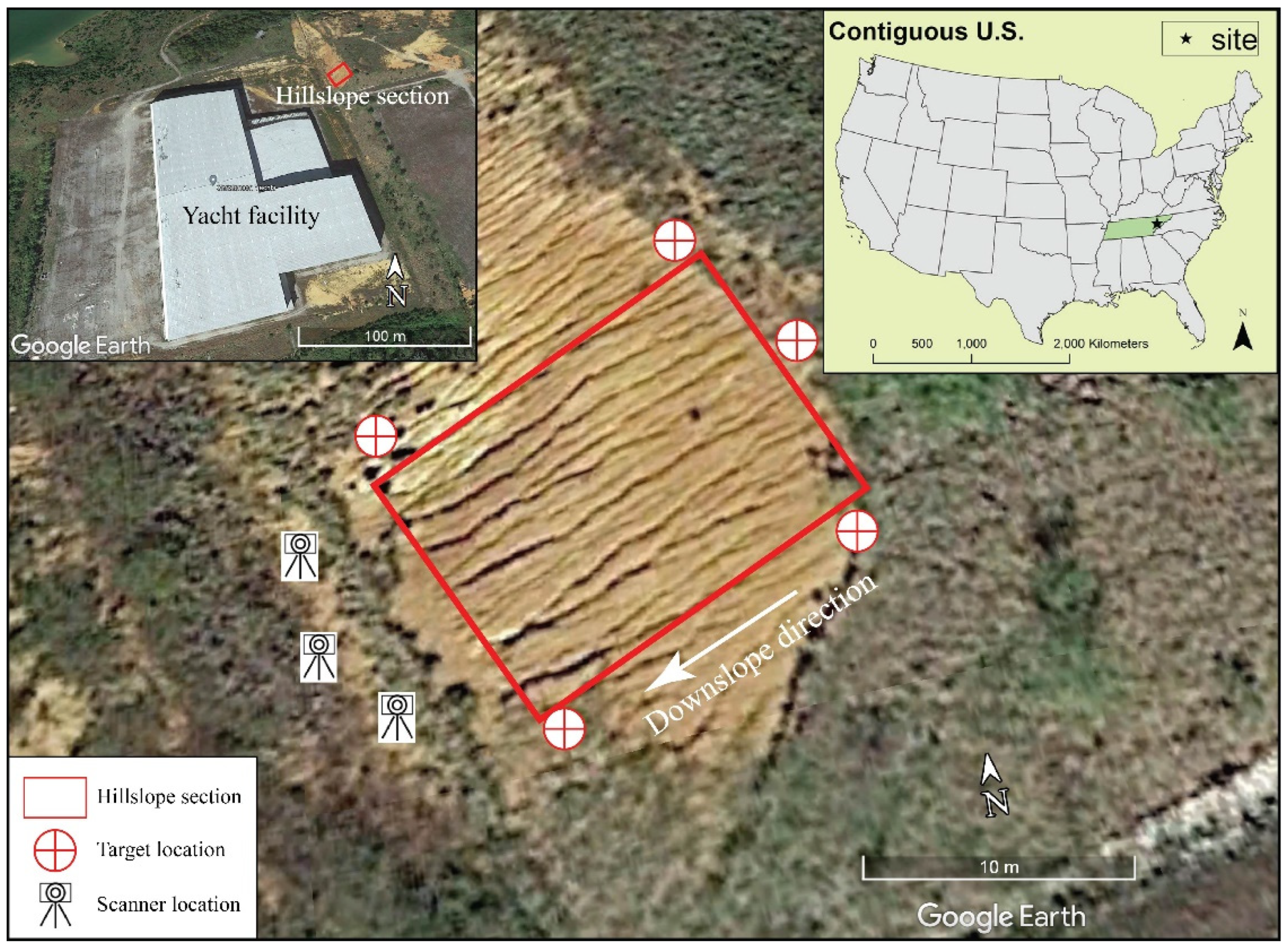
Our study site is located in Loudon County, Tennessee (35°37′32.52′′N, 84°12′59.69′′W, Figure 1). This area is within the Ridge and Valley physiographic province on a terrace of the Little Tennessee River that originates from the Blue Ridge of the southern Appalachian Mountains and meanders westward into the Ridge and Valley. The climate is classified as the Köppen humid subtropical (Cfa) zone that is characterized by perennial precipitation and strong seasonality of hot summers and mild winters. High-intensity precipitation events are frequent due to tropical storms and mid-latitude cyclones. Based on U.S. climate data, the mean annual total precipitation is 1300 mm, and the mean annual temperature is 15 °C in this area (http://www.usclimatedata.com/climate/lenoir-city/tennessee/united-states/ustn0284, accessed on 5 March 2022). The study area is currently dominated by croplands and grassland, with chestnut oak (Quercus prinus) and eastern white pine (Pinus strobus) mixed forests on high elevation ridges and white oak (Quercus alba L.) and tulip poplar (Liriodendron tulipifera) associations in low-elevation valleys.
We monitored the topographic change of a 27° engineered hillslope that was created during the construction of the Christenson Yacht facility in 2007 (Figure 1). The soil of the hillslope is a gradually weathered silt and clayey Ultisols on shale parent material that is susceptible to rilling and gullying [23]. Particle size analyses of six soil samples collected from this site show consistency with the county soil survey with a soil texture of 70.0% clay, 14.7% silt, and 15.3% sand. These edaphic conditions are conducive to intense water erosion, and soil loss in this area has been impairing agricultural productivity and fragmenting the landscapes [24,25].
The hillslope faces southwest at an azimuth of 257° (Figure 1). The altitude of the hillslope ranges from approximately 255 to 263 m above sea level. The hillslope has been almost without vegetation cover and has undergone intensive erosion. Grasses were later planted at the bottom and on the terraces above the hillslope for erosion control. Despite such efforts, rills with lengths up to 20 m have emerged on the hillslope surface from top to toe, detaching and transporting sediment that was subsequently deposited at the base of the hillslope. This study focuses on a vegetation-free section of the hillslope, extending about 18 m in length by 14 m in width. Because no manmade boundaries (earthen berms, metal sheets, etc.) were constructed, the hydrological process is not disturbed in this site, and the erodible materials are not exhaustive, making it ideal for long-term erosion monitoring and observation [26].
3. Materials and Methods
3.1. Data Acquisition
Data acquisitions for this study were previously explained in Lu et al. [10,11]. We conducted five field surveys on 10 December 2014, 7 March 2015, 11 June 2015, 13 September 2015, and 16 December 2015, respectively, using a 1550 nm wavelength FARO Focus3D X 330 TLS with an integrated global positioning system (GPS) and a dual axis compensator to keep data acquisition level and stable. We mounted the scanner on a tripod and set the height of the scanner at approximately 2 m above the ground. This TLS can scan the surrounding areas through a preset or customizable 360° horizontal and 307° vertical view at a nominal ranging radius of 330 m at 90% reflectance. The ranging accuracy of the scanner is ±2 mm at 50 m distance. During each scan, the scanner emits up to 976,000 laser pulses per second. The size of a laser spot is 2.25 mm at sensor exit and the laser beam diverges at 0.19 mrad (0.011°) as it moves further away. In our case, the ranging distance between the scanner and the hillslope surface is approximately 10 to 20 m, corresponding to a laser spot size of 4.15–6.05 mm [27]. We placed five identical spherical reference targets (ATS Scan Reference System with a diameter of 139 mm) around the hillslope before each survey (Figure 1). The targets are important for intra-survey registration, and we distributed them uniformly while avoiding any potential disturbance on the hillslope. We did not install permanent targets because of the concern of theft or vandalism. Because the scan targets are placed slightly differently for each survey, we only used the targets for registering intra-survey scans.
A Trimble GeoExplorer 6000 Series GeoXH™ handheld differential GPS (dGPS) was used to record the locations where the scanner and targets were placed. This dGPS unit has a built-in satellite-based augmentation system to perform the real-time correction on the coordinates once the system locks onto the strongest satellite signal. The nearest GPS base station is at the McGhee Tyson Air National Guard Base (35.81°N, 84.00°W), which is approximately 28 km away from our study site. We performed the dGPS measurement for at least 20 min at each location, allowing for the carrier to update the horizontal accuracy to 10 cm ± 2 parts per million (ppm) and the vertical accuracy to 20 cm ± 2 ppm. Since such level of accuracy is not sufficient for the cm level georeferencing, the coordinates collected by dGPS were only used to coarsely place the scans at their relative locations in the 3D virtual environment before registration. Further details of intra-survey and between-survey registrations are given in Section 3.2.
All TLS surveys were conducted on days with mild temperature and clear sky condition, and at least two days after any precipitation event. Each survey started with a coarse resolution (approximately 5 cm point spacing at 50 m radius) panoramic scan at the maximum viewing angle of the scanner unit (360° horizontal by 307° vertical) about 10 m away from the foot of the hillslope. Three scans were performed subsequently from three different locations at a similar distance from the hillslope. The subsequent scans were parameterized at a much finer resolution (approximately 1 cm spacing at a 50 m distance) to only scan the hillslope. For improved precision and comparable geometry of occlusion we tried to re-occupy the same scanning locations in each survey [28]. However, it was difficult to maintain identical locations due to the continuous change of the environment [29].
3.2. Preprocessing and DEM Generation
A relatively uniform density point cloud can be obtained by registering the point clouds produced by the TLS scans for each survey period (intra-survey registration). The registration was performed in the FARO SCENE® software (version 5.1). This software provides a target-based registration that allows for intra-survey registration between different scans. An iterative closest point algorithm [30] is incorporated in the software to help align the scans on a target-to-target basis. We also visually checked the results of the registration and manually placed different scans using the scan targets and other fixed features, such as the wall of the yacht facility, in each scan to further improve the registration (Table 1).
A panoramic scan was conducted at a relatively coarser resolution to help the registration of the point clouds collected at different survey periods (henceforth called the between-survey registration). The first survey (14 December 2014) was used as the reference point cloud for the four between-survey registrations (Table 1). The root-mean-square error (RMSE) of control points was used to assess the quality of the intra-survey and between-survey registrations (Table 1). The RMSE is calculated in three-dimensional x, y, and z space. The RMSE of the intra-survey registration was calculated based on the offset of the five spherical targets, while the RMSE of the between-survey registration was calculated based on the offset of permanent artificial features (e.g., the walls of the yacht facility) captured in each survey.
Table 1 lists the RMSE values for the intra-survey and between-survey registrations. Approximately 7.7 to 9.0 million points were collected for each survey with the average point density of 1.91–2.25 pts/cm2. The RMSE values range from 0.33 to 0.35 cm for intra-survey registration and from 0.41 to 0.53 cm for between-survey registrations. Both intra- and between-survey RMSE values are comparable to the studies of similar environmental and technological settings [12,13,29,31].
We then rasterized the registered point cloud to produce a DEM for each survey period. No vegetation removal was necessary because this section of the hillslope was free of vegetation. After removing some outlier points, we converted each point cloud to a 1 cm pixel resolution DEM using a bilinear interpolation method in ArcGIS. The 1 cm pixel resolution was determined to best represent sediment estimates based on a previous study [10]. The bilinear interpolation algorithm determines the value of a grid cell using the linear combination of four neighboring cells [32]. It is suitable for continuous surface interpolation without distinct boundaries and has been widely used in converting LiDAR point clouds to raster DEMs [33,34,35].
All five DEMs were output to a local Cartesian projection. This projection focuses on the center point of the area of interest and defines a plane that is tangent to the spheroid at the center point, without accounting for the differences in z between corresponding points on the plane and the spheroid [36]. Note that the distortion in z is negligible due to the small extent of the study area. This projection best preserves the original quality of the data because the scanner stores the points first in polar coordinates that are then converted to Cartesian space.
3.3. DEM of Difference
We used the DEM of difference (DoD) method to calculate the erosion and deposition on the hillslope [37]. The DoD method has been widely used for geomorphic change detection where the differences between two or more DEMs obtained at different times can be quantified based on the following equation [37]:
where t0 is the initial time when the DEM was collected, t1 is the subsequent time of data collection, and ε is the error. The calculation was performed on a cell-to-cell basis to produce a raster with cells of zero, positive, and negative values that spatially represent stable, depositional, and erosional areas on the hillslope, respectively. The error (ε) is related to the ranging error associated with the scanner (±2 mm), the registration errors (Table 1), the noise created by local topographic variation, and the error associated with environmental factors (atmospheric conditions, soil moisture, etc.).
We used the Geometric Change Detection 6.0 (GCD) software with the capability to account for spatially varied uncertainties for the DoD calculation [37]. The GCD uses a fuzzy inference system that applies the fuzzy membership function to assign the uncertainties of each individual cell based on a set of input variables, including point density, roughness, and slope. For example, cells of high point density, low roughness, and low slope gradient are considered with low uncertainty and vice versa. When performing the DoD calculation, the elevation uncertainty is propagated along with uncertainties from various sources (e.g., registration, the survey method), and the elevation change at any cell is only included when the value is significantly (p < 0.05 or 95% confidence level) higher than the propagated uncertainty. A more detailed instruction on the GCD method is available in [37]. We repeated the DoD analysis across the time series, producing four DoD rasters from the five DEMs [10,11]. The elevation changes were only considered at the 95% confidence level. These four DoD rasters allow for the spatial mapping and estimation of both the volume and mass of erosion and deposition within this section of the hillslope [10,11].
3.4. Microtopographic Factors
Hillslope erosion and deposition may be affected by various microtopographic factors. We examined nine factors that are derived from DEMs [38]: elevation, slope, aspect, roughness index (RI), contributing or catchment area (CA), rill density (RD), channel depth (CD), topographic wetness index (TWI), and length-slope factor (LS). These topographic factors were selected because of their impacts on various perspectives of erosion and deposition processes [39,40,41,42,43,44,45,46,47,48,49,50,51,52,53,54,55,56,57] and because they can be derived from DEMs using available GIS software packages, such as ArcGIS [58] and the System for Automated Geoscientific Analyses (SAGA) GIS tools [59].
Elevation is the altitude of a DEM cell, slope is the gradient, and aspect is the azimuth of the slope. Since aspect is a directional variable ranging from 0° to 360°, we transformed it to cosine (CosA) and sine (SinA) values for the analyses.
The roughness index (RI) describes topographic variation and irregularities in the elevation or standardized height of surface features for individual pixels. It is defined as
where x00 is the elevation of the central cell, and xij is the elevation of each neighboring cell in a 3 × 3 window. A high roughness surface reduces erosion by increasing hydraulic resistance, dissipating the flow energy [39,40], and reducing runoff generation [41,42].
Contributing area (CA) is the upstream watershed area of a specific location on the hillslope. CA can be derived using flow direction, flow accumulation, and watershed analysis tools in ArcGIS. It has been widely used for channel network analysis [43,44] and soil erosion prediction [44].
Rill density (RD) is defined as the total length of rills per unit area [45]. It varies for slope steepness, slope length, runoff, soil, and precipitation conditions [46,47]. Channel depth (CD) measures the elevation difference between a specific cell location and its closest drainage divide (watershed boundary). Low CD values represent interfluve areas, while high values represent rill channels. This index has been used in soil classification and geomorphic feature analyses [48,49].
Topographic wetness index (TWI) was proposed to quantify the topographic control on hydrological processes [50]. TWI is defined as
where CA is the contributing area, and θ is the slope angle in degrees. TWI is related to soil depth, infiltration rate, runoff generation, soil texture, and soil aggregates [51,52,53,54,55].
Slope length-gradient (LS) factor is a topographic index used in USLE and RUSLE for soil erosion prediction [2,3,7,56,57]. We derive the LS factor based on the method proposed in [7]:
where is the contributing area at the inlet of grid cell (i,j); D is the cell size; and Gx and Gy represent gradient on x and y directions. The coefficient m is the length exponent of the USLE LS factor, representing the ratio of rill and interrill erosion. It is calculated by the β-value [57]:
The β-value ranges between 0 (the ratio of rill to interrill erosion close to 0) and 1 and is defined as follows [57]:
where θ is the slope angle.
We derived the above nine topographic factors using ArcGIS 10 and SAGA GIS tools for the four 1 cm DEMs (December 2014, March 2015, June 2015, and September 2015). Each of the four DEMs was considered as the initial stages to which the DEM produced in the immediately subsequent survey was compared. The topographic changes occurred between each survey and the next are produced using the DoD method described in Section 3.3.
We used the “sub-watershed” method described in [11] to derive summary statistics (median, sum, or percentage value) for each factor, as well as the erosion and deposition amounts along the rills. The rill network was derived using the hydrology tools in TauDEM [58]. A rill basin refers to all upstream pixels contributing to the lowest outlet point along a rill channel. We generated a set of outlet points at a 0.05 m interval along the rills to segment a rill basin into a series of non-overlapping polygons (sub-watersheds). Although the generated sub-watersheds have various shapes and sizes, a fixed interval guarantees a uniform sampling distance along the rill basin. Please check the reference [11] for detailed description of the “sub-watershed” method.
3.5. Correlation and Regression Analysis
Pearson’s correlation analysis was used to examine the relationships among erosion, deposition, and topographic factors. This analysis produces a correlation coefficient (r) to measure the strength and a p-value to represent the statistical significance of the correlation between each pair of two variables.
We used the linear regression models to examine the relationship between erosion/deposition and topographic factors. The linear models were chosen because they provide clarity and interpretability compared to machine learning models, although they may compromise some predictability. A linear regression model can be expressed as follows:
where y is the dependent variable; x1, x2, …, xn are the independent variables; are the regression coefficients; and is the error.
Both ordinary least squares (OLS) and quantile regression (QR) were used in the analysis. OLS estimates the conditional mean of the dependent variable based on the estimation of regression coefficients () using the minimum of the sum of squared residuals:
OLS is usually used when both dependent and independent variables are normally distributed, and it is not very robust against datasets that have potential outliers.
QR is a modification of OLS that estimates the regression coefficient using the conditional quantile [60]:
where τ is the τth quantile (0 < τ < 1) that is defined as
which satisfies
QR is more robust against the datasets with potential outliers and provides better performance when variables have a non-Gaussian distribution. QR is also ideal when the distribution of the data is skewed, especially when the variables do not exhibit homoscedasticity (similar variance for all independent variables) [60].
Spatial autocorrelation may exist among these topographic factors, violating the assumption of independence for common statistical practices [61]. In our case, various sources might contribute to the spatial autocorrelation of the topographic factors, for example, through hydrological and geomorphic processes associated with erosion and deposition on the hillslope. We used a group k-fold cross-validation method to minimize the influence of spatial autocorrelation while achieving the optimal quantile τ without overfitting. The group k-fold cross-validation method divides data into k groups based on a categorical variable; the cross-validation is repeated for k times, and for each iteration, k-1 groups are used to train the model and the one group that is left out is used to validate the model. The k results from the iterations are eventually averaged to yield an estimation. In this study, a set of parallel rills that were developing on the hillslope comprised our cross-validation dataset. To reduce spatial autocorrelation, we divided the entire dataset into different rill basins based on the rill drainage points close to the foot of the hillslope. We then ensured that the segments within the same rill basin cannot be included in both the training and testing sets.
Since we included various topographic factors that may or may not share redundant information, it is possible for our model to produce biased estimation unless variables are selected in an objective fashion. We used the recursive feature elimination (RFE) with external validation to select the fewest possible variables that preserve the best predictive ability [62]. Sometimes, a backward feature selection approach is used for statistical models: the model loads all variables at the beginning and the least important variable is dropped at each iteration until the model performance converges at an optimal set of variables. However, such an approach is susceptible to overfitting of the training dataset [63]. The RFE approach accounts for such issues by enclosing the backward feature selection within a resampling procedure. For each iteration, the data are partitioned into different training and testing subsets, and the performance of the model is evaluated using the mean squared error (MSE) of the testing subset. The variables included in the final model are determined based on a consensus ranking from all iterations [62].
4. Results
4.1. DEM of Difference
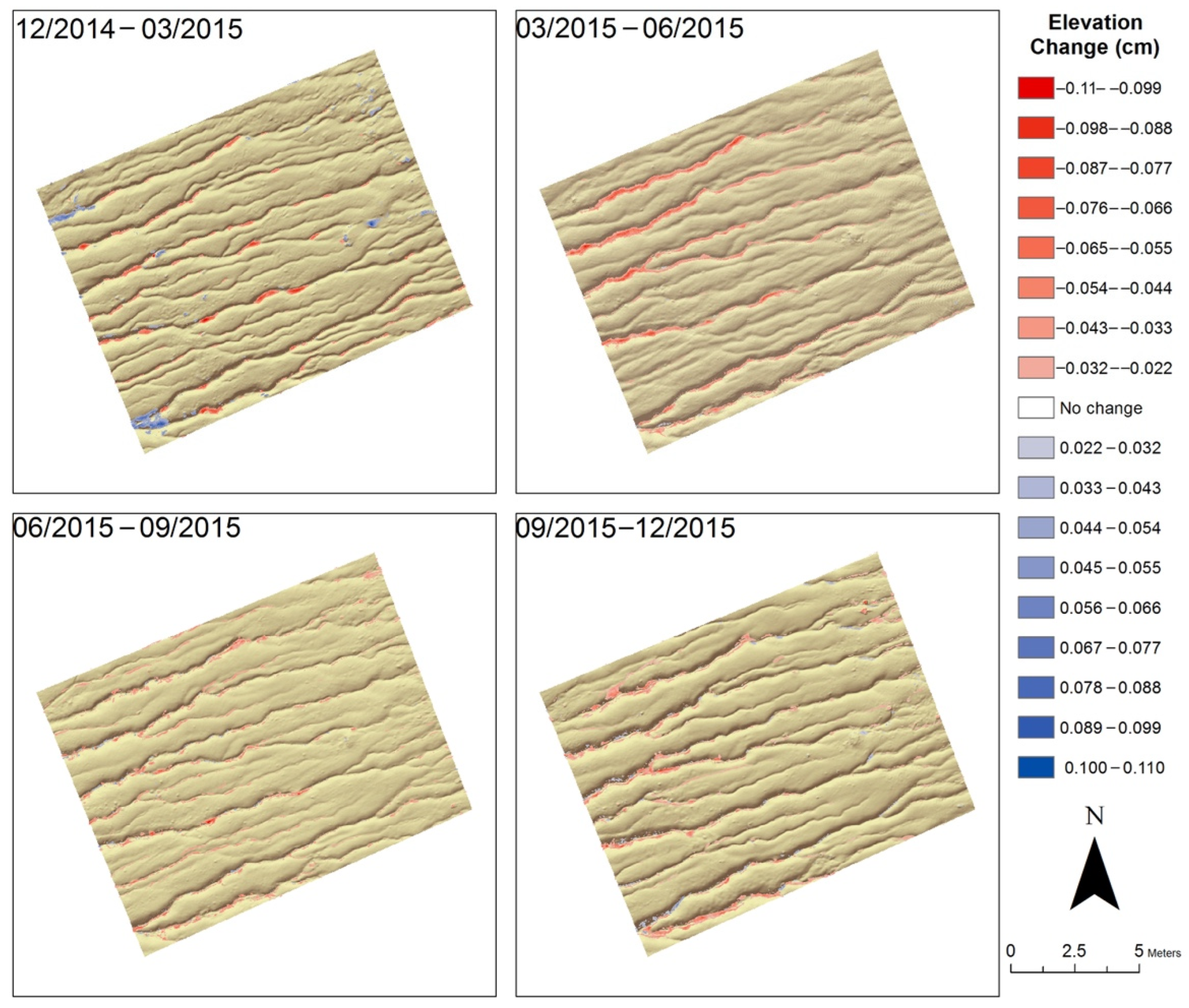
Table 2 summarizes the areal and volumetric changes on the hillslope section during the four periods in 2014–2015. Both erosion and deposition were observed at each period. Overall, this hillslope section underwent intensive erosion with a total of 1.19 ± 0.46 m3 sediment eroded and 0.17 ± 0.08 m3 sediment deposited from December 2014 to December 2015. The net volume change is 1.02 ± 0.54 m3. The March–June period witnessed the largest volume of erosion (0.38 ± 0.16 m3) followed by the September–December period (0.36 ± 0.13 m3). The December 2014–March 2015 and the September–December periods underwent the largest volume of deposition (0.05 ± 0.03 m3 and 0.05 ± 0.02 m3, separately).
Figure 2 illustrates the spatial pattern of erosion and deposition on this hillslope section during the four periods. Generally, the rills are more dynamic compared to interrill areas, with the majority of the detectable changes occurring either within or in proximity to the rills. The majority of the interrill areas are relatively stable with only a few detectable “hotspots” of erosion or deposition.
4.2. Correlation and Regression Analyses
Table 3 shows the results of Pearson’s correlations between the dependent variables and independent variables. Both erosion and deposition are correlated with several independent variables, and many independent variables are correlated with one another. High correlations are observed between some of the variables. For example, the correlation coefficient between slope and the LS factor is 0.83, and the correlation between slope and RI is 0.97. The LS factor is highly correlated with CA (0.73) and RI (0.84). The correlations among independent variables might lead to biased estimation of coefficients and affect the efficacy of the linear regression models.
We used RFE to select the fewest variables that could achieve the minimal MSE. Table 4 shows the results of the RFE. The erosion model and the deposition model achieved the least MSEs with eight and nine variables, respectively. The variables in Table 4 are ranked in correspondence to their importance to the model. In the erosion model, CA is the most important variable. The model with only CA as the independent variable has a relatively high MSE of 0.286. With more variables included in the model, the MSE gradually decreases until it increases again. The second most important factor is slope, followed by CosA, CD, RI, TWI, LS, and elevation. For the deposition model, CA is also of the highest importance, followed by elevation, CD, CosA, TWI, LS, slope, RD, and RI.
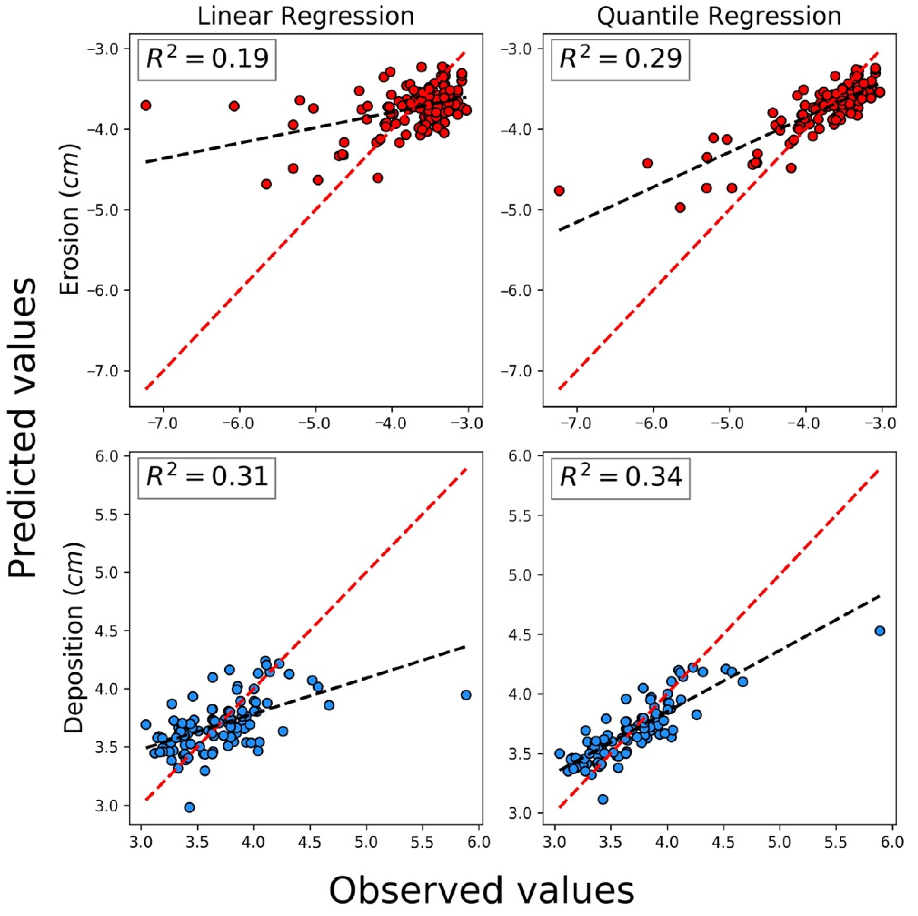
Figure 3 shows the comparison between the observed and predicted erosion/deposition using OLS and QR models. The OLS models produced R2 values of 0.19 and 0.31 for erosion and deposition, respectively. The QR models produce R2 values of 0.29 and 0.34, respectively. The QR models have stronger explanatory capability compared to the OLS models, possibly because the amounts of erosion and deposition do not follow a normal distribution on the hillslope. The QR models also produced less-biased prediction at the extreme values when the optimal quantile parameter was adopted. The predictions made by the QR models showed a better agreement with the observed values compared to those of the OLS models (the black and red dashed lines are closer in QR models).
Table 5, Table 6, Table 7 and Table 8 list the coefficients of RFE-selected topographic variables in the QR models for erosion and deposition during the four scanned periods, respectively, with the quantile (τ) that produces the smallest cross-validation MSE. Generally, CA is associated with higher erosion and deposition, although its coefficient (absolute value) is relatively higher in the erosion model, except for the period from June to September. A steeper slope is associated with higher erosion and lower deposition. In our study area, the hillslope has been incised with well-developed rills, and rill sidewalls are steeper than the interrill and rill floor areas. During rainfall events, erosion would be more significant on rill sidewalls than interrill and rill floor areas. The coefficient of slope, representing the impact of slope on the magnitude of erosion/deposition, is the highest during the period of March to June. This is likely because the soil surface is relatively loose at the beginning of this period after the winter freeze–thaw cycles so that the hillslope is more vulnerable to erosion. Similar to slope, a higher roughness is associated with higher deposition and lower erosion because rugged terrain surface tends to dissipate flow power, reducing transport capacity. Higher elevation leads to lower erosion and lower deposition, which is consistent with the field observation that the areas closer to the top of the hillslope are generally more inactive compared to the foot area. Higher CD values lead to less erosion and more deposition. On this hillslope, areas of high CD values are usually where rills are most deeply incised, such as rill floors; the deeper the rills grow, the more compact and less erodible materials (close to the bedrock) are.
Several other topographic factors affect erosion and deposition through their associations with soil moisture content. Our results suggest that a larger CosA leads to higher erosion and lower deposition. CosA represents the aspect facing a north–south direction, and a larger CosA is closer to north. North-facing areas are more likely have higher soil moisture content in the Northern Hemisphere. These areas are easily saturated, leading to the generation of more runoff during a rainfall event. Similarly, the areas with higher TWI values have higher erosion and lower deposition because TWI estimates the likelihood of water accumulation in an area with elevation differences [51].
5. Discussion
5.1. Seasonal Variation of Erosion and Deposition
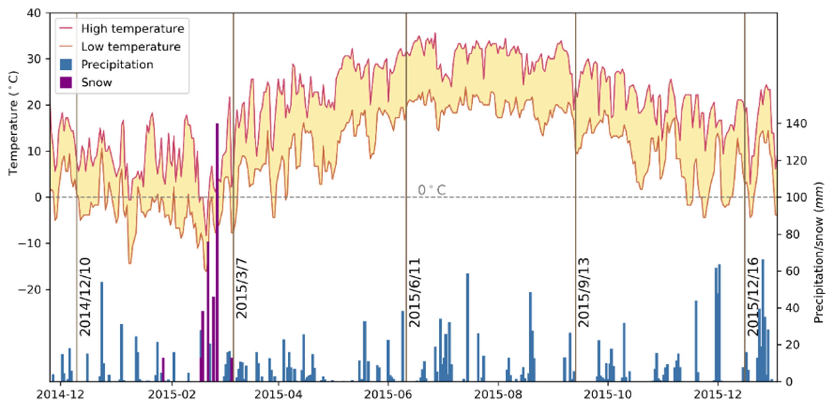
The patterns of erosion and deposition are related to the different precipitation and temperature conditions during the four scan periods. Less erosion and more deposition occurred from December 2014 to March 2015 compared to other periods. This is likely caused by the relatively limited transport capacity during this period. Most days of this period had temperatures below 0 °C at this site, and the observed topographic change might be driven by the freeze–thaw process. Figure 4 illustrates the changes in daily high temperature, low temperature, precipitation, and snow at Lenoir City, TN, USA (35.79°N, 84.26°W, www.usclimatedata.com, accessed on 5 March 2022), approximately 18 km from the study site. The daily low temperature dropped below 0 °C starting late October and fluctuated above and below 0 °C for most days of November, December, and January. Meanwhile, precipitation events may keep the soil moist, allowing for freeze–thaw cycles with the diurnal variation of the temperature. Barnes et al. [64] found that a thin soil layer on the surface can be heaved by ice crystals formed during freezing seasons, and these crystals lead to failures and within-channel deposition during thawing. The mass failures along the sidewalls created by freeze–thaw cycles may widen cross-sections, reducing flow velocities within the rills [65]. The DoD result during the first period suggests that limited transport capacity created more in-channel deposition in the first period, leading to excessive sediment supply in the subsequent period (March to June 2015), shown as the high erosion rate.
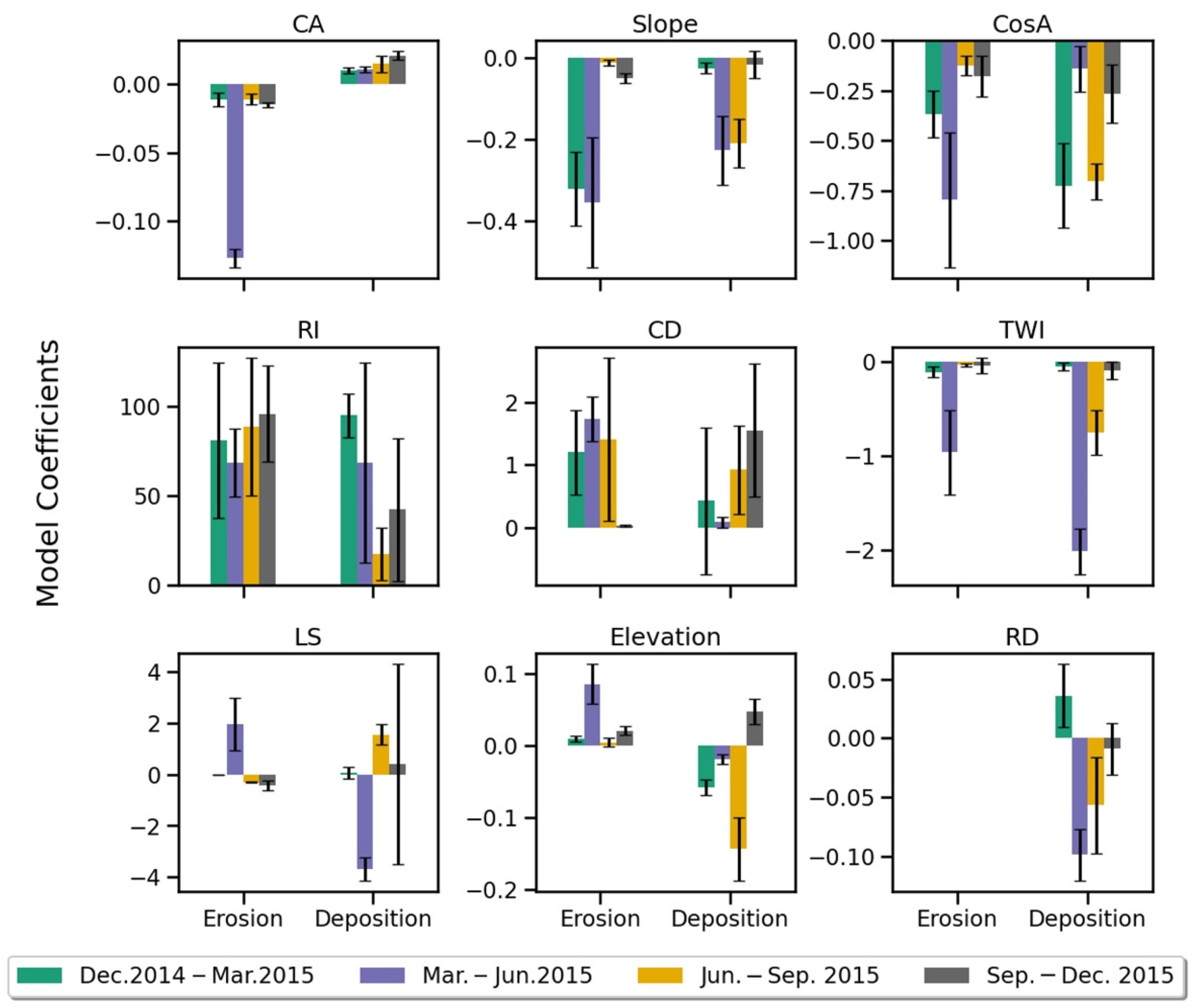
As listed in Table 5, Table 6, Table 7 and Table 8 and shown in Figure 5, the coefficients of the same topographic factor are different in the four survey periods. Note that negative coefficients represent positive influences, while positive coefficients represent negative influences for the topographic factors in the erosion models because erosion values are represented by negative elevation changes. The erosion models show that CA, slope, CosA, and TWI have the highest positive influences, whereas CD, LS, and elevation show the highest negative influences during the March–June period in these four periods. The highest positive or negative influences of these factors during the March–June period are likely associated with the excessive sediment supply following the winter period. Because of the excessive sediment supply, all factors related to surface flow (CA, LS, elevation, and slope), soil moisture (TWI and CosA), and erodibility (CD) actively act on sediment erosion and transportation during the March–June period. In contrast, the decreasing influences of these factors in the following periods likely reflect the limited sediment supply on hillslope after eroding and transporting the excessive sediments during the March–June period. In addition to the spring period (March–June 2015), our results also indicate that slope has a higher influence during the winter (December 2014–March 2015) period than the other two periods. This might suggest that slope, at the microtopographic scale, is strongly associated with erosion during freeze–thaw cycles as well.
For the deposition models, CA has the greatest influence during the September–December 2015 period and the least influence during the December 2014–March 2015 period. CosA and TWI are both negatively related to deposition in all deposition models, with the highest negative influences in the March–June 2015 period. These two factors are associated with soil moisture, and sediments are more erodible or transportable in higher soil moisture areas when sediment supply is excessive, consistent with the results that these two factors have the highest impacts on the erosion models during the same period. Slope had higher negative impacts during March–June 2015 (−0.227) and June–September 2015 (−0.210) periods, suggesting that the areas of higher slope gradients (usually rill headwalls and sidewalls) have less chance of deposition. RI, associated with the flow friction imposed by surface variation, has the highest influence on deposition during the winter period (December 2014–March 2015). This is likely caused by the freeze–thaw cycles, which create more surface irregularity and friction to surface flow, leading to more sediment deposition.
5.2. Factors Controlling Erosion and Deposition
Microtopographic factors show varied importance regarding their impact on erosion and deposition at different scales. CA is the most important variable in all models; both high erosion and deposition occur on the areas with high CA values, reflecting the influence of relative location on the hillslope and within a rill basin. High erosion and low deposition occur on the areas with larger TWI values and on north-facing aspects (larger CosA). Both TWI and aspect are related to soil moisture content, which is likely lower on the areas with lower TWI or CosA (south-facing) values. During a rainfall event, relatively dry soil can absorb more rainfall, postponing and reducing runoff generation. CD is another important factor in most models. CD represents the relative location along the rill cross-sectional profile. A larger CD value suggests low erosion and high deposition in the models. This is because rills have been well developed on the hillslope, and rill floors (high CD areas) have reached a compact layer where the parent materials are not fully decomposed. This compact layer is less erodible than the topsoil of the hillslope. On the other hand, sediments eroded from steep rill sidewalls are likely deposited, at least temporarily, on rill floors where CD is relatively high.
5.3. Limitations of This Work
The complex nature of the erosion and deposition processes introduces challenges to quantifying sediment dynamics at a hillslope scale using grid-based approaches [31,66,67]. The choice of surveying hardware, software, and data processing and analytical methods should be in correspondence with the size of the study area, the features to be monitored, the acceptable level of error, and other factors, such as the frequency of data acquisition and logistic availabilities [10]. TLS is useful in our study by allowing for rapid survey of the hillslope surface without direct interference of the erosional and depositional processes, and the obtained high-resolution topographic data enable the differentiation and quantification of the spatially varied erosion and deposition. However, limited by the uncertainty from various sources, it is still difficult to detect the microtopographic changes on interrill areas.
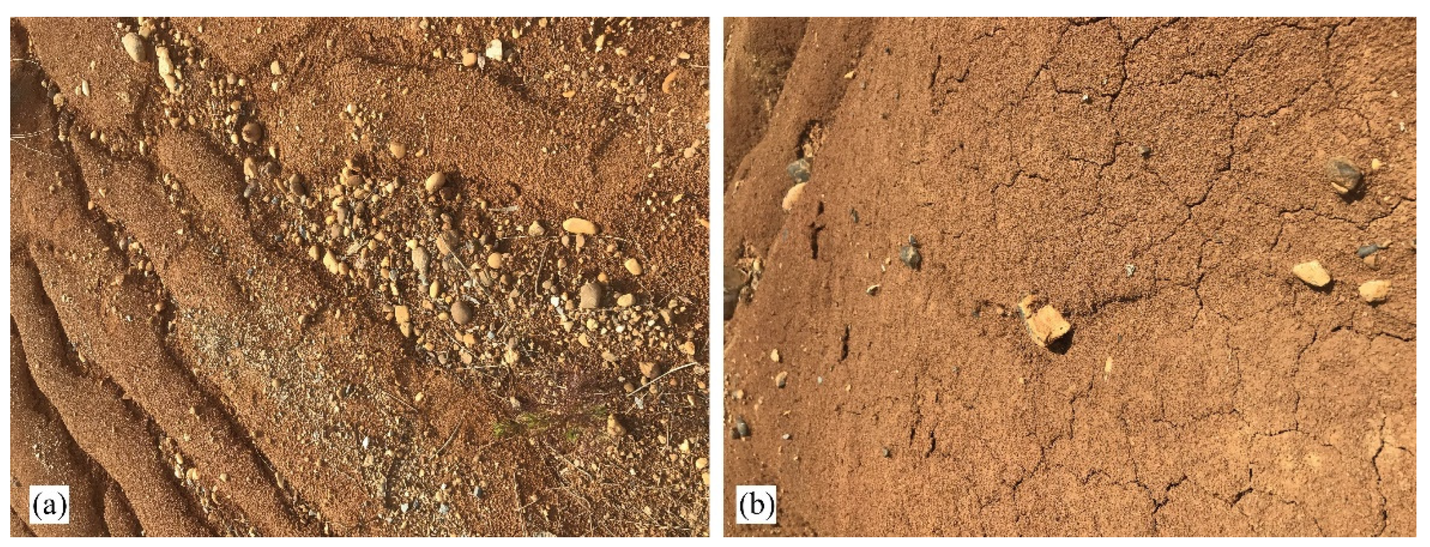
A closer field examination shows that the redistribution of sediment in our study area is further complicated by other factors, including surface armoring and crusting (Figure 6). The erosive power gradually exhausts relatively finer particles (e.g., clay, silt, and fine sand), leaving behind coarser materials, such as some pebbles (Figure 6a). Although our model considered factors such as roughness and TWI as proxies of soil properties, including particle size, organic matter, and soil moisture, these factors are only approximations of the ground truth at best. In situ measurements are impossible as mass sampling at such fine resolution can be expensive, time-consuming, and would inevitably disturb the sediment on the hillslope.
Other factors, such as the pebbles commonly observed on the rill floor, also likely affect the erosion/deposition patterns by altering surface hydrology. The pebbles help prevent raindrop splash and sheet erosion on interrill areas by reducing raindrop impact and dissipating flow energy; they also protect rill floors from further entrenchment. The increase in roughness because of the pebbles reduces the transport capacity, leading to deposition in the rills. We also observed surface crusting on the hillslope (Figure 6b), which can affect raindrop impact on interrill areas [68]. The sporadic crusting may create variation in erodibility between different interrill areas. It is also possible that microorganisms (worms) or animals may disturb the site between surveys, causing potential errors. In addition, the erosion and deposition processes are also affected by rainfall characteristics, such as intensity and duration. More work is needed in the future to examine the impacts of rainfall characteristics on hillslope erosion and deposition.
6. Conclusions
This study examined the influences of microtopographic factors on sediment dynamics on a rilled hillslope in eastern Tennessee, USA, based on linear regression models. Generally, the QR model showed a stronger predictive ability compared to the OLS model, with 29% of the variability for erosion and 34% for deposition explained by the microtopographic variables. The coefficients of nine factors (contributing area, roughness, slope length, gradient, rill density, aspect, TWI, LS factor, and channel depth) reflect the level of their influences on the prediction of erosion or deposition in the QR models. A larger CA leads to higher erosion and deposition. A steeper slope increases erosion and reduces deposition. Roughness is positively related to deposition and negatively related to erosion. Rill floors with larger depth values tend to have less erosion and more deposition. The cosine component of the aspect is associated with higher erosion and lower deposition, possibly due to higher soil moisture on the north-facing aspects with lower solar insolation received. TWI, another index positively associated with soil moisture, is positively related to erosion, and negatively related to deposition. The influences of each topographic factor on erosion and deposition vary in the four periods. The highest positive or negative influences of most topographic factors on erosion during spring are likely associated with the excessive sediment supply accumulated in winter. Then, after eroding and transporting the excessive sediments in spring, the influences of these factors decrease in the following summer and fall periods. The influences of these topographic factors on deposition are mostly consistent with (opposite to) the influences on erosion.
Author Contributions
Conceptualization, Y.L. (Yingkui Li), R.A.W.-A. and X.L.; methodology, X.L., Y.L. (Yingkui Li) and R.A.W.-A.; data collection, processing, and analysis, X.L. and Y.L. (Yingkui Li); writing—original draft preparation, X.L.; writing—review and editing, Y.L. (Yingkui Li), Y.L. (Yanan Li) and R.A.W.-A.; project administration and funding acquisition, X.L. and Y.L. (Yingkui Li). All authors have read and agreed to the published version of the manuscript.
Funding
X.L. received research financial support from the Geomorphology Specialty Group of the American Association of Geographers, the Stewart K. McCroskey Memorial Fund, and the Thomas Fellowship. R.A.W.-A. received startup funding support from the Office of the Vice President for Research & Innovation of the University of Nevada, Reno and a NSF/GLD RAPID EAR-2141804 grant. Funding for open access to this research was provided by the University of Tennessee’s Open Publishing Support Fund.
Institutional Review Board Statement
Not applicable.
Informed Consent Statement
Not applicable.
Data Availability Statement
The data related to this study are available on request from the authors.
Acknowledgments
The authors thank John “Jack” McNelis, Rebecca Potter, Gene Bailey, Martin Walker, Robert Friedrichs, Joseph Robinson, and Yasin Wahid Rabby for the help in the field surveys and Jon Harbor, Daniel Yoder, and Nicholas Nagle for the comments and suggestions in preparation of this manuscript. We also thank four anonymous reviewers for their constructive comments and suggestions to greatly improve this manuscript.
Conflicts of Interest
The authors declare no conflict of interest.
References
- Schneiderman, E.M.; Steenhuis, T.S.; Thongs, D.J.; Easton, Z.M.; Zion, M.S.; Neal, A.L.; Mendoza, G.F.; Todd, W.M. Incorporating variable source area hydrology into a curve-number-based watershed model. Hydrol. Process. 2007, 21, 3420–3430. [Google Scholar] [CrossRef]
- Wischmeier, W.H.; Smith, D.D. Predicting Rainfall Erosion Losses-A Guide to Conservation Planning; United States Department of Agriculture: Hyattsville, MA, USA, 1978. [Google Scholar]
- Renard, K.G.; Foster, G.R.; Weesies, G.; McCool, D.; Yoder, D. Predicting Soil Erosion by Water: A Guide to Conservation Planning with the Revised Universal Soil Loss Equation (RUSLE); US Department of Agriculture: Washington, DC, USA, 1997. [Google Scholar]
- Nearing, M.; Foster, G.; Lane, L.; Finkner, S. A process-based soil erosion model for USDA-Water Erosion Prediction Project technology. Trans. ASAE 1989, 32, 1587–1593. [Google Scholar] [CrossRef]
- Liu, B.; Nearing, M.; Shi, P.; Jia, Z. Slope length effects on soil loss for steep slopes. Soil. Sci. Soc. Am. J. 2000, 64, 1759–1763. [Google Scholar] [CrossRef] [Green Version]
- McCool, D.; Foster, G.; Weesies, G. Slope length and steepness factor (LS). In Predicting Soil Erosion by Water–A Guide to Conservation Planning with Revised Universal Soil Loss Equation (RUSLE); Renard, K.G., Foster, G.R., Weesies, G., McCool, D., Yoder, D., Eds.; USDA: Washington, DC, USA, 1997; Chapter 4; pp. 101–142. [Google Scholar]
- Desmet, P.; Govers, G. A GIS procedure for automatically calculating the USLE LS factor on topographically complex landscape units. J. Soil Water Conserv. 1996, 51, 427–433. [Google Scholar]
- Montgomery, D.R.; Brandon, M.T. Topographic controls on erosion rates in tectonically active mountain ranges. Earth Planet. Sci. Lett. 2002, 201, 481–489. [Google Scholar] [CrossRef]
- Tarolli, P.; Sofia, G.; Dalla, F.G. Geomorphic features extraction from high-resolution topography: Landslide crowns and bank erosion. Nat. Hazards 2012, 61, 65–83. [Google Scholar] [CrossRef]
- Lu, X.; Li, Y.; Washington-Allen, R.A.; Li, Y.; Li, H.; Hu, Q. The effect of grid size on the quantification of erosion, deposition, and rill network. Int. Soil Water Cons. Res. 2017, 5, 241–251. [Google Scholar] [CrossRef]
- Lu, X.; Li, Y.; Washington-Allen, R.A.; Li, Y. Structural and sedimentological connectivity on a rilled hillslope. Sci. Total Environ. 2019, 655, 1479–1494. [Google Scholar] [CrossRef]
- Eltner, A.; Baumgart, P.; Maas, H.G.; Faust, D. Multi-temporal UAV data for automatic measurement of rill and interrill erosion on loess soil. Earth Surf. Process. Landf. 2015, 40, 741–755. [Google Scholar] [CrossRef]
- Vinci, A.; Brigante, R.; Todisco, F.; Mannocchi, F.; Radicioni, F. Measuring rill erosion by laser scanning. Catena 2015, 124, 97–108. [Google Scholar] [CrossRef]
- Brubaker, K.M.; Myers, W.L.; Drohan, P.J.; Miller, D.A.; Boyer, E.W. The use of LiDAR terrain data in characterizing surface roughness and microtopography. Appl. Environ. Soil Sci. 2013, 891534. [Google Scholar] [CrossRef]
- Eitel, J.U.; Williams, C.J.; Vierling, L.A.; Al-Hamdan, O.Z.; Pierson, F.B. Suitability of terrestrial laser scanning for studying surface roughness effects on concentrated flow erosion processes in rangelands. Catena 2011, 87, 398–407. [Google Scholar] [CrossRef]
- Hancock, G.; Crawter, D.; Fityus, S.; Chandler, J.; Wells, T. The measurement and modelling of rill erosion at angle of repose slopes in mine spoil. Earth Surf. Process. Landf. 2008, 33, 1006–1020. [Google Scholar] [CrossRef]
- Lucieer, A.; Turner, D.; King, D.H.; Robinson, S.A. Using an Unmanned Aerial Vehicle (UAV) to capture micro-topography of Antarctic moss beds. Int. J. Appl. Earth Obs. Geoinf. 2014, 27, 53–62. [Google Scholar] [CrossRef] [Green Version]
- Smith, M.W.; Vericat, D. From experimental plots to experimental landscapes: Topography, erosion and deposition in sub-humid badlands from Structure-from-Motion photogrammetry. Earth Surf. Process. Landf. 2015, 40, 1656–1671. [Google Scholar] [CrossRef] [Green Version]
- Neugirg, F.; Stark, M.; Kaiser, A.; Vlacilova, M.; Della Seta, M.; Vergari, F.; Schmidt, J.; Becht, M.; Haas, F. Erosion processes in calanchi in the Upper Orcia Valley, Southern Tuscany, Italy based on multitemporal high-resolution terrestrial LiDAR and UAV surveys. Geomorphology 2016, 269, 8–22. [Google Scholar] [CrossRef]
- Di Stefano, C.; Ferro, V.; Palmeri, V.; Pampalone, V. Measuring rill erosion using structure from motion: A plot experiment. Catena 2017, 156, 383–392. [Google Scholar] [CrossRef]
- Llena, M.; Vericat, D.; Smith, M.W.; Wheaton, J.M. Geomorphic process signatures reshaping sub-humid Mediterranean badlands: 1. Methodological development based on high-resolution topography. Earth Surf. Process. Landf. 2020, 45, 1335–1346. [Google Scholar] [CrossRef]
- Llena, M.; Smith, M.W.; Wheaton, J.M.; Vericat, D. Geomorphic process signatures reshaping sub-humid Mediterranean badlands: 2. Application to 5-year dataset. Earth Surf. Process. Landf. 2020, 45, 1292–1310. [Google Scholar] [CrossRef]
- Luffman, I.E.; Nandi, A.; Spiegel, T. Gully morphology, hillslope erosion, and precipitation characteristics in the Appalachian Valley and Ridge province, southeastern USA. Catena 2015, 133, 221–232. [Google Scholar] [CrossRef]
- Harden, C.P.; Mathews, L. Rainfall response of degraded soil following reforestation in the Copper Basin, Tennessee, USA. Environ. Manag. 2000, 26, 163–174. [Google Scholar] [CrossRef]
- Turnage, K.; Lee, S.; Foss, J.; Kim, K.; Larsen, I. Comparison of soil erosion and deposition rates using radiocesium, RUSLE, and buried soils in dolines in East Tennessee. Environ. Geol. 1997, 29, 1–10. [Google Scholar] [CrossRef]
- Boix-Fayos, C.; Martínez-Mena, M.; Arnau-Rosalén, E.; Calvo-Cases, A.; Castillo, V.; Albaladejo, J. Measuring soil erosion by field plots: Understanding the sources of variation. Earth Sci. Rev. 2006, 78, 267–285. [Google Scholar] [CrossRef]
- Pesci, A.; Teza, G.; Bonali, E. Terrestrial laser scanner resolution: Numerical simulations and experiments on spatial sampling optimization. Remote Sens. 2011, 3, 167–184. [Google Scholar] [CrossRef] [Green Version]
- Lague, D.; Brodu, N.; Leroux, J. Accurate 3D comparison of complex topography with terrestrial laser scanner: Application to the Rangitikei canyon (N-Z). ISPRS J. Photogramm. Remote Sens. 2013, 82, 10–26. [Google Scholar] [CrossRef] [Green Version]
- Girardeau-Montaut, D.; Roux, M.; Marc, R.; Thibault, G. Change detection on points cloud data acquired with a ground laser scanner. Int. Arch. Photogramm. Remote Sens. Spat. Inf. Sci. 2005, 36, W19. [Google Scholar]
- Chetverikov, D.; Svirko, D.; Stepanov, D.; Krsek, P. The trimmed iterative closest point algorithm. In Proceedings of the 16th International Conference on Pattern Recognition, Quebec City, QC, Canada, 11–15 August 2002; Volume 3, pp. 545–548. [Google Scholar]
- Li, Y.; McNelis, J.J.; Washington-Allen, R.A. Quantifying short-term erosion and deposition in an active gully using terrestrial laser scanning: A case study from west Tennessee, USA. 2020. Front. Earth Sci. 2020, 8, 481. [Google Scholar] [CrossRef]
- Kidner, D.; Dorey, M.; Smith, D. What’s the point? Interpolation and extrapolation with a regular grid DEM. In Proceedings of the Fourth International Conference on GeoComputation, Fredericksburg, VA, USA, 25–28 July 1999. [Google Scholar]
- Cobby, D.M.; Mason, D.C.; Davenport, I.J. Image processing of airborne scanning laser altimetry data for improved river flood modelling. ISPRS J. Photogramm. Remote Sens. 2001, 56, 121–138. [Google Scholar] [CrossRef]
- Rees, W. The accuracy of digital elevation models interpolated to higher resolutions. Int. J. Remote Sens. 2000, 21, 7–20. [Google Scholar] [CrossRef]
- Smith, S.; Holland, D.; Longley, P. The importance of understanding error in lidar digital elevation models. Int. Arch. Photogramm. Remote Sens. Spat. Inf. Sci. 2004, 35, 996–1001. [Google Scholar]
- Kennedy, M.; Kopp, S. Understanding map projections. In ESRI: Manual of ArcGIS; ESRI: Redlands, CA, USA, 2002. [Google Scholar]
- Wheaton, J.M.; Brasington, J.; Darby, S.E.; Sear, D.A. Accounting for uncertainty in DEMs from repeat topographic surveys: Improved sediment budgets. Earth Surf. Process. Landf. 2010, 35, 136–156. [Google Scholar] [CrossRef]
- Wilson, J.P.; Gallant, J.C. Digital terrain analysis. In Terrain Analysis Principles and Applications; Wilson, J.P., Gallant, J.C., Eds.; John Wiley & Sons Inc.: New York, NY, USA, 2000; Chapter 1; pp. 1–27. [Google Scholar]
- Abrahams, A.D.; Parsons, A.J. Resistance to overland flow on desert pavement and its implications for sediment transport modeling. Water Resour. Res. 1991, 27, 1827–1836. [Google Scholar] [CrossRef]
- Römkens, M.; Wang, J. Effect of tillage on surface roughness. Trans. ASAE 1986, 29, 429–433. [Google Scholar] [CrossRef]
- Darboux, F.; Huang, C. Does soil surface roughness increase or decrease water and particle transfers? Soil. Sci. Soc. Am. J. 2005, 69, 748–756. [Google Scholar] [CrossRef] [Green Version]
- Gómez, J.; Nearing, M. Runoff and sediment losses from rough and smooth soil surfaces in a laboratory experiment. Catena 2005, 59, 253–266. [Google Scholar] [CrossRef]
- O’Callaghan, J.F.; Mark, D.M. The extraction of drainage networks from digital elevation data. Comput. Gr. Image Process. 1984, 28, 323–344. [Google Scholar] [CrossRef]
- Tarboton, D.G.; Bras, R.L.; Rodriguez-Iturbe, I. On the extraction of channel networks from digital elevation data. Hydrol. Process. 1991, 5, 81–100. [Google Scholar] [CrossRef]
- Desmet, P.J.J.; Govers, G. GIS-based simulation of erosion and deposition patterns in an agricultural landscape: A comparison of model results with soil map information. Catena 1995, 25, 389–401. [Google Scholar] [CrossRef]
- Tucker, G.E.; Bras, R.L. Hillslope processes, drainage density, and landscape morphology. Water Resour. Res. 1998, 34, 2751–2764. [Google Scholar] [CrossRef] [Green Version]
- Fang, H.; Sun, L.; Tang, Z. Effects of rainfall and slope on runoff, soil erosion and rill development: An experimental study using two loess soils. Hydrol. Process. 2015, 29, 2649–2658. [Google Scholar] [CrossRef]
- Shen, H.; Zheng, F.; Wen, L.; Lu, J.; Jiang, Y. An experimental study of rill erosion and morphology. Geomorphology 2015, 231, 193–201. [Google Scholar] [CrossRef]
- Adhikari, K.; Hartemink, A.E.; Minasny, B.; Kheir, R.B.; Greve, M.B.; Greve, M.H. Digital mapping of soil organic carbon contents and stocks in Denmark. PLoS ONE 2014, 9, e105519. [Google Scholar] [CrossRef] [PubMed]
- Feuillet, T.; Mercier, D.; Decaulne, A.; Cossart, E. Classification of sorted patterned ground areas based on their environmental characteristics (Skagafjörður, Northern Iceland). Geomorphology 2012, 139, 577–587. [Google Scholar] [CrossRef]
- Beven, K.; Kirkby, M. A physically based, variable contributing area model of basin hydrology. Hydrol. Sci. J. 1979, 24, 43–69. [Google Scholar] [CrossRef] [Green Version]
- Barling, R.D.; Moore, I.D.; Grayson, R.B. A quasi-dynamic wetness index for characterizing the spatial distribution of zones of surface saturation and soil water content. Water Resour. Res. 1994, 30, 1029–1044. [Google Scholar] [CrossRef]
- Burt, T.; Butcher, D. Topographic controls of soil moisture distributions. Eur. J. Soil Sci. 1985, 36, 469–486. [Google Scholar] [CrossRef]
- Hancock, G.; Wells, T.; Martinez, C.; Dever, C. Soil erosion and tolerable soil loss: Insights into erosion rates for a well-managed grassland catchment. Geoderma 2015, 237, 256–265. [Google Scholar] [CrossRef]
- Western, A.W.; Zhou, S.L.; Grayson, R.B.; McMahon, T.A.; Blöschl, G.; Wilson, D.J. Spatial correlation of soil moisture in small catchments and its relationship to dominant spatial hydrological processes. J. Hydrol. 2004, 286, 113–134. [Google Scholar] [CrossRef]
- McCool, D.K.; Foster, G.R.; Mutchler, C.; Meyer, L. Revised slope length factor for the Universal Soil Loss Equation. Trans. ASAE 1989, 32, 1571–1576. [Google Scholar] [CrossRef]
- Schmidt, S.; Tresch, S.; Meusburger, K. Modification of the RUSLE slope length and steepness factor (LS-factor) based on rainfall experiments at steep alpine grasslands. MethodsX 2019, 6, 219–229. [Google Scholar] [CrossRef]
- Tarboton, D.G. Terrain Analysis Using Digital Elevation Models (TauDEM). Available online: http://hydrology.usu.edu/taudem/taudem5/ (accessed on 5 March 2022).
- Böhner, J.; McCloy, K.R.; Strobl, J. SAGA: Analysis and Modelling Applications; Number 115; Goltze: Gottingen, Germany, 2006. [Google Scholar]
- Koenker, R.; Hallock, K.F. Quantile regression. J. Econ. Perspect. 2001, 15, 143–156. [Google Scholar] [CrossRef]
- Legendre, P. Spatial autocorrelation: Trouble or new paradigm? Ecology 1993, 74, 1659–1673. [Google Scholar] [CrossRef]
- Kuhn, M. Caret package. J. Stat. Softw. 2008, 28, 1–26. [Google Scholar]
- Ambroise, C.; McLachlan, G.J. Selection bias in gene extraction on the basis of microarray gene-expression data. Proc. Natl. Acad. Sci. USA 2002, 99, 6562–6566. [Google Scholar] [CrossRef] [PubMed] [Green Version]
- Barnes, N.; Luffman, I.; Nandi, A. Gully erosion and freeze-thaw processes in clay-rich soils, northeast Tennessee, USA. GeoResJ 2016, 9, 67–76. [Google Scholar] [CrossRef]
- Gatto, L.W. Soil freeze–thaw-induced changes to a simulated rill: Potential impacts on soil erosion. Geomorphology 2000, 32, 147–160. [Google Scholar] [CrossRef]
- Gessesse, G.D.; Fuchs, H.; Mansberger, R.; Klik, A.; Rieke-Zapp, D.H. Assessment of erosion, deposition and rill development on irregular soil surfaces using close range digital photogrammetry. Photogramm. Rec. 2010, 25, 299–318. [Google Scholar] [CrossRef]
- Nouwakpo, S.K.; Weltz, M.A.; McGwire, K.C.; Williams, J.C.; Osama, A.H.; Green, C.H. Insight into sediment transport processes on saline rangeland hillslopes using three-dimensional soil microtopography changes. Earth Surf. Process. Landf. 2017, 42, 681–696. [Google Scholar] [CrossRef]
- Mah, M.; Douglas, L.; Ringrose-Voase, A. Effects of crust development and surface slope on erosion by rainfall. Soil Sci. 1992, 154, 37–43. [Google Scholar] [CrossRef]
Figure 1.
A Google Earth bird’s-eye view of the 18 m × 14 m 27° rilled hillslope in Loudon County, Tennessee, showing the three terrestrial laser scanner (TLS) locations for collecting microtopographic data. The locations of five targets are also illustrated to register the TLS scans. The inset map on the left shows the yacht facility near this site: the permanent features of this building, such as walls and corners, were used for the registration of point clouds from different times. The inset map on the right shows the site location in the United States.

Figure 2.
DoD results of the spatial pattern of erosion and deposition on the hillslope.

Figure 3.
Predicted vs. observed erosion and deposition using OLS (left) and QR (right) models. The regression between predicted and observed values is shown in black dashed lines; the red dashed line represents the one-to-one line where y = x (perfect agreement).
Figure 3.
Predicted vs. observed erosion and deposition using OLS (left) and QR (right) models. The regression between predicted and observed values is shown in black dashed lines; the red dashed line represents the one-to-one line where y = x (perfect agreement).

Figure 4.
The variation of high temperature, low temperature, precipitation, and snow in the study site from 25 November 2014 to 31 December 2015. The data are obtained from U.S. climate data (http://www.usclimatedata.com/climate/lenoir-city/tennessee/united-states/ustn0284, accessed on 5 March 2022). Vertical brown lines represent the days when the scans were undertaken.

Figure 5.
Coefficient of each topographic factor summarized for cross-seasonal comparisons. Note that RD is not included in the final erosion model.
Figure 5.
Coefficient of each topographic factor summarized for cross-seasonal comparisons. Note that RD is not included in the final erosion model.

Figure 6.
(a) Surface armoring at the study site, with pebbles covering the floor of rills; (b) surface crusting on the interrill areas.
Figure 6.
(a) Surface armoring at the study site, with pebbles covering the floor of rills; (b) surface crusting on the interrill areas.


Table 1.
TLS-collected point cloud data of an engineered hillslope in Loudon County, Tennessee, from December 2014 to December 2015.
Table 1.
TLS-collected point cloud data of an engineered hillslope in Loudon County, Tennessee, from December 2014 to December 2015.
| Survey Date | Number of Return Points | Average Point Density (pts/cm2) | Intra-Survey RMSE (cm) | Between-Survey RMSE (cm) |
|---|---|---|---|---|
| 10 December 2014 | 7,671,276 | 1.91 | 0.35 ± 0.11 | (reference) |
| 7 March 2015 | 8,983,232 | 2.25 | 0.35 ± 0.13 | 0.53 ± 0.08 |
| 11 June 2015 | 8,223,775 | 2.06 | 0.34 ± 0.11 | 0.41 ± 0.08 |
| 13 September 2015 | 8,059,708 | 2.02 | 0.33 ± 0.12 | 0.44 ± 0.05 |
| 16 December 2015 | 7,931,839 | 1.99 | 0.35 ± 0.14 | 0.40 ± 0.07 |
Table 2.
Results of DoD analysis between DEMs surveyed between December 2014 to December 2015.
| December 2014–March 2015 | March 2015–June 2015 | June 2015–September 2015 | September 2015–December 2015 | Total | |
|---|---|---|---|---|---|
| Areal change | |||||
| Total detectable change (m2) | 5.83 | 8.73 | 6.86 | 8.75 | - |
| Total change percentage (%) | 3.76 | 5.63 | 4.42 | 5.65 | - |
| Erosion (m2) | 3.80 | 8.59 | 6.35 | 7.37 | - |
| Deposition (m2) | 2.03 | 0.14 | 0.52 | 1.38 | - |
| Volumetric change | |||||
| Erosion (m3) | 0.18 ± 0.07 | 0.38 ± 0.16 | 0.27 ±0.10 | 0.36 ± 0.13 | 1.19 ± 0.46 |
| Deposition (m3) | 0.05 ± 0.03 | 0.03 ± 0.01 | 0.04 ± 0.02 | 0.05 ±0.02 | 0.17 ± 0.08 |
| Net change (m3) | 0.13 ± 0.10 | 0.35 ± 0.17 | 0.23 ± 0.12 | 0.31 ±0.15 | 1.02 ± 0.54 |
Table 3.
Results of Pearson’s correlation analysis.
| Erosion | Deposition | Elevation | Slope | LS | CA | CD | CosA | SinA | RD | RI | |
|---|---|---|---|---|---|---|---|---|---|---|---|
| Deposition | −0.11 | ||||||||||
| Elevation | 0.38 ** | −0.17 *** | |||||||||
| Slope | −0.30 *** | 0.23 *** | −0.36 *** | ||||||||
| LS | −0.37 *** | 0.25 | −0.50 ** | 0.83 *** | |||||||
| CA | −0.43 *** | 0.31 ** | −0.55 *** | 0.53 *** | 0.73 *** | ||||||
| CD | 0.27 ** | −0.12 | −0.10 * | −0.01 | 0.03 | 0.15 ** | |||||
| CosA | 0.04 | −0.09 * | 0.01 | −0.06 | −0.07 | −0.01 | 0.07 | ||||
| SinA | 0.03 | −0.09 * | 0.01 | −0.06 | −0.07 | −0.01 | 0.07 | 0.99 *** | |||
| RD | −0.01 | 0.04 | 0.06 | 0.04 *** | 0.25 ** | 0.15 | −0.07 ** | −0.11 *** | 0.10 *** | ||
| RI | −0.31 *** | 0.24 *** | −0.37 *** | 0.97 *** | 0.84 *** | 0.58 *** | −0.02 ** | −0.09 | −0.08 | 0.04 ** | |
| TWI | 0.02 ** | 0.01 | −0.07 *** | −0.52 *** | −0.05 | 0.00 | 0.10 | 0.00 | 0.00 | 0.31 *** | −0.50 *** |
* Significant at the 0.1 level (p < 0.1); ** significant at the 0.05 level (p < 0.05); *** significant at the 0.01 level (p < 0.01).
Table 4.
Change of MSE as more variables are included in the models.
| Variable Rank | Erosion | Deposition | ||
|---|---|---|---|---|
| Variable * | MSE | Variable * | MSE | |
| 1 | CA | 0.286 | CA | 0.225 |
| 2 | Slope | 0.221 | Elevation | 0.179 |
| 3 | CosA | 0.208 | CD | 0.165 |
| 4 | CD | 0.197 | CosA | 0.159 |
| 5 | RI | 0.191 | TWI | 0.157 |
| 6 | TWI | 0.177 | LS | 0.152 |
| 7 | LS | 0.173 | Slope | 0.148 |
| 8 | Elevation ** | 0.171 | RD | 0.142 |
| 9 | RD | 0.172 | RI ** | 0.141 |
| 10 | SinA | 0.173 | SinA | 0.142 |
* Ranked based on their importance to the model in descending order. ** The minimum MSE produced by the model.
Table 5.
Coefficients of the QR models for erosion and deposition (December 2014–March 2015).
| Erosion Model * (τ = 0.56, n = 322) | Deposition Model (τ = 0.53, n = 297) | ||||||
|---|---|---|---|---|---|---|---|
| Variables | Coefficient | Std. Error | p-Value | Variables | Coefficient | Std. Error | p-Value |
| constant | −2.235 | 1.186 | 0.060 | constant | 16.454 | 2.903 | 0.000 |
| CA | −0.011 | 0.005 | 0.042 | CA | 0.010 | 0.002 | 0.000 |
| Slope | −0.322 | 0.090 | 0.000 | Slope | −0.025 | 0.013 | 0.065 |
| CosA | −0.367 | 0.116 | 0.002 | CosA | −0.726 | 0.213 | 0.001 |
| RI | 81.325 | 43.617 | 0.000 | RI | 95.151 | 12.201 | 0.000 |
| CD | 1.199 | 0.669 | 0.074 | RD | 0.036 | 0.027 | 0.185 |
| TWI | −0.115 | 0.055 | 0.035 | CD | 0.425 | 1.164 | 0.715 |
| LS | −0.012 | 0.005 | 0.021 | TWI | −0.056 | 0.042 | 0.188 |
| Elevation | 0.009 | 0.004 | 0.000 | LS | 0.068 | 0.228 | 0.767 |
| Elevation | −0.058 | 0.011 | 0.000 | ||||
* Erosion values are represented by negative elevation change.
Table 6.
Coefficients of the QR models for erosion and deposition (March–June 2015).
| Erosion Model * (τ = 0.66, n = 255) | Deposition Model (τ = 0.59, n = 302) | ||||||
|---|---|---|---|---|---|---|---|
| Variables | Coefficient | Std. Error | p-Value | Variables | Coefficient | Std. Error | p-Value |
| constant | 6.454 | 2.525 | 0.011 | constant | 3.098 | 1.328 | 0.019 |
| CA | −0.127 | 0.007 | 0.000 | CA | 0.011 | 0.002 | 0.000 |
| Slope | −0.356 | 0.160 | 0.000 | Slope | −0.227 | 0.085 | 0.000 |
| CosA | −0.798 | 0.337 | 0.019 | CosA | −0.142 | 0.115 | 0.143 |
| RI | 68.499 | 19.014 | 0.000 | RI | 68.773 | 56.161 | 0.216 |
| CD | 1.727 | 0.353 | 0.001 | RD | −0.099 | 0.022 | 0.000 |
| TWI | −0.967 | 0.451 | 0.033 | CD | 0.085 | 0.081 | 0.299 |
| LS | 1.956 | 1.018 | 0.056 | TWI | −2.020 | 0.239 | 0.000 |
| Elevation | 0.085 | 0.028 | 0.003 | LS | −3.699 | 0.447 | 0.000 |
| Elevation | −0.019 | 0.007 | 0.002 | ||||
* Erosion values are represented by negative elevation change.
Table 7.
Coefficients of the QR models for erosion and deposition (June–September 2015).
| Erosion Model * (τ = 0.63, n = 341) | Deposition Model (τ = 0.52, n = 169) | ||||||
|---|---|---|---|---|---|---|---|
| Variables | Coefficient | Std. Error | p-Value | Variables | Coefficient | Std. Error | p-Value |
| constant | −0.647 | 2.078 | 0.755 | constant | −1.816 | 4.472 | 0.685 |
| CA | −0.011 | 0.004 | 0.008 | CA | 0.015 | 0.006 | 0.000 |
| Slope | −0.012 | 0.007 | 0.113 | Slope | −0.210 | 0.059 | 0.000 |
| CosA | −0.124 | 0.049 | 0.012 | CosA | −0.705 | 0.091 | 0.000 |
| RI | 88.795 | 38.530 | 0.022 | RI | 17.169 | 14.803 | 0.256 |
| CD | 1.409 | 1.302 | 0.280 | RD | −0.057 | 0.041 | 0.162 |
| TWI | −0.039 | 0.016 | 0.015 | CD | 0.919 | 0.700 | 0.000 |
| LS | −0.305 | 0.027 | 0.000 | TWI | −0.759 | 0.237 | 0.002 |
| Elevation | 0.004 | 0.006 | 0.481 | LS | 1.565 | 0.408 | 0.000 |
| Elevation | −0.144 | 0.044 | 0.000 | ||||
* Erosion values are represented by negative elevation change.
Table 8.
Coefficients of the QR models for erosion and deposition (September–December 2015).
| Erosion Model * (τ = 0.58, n = 290) | Deposition Model (τ = 0.66, n = 149) | ||||||
|---|---|---|---|---|---|---|---|
| Variables | Coefficient | Std. Error | p-Value | Variables | Coefficient | Std. Error | p-Value |
| constant | −5.791 | 1.452 | 0.000 | constant | −11.040 | 4.232 | 0.010 |
| CA | −0.015 | 0.002 | 0.000 | CA | 0.021 | 0.003 | 0.000 |
| Slope | −0.049 | 0.012 | 0.000 | Slope | −0.017 | 0.033 | 0.607 |
| CosA | −0.177 | 0.102 | 0.083 | CosA | −0.265 | 0.147 | 0.073 |
| RI | 95.925 | 26.975 | 0.000 | RI | 42.273 | 40.107 | 0.300 |
| CD | 0.034 | 0.014 | 0.012 | RD | −0.009 | 0.022 | 0.680 |
| TWI | −0.042 | 0.083 | 0.017 | CD | 1.553 | 1.065 | 0.147 |
| LS | −0.429 | 0.189 | 0.022 | TWI | −0.092 | 0.093 | 0.322 |
| Elevation | 0.020 | 0.006 | 0.000 | LS | 0.408 | 3.910 | 0.917 |
| Elevation | 0.047 | 0.018 | 0.009 | ||||
* Erosion values are represented by negative elevation change.
Publisher’s Note: MDPI stays neutral with regard to jurisdictional claims in published maps and institutional affiliations. |
© 2022 by the authors. Licensee MDPI, Basel, Switzerland. This article is an open access article distributed under the terms and conditions of the Creative Commons Attribution (CC BY) license (https://creativecommons.org/licenses/by/4.0/).
Share and Cite
MDPI and ACS Style
Li, Y.; Lu, X.; Washington-Allen, R.A.; Li, Y. Microtopographic Controls on Erosion and Deposition of a Rilled Hillslope in Eastern Tennessee, USA. Remote Sens. 2022, 14, 1315. https://0-doi-org.brum.beds.ac.uk/10.3390/rs14061315
AMA Style
Li Y, Lu X, Washington-Allen RA, Li Y. Microtopographic Controls on Erosion and Deposition of a Rilled Hillslope in Eastern Tennessee, USA. Remote Sensing. 2022; 14(6):1315. https://0-doi-org.brum.beds.ac.uk/10.3390/rs14061315
Chicago/Turabian StyleLi, Yingkui, Xiaoyu Lu, Robert A. Washington-Allen, and Yanan Li. 2022. "Microtopographic Controls on Erosion and Deposition of a Rilled Hillslope in Eastern Tennessee, USA" Remote Sensing 14, no. 6: 1315. https://0-doi-org.brum.beds.ac.uk/10.3390/rs14061315
Note that from the first issue of 2016, this journal uses article numbers instead of page numbers. See further details here.