
Potential of Convolutional Neural Networks for Forest Mapping Using Sentinel-1 Interferometric Short Time Series


Microwaves and Radar Institute, German Aerospace Center (DLR), 82234 Wessling, Germany
*
Author to whom correspondence should be addressed.
Remote Sens. 2022, 14(6), 1381; https://0-doi-org.brum.beds.ac.uk/10.3390/rs14061381
Submission received: 16 February 2022
/
Revised: 8 March 2022
/
Accepted: 9 March 2022
/
Published: 12 March 2022
(This article belongs to the Special Issue SAR for Forest Mapping II)
Abstract
:The monitoring of land cover and land use patterns is pivotal in the joint effort to fight deforestation in the Amazon and study its relation to climate change effects with respect to anthropogenic activities. Most of the region, typically monitored with optical sensors, is hidden by a persistent cloud cover for most of the wet season. The necessity for a consistent and reliable deforestation warning system based on cloud-independent radar data is therefore of particular interest. In this paper, we investigated the potential of combining deep learning with Sentinel-1 (S-1) Interferometric Synthetic Aperture Radar (InSAR) short time series (STS), covering only 24 d of acquisitions, to map endangered areas in the Amazon Basin. To this end, we implemented a U-Net-like convolutional neural network (CNN) for multi-layer semantic segmentation, trained from scratch with different sets of input features to evaluate the viability of the proposed approach for different operating conditions. As input features, we relied on both multi-temporal backscatter and interferometric coherences at different temporal baselines. We provide a detailed performance benchmark of the different configurations, also considering the current state-of-the-art approaches based on S-1 STS and shallow learners. Our findings showed that, by exploiting the powerful learning capabilities of CNNs, we outperformed the STS-based approaches published in the literature and significantly reduced the computational load. Indeed, when considering the entire stack of Sentinel-1 data at a 6 d revisit time, we were able to maintain the overall accuracy and F1-score well above 90% and reduce the computational time by more than 50% with respect to state-of-the-art approaches, by avoiding the generation of handcrafted feature maps. Moreover, we achieved satisfactory results even when only S-1 InSAR acquisitions with a revisit time of 12 d or more were used, setting the groundwork for an effective and fast monitoring of tropical forests at a global scale.
1. Introduction
Forests host most of Earth’s terrestrial biodiversity and play a vital role in regulating the water cycle and atmospheric gas emissions [1]. Thus, monitoring these ecosystems and understanding the impact of land cover changes on their balance are crucial in the context of climate change mitigation. For instance, deforestation and forest degradation are primary sources of greenhouse gas emissions since trees are able to store carbon throughout their lives by building biomass [2]. The effects of clear-cutting extend even further, by accelerating erosion and desertification processes, amplifying flood events, and altering the natural dynamics of the surroundings. Notably, tropical rainforests, which are home to nearly half of the world’s species, suffered the largest net reduction in tree cover over the last few decades [3]. In particular, the Brazilian Amazon Forest stands out as a major concern to the ecological community due to land use and cover changes around the worldwide largest river basin, which dictates climate patterns not only regionally, but also at a global scale [4]. Therefore, the monitoring of both natural phenomena and anthropogenic activities in the Amazon is of utmost importance to enforce current preservation policies and stress the necessity for new climate change mitigation actions.
In this scenario, spaceborne remote sensing arises as a powerful observational tool, being able to provide medium- and high-resolution imagery at a large scale. There are currently several satellite-based operational monitoring systems designed for the Amazon region, such as PRODES [5], which delivers deforestation maps on a yearly basis, and DETER [6], which aims at providing fast deforestation alerts. Additionally, the TerraClass project [7] quantifies legal deforestation on the basis of PRODES data and additional on-demand datasets. These systems rely on visual interpretation of optical images and provide deforestation information for environmental research and policy-making [8]. However, the mean annual cloud cover over the Brazilian Amazon Rainforest is approximately 74% [9], which severely affects imaging through optical sensors and is a limiting factor for achieving a reliable, all-year-round monitoring system, especially during the wet season.
Different from optical imaging platforms, Synthetic Aperture Radar (SAR) systems are active microwave sensors able to operate independently of daylight and under adverse weather conditions. These peculiarities make them a suitable candidate for the challenging task of assessing land use and cover changes in the Amazon Rainforest. Indeed, the potential of SAR data for large-scale forest mapping has been investigated under a few different scenarios over the last few years. Since the visual inspection of radar images to such an extent might be significantly time consuming and prone to human error, state-of-the-art SAR-based approaches typically rely on the definition of adaptive thresholds for automatically segmenting images using backscatter as the input feature. In [10], a global forest/non-forest mosaic was generated from L-band ALOS PALSAR data by thresholding backscatter intensity values in HV polarization. Moreover, several approaches for generating accurate forest maps have been recently developed at a regional scale. In [11], a forest disturbance alert system was proposed for monitoring the Congo Basin with Sentinel-1 (S-1) data [12]. The disturbances were detected by assigning VV- and VH-polarized SAR backscatter into a pixelwise probability of forest occurrence based on Gaussian mixture models. Machine learning techniques are yet another trend for identifying and monitoring forest areas. For example, a global forest map was produced from TanDEM-X Interferometric SAR (InSAR) data [13] by exploiting the interferometric coherence and, in particular, its estimated volume correlation factor, as a discriminating feature for a supervised machine learning classification approach based on fuzzy clustering [14]. Regarding the use of multi-temporal SAR images, the study in [15] made use of random forests, AdaBoost, and Multilayer Perceptron Artificial Neural Network (MLP-ANN) algorithms to monitor selective logging in the Amazon with an X-band CosmoSkyMed dataset [16]. The most recent advances in Artificial Intelligence (AI) solutions for pattern recognition have the potential to optimize data extraction and interpretation beyond any manual feature crafting. In particular, Deep Learning (DL) is an AI field devoted to learning complex functions in high-dimensional data with the minimum computational effort possible [17]. In the last few years, deep Convolutional Neural Networks (CNNs) have led to a series of breakthroughs in image classification problems and have become an important tool to perform tasks such as image recognition and semantic segmentation in the field of remote sensing as well. For example, regarding the task of forest mapping, TanDEM-X InSAR data were used to generate a forest map over the state of Pennsylvania, USA [18]. The classification was performed by considering different state-of-the-art deep learning approaches based on CNNs. In their work, a U-Net architecture [19] was found to outperform other state-of-the-art networks such as DenseNet [20] and ResNet [21].
In this context, the Sentinel-1 mission, which comprises a constellation of two polar-orbiting satellites (Sentinel-1A and Sentinel-1B) with C-band SAR imaging capabilities [12], provides a consistent and openly available database that has been constantly gaining attention in biosphere-related applications, among which is land cover classification. Its Interferometric Wide Swath (IW) mode allows for achieving a large swath width with a moderate geometric resolution, using the Terrain Observation with Progressive Scans (TOPS) technique [22]. With a 12 d repeat cycle (down to 6 d with both satellites operating over some selected regions), the potential of using Sentinel-1 interferometric time series for the systematic monitoring of forests is manifold. Besides the consistent and reliable surveillance capability of a wide area under illumination, the joint exploitation of backscatter and the evolution in time of the interferometric coherence have built up a valuable set of input features for discriminating vegetated areas. Such an approach was originally introduced for land cover mapping over central Europe in [23], where the multi-temporal SAR backscatter was combined with a mathematical modeling of the temporal decorrelation in InSAR stacks with a 6 d revisit time, allowing for the derivation of a set of features in input to a random forests classification algorithm. This concept was recently extended to the mapping of the Amazon Rainforest in [24]. In this case, a series of additional texture features were computed from the mean multi-temporal backscatter through the sum and difference histograms method [25]. The proposed approach was able to better capture the spatial dependency among neighboring pixels at the expense of an increased computational load and processing time.
In this paper, we investigated the potential of CNNs for mapping and monitoring forests with Sentinel-1 interferometric Short Time Series (STS). The term “short time series” was chosen to highlight the limited time span required for the acquisition of the multi-temporal image stack. Since we considered time series of data acquired within a single month, this represents a significantly shorter time span with respect to the most common multi-temporal InSAR applications, which typically require much longer acquisition time intervals (e.g., persistent scatterers, requiring at least several months [26], or dense time series of at least one year for land cover classification and crop-type mapping purposes [27]). By exploiting the recent advances in deep learning, our goal was to reduce the processing load, which jeopardizes the techniques proposed in [23,24] for a frequent, large-scale application scenario, by avoiding both manually crafted features, as well as the modeling of the temporal decorrelation from repeat-pass InSAR acquisitions. Moreover, we also aimed to generate a model that does not necessarily require the availability of Sentinel-1 InSAR stacks with temporal baselines of six days. This condition was necessary for performing a reliable fitting of the temporal decorrelation in both previously mentioned works. In this way, it will be possible to extend the proposed methodology at a global scale, where only temporal baselines of 12 d might be available. To this end, we propose a network architecture based on the U-Net [19], a state-of-the-art semantic segmentation approach that combines a deep data-driven feature extraction with a precise retrieval of spatial information. We trained the network from scratch to avoid any type of transfer learning. For both the training and test sets, we selected a region of interest located in the Amazon Rainforest over Rondônia State, Brazil, in an area that historically suffers from extensive landscape changes [28]. The experimental results were validated with an independent thematic map and confirmed the potential of the proposed convolutional neural network for large-scale monitoring of the Amazon Rainforest, requiring less pre-processing and achieving a higher agreement with the external reference when compared to the other works in the literature. Moreover, the proposed framework will allow us to improve the current state-of-the-art of forest monitoring by radically decreasing the required observation time for the generation of large-scale deforestation products. For example, we will be able to generate forest maps over the entire Amazon Rainforest monthly and track down fast changes, while currently, most operational products are updated on a yearly basis.
The paper is organized as follows. Section 2 describes the considered test area, the utilized Sentinel-1 InSAR dataset, as well as the background concepts on the baseline processing of short time series. Section 3 introduces the architecture and training strategy of the proposed U-Net-like convolutional neural network, as well as the considered performance evaluation metrics and the experimental setup. The results are then presented in Section 4. In Section 5, the network’s performance and perspectives in the context of land cover classification are discussed in more detail. Finally, the overall remarks and contributions of this work are summarized in Section 6.
2. Materials and Background Concepts
In the present paper, we considered a large area within the Amazon Rainforest as our test site. This region covers most of Rondônia State, Brazil, and extends to parts of neighboring Brazilian states and Northern Bolivia. As presented in Figure 1, the selected areas comprise approximately 238,000 km and are of particular interest in the context of environmental monitoring due to their high deforestation rates and human-made landscape changes over the years. However, most of the current satellite-based forest monitoring systems generate maps on a yearly basis, which is insufficient for planning and enforcing effective preservation policies. Thus, our database was generated such that we were able to produce monthly reports and regularly map rainforest areas threatened by landscape changes and degradation.
2.1. Sentinel-1 Multi-Temporal Dataset
Sentinel-1 (S-1) interferometric STS are a recent trend for efficiently mapping regions of interest within a short temporal span. Following the works in [23,24], we processed 12 STS stacks, whose footprints are shown in Figure 1. Each stack refers to areas of up to 40,000 km2 on the ground with a predominance of forests, even though the landscape also contains grassy plains, croplands, some Amazon River branches, wetlands, and urban areas.
The selected swaths were divided according to their relative orbit planes, and some imaging gaps appeared between swaths that shared the same orbit, as shown in Figure 1. This is caused by a misalignment in azimuth between Sentinel-1A and -1B acquisitions and the strict coregistration requirements for TOPS data [24]. Additional S-1 interferometric acquisition parameters are summarized in Table 1.
The S-1 multi-temporal data stacks considered in this paper were acquired with the full constellation of Sentinel-1A and Sentinel-1B satellites, i.e., with a 6 d revisit cycle. In total, five acquisitions were considered per time series stack, resulting in an observation period of 24 d for each relative orbit. Each stack was coregistered with respect to a master image, designated as the one associated with the central acquisition date. Table 2 summarizes the acquisition dates and geolocations of all 12 S-1 STS stacks considered in this paper.
2.2. Sentinel-1 Data Preparation
The temporal processing of our interferometric STS followed the workflow originally introduced in [23] and further developed in [24], as illustrated in Figure 2. Firstly, each stack of focused S-1 acquisitions was coregistered with respect to a master image, whose acquisition date is presented in Table 2. Up to this step, the processing was performed in the Interactive Data Language (IDL). Afterwards, the workflow was implemented in Python and divided into two branches: Single-Look Complex (SLC) SAR and InSAR processing. The implemented steps were included within the TAXI experimental InSAR processor, available at the DLR Microwaves and Radar Institute [29,30]. Regarding the first branch, it comprises the computation of the multi-temporal SAR backscatter image by performing the temporal average of the gamma nought coefficient from all th acquisitions and a spatial multi-looking, while, regarding the second branch, we estimated the interferometric coherences for every possible image pair combination at a given temporal baseline. Both backscatter multi-looking processing and coherence estimation were performed by applying a 5 px × 19 px moving average filter (in the azimuth × range dimension). This allowed for achieving an almost square resolution cell of 70 m × 70.3 m, since the original single-look complex Sentinel-1 products are characterized by an independent pixel spacing of about 14 m × 3.7 m in azimuth and ground range, respectively. Multiple coherences, characterized by the same temporal baseline, were averaged together in order to increase the robustness of the estimation. One should note that, in order to perform multi-temporal averaging of both backscatter and coherence, we assumed the stationarity of the illuminated scene. This is a reasonable assumption, given the limited observation time span of an STS. After geocoding, the images were posted to the final resolution of 50 m × 50 m to achieve a dataset that was comparable to the current state-of-the-art work from [24].
The magnitude values of the complex coherence tend to be degraded by temporal changes occurring between repeat-pass InSAR acquisitions. This source of noise is called temporal decorrelation (), and it can be estimated from the coherence by compensating for the decorrelation component caused by the limited signal-to-noise ratio, as done in [23]. can then be properly modeled as a time-dependent exponential decay, as presented in [23]:
Here, the so-called temporal decorrelation constant and long-term coherence were estimated and used as additional input features for a random forest classification algorithm. In [24], a similar approach for mapping the rainforest was proposed, increasing the feature space even further by computing texture statistics from the backscatter with the sum and difference histograms technique [25]. The method aimed at providing spatial information to an otherwise pixel-based algorithm, i.e., random forest, which improved the classification accuracy at the expense of an increased computational effort.
We now propose to skip the exponential model fitting and the texture estimation steps from the baseline processing chain shown in Figure 2 to reduce the computational burden. Instead, we aimed to rely on stacks of multi-temporal backscatter and interferometric coherences at different temporal baselines to generate a set of meaningful input features for a CNN classifier. With this approach, we expect not only to reduce the processing load, but also to improve the classifier’s learning capabilities beyond any manual feature crafting. Finally, to ensure meaningful training and validation, we prepared a robust database with significant diversity, derived by utilizing a reliable external reference with full coverage of the study sites over the Amazon Rainforest.
2.3. From-GLC Thematic Maps and Reference Database Generation
As an independent external reference for training and validating our classification approach, we considered the 2017 Finer Resolution Observation and Monitoring of Global Land Cover (FROM-GLC) 10 m thematic map [31]. This global map was originally generated at 30 m resolution from 2015 acquisitions by utilizing Landsat Thematic Mapper (TM) and Enhanced Thematic Mapper Plus (ETM+) data. The FROM-GLC map was then updated to 2017 at 10 m resolution by transferring the training from 2015 to 2017 Sentinel-2 images with a random forest classifier. The result was a stable classification, as less than 1% overall accuracy was lost even when less than 40% of the same training set was used. Finally, in order to match the desired output resolution of 50 m × 50 m, we performed a nearest-neighbor interpolation.
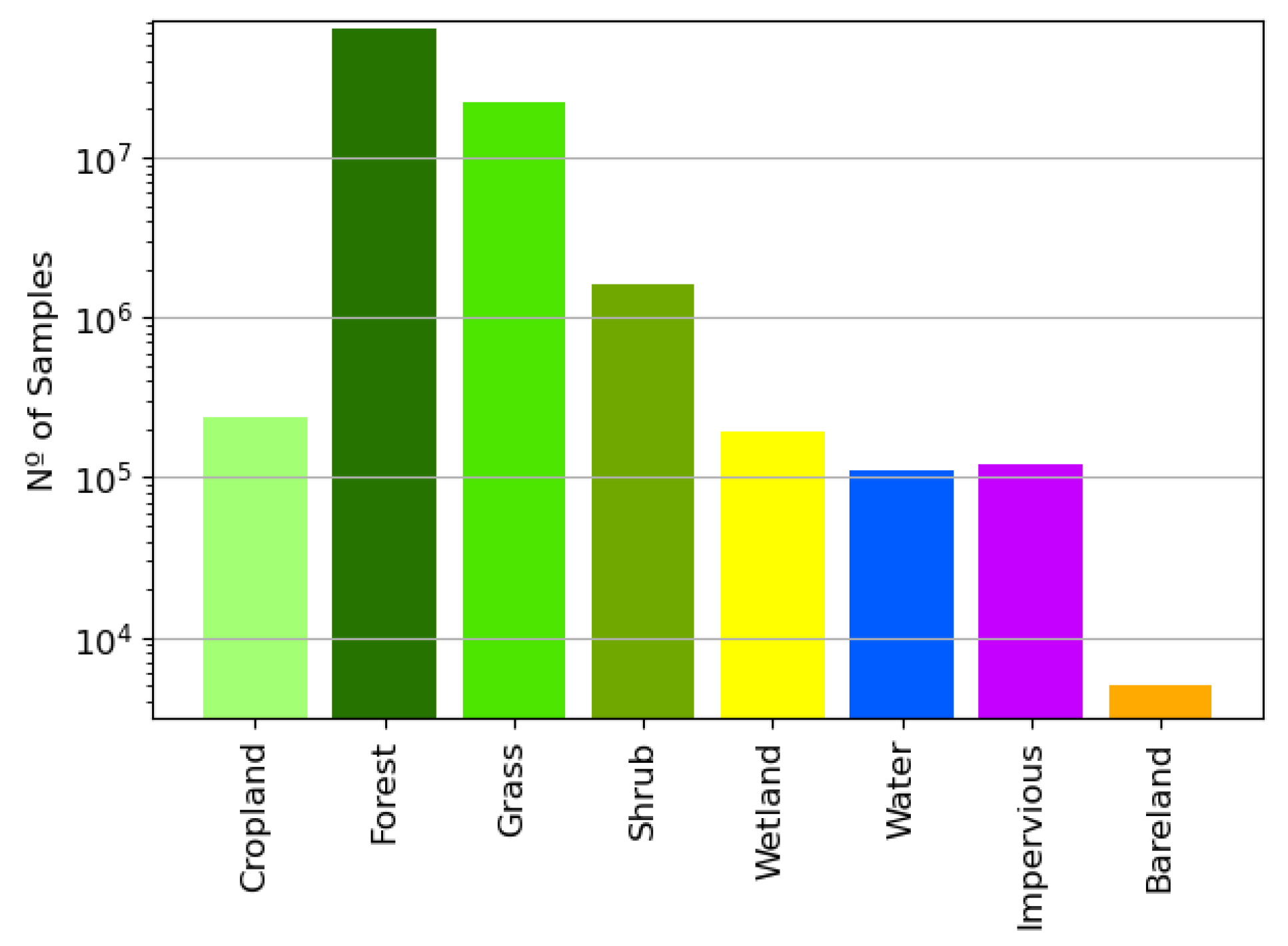
The 2017 FROM-GLC thematic map comprises a total of 10 land cover classes, namely Cropland, Forest, Grass, Shrub, Wetland, Water, Tundra, Impervious, Bareland, and Snow/Ice. Since Tundra and Snow/Ice are not present in the region of the Amazon Basin, eight FROM-GLC classes are represented within the swaths shown in Figure 1 and Table 2, as illustrated in Figure 3. In this scenario, the number of samples for each category is extremely imbalanced towards vegetated areas. For instance, a difference of up to four orders of magnitude can be observed when comparing the dominant Forest class with the minority one, i.e., the Bareland class.
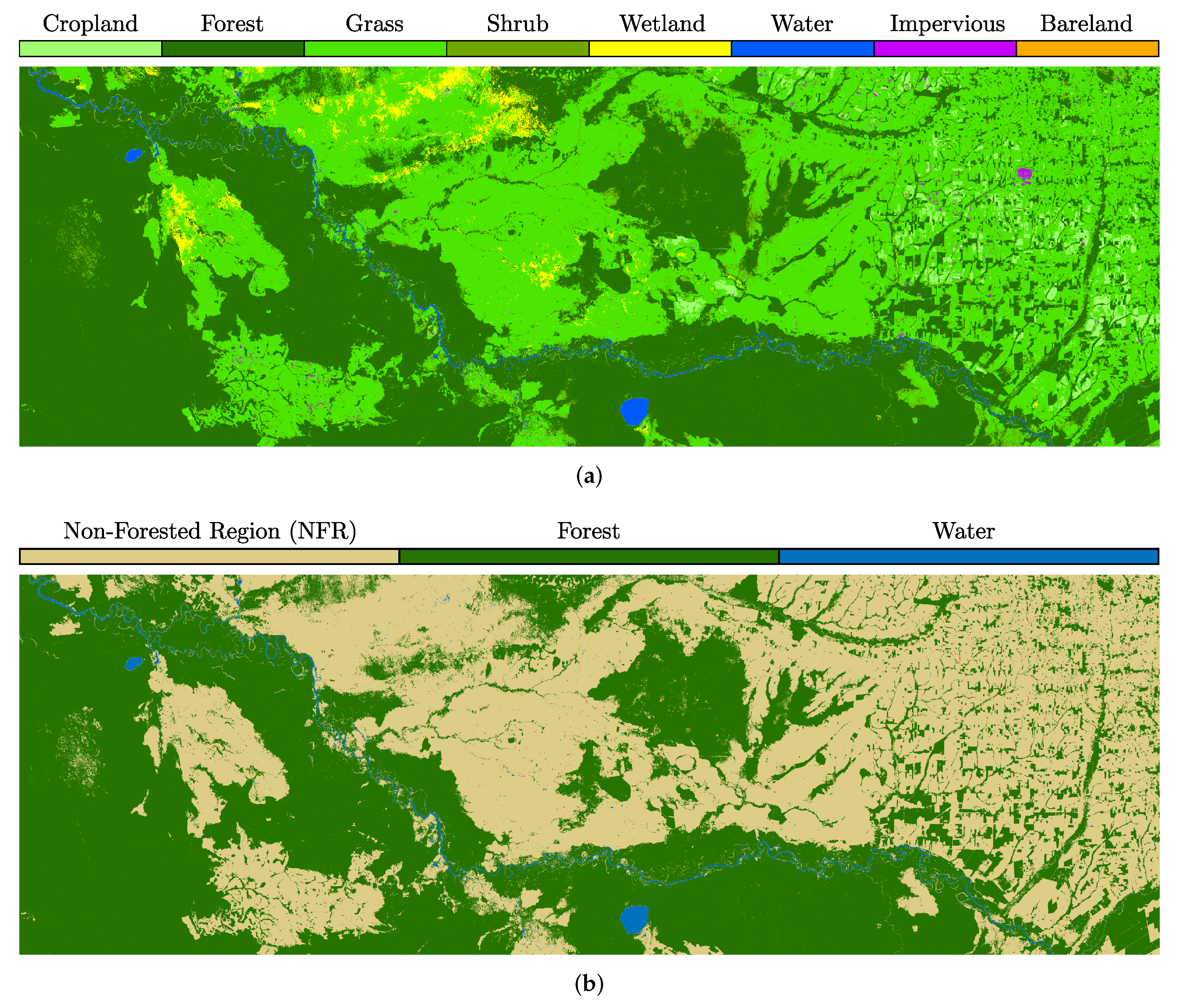
Classification of imbalanced datasets is highly challenging when training neural networks such as CNNs due to an undesired bias towards the dominant classes, i.e., since the training focuses on improving the classification accuracy, the prediction of classes with more samples tends to be more rewarding. Moreover, balancing a database for patch-based approaches such as the U-Net might be particularly difficult since an image patch containing minority classes will likely have samples from the dominant classes as well. In order to achieve a meaningful and robust training dataset, we decided to group the FROM-GLC classes Cropland, Grass, Shrub, Wetland, Impervious, and Bareland into a single higher-level one, the Non-Forested Region (NFR) class. In this way, we could still achieve our goal of monitoring the resources of greatest environmental interest within the Amazon Basin (Forest and Water classes). The original eight FROM-GLC classes and the adapted three higher-level ones considered in this paper are shown in Figure 4 for a cropped area within the swath from TS4010.
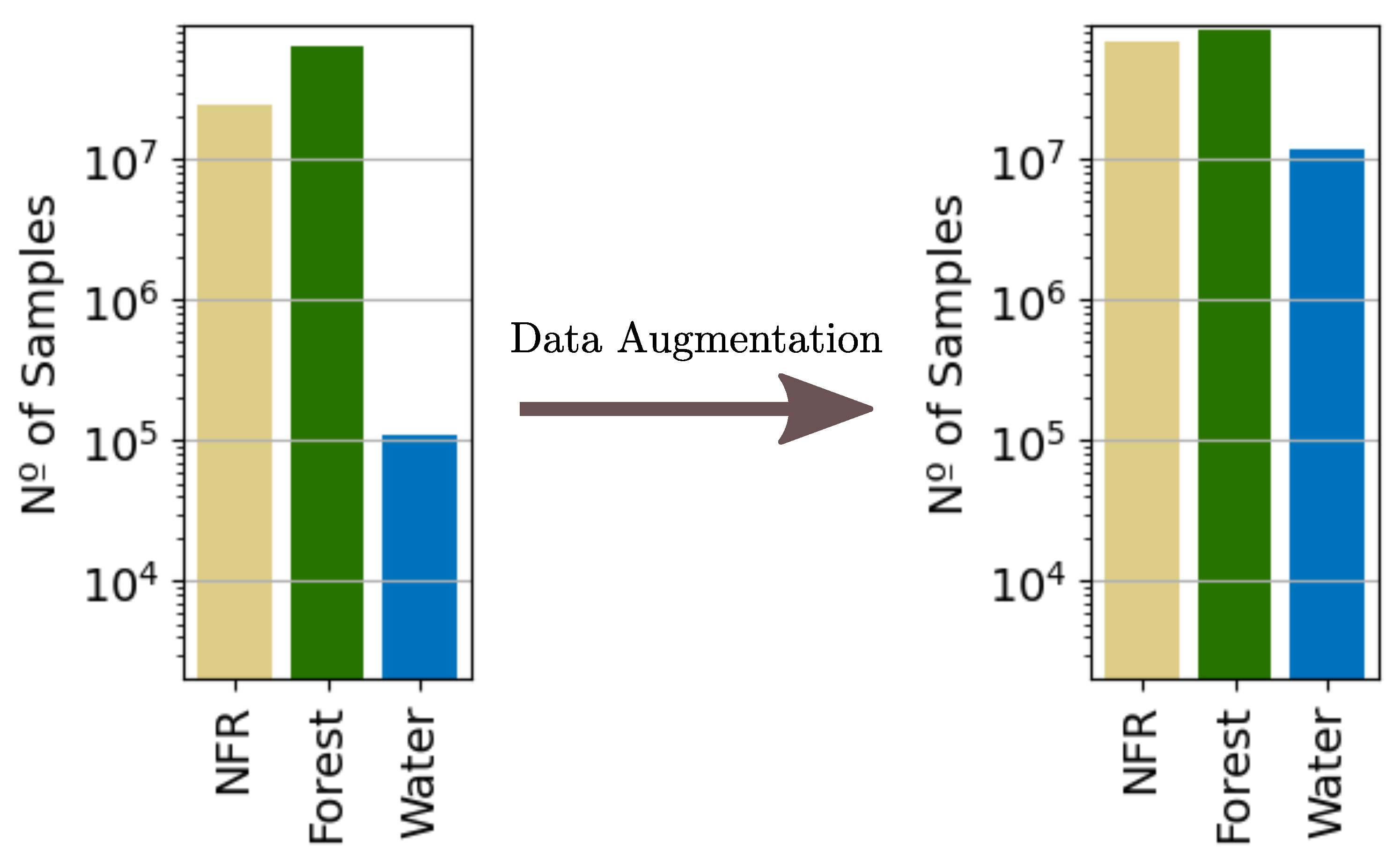
After the simplification of the FROM-GLC classes, an additional balancing course of action was performed to bring the three classes to the same order of magnitude through data augmentation. First, the NFR and Forest classes were undersampled by randomly removing patches where the Water class was absent. Then, data augmentation techniques were used to increase the number and diversity of the underrepresented Water class. The proposed patch-based augmentation included both horizontal and vertical flipping, as well as rotations with mirrored padding on the borders [17]. These techniques were chosen to maintain the pixelwise spatial relationship between labels and the input data—which could be affected by transformations that involve pixel interpolation. It should also be noted that, even after this processing, the database was not perfectly balanced since the oversampling of the minority class would likely have a similar effect on the dominant ones, as can be seen in Figure 5.
3. Methodology
In this section, we investigate the potential of CNNs for forest mapping by exploiting the evolution in time of S-1 interferometric STS. The objective was to exploit the powerful learning capabilities of a CNN to address some of the challenges that revolve around land cover classification with multi-temporal radar imagery over forests. For instance, the available number of reliable annotated samples for training remote sensing data is much smaller than in most computer vision problems, which might require the learning of higher-level features with respect to most applications. At the same time, given the unique nature of radar imaging and depending on the resolution cell size, there will be a high spatial dependency between neighboring pixels—and thus, it is desirable to keep track of these patterns and their localization on a pixel level. Hence, to comply with these requirements, we propose to use a convolution neural network based on the state-of-the-art U-Net architecture [19] to perform semantic segmentation of S-1 multi-temporal data.
3.1. Proposed U-Net-Like Classification Model
The U-Net was originally proposed to efficiently capture nuances required in the analysis of medical images, but has ever since become one of the standard tools for several classification problems, including land cover applications using spaceborne SAR data [18]. This architecture is based on a nearly symmetric encoder–decoder approach, which resembles a U-shaped structure: while the encoder part consists of a contraction path to capture context via feature extraction, the decoder is responsible for precisely retrieving spatial information along the upsampling, where the output of each convolutional level is combined with high-resolution features from the contraction path through skip connections.
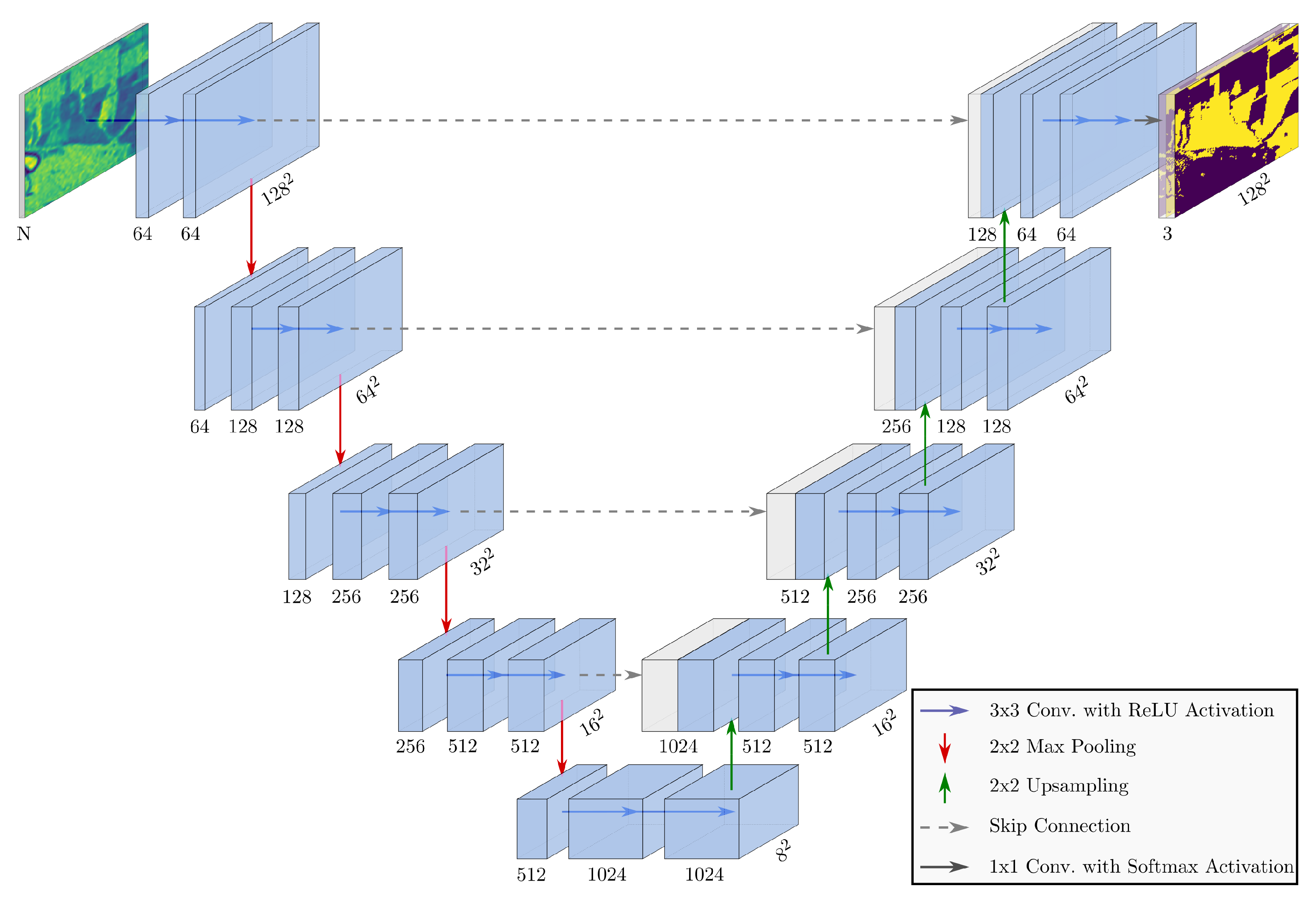
We now propose our own implementation of a U-Net-like architecture consisting of five convolutional levels, as shown in Figure 6. As the input, we considered patches of size 128 px × 128 px, stacked into N SAR and InSAR input feature channels. In the encoder path, each convolutional level consisted of two consecutive convolutions with a 3 × 3 kernel followed by a Rectified Linear Unit (ReLU) activation function. Then, we performed a 2 × 2 max pooling with stride 2 for downsampling. For the initial convolutional layer, we applied 64 filters (thus generating the same number of feature maps), which were doubled at each successive level. Moreover, differently from the original U-Net [19], our feature maps were not cropped after every convolution since we padded the borders with zero-valued pixels to keep the original image size at the output. On the decoder side, we performed an upsampling on every convolutional level by applying a 2 × 2 transposed convolution that halves the number of feature maps. These outputs were concatenated with the corresponding encoder features and, once again, went through two successive convolutions, each followed by a ReLU transformation. At the end of the network, a final layer uses a 1 × 1 convolution with a softmax activation function to perform the multi-layer semantic segmentation, mapping 64 features into the probability of each pixel to belong to the three classes of interest, i.e., Non-Forested Region, Forest, and Water. The class associated with the highest estimated probability would then be the one predicted by the network. This classification scheme was implemented in Python using the TensorFlow and Keras packages.
During the training phase, we used the cross-entropy between our annotated samples and the network’s predictions as the loss function that we wished to minimize. Moreover, since optimization algorithms tend to converge much faster when performing quick estimates of the gradient, we trained our algorithm utilizing batches of 32 randomly chosen image patches, from which we computed the average gradient. As the reparametrization method, we performed batch normalization after each convolutional level to better coordinate parameter updates across the layers. Finally, we selected the Adam algorithm [32] as our optimizer to iteratively adapt the network’s learning rate by using bias-corrected estimates of first- and second-order moments. This approach combines the advantages of both the Adaptive Gradient Algorithm (AdaGrad) [33] and Root-Mean-Squared Propagation (RMSProp) [34], being the standard optimization algorithm for several state-of-the-art CNNs.
3.2. Performance Evaluation Metrics
For the evaluation of the classification performance, we considered the following well-known pixelwise definitions:
- True Positive (TP): data points correctly assigned to their class, i.e., the predicted label is the same as the ground truth;
- True Negative (TN): correct rejection of a given class;
- False Positive (FP): data points mistakenly predicted as the class under consideration;
- False Negative (FN): incorrect rejection of a class.
These outcomes were used to calculate specific metrics for assessing the performance of a classification algorithm. In this paper, the following metrics were considered: precision, recall, F1-score, and accuracy, which are given by Equations (2)–(5), respectively:
Once these metrics are calculated for every class, we can compute their mean values in order to evaluate the macro performance of our classifiers. However, this analysis does not consider a potential class imbalance among the samples under test, as it weighs all classes equally. Thus, for a fairer global performance evaluation, we also estimate the overall statistics by computing the weighted average of each evaluation metric, with respect to the representativity of each class.
3.3. Experimental Setup
We evaluated the proposed classification model with different sets of input feature maps in order to provide a complete benchmark of their impact on the final classification performance and to compare the proposed framework with the baseline state-of-the-art algorithms. Thus, we divided the approaches under analysis into 10 different configurations, as summarized in Table 3. Case I is the baseline scheme presented in [23], which makes use of a random forest classifier with the following input features: the multi-temporal mean backscatter , the local incidence angle , the temporal decorrelation constant , the long-term coherence , and the local incidence angle . As mentioned in Section 2, both and were estimated in an exponential-model-fitting step to better characterize the temporal decorrelation between interferometric pairs. This approach was further exploited in [24], defined as case , where 18 additional texture features were estimated from the multi-temporal mean SAR backscatter to better describe the spatial dependency among neighboring pixels. The considered textures were: average, cluster prominence, cluster shade, contrast, correlation, energy, entropy, homogeneity, and variance. Each quantity was computed twice by considering displacement vectors along both the azimuth and the slant-range directions, respectively, whose mathematical formulation can be found in [24]. As for our convolutional neural network, we first tested it on case for the same input features considered in the baseline, in order to make a direct comparison. We skipped the texture estimation step, as it was expected that the network would be able to capture pixelwise spatial dependencies thanks to the two-dimensional convolutional layers. Then, in cases –X, we investigated if our approach was able to learn the temporal decorrelation trend by simply stacking in the input the interferometric coherence maps at different temporal baselines, where is the average among the four possible 6 d coherences, the average among the three 12 d coherences, the two averaged 18 d coherences, and simply the only available 24 d coherence. Each case considers a different combination of backscatter and coherence maps, although the local incidence angle is provided in all cases since the acquisition geometry impacts all the considered input features. Moreover, case makes use of the entire stack of multi-temporal coherence maps, but avoids the use of backscatter. Symmetrically, case V relies on backscatter information only. These two configurations were investigated in order to assess the additional value of combining both backscatter and coherence for improving the classification performance.
4. Results
The proposed algorithms were evaluated for the same dataset, i.e., swaths, considered in [24], in order to attain a fair comparison with the baseline technique. Thus, we used the four time series stacks from Orbit 083 shown in Figure 1 as our test set, while the remaining ones were allocated to the training set. In total, 9980 image patches of size 128 px × 128 px were used in the training phase, with 20% being randomly sampled for validation purposes. For each input feature configuration (cases to X in Table 3), we optimized the network with an initial learning rate of 10−3 and for 90 epochs.
Performance Evaluation
The numerical performance assessment of the Amazon Rainforest mapping was evaluated by considering the accuracy (see Equation (5)) and F1-score (see Equation (4)), which is the harmonic mean between precision and recall. These metrics were first individually computed for the classes NFR, Forest, and Water. Then, the total performance was summarized either by the mean values among these classes or by the overall statistics, as described in Section 3.2.
Table 4 shows the results for all 10 cases defined in Table 3. It can be seen that all CNN-based classification schemes outperformed the current state-of-the-art shallow learners from cases I [23] and [24] with the exception of case , in which we did not use any SAR backscatter information as the input. It should be noted that the random forests from cases I and were reproduced with the parameters defined in [24], which were optimized for the same STS used in our work. Thus, we used the Gini impurity to measure the quality of our splits, with a minimum of 50 samples per leaf node, for a random forest classifier composed of 50 trees. Moreover, from the results presented in Table 4, we can make the following considerations:
- Given a direct comparison (i.e., for the same baseline processing, training and test sets, and input features), the use of our CNN in case already achieved an improvement of more than five percentage points in both the overall F1-score and accuracy with respect to case I. Moreover, when comparing case to case , the performance gain was smaller—approximately 1.4 percentage points—but, most importantly, the computational load of case was extremely reduced since no specific computation of backscatter textures was required as in case ;
- Case and V make use of either the backscatter information or the stack of multi-temporal coherences, respectively, as input features to the CNN. In both cases, a small drop in the performance was visible with respect to all other CNN-based cases in which both backscatter and coherence were exploited. This confirmed the added value of combining both SAR intensity and interferometric information for classification purposes when utilizing STS;
- Case X achieved the best performance for every considered metric, although case might be deemed comparable in terms of F1-score and accuracy. Nevertheless, the required processing load was greatly reduced for case X, as both the backscatter texture estimation and the exponential model fitting of the temporal decorrelation were avoided in this setting. This suggests that the proposed CNN scheme was able to recognize by itself the temporal decorrelation patterns from the input multi-temporal coherence stacks;
- It should also be noted that even when the 6 d coherence stack was not considered (see case ), an overall F1-score and accuracy above 90% could be achieved. Therefore, this method could be successfully applied at a global scale, where only S-1 temporal baselines of at least 12 d (for a single Sentinel-1 satellite) are available, overcoming the limitations of [23,24], which required short temporal baselines for the theoretical modeling of the temporal decorrelation;
- From the analysis of cases from to X, it becomes clear that coherences at low temporal baselines allowed for the retrieval of a higher information content for the discrimination between forested and non-forested areas. This behavior was expected, since, if forests are severely decorrelated already at 6 d temporal baselines, at higher temporal baselines, non-vegetated areas appear almost completely decorrelated as well, increasing the confusion between these two classes. On the other hand, the long-term coherence at a 24 d temporal baseline remains very helpful for the discrimination of impervious areas, such as urban settlements, characterized by the presence of stable targets on the ground. This aspect is further discussed later on in Section 5.2;
- It is also important to point out that the test set still remained quite imbalanced, with a predominance of Forest samples and underrepresentation of Water ones. Therefore, the per-class metrics should be interpreted with caution. For instance, the Water class will have a high accuracy in all cases since minority classes tend to have a high number of true negatives.
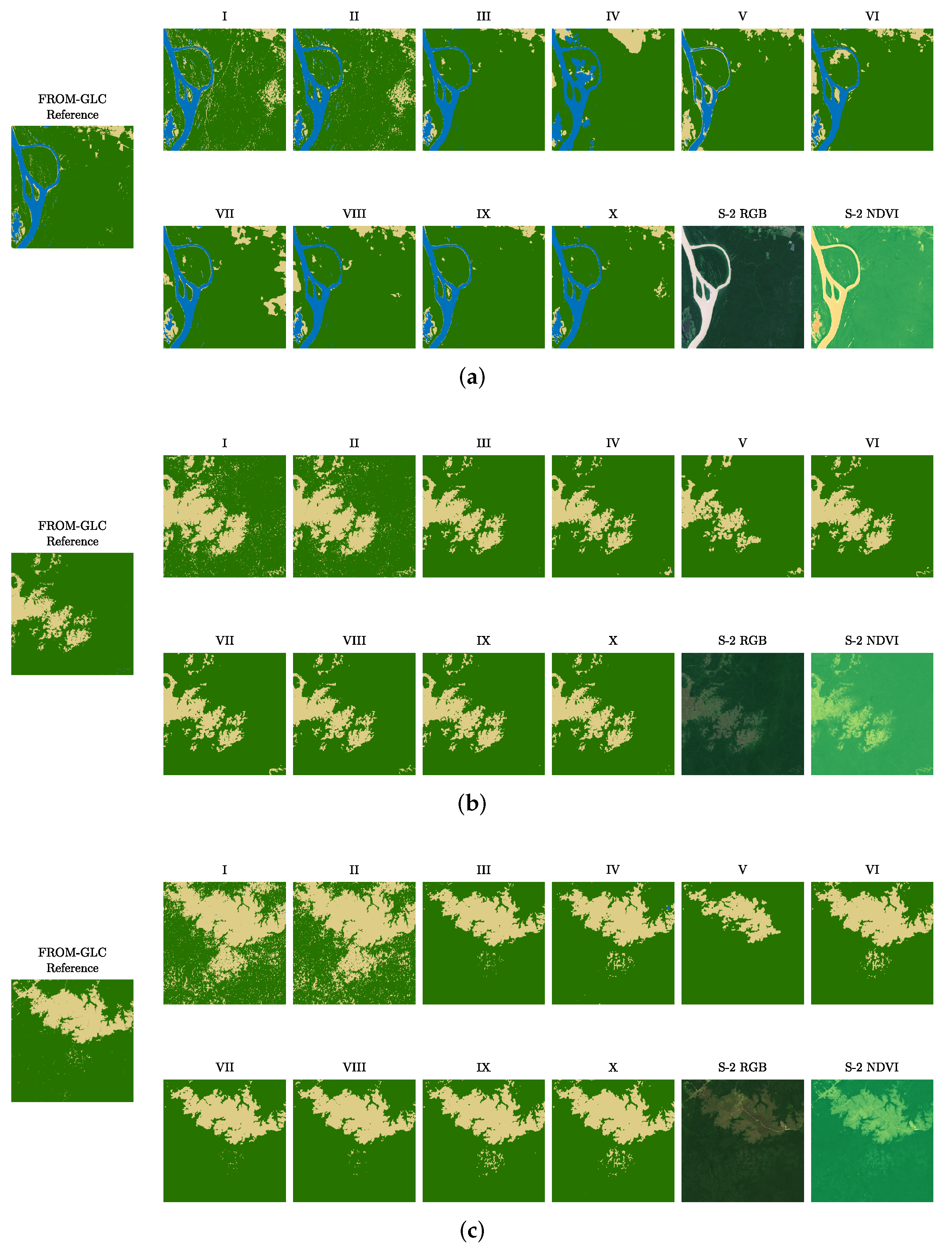
In Figure 7, we present a direct visual comparison between the FROM-GLC thematic map and the classification given by case X for the area in TS1083, as defined in Figure 1, which show a high level of agreement. Nevertheless, one can notice that roads appear slightly underestimated and often not completely connected. This effect was very likely related to the resolution of the input data (independent pixel spacing of about 70 m and final posting at 50 m), which mixes the signature of roads with the surroundings inside the same resolution cell. The same effect also happened in the presence of narrow river branches, which are only or less than a single pixel wide. We extended this analysis by performing a visual inspection of all proposed classification schemes against Sentinel-2 (S-2) RGB and NDVI images over a few regions from this swath. Thus, we selected three small image patches, delimited by the red squares and shown in greater detail in Figure 8, to illustrate some crucial differences between the 10 implemented classification approaches. Firstly, it can be noted that all CNN predictions were less noisy and more accurate than those from the random-forests-based approaches (cases I and ), which showed much more isolated misclassified pixels, especially over forested areas. This was probably due to the fact that the random forest classifier solely relies on pixelwise estimations, and the spatial information content of the data was limited to neighboring pixels only, which were utilized for the computation of the spatial textures. On the other hand, the CNN was able to consider a more extended spatial content in the data by relying on two-dimensional convolutional kernels. Moreover, the classification approach in case , which was the only case that did not rely on any kind of SAR backscatter information, struggled when mapping water surfaces. The latter result was slightly overestimated, which was probably caused by the fast temporal decorrelation of both water and forests, which led to similar low values in the coherence. On the other hand, this ambiguity was less prominent when adding the backscatter information. Indeed, rainforests at C-band are characterized by well-known values of around −6.4 dB [35], whereas calm water surfaces are close to the system noise floor [36]. Differently, in case V, where no coherence information was used, the classifier showed some inaccuracies when discriminating between forests and non-forested regions since they can both show very similar levels of backscatter. Finally, even though all the CNN approaches that make use of both SAR backscatter and any combination of interferometric coherences have a high agreement with the reference map, case X was the one able to capture most of the details, which was confirmed by visually comparing the three analyzed patches with the corresponding ones from the Sentinel-2 True Color RGB channel and the Normalized Difference Vegetation Index (NDVI), which represents a good indicator of the presence of green vegetation [37].
Finally, we provide some details on the computational times for the processing of a single STS, as described in Section 2.2. The test was performed using a 24 Core Intel(R) Xeon(R) CPU E5-2690 v3 @ 2.60 GHz, with 512 GB RAM. The core SAR and InSAR processing, which includes coregistration, multi-temporal backscatter and coherence matrix computation, and geocoding lasted overall 2h21. This was the pre-processing time required for the generation of all input features for the experimental setup cases from to X. Additionally, the computation of the temporal decorrelation and the exponential fitting (as in cases I to ) required 2h:42, while the computation of backscatter textures (as in case ) lasted 26. By avoiding the use of both textures and temporal decorrelation fitting parameters, the overall computational time for this processing phase could be reduced by 3h8, which corresponds to more than 57% of the overall processing time.
5. Discussion
In Section 4, we showed that, by relying on the powerful learning capabilities of a U-Net-like CNN model, it was possible to simplify the baseline short time series processing and classification chain proposed in [23,24] while still achieving an even higher agreement with the external reference map. We now draw a series of considerations on the proposed approach, aiming at exploring further research perspectives and possibilities for land cover classification using S-1 STS.
5.1. Class Assignment and Potential Confusion Sources
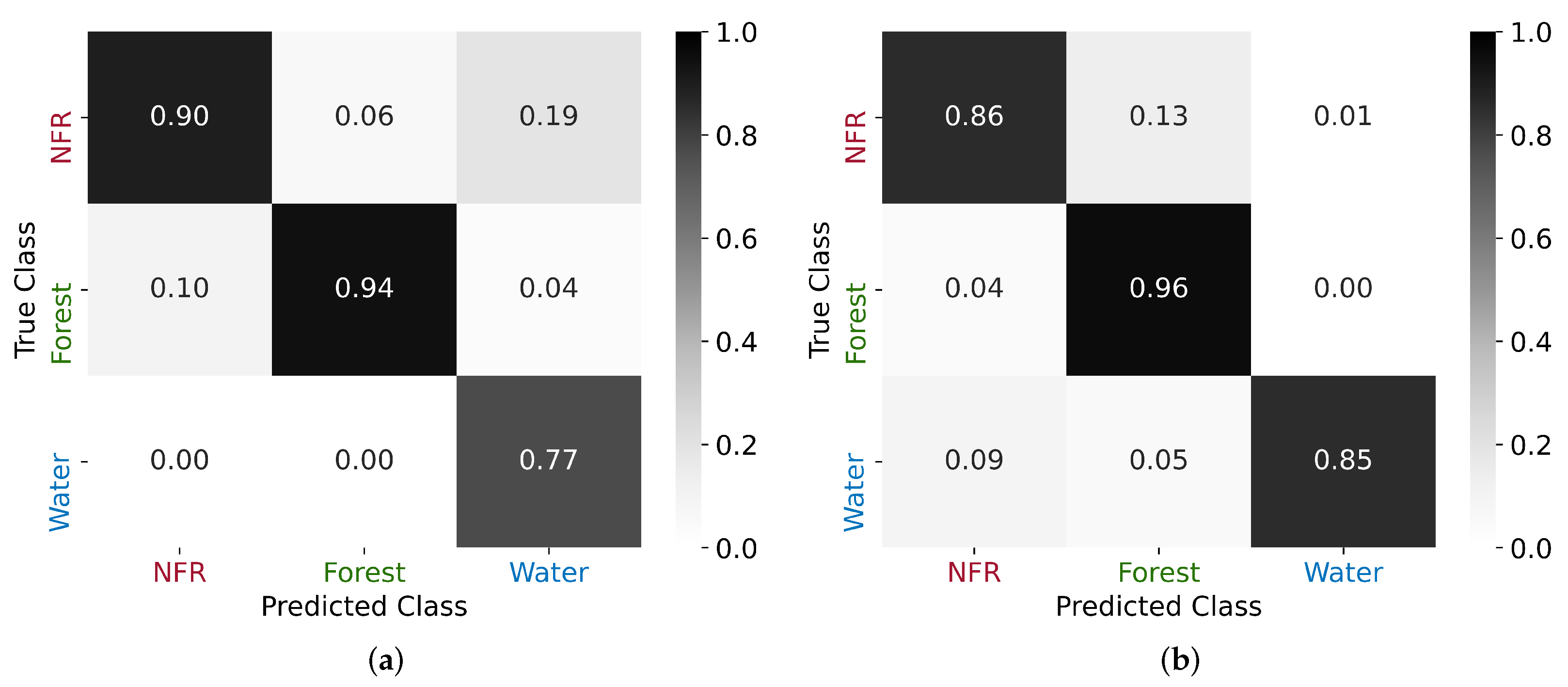
Firstly, we investigated the reasons for the occurrence of misclassifications in our proposed approaches. To do so, we analyzed the confusion matrices, shown in Figure 9, for the best-case scenario (i.e., case X in Table 4). Since our test set was extremely imbalanced towards the Forest class, for a better visualization, we display two confusion matrices normalized by the predicted and true classes, respectively. Thus, each confusion matrix provides a different insight of how each class was misclassified. Figure 9a should be interpreted columnwise only, and for the total predictions of each class, it shows the proportion of the actual annotated samples. Analogously, Figure 9b must be analyzed per row, and in this case, for the totality of samples belonging to each class, it provides the ratio of predictions made towards NFR, Forest, or Water. In this way, it should be noted that the main diagonal in Figure 9a represents the classifier’s precision, while in Figure 9b, it represents its recall. Moreover, we can see in the first case that 19% of the Water class predictions actually belonged to the NFR class, which could be mainly explained by the fact that smaller Amazon River branches might be only a single-pixel wide due to limitations in the resolution of S-1 data. This was also the reason why most mispredictions happened along their riverbanks.
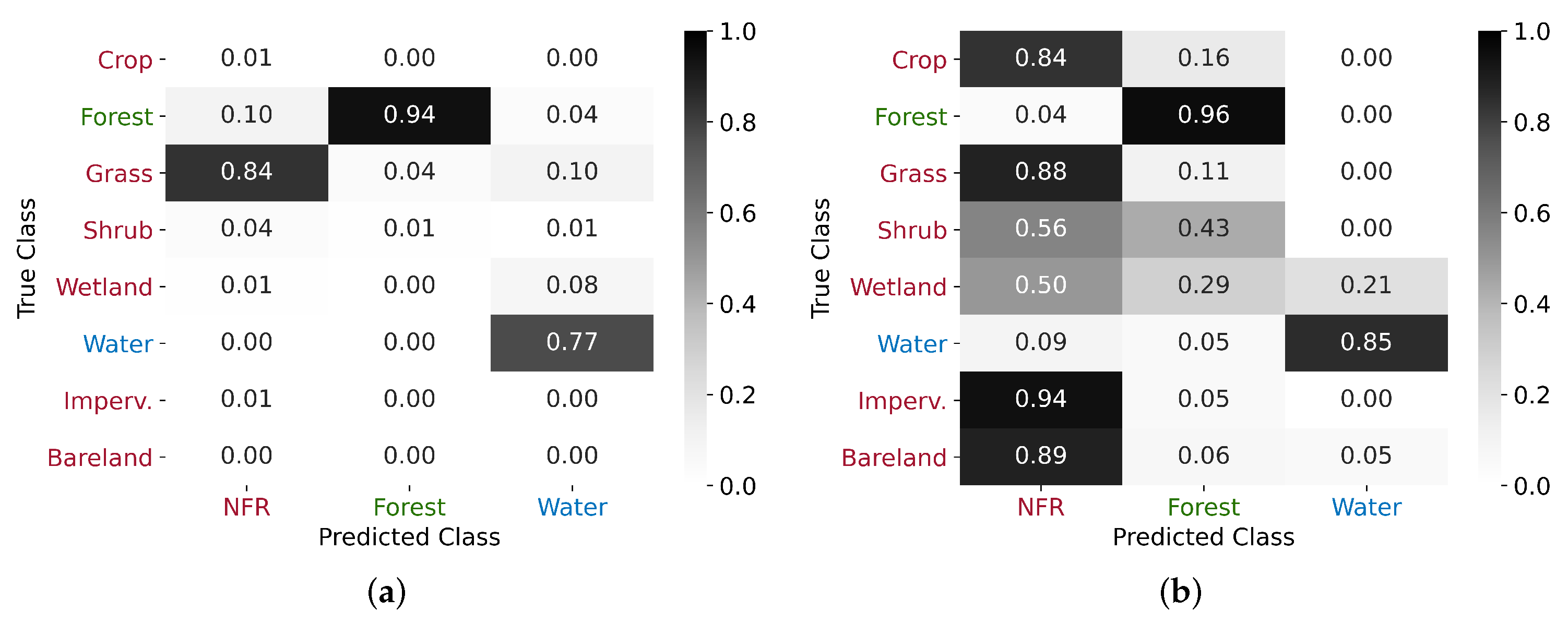
This analysis was further explored in the normalized confusion matrices shown in Figure 10, where we checked our predictions against the eight original FROM-GLC classes. In this way, we can verify the robustness of our higher-level class grouping approach and identify a posteriori patterns in the mispredictions. It can be seen that the Shrub and Wetland classes represented the greatest sources of confusion. The Shrub class is characterized by the presence of bushes or shorter trees, being often associated with the Forest class. This aspect suggests that, similarly to X-Band [14], also C-Band InSAR data are sensitive to the presence of sparse and low vegetation, which impacts the S-1 multi-temporal coherence through a fast decorrelation in time. Regarding the Wetland class, it is characterized by a fast-changing nature, especially during the wet season, which might explain the network’s poor performance when attempting to classify it.
5.2. Impervious Areas and the Role of Short- and Long-Term Coherences
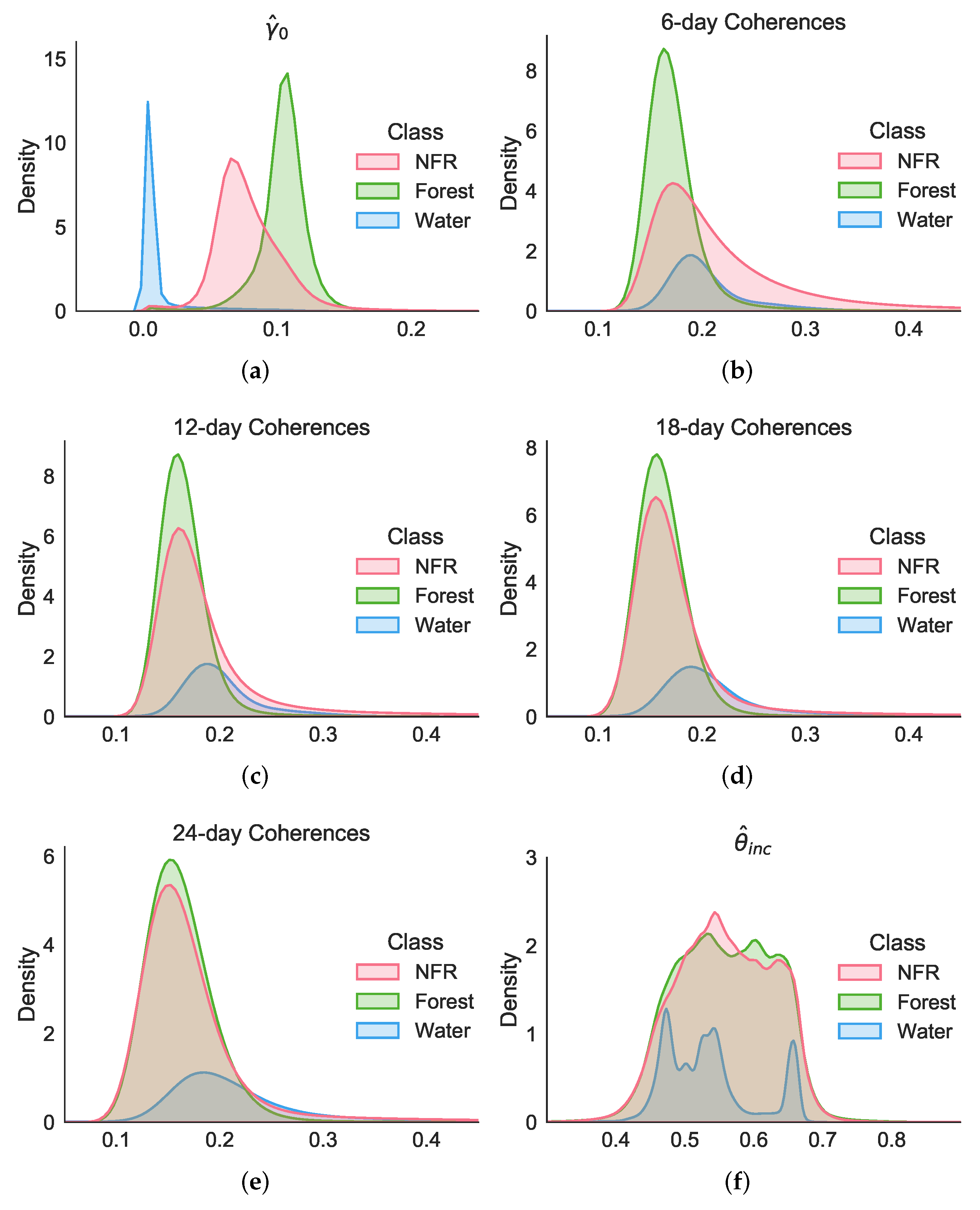
We saw in Section 2 the challenges of dealing with an imbalanced dataset, which led us to define only three high-level classes of interest for mapping the Amazon Rainforest: NFR, Forest, and Water. In Figure 11, we show the normalized histograms of each of these classes for the average SAR backscatter, the interferometric coherences at different temporal baselines, as well as the local incidence angle.
The distributions shown in Figure 11 confirmed that the backscatter information was crucial for discriminating all three classes, given the clear separation among the different distributions. Furthermore, the coherence stacks were overall more useful in this task for the shortest temporal baseline, i.e., the 6 d coherences.
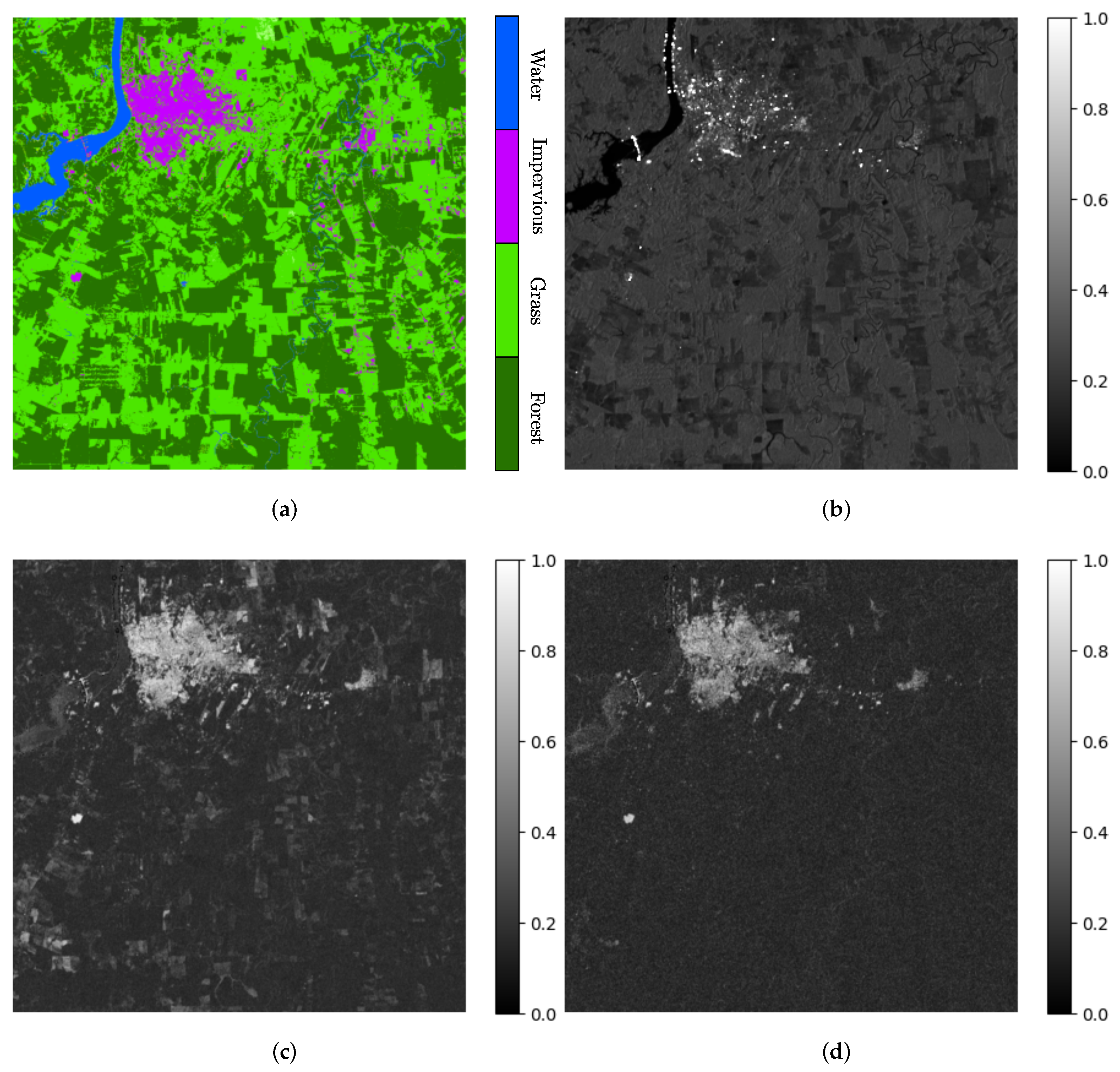
However, when moving to more heterogeneous areas, we could expect to redefine how the classes are grouped together depending not only on the available number of samples, but also on the application of interest. For instance, in more populated areas, a possible task could be to monitor urban expansion. In this case, the Impervious class could be considered as a separate one, as shown for the metropolitan area of Porto Velho in Figure 12. Indeed, from the 6 d mean coherence in Figure 12c, one can appreciate how low-vegetated areas still showed some degree of correlation with respect to forested ones, which, on the other hand, were already severely decorrelated. From Figure 12d, the role of the long-term coherence at the 24 d temporal baseline to discriminate urban settlements and human-made structures becomes clear, which still showed high values of coherence thanks to the temporal stability of the targets on the ground.
6. Conclusions and Outlook
In this paper, we investigated the potential of deep learning for performing land cover classification over forested areas with repeat-pass interferometric SAR data. In particular, we combined openly available Sentinel-1 time series with short temporal baselines, together with the learning capabilities of a U-Net-like convolutional neural network to map forests, non-forested regions, and water surfaces in the Amazon Basin. The results of this study showed that, by using the proposed deep learning model, we were able to skip two computationally costly steps from the baseline processing chain—the texture estimation and exponential model fitting—and still outperform the state-of-the-art shallow learning classifiers for S-1 short time series. We obtained the best classification performance by considering the full stack of coherence maps at different temporal baselines (from 6 d up to 24 d) as input features to the CNN, together with the multi-temporal mean backscatter. Nevertheless, a good overall performance was also obtained when considering coherence stacks with a minimum temporal baseline of 12 d. The advantage of this last configuration is that it can be utilized for monitoring forests at a global scale since Sentinel-1 InSAR data at a 6 d revisit time is only operationally available over Europe or dedicated test sites. Furthermore, one of the greatest assets of our approach is the possibility to generate accurate forest maps within a temporal baseline of less than a month, allowing for an effective monitoring of rainforests. This aspect represents a significant improvement with respect to current operational forest monitoring systems, which typically require much longer observation intervals for the generation of large-scale forest mapping products. A monthly update will allow us to properly follow dynamic changes in forest coverage caused, e.g., by deforestation and forest degradation phenomena. Moreover, by solely relying on radar data, gap-free products can be regularly generated, overcoming the limitation of optical sensors for the monitoring of cloudy regions, such as tropical forests. The proposed framework is currently at a prototype stage and needs further developments to be brought to an operational stage. Regarding this aspect, we will concentrate further efforts on the understanding of how fast-changing seasonal effects within the Amazon Basin (e.g., the dynamics of floods and droughts or vegetation phenology) could affect our training and predictions over the course of a year. If this impact is shown to be significant when testing the proposed approach over a longer period and on a larger scale, our training strategy might have to be refined by including such information within the ancillary reference data and fine-tuning the proposed CNN model.
Author Contributions
Conceptualization, R.D.M.J. and P.R.; methodology, R.D.M.J. and P.R.; software, R.D.M.J.; validation, R.D.M.J.; formal analysis, R.D.M.J. and P.R.; investigation, R.D.M.J. and P.R.; resources, R.D.M.J. and P.R.; data curation, R.D.M.J. and P.R.; writing—original draft preparation, R.D.M.J.; writing—review and editing, P.R.; visualization, R.D.M.J. and P.R.; supervision, P.R.; project administration, P.R.; funding acquisition, P.R. All authors have read and agreed to the published version of the manuscript.
Funding
This research received no external funding.
Institutional Review Board Statement
Not applicable.
Informed Consent Statement
Not applicable.
Data Availability Statement
Sentinel-1 data used in this work are available at The Copernicus Open Access Hub: https://scihub.copernicus.eu/, accessed on 4 October 2021. Moreover, the FROM-GLC thematic maps chosen as external reference data can be found at: http://data.ess.tsinghua.edu.cn, accessed on 4 October 2021.
Acknowledgments
The authors would like to thank our colleagues Andrea Pulella and Francescopaolo Sica for the collaboration at the early stages of this study and Luca Dell’Amore and José-Luis Bueso-Bello for the support during the entire project. Moreover, we would like to thank ESA once again for the acquisition of the Amazon dataset at a 6 d repeat-pass.
Conflicts of Interest
The authors declare no conflict of interest.
References
- FAO. Global Forest Resources Assessment 2020: Main report; FAO: Rome, Italy, 2020; p. 184. [Google Scholar]
- Bravo, F.; Jandl, R.; LeMay, V.; Gadow, K. Managing Forest Ecosystems: The Challenge of Climate Change; Springer International Publishing: New York, NY, USA, 2008; p. 452. [Google Scholar]
- FAO; UNEP. The State of the World’s Forests 2020: Forests, Biodiversity and People; FAO and UNEP: Rome, Italy, 2020; p. 214. [Google Scholar]
- Lawrence, D.; Vandecar, K. Effects of tropical deforestation on climate and agriculture. Nat. Clim. Chang. 2015, 5, 27–36. [Google Scholar] [CrossRef]
- Monitoramento do Desmatamento da Floresta Amazônica Brasileira por Satélite. Available online: http://www.obt.inpe.br/OBT/assuntos/programas/amazonia/prodes (accessed on 26 August 2021).
- Diniz, C.G.; Souza, A.A.d.A.; Santos, D.C.; Dias, M.C.; Luz, N.C.d.; Moraes, D.R.V.d.; Maia, J.S.; Gomes, A.R.; Narvaes, I.d.S.; Valeriano, D.M.; et al. DETER-B: The New Amazon Near Real-Time Deforestation Detection System. IEEE J. Sel. Top. Appl. Earth Obs. Remote Sens. 2015, 8, 3619–3628. [Google Scholar] [CrossRef]
- Almeida, C.A.d.; Coutinho, A.C.; Esquerdo, J.C.D.M.; Adami, M.; Venturieri, A.; Diniz, C.G.; Dessay, N.; Durieux, L.; Gomes, A.R. High spatial resolution land use and land cover mapping of the Brazilian Legal Amazon in 2008 using Landsat-5/TM and MODIS data. Acta Amaz. 2016, 46, 291–302. [Google Scholar] [CrossRef]
- de Bem, P.P.; de Carvalho Junior, O.A.; Fontes Guimarães, R.; Trancoso Gomes, R.A. Change Detection of Deforestation in the Brazilian Amazon Using Landsat Data and Convolutional Neural Networks. Remote Sens. 2020, 12, 901. [Google Scholar] [CrossRef] [Green Version]
- Doblas, J.; Shimabukuro, Y.; Sant’Anna, S.; Carneiro, A.; Aragão, L.; Almeida, C. Optimizing Near Real-Time Detection of Deforestation on Tropical Rainforests Using Sentinel-1 Data. Remote Sens. 2020, 12, 3922. [Google Scholar] [CrossRef]
- Shimada, M.; Itoh, T.; Motooka, T.; Watanabe, M.; Shiraishi, T.; Thapa, R.; Lucas, R. New global forest/non-forest maps from ALOS PALSAR data (2007–2010). Remote Sens. Environ. 2014, 155, 13–31. [Google Scholar] [CrossRef]
- Reiche, J.; Mullissa, A.; Slagter, B.; Gou, Y.; Tsendbazar, N.E.; Odongo-Braun, C.; Vollrath, A.; Weisse, M.J.; Stolle, F.; Pickens, A.; et al. Forest disturbance alerts for the Congo Basin using Sentinel-1. Environ. Res. Lett. 2021, 16, 024005. [Google Scholar] [CrossRef]
- Copernicus Sentinel-1. Available online: https://sentinels.copernicus.eu/web/sentinel/missions/sentinel-1 (accessed on 3 September 2021).
- Krieger, G.; Moreira, A.; Fiedler, H.; Hajnsek, I.; Werner, M.; Younis, M.; Zink, M. TanDEM-X: A satellite formation for high-resolution SAR interferometry. IEEE Trans. Geosci. Remote Sens. 2007, 45, 3317–3341. [Google Scholar] [CrossRef] [Green Version]
- Martone, M.; Rizzoli, P.; Wecklich, C.; González, C.; Bueso-Bello, J.L.; Valdo, P.; Schulze, D.; Zink, M.; Krieger, G.; Moreira, A. The global forest/non-forest map from TanDEM-X interferometric SAR data. Remote Sens. Environ. 2018, 205, 352–373. [Google Scholar] [CrossRef]
- Kuck, T.N.; Sano, E.E.; Bispo, P.d.C.; Shiguemori, E.H.; Silva Filho, P.F.F.; Matricardi, E.A.T. A Comparative Assessment of Machine-Learning Techniques for Forest Degradation Caused by Selective Logging in an Amazon Region Using Multitemporal X-Band SAR Images. Remote Sens. 2021, 13, 3341. [Google Scholar] [CrossRef]
- COSMO-SkyMed Mission and Products Description. Available online: https://earth.esa.int/eogateway/documents/20142/37627/COSMO-SkyMed-Mission-Products-Description.pdf (accessed on 4 October 2021).
- Goodfellow, I.; Bengio, Y.; Courville, A. Deep Learning; MIT Press: Cambridge, UK, 2016. [Google Scholar]
- Mazza, A.; Sica, F.; Rizzoli, P.; Scarpa, G. TanDEM-X forest mapping using convolutional neural networks. Remote Sens. 2019, 11, 2980. [Google Scholar] [CrossRef] [Green Version]
- Ronneberger, O.; Fischer, P.; Brox, T. U-Net: Convolutional Networks for Biomedical Image Segmentation. In Medical Image Computing and Computer-Assisted Intervention—MICCAI 2015; Navab, N., Hornegger, J., Wells, W.M., Frangi, A.F., Eds.; Springer International Publishing: Cham, Switzerland, 2015; pp. 234–241. [Google Scholar]
- Huang, G.; Liu, Z.; van der Maaten, L.; Weinberger, K.Q. Densely Connected Convolutional Networks. In Proceedings of the IEEE Conference on Computer Vision and Pattern Recognition (CVPR), Honolulu, HI, USA, 22–25 July 2017. [Google Scholar]
- He, K.; Zhang, X.; Ren, S.; Sun, J. Deep Residual Learning for Image Recognition. In Proceedings of the IEEE Conference on Computer Vision and Pattern Recognition (CVPR), Las Vegas, NV, USA, 27–30 June 2016. [Google Scholar]
- De Zan, F.; Monti Guarnieri, A. TOPSAR: Terrain Observation by Progressive Scans. IEEE Trans. Geosci. Remote Sens. 2006, 44, 2352–2360. [Google Scholar] [CrossRef]
- Sica, F.; Pulella, A.; Nannini, M.; Pinheiro, M.; Rizzoli, P. Repeat-pass SAR interferometry for land cover classification: A methodology using Sentinel-1 Short-Time-Series. Remote Sens. Environ. 2019, 232, 111277. [Google Scholar] [CrossRef]
- Pulella, A.; Aragão Santos, R.; Sica, F.; Posovszky, P.; Rizzoli, P. Multi-Temporal Sentinel-1 Backscatter and Coherence for Rainforest Mapping. Remote Sens. 2020, 12, 847. [Google Scholar] [CrossRef] [Green Version]
- Unser, M. Sum and Difference Histograms for Texture Classification. IEEE Trans. Pattern Anal. Mach. Intell. 1986, PAMI-8, 118–125. [Google Scholar] [CrossRef] [PubMed]
- Ferretti, A.; Prati, C.; Rocca, F. Permanent scatterers in SAR interferometry. IEEE Trans. Geosci. Remote Sens. 2001, 39, 8–20. [Google Scholar] [CrossRef]
- Jacob, A.W.; Vicente-Guijalba, F.; Lopez-Martinez, C.; Lopez-Sanchez, J.; Litzinger, M.; Kristen, H.; Mestre-Quereda, A.; Ziolkowski, D.; Lavalle, M.; Notarnicola, C.; et al. Sentinel-1 InSAR Coherence for Land Cover Mapping: A Comparison of Multiple Feature-Based Classifiers. IEEE J. Sel. Top. Appl. Earth Obs. Remote Sens. 2020, 13, 535–552. [Google Scholar] [CrossRef] [Green Version]
- Batistella, M.; Robeson, S.; Moran, E. Settlement Design, Forest Fragmentation, and Landscape Change in Rondonia, Amazonia. Photogramm. Eng. Remote Sens. 2003, 69, 805–812. [Google Scholar] [CrossRef] [Green Version]
- Prats, P.; Rodriguez-Cassola, M.; Marotti, L.; Nannini, M.; Wollstadt, S.; Schulze, D.; Tous-Ramon, N.; Younis, M.; Krieger, G.; Reigber, A. TAXI: A Versatile Processing Chain for Experimental TanDEM-X Product Evaluation. In Proceedings of the IEEE Geoscience and Remote Sensing Symposium, Honolulu, HI, USA, 25–30 July 2010; pp. 1–4. [Google Scholar]
- Yague-Martinez, N.; Prats-Iraola, P.; Gonzalez, F.R.; Brcic, R.; Shau, R.; Geudtner, D.; Eineder, M.; Bamler, R. Interferometric processing of Sentinel-1 TOPS data. IEEE Trans. Geosci. Remote Sens. 2016, 54, 2220–2234. [Google Scholar] [CrossRef] [Green Version]
- Gong, P.; Liu, H.; Zhang, M.; Li, C.; Wang, J.; Huang, H.; Clinton, N.; Ji, L.; Li, W.; Bai, Y.; et al. Stable classification with limited sample: Transferring a 30-m resolution sample set collected in 2015 to mapping 10-m resolution global land cover in 2017. Sci. Bull. 2019, 64, 370–373. [Google Scholar] [CrossRef] [Green Version]
- Kingma, D.; Ba, J. Adam: A Method for Stochastic Optimization. arXiv 2014, arXiv:1412.6980. [Google Scholar]
- Duchi, J.; Hazan, E.; Singer, Y. Adaptive Subgradient Methods for Online Learning and Stochastic Optimization. J. Mach. Learn. Res. 2011, 12, 2121–2159. [Google Scholar]
- Tieleman, T.; Hinton, G. Lecture 6.5-rmsprop: Divide the gradient by a running average of its recent magnitude. Coursera Neural Netw. Mach. Learn. 2012, 4, 26–31. [Google Scholar]
- Hawkings, R.; Attema, E.; Crapolicchio, R.; Lecomte, P.; Closa, J.; Meadows, P.; Srivastava, S.K. Stability of Amazon Backscatter at C-Band: Spaceborne Results from ERS-1/2 and RADARSAT-1. In Proceedings of the CEOS SAR Workshop 1999, Toulouse, France, 26–29 October 2000. [Google Scholar]
- Piantanida, R.; Miranda, N.; Franceschi, N.; Meadows, P. Thermal Denoising of Products Generated by the S-1 IPF; Technical Report; European Space Agency (ESA): Paris, France, 2017. [Google Scholar]
- Rees, G. The Remote Sensing Data Book; Cambridge University Press: Cambridge, UK, 1999. [Google Scholar]
Figure 1.
Study sites in the Amazon Forest comprising the Brazilian states of Rondônia, Amazonas, and Mato Grosso, as well as smaller regions in Bolivia. In total, 12 swaths were considered for mapping the Amazon Rainforest by processing S-1 interferometric STS, divided according to relative orbits 010, 054, 083, and 156. The considered footprints are superimposed on an aerial scene from Google Earth.

Figure 2.
Short time series processing chain as developed in [24]. Our goal was to reduce the processing time required for classifying S-1 InSAR images by skipping the texture estimation and exponential model fitting steps (highlighted using dashed lines). To this end, we propose a CNN for automatically learning relevant features.

Figure 3.
Available number of samples, i.e., pixels, within the 12 interferometric short time series stacks defined in Table 2 for every class considered in the FROM-GLC thematic maps. The class imbalance is a challenge for training and validating neural networks, as a prediction bias favors the detection of dominant classes.

Figure 4.
Cropped region from the TS4010 swath, displaying (a) the highly imbalanced original eight FROM-GLC classes and (b) the three higher-level classes considered in this paper: Non-Forested Region (NFR), Forest, and Water.
Figure 4.
Cropped region from the TS4010 swath, displaying (a) the highly imbalanced original eight FROM-GLC classes and (b) the three higher-level classes considered in this paper: Non-Forested Region (NFR), Forest, and Water.

Figure 5.
Original number of samples for each of the three high-level classes of interest (left) and data availability after balancing (right). We artificially augmented Water patches and undersampled the ones dominated by the NFR and Forest classes.
Figure 5.
Original number of samples for each of the three high-level classes of interest (left) and data availability after balancing (right). We artificially augmented Water patches and undersampled the ones dominated by the NFR and Forest classes.

Figure 6.
U-Net-like architecture proposed for mapping the Amazon Basin.

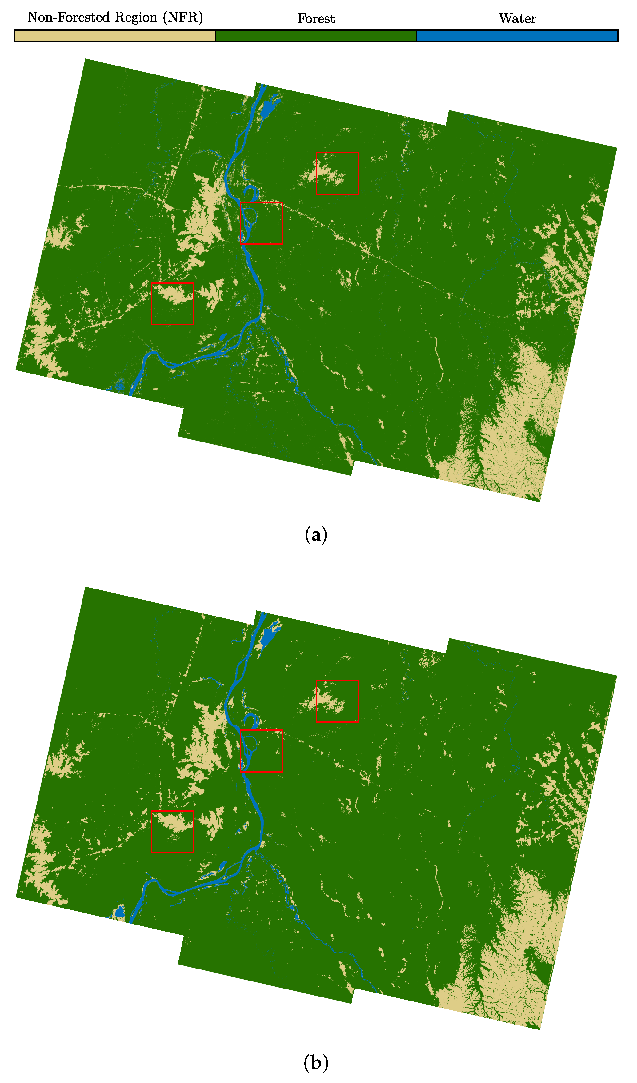
Figure 7.
Comparison of (a) the FROM-GLC reference map and (b) the prediction for case X from the area in TS1083. We selected three image patches of size 384 px × 384 px to perform a detailed visual inspection for all the 10 cases under analysis.
Figure 7.
Comparison of (a) the FROM-GLC reference map and (b) the prediction for case X from the area in TS1083. We selected three image patches of size 384 px × 384 px to perform a detailed visual inspection for all the 10 cases under analysis.

Figure 8.
Comparison of the proposed approaches for the three patches (a–c) defined in Figure 7.
Figure 8.
Comparison of the proposed approaches for the three patches (a–c) defined in Figure 7.

Figure 9.
Confusion matrices for the CNN scheme proposed in case X: (a) normalized by the predicted class and (b) normalized by the true class.
Figure 9.
Confusion matrices for the CNN scheme proposed in case X: (a) normalized by the predicted class and (b) normalized by the true class.

Figure 10.
Confusion matrices normalized by (a) the predicted and (b) the true classes, considering the original labels of the eight available FROM-GLC classes.
Figure 10.
Confusion matrices normalized by (a) the predicted and (b) the true classes, considering the original labels of the eight available FROM-GLC classes.

Figure 11.
Normalized histograms of (a) the SAR backscatter, (b–e) the interferometric coherence at different temporal baselines, and (f) the local incidence angle.
Figure 11.
Normalized histograms of (a) the SAR backscatter, (b–e) the interferometric coherence at different temporal baselines, and (f) the local incidence angle.

Figure 12.
Metropolitan area of Porto Velho, capital of the state of Rondônia, shown according to: (a) the FROM-GLC thematic map, (b) average SAR backscatter, (c) 6 d coherence, and (d) 24 d coherence. In this case, the long-term coherence is more suitable for the detection of impervious (e.g., urban) areas.


Table 1.
Sentinel-1 platform and interferometric acquisition parameters.
| Parameter | Value |
|---|---|
| Satellite platform | Sentinel-1A, Sentinel-1B |
| Orbital node | Descending |
| Acquisition mode | Interferometric Wide Swath (IW) |
| Center frequency | 5.405 GHz, C-band |
| Data product | Single-Look Complex (SLC) images |
| Revisit time | 6 d |
Table 2.
Description of the 12 Time Series (TS) stacks, their relative orbits, acquisition dates, and corner coordinates of the swaths.
Table 2.
Description of the 12 Time Series (TS) stacks, their relative orbits, acquisition dates, and corner coordinates of the swaths.
| Stack[orbit] | Observation Period | Master Date | Center Coordinates | |
|---|---|---|---|---|
| Latitude | Longitude | |||
| TS1010 | 25.04.19–19.05.19 | 07.05.19 | 8°43′22.08″ S | 60°48′27.36″ W |
| TS2010 | 10°14′31.02″ S | 61°09′11.52″ W | ||
| TS3010 | 11°44′22.56″ S | 61°30′21.06″ W | ||
| TS4010 | 13°12′30.24″ S | 61°51′05.76″ W | ||
| TS1054 | 28.04.19–22.05.19 | 10.05.19 | 9°08′25.44″ S | 67°04′17.76″ W |
| TS1083 | 24.04.19–18.05.19 | 06.05.19 | 7°51′05.76″ S | 62°39′54.72″ W |
| TS2083 | 9°25′42.24″ S | 63°01′30.72″ W | ||
| TS3083 | 10°57′17.28″ S | 63°22′40.08″ W | ||
| TS4083 | 12°28′26.04″ S | 63°43′50.88″ W | ||
| TS1156 | 29.04.19–23.05.19 | 11.05.19 | 8°43′22.08″ S | 64°55′07.68″ W |
| TS2156 | 9°33′28.08″ S | 65°06′21.06″ W | ||
| TS3156 | 10°09′46.08″ S | 65°14′55.09″ W | ||
Table 3.
Different land cover classification schemes considered in this paper. The baseline approaches were based on Random Forest (RF) classifiers and the exponential modeling of the temporal decorrelation [23,24], as well as the crafting of texture features from the SAR backscatter [24]. We evaluated the potential of CNNs for replacing such heavy processing steps with stacks of interferometric coherences at different temporal baselines. Black dots identify the considered input feature maps for each configuration.
| Approach | # | Backscatter | Exp. Model | Geom. | Coh. Stacks | |||||
|---|---|---|---|---|---|---|---|---|---|---|
| Textures | ||||||||||
| RF [23] | I | ● | - | ● | ● | ● | - | - | - | - |
| RF [24] | ● | ● | ● | ● | ● | - | - | - | - | |
| CNN | ● | - | ● | ● | ● | - | - | - | - | |
| CNN | - | - | - | - | ● | ● | ● | ● | ● | |
| V | ● | - | - | - | ● | - | - | - | - | |
| ● | - | - | - | ● | ● | - | - | - | ||
| ● | - | - | - | ● | - | ● | - | - | ||
| ● | - | - | - | ● | ● | - | - | ● | ||
| ● | - | - | - | ● | - | ● | - | ● | ||
| X | ● | - | - | - | ● | ● | ● | ● | ● | |
Table 4.
Performance assessment of the 10 test cases under analysis, considering the F1-score and accuracy for each class, as well as their macro (mean) and weighted (overall) statistics. It can be seen that case X—with backscatter, local incidence angle, and all available coherence stacks as input features—showed the best performance for all considered metrics.
| # | Metrics | Classes | Mean | Overall | ||
|---|---|---|---|---|---|---|
| NFR | Forest | Water | ||||
| I | F1-Score | 78.41% | 91.26% | 61.85% | 77.17% | 87.20% |
| Accuracy | 87.44% | 87.85% | 98.93% | 91.41% | 87.11% | |
| F1-Score | 80.81% | 92.17% | 69.56% | 80.85% | 88.62% | |
| Accuracy | 88.86% | 89.10% | 99.18% | 92.38% | 88.57% | |
| F1-Score | 87.15% | 94.92% | 79.99% | 87.35% | 92.50% | |
| Accuracy | 92.64% | 92.87% | 99.55% | 95.02% | 92.53% | |
| F1-Score | 79.21% | 90.19% | 58.15% | 75.85% | 86.65% | |
| Accuracy | 87.13% | 86.73% | 98.78% | 90.88% | 86.32% | |
| V | F1-Score | 81.30% | 92.56% | 64.66% | 79.51% | 88.98% |
| Accuracy | 89.13% | 89.56% | 99.42% | 92.70% | 89.05% | |
| F1-Score | 84.25% | 93.47% | 81.05% | 86.26% | 90.65% | |
| Accuracy | 90.70% | 90.94% | 99.60% | 93.75% | 90.62% | |
| F1-Score | 82.65% | 92.91% | 80.80% | 85.45% | 89.79% | |
| Accuracy | 89.88% | 90.11% | 99.59% | 93.19% | 89.79% | |
| F1-Score | 84.89% | 93.28% | 80.26% | 86.15% | 90.70% | |
| Accuracy | 90.64% | 90.88% | 99.56% | 93.69% | 90.54% | |
| F1-Score | 83.21% | 93.97% | 80.52% | 85.90% | 90.69% | |
| Accuracy | 91.07% | 91.28% | 99.57% | 93.97% | 90.96% | |
| X | F1-Score | 87.73% | 95.18% | 80.91% | 87.94% | 92.85% |
| Accuracy | 92.99% | 93.21% | 99.58% | 95.26% | 92.89% | |
| No. of samples | 16,157,783 | 38,624,552 | 579,201 | 55,361,536 | ||
Publisher’s Note: MDPI stays neutral with regard to jurisdictional claims in published maps and institutional affiliations. |
© 2022 by the authors. Licensee MDPI, Basel, Switzerland. This article is an open access article distributed under the terms and conditions of the Creative Commons Attribution (CC BY) license (https://creativecommons.org/licenses/by/4.0/).
Share and Cite
MDPI and ACS Style
Dal Molin, R., Jr.; Rizzoli, P. Potential of Convolutional Neural Networks for Forest Mapping Using Sentinel-1 Interferometric Short Time Series. Remote Sens. 2022, 14, 1381. https://0-doi-org.brum.beds.ac.uk/10.3390/rs14061381
AMA Style
Dal Molin R Jr., Rizzoli P. Potential of Convolutional Neural Networks for Forest Mapping Using Sentinel-1 Interferometric Short Time Series. Remote Sensing. 2022; 14(6):1381. https://0-doi-org.brum.beds.ac.uk/10.3390/rs14061381
Chicago/Turabian StyleDal Molin, Ricardo, Jr., and Paola Rizzoli. 2022. "Potential of Convolutional Neural Networks for Forest Mapping Using Sentinel-1 Interferometric Short Time Series" Remote Sensing 14, no. 6: 1381. https://0-doi-org.brum.beds.ac.uk/10.3390/rs14061381
Note that from the first issue of 2016, this journal uses article numbers instead of page numbers. See further details here.