
Calibration and Validation of SWAT Model by Using Hydrological Remote Sensing Observables in the Lake Chad Basin

 , , , , ,
  and
and
Abstract
:1. Introduction
2. Study Area and Data
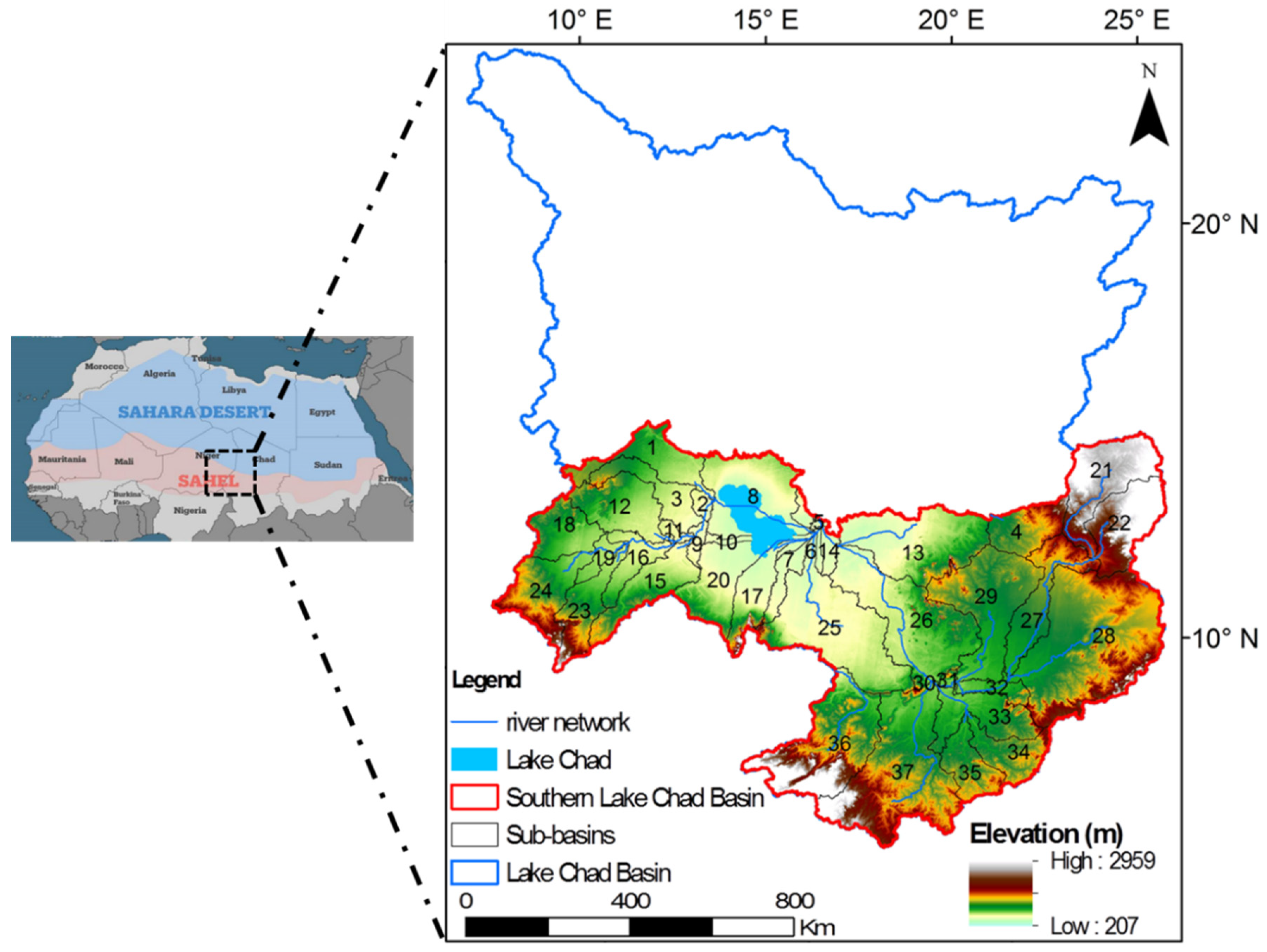
2.1. Study Area
2.2. Data
2.2.1. Forcing Data
Atmospheric Forcing Data
Precipitation
2.2.2. Remote Sensing ETa Data
2.2.3. Soil Moisture
2.2.4. Total Water Storage Change
2.2.5. Auxiliary Data
3. Methodology
3.1. Model Description
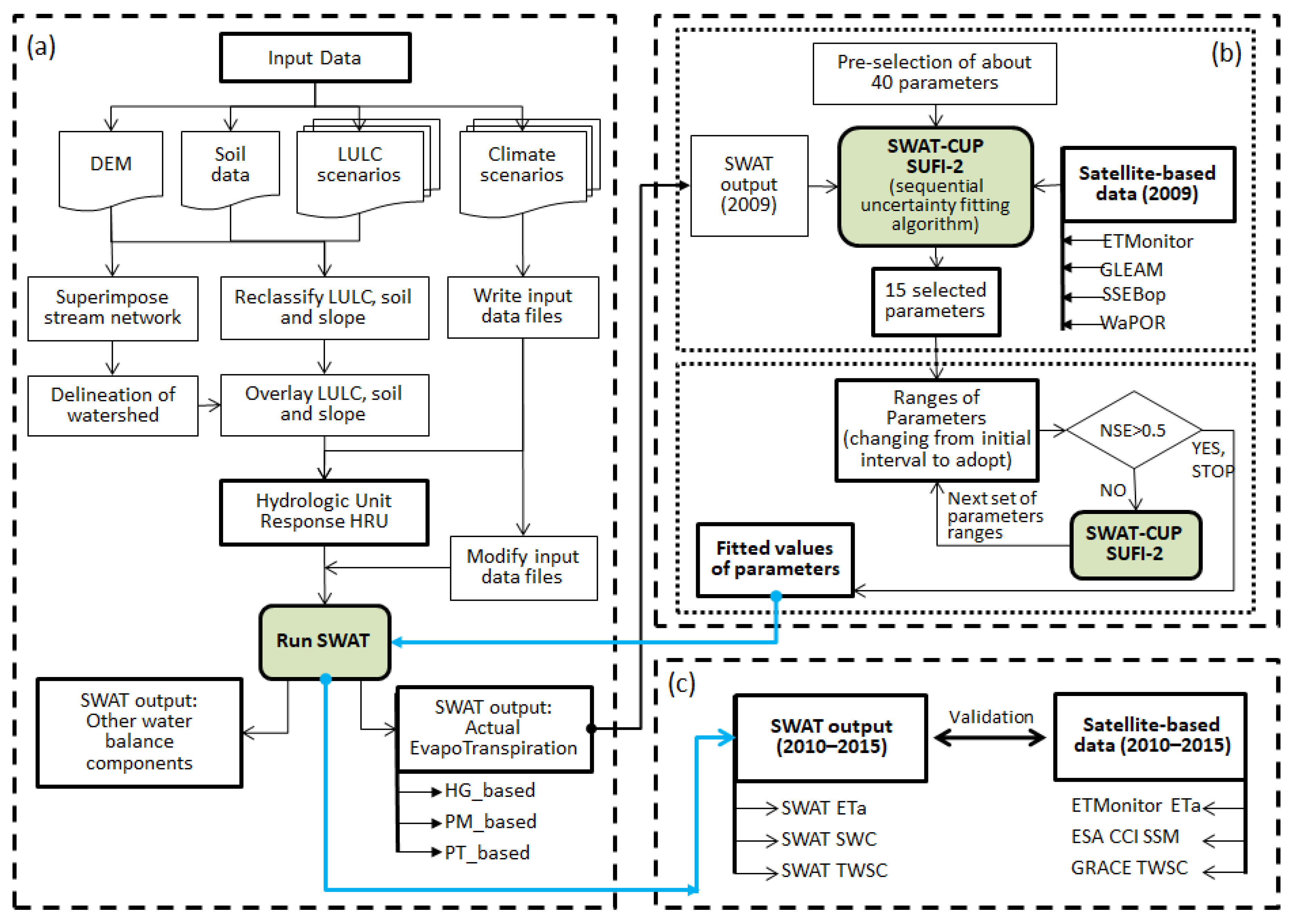
3.2. Model Setup
3.3. Calibration Procedure
3.4. Evaluation of Calibration, Validation, and Uncertainty Analysis
4. Results
4.1. Sensitivity Study
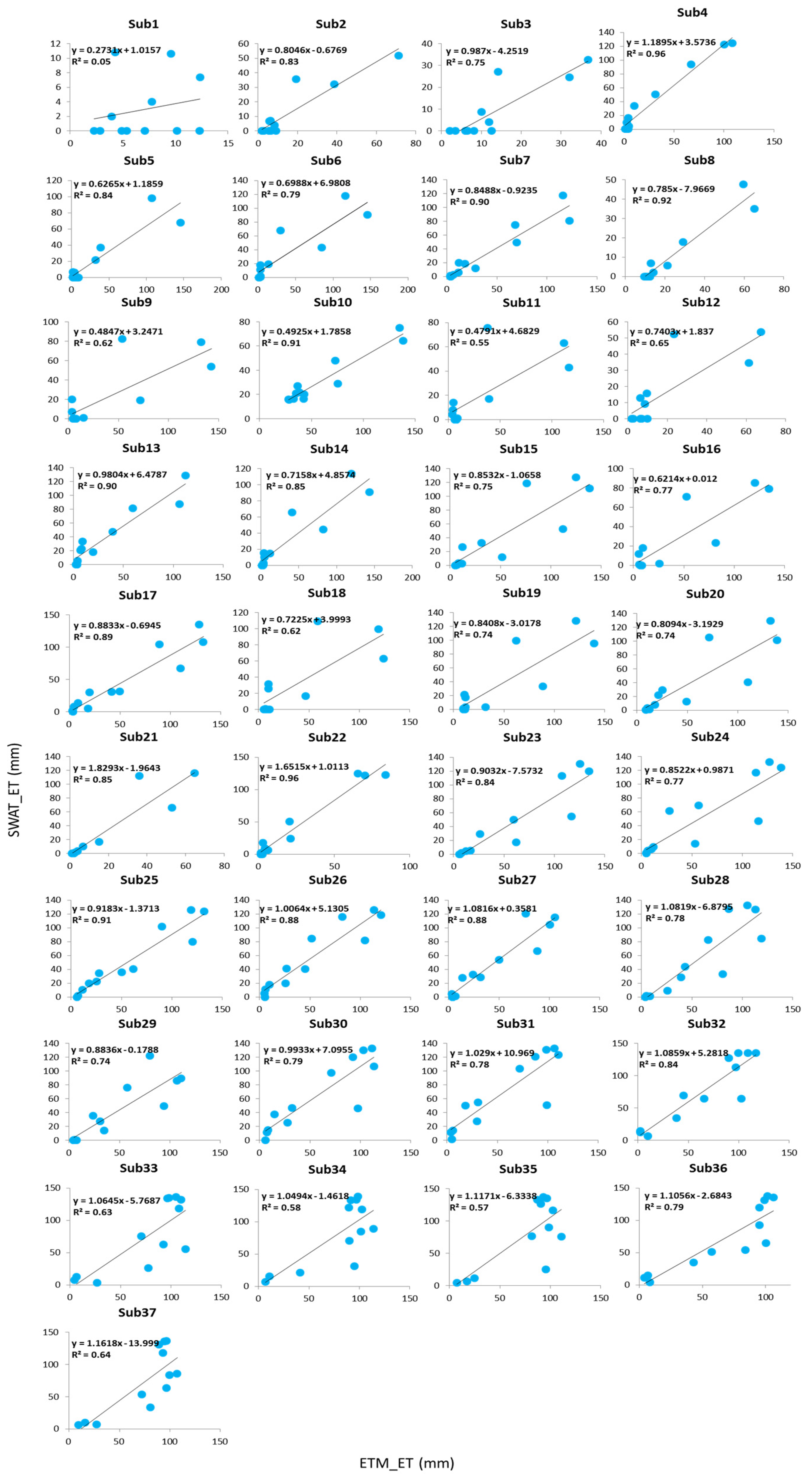
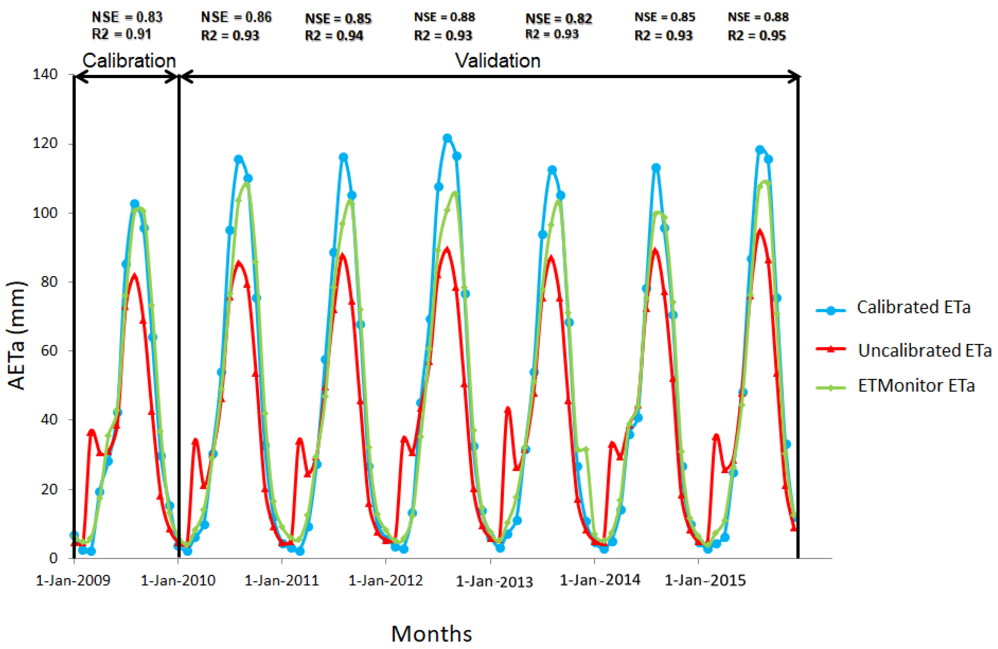
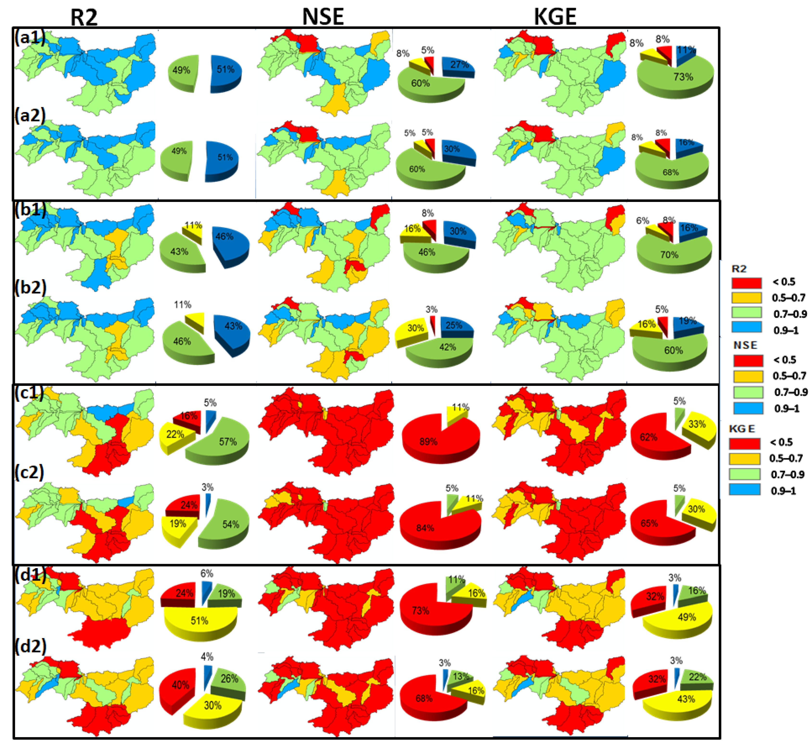
4.2. Calibration Results
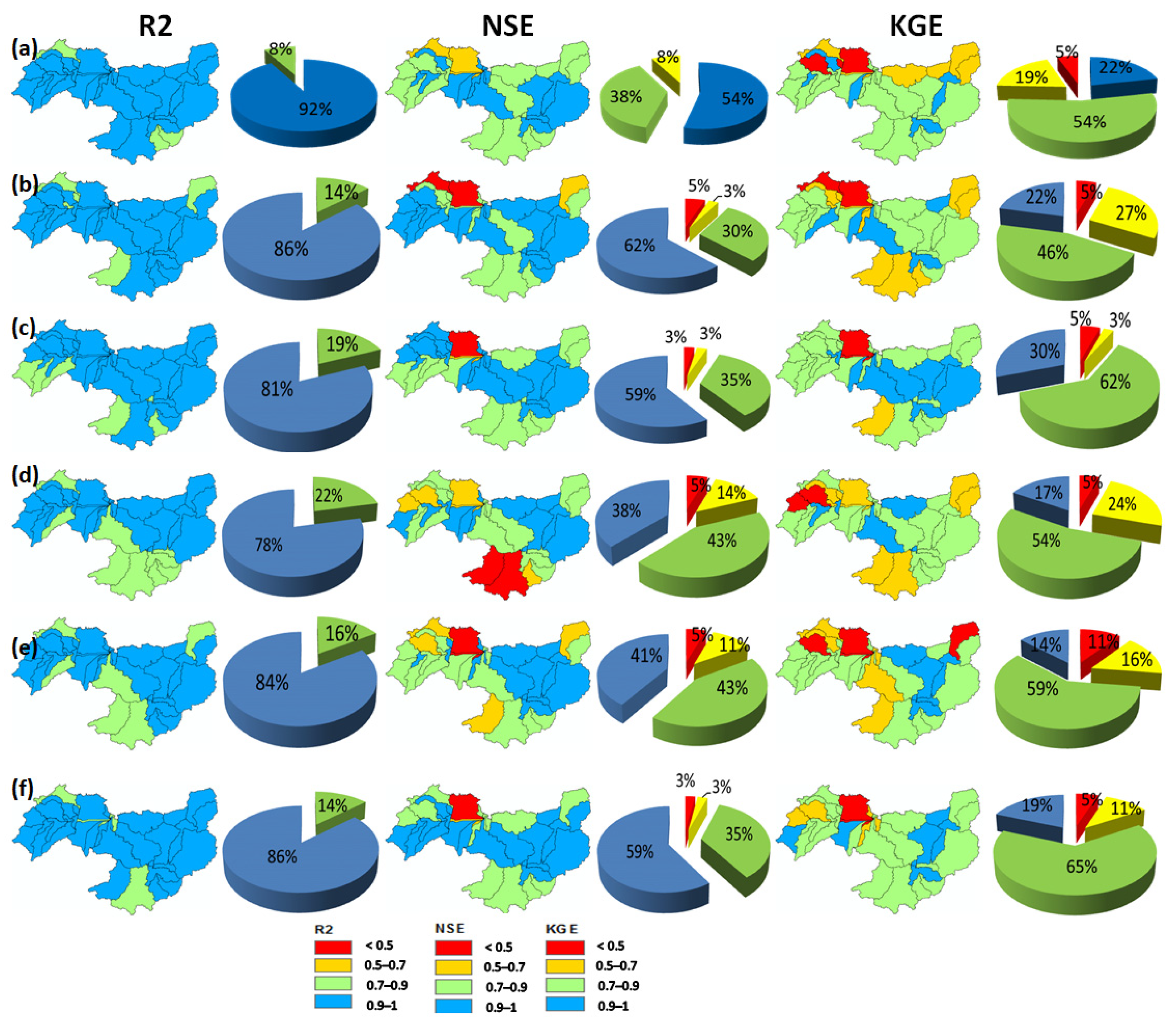
4.3. Validation Results
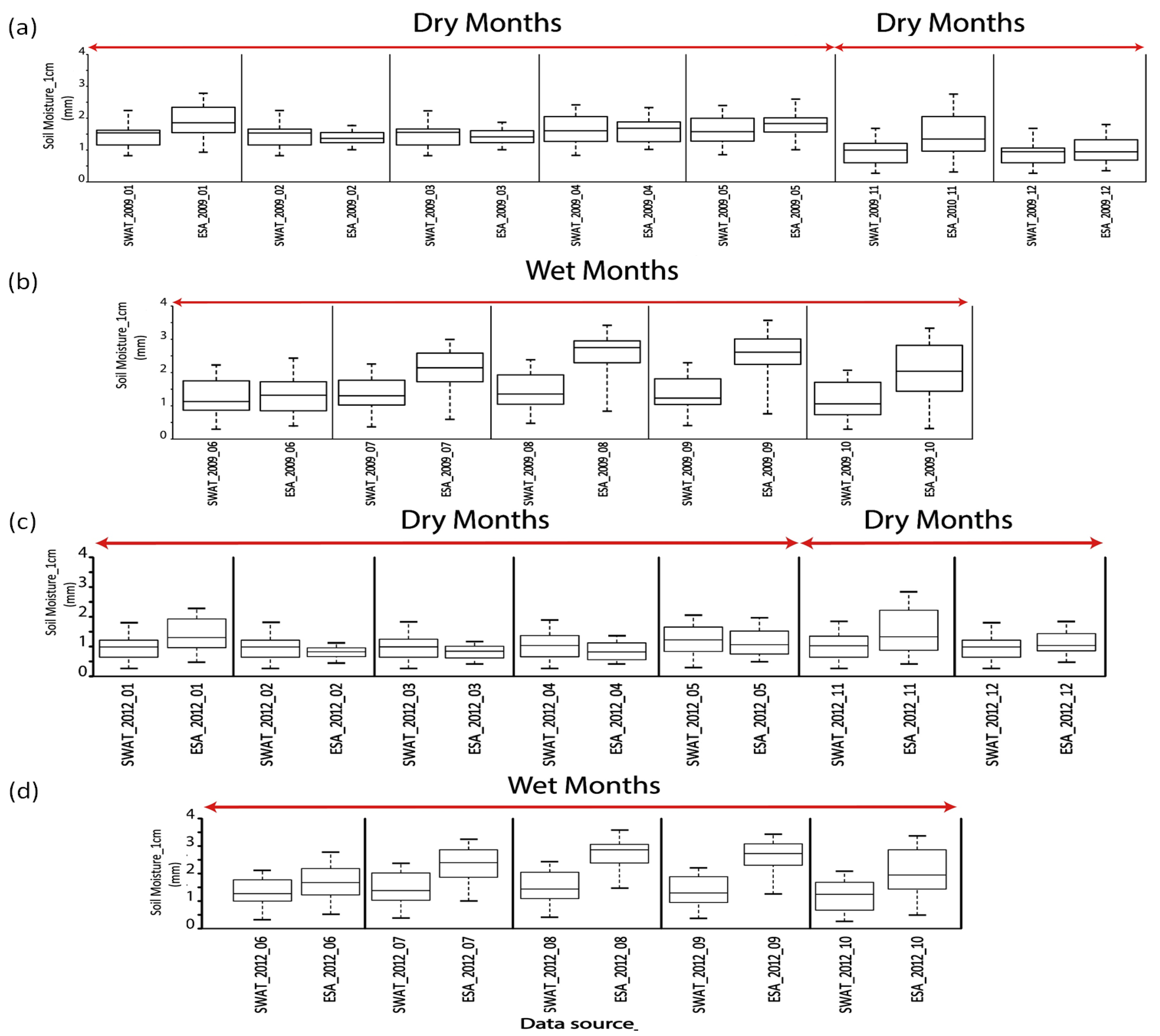
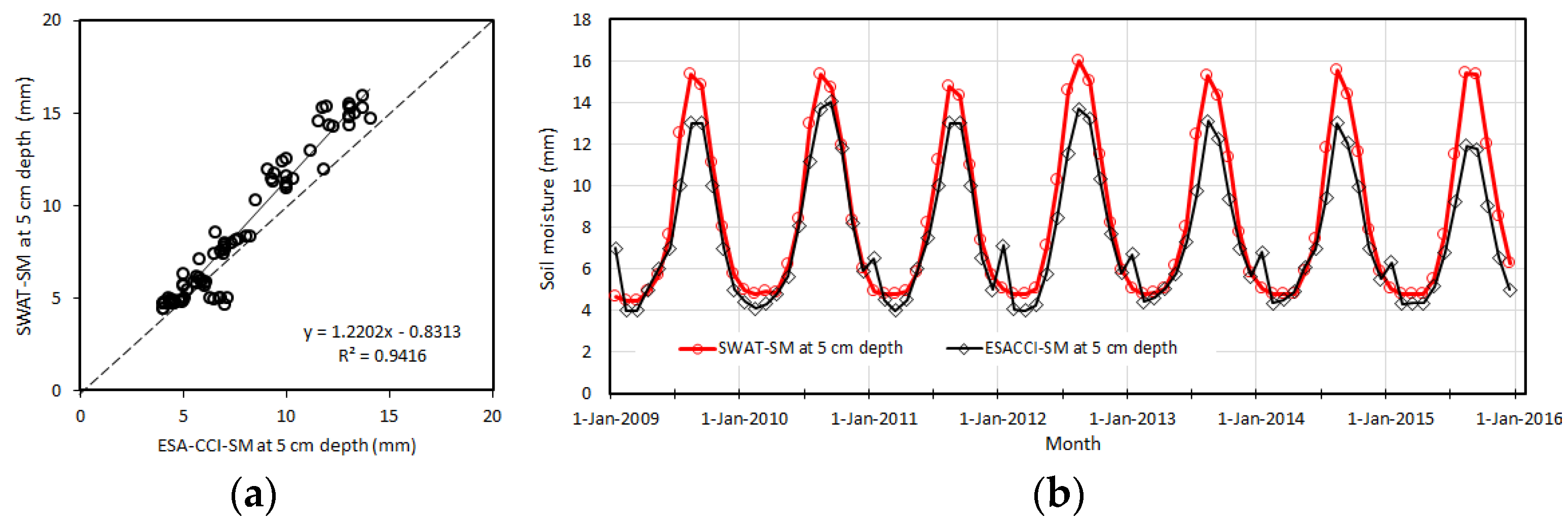
4.3.1. Validation of SWAT Soil Moisture
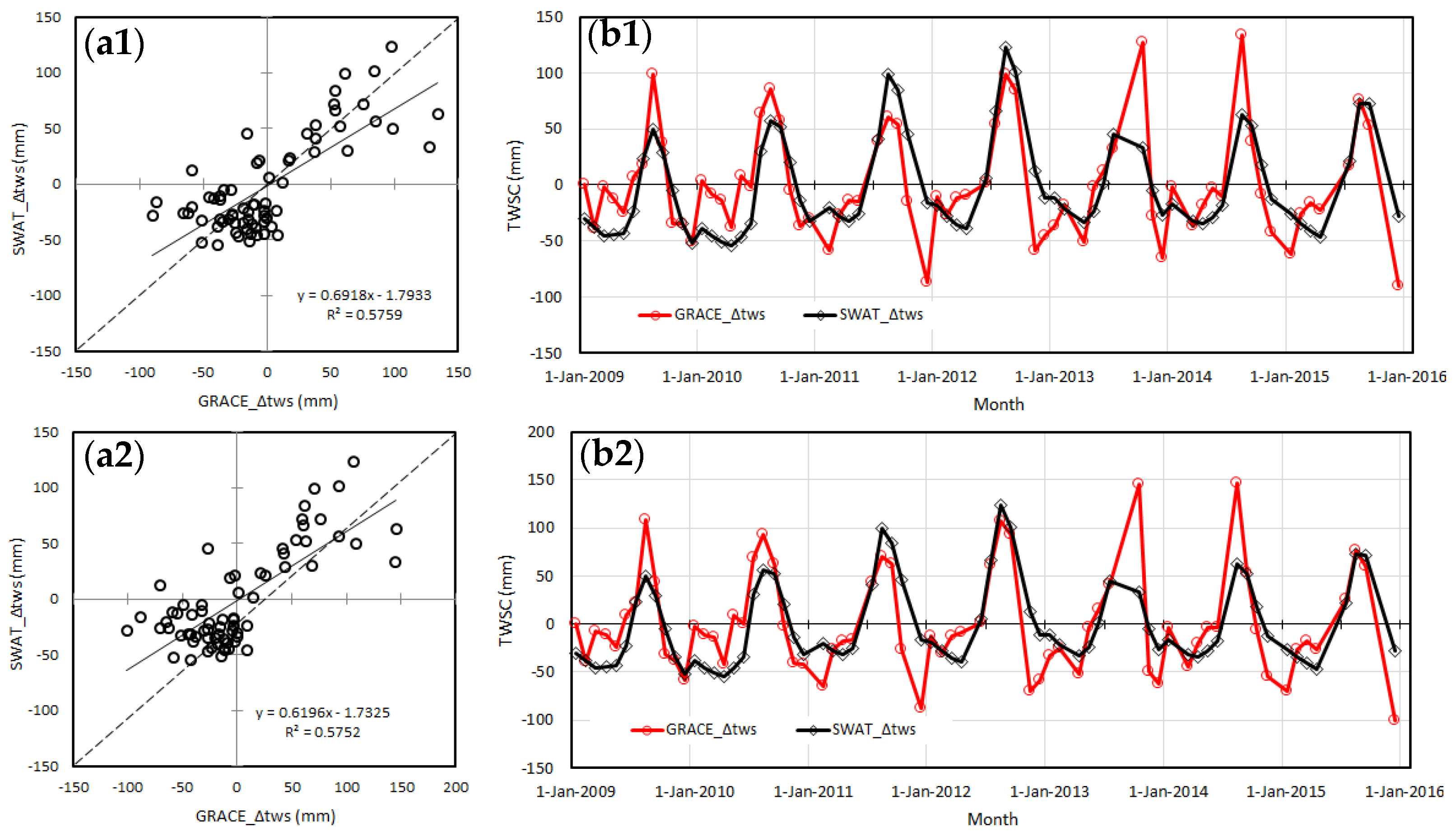
4.3.2. Validation of SWAT Estimates of Changes in Total Water Storage
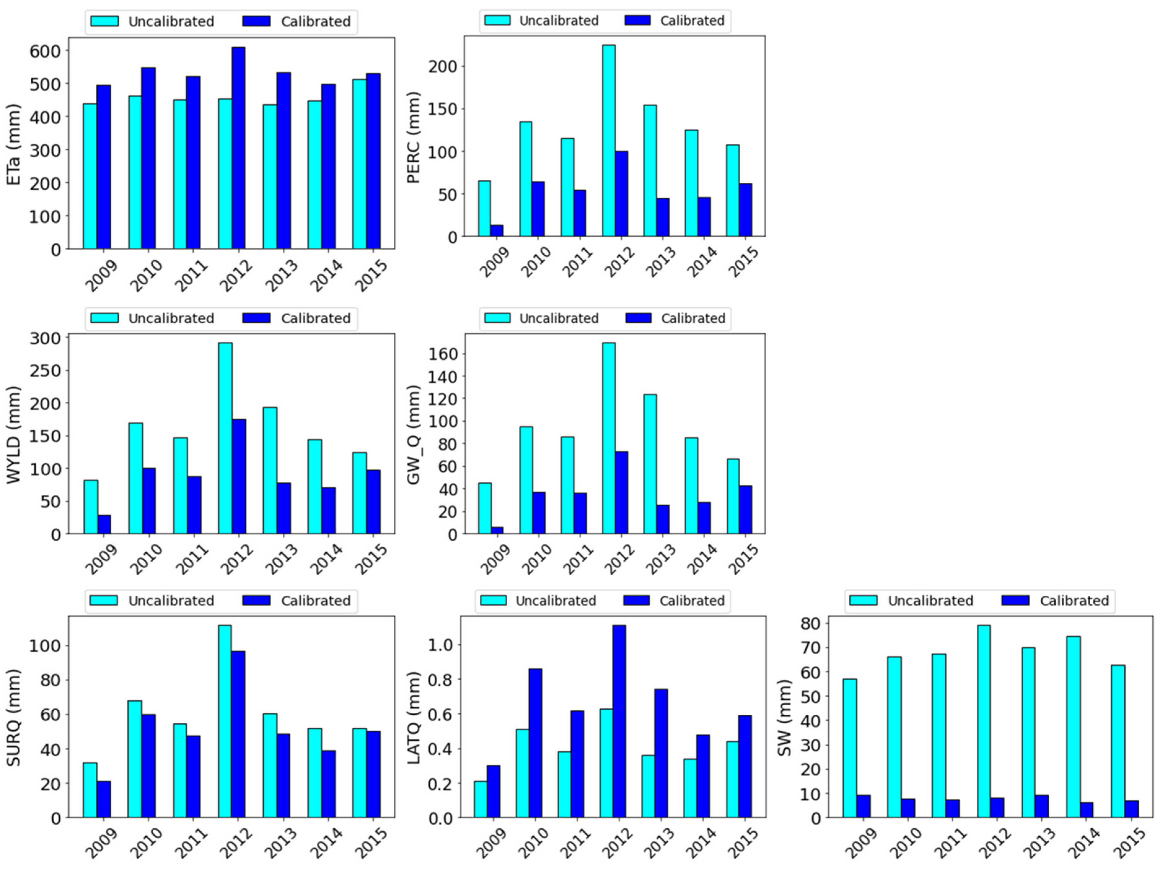
4.4. Water Balance
5. Discussion
6. Conclusions
Author Contributions
Funding
Data Availability Statement
Conflicts of Interest
Appendix A

| Parameters | Fitted Values | |||||||||||
|---|---|---|---|---|---|---|---|---|---|---|---|---|
| ETMonitor | WaPOR | SSEBop | GLEAM | |||||||||
| 1 * | 2 * | 3 * | 4 * | 5 * | 6 * | 7 * | 8 * | 9 * | 10 * | 11 * | 12 * | |
| r__CN2.mgt | 0.02 | 0.00 | −0.12 | −0.04 | −0.01 | −0.15 | −0.12 | 0.01 | 0.09 | 0.09 | 0.12 | 0.08 |
| r__SOL_AWC.sol | 0.94 | 0.79 | 0.84 | 0.94 | 0.97 | 0.94 | 0.95 | 0.92 | 0.95 | 0.94 | 0.90 | 0.56 |
| r__SOL_BD.sol | −0.11 | −0.30 | −0.26 | −0.43 | 0.13 | −0.03 | −0.49 | −0.02 | −0.01 | −0.07 | 0.09 | −0.10 |
| r__SOL_ALB.sol | 0.18 | 0.06 | 0.04 | 0.04 | 0.13 | 0.04 | −0.01 | −0.02 | 0.06 | 0.06 | 0.06 | 0.19 |
| v__ESCO.hru | 0.34 | 0.69 | 0.45 | 0.91 | 0.92 | 0.90 | 0.93 | 0.95 | 1.00 | 0.81 | 0.82 | 0.90 |
| v__BLAI{15,16}.plant | 3.39 | 0.51 | 3.43 | 4.95 | 4.60 | 3.04 | 4.90 | 4.43 | 3.96 | 1.56 | 1.30 | 4.87 |
| v__GSI{15,16}.plant | 1.73 | 1.64 | 0.01 | 1.38 | 4.86 | 0.10 | 1.03 | 1.05 | 0.07 | 1.72 | 1.76 | 0.00 |
| r__HRU_SLP.hru | 0.09 | 0.07 | 0.11 | 0.16 | 0.16 | 0.16 | 0.18 | 0.17 | 0.17 | 0.08 | 0.08 | 0.00 |
| r__SOL_CBN.sol | 0.10 | 0.15 | 0.12 | 0.14 | 0.03 | 0.11 | 0.14 | 0.14 | 0.11 | −0.01 | 0.03 | 0.11 |
| r__SOL_Z.sol | 0.20 | 0.19 | 0.18 | 0.17 | 0.19 | 0.17 | 0.13 | 0.14 | 0.17 | 0.20 | 0.16 | 0.20 |
| v__SLSOIL.hru | 103.74 | 138.64 | 67.12 | 123.67 | 100.54 | 104.30 | 118.26 | 116.20 | 146.00 | 126.21 | 140.98 | 66.22 |
| v__FFCB.bsn | 0.54 | 0.93 | 0.88 | 0.61 | 0.88 | 0.86 | 0.46 | 0.25 | 0.58 | 0.73 | 0.63 | 0.98 |
| v__DDRAIN.mgt | 140.34 | 122.43 | 178.44 | 153.39 | 106.34 | 157.98 | 118.14 | 116.34 | 138.64 | 139.21 | 108.2 | 144.75 |
| v__EPCO.hru | 0.72 | 0.06 | 0.37 | 0.43 | 0.59 | 0.34 | 0.46 | 0.60 | 0.30 | 0.11 | 0.17 | 0.06 |
| v__SURLAG.bsn | 9.22 | 9.17 | 2.34 | 4.02 | 6.74 | 9.34 | 5.55 | 7.28 | 2.84 | 8.49 | 9.75 | 1.80 |


References
- Chen, C.; Park, T.; Wang, X.; Piao, S.; Xu, B.; Chaturvedi, R.K.; Fuchs, R.; Brovkin, V.; Ciais, P.; Fensholt, R.; et al. China and India lead in greening of the world through land-use management. Nat. Sustain. 2019, 2, 122–129. [Google Scholar] [CrossRef] [PubMed]
- Odada, E.O.; Oyebande, L.; Oguntola, A.J. Lake Chad: Experience and lessons learned Brief. In Proceedings of the International Lake Environment Committee Foundation, Kusatsu, Japan, 27 November 2006; pp. 75–91. [Google Scholar]
- Carroll, S.; Liu, A.; Dawes, L.; Hargreaves, M.; Goonetilleke, A. Role of Land Use and Seasonal Factors in Water Quality Degradations. Water Resour. Manag. 2013, 27, 3433–3440. [Google Scholar] [CrossRef] [Green Version]
- McDonald, R.I.; Weber, K.; Padowski, J.; Flörke, M.; Schneider, C.; Green, P.A.; Gleeson, T.; Eckman, S.; Lehner, B.; Balk, D.; et al. Water on an urban planet: Urbanization and the reach of urban water infrastructure. Glob. Environ. Chang. 2014, 27, 96–105. [Google Scholar] [CrossRef] [Green Version]
- Arnold, J.G.; Srinivasan, R.; Muttiah, R.S.; Williams, J.R. Large area hydrologic modeling and assessment part I: Model development. J. Am. Water Resour. Assoc. 1998, 34, 73–89. [Google Scholar] [CrossRef]
- Awotwi, A.; Kumi, M.; Jansson, P.E.; Yeboah, F.; Nti, I.K. Predicting Hydrological Response to Climate Change in the White Volta Catchment, West Africa. J. Earth Sci. Clim. Chang. 2015, 6, 249. [Google Scholar] [CrossRef]
- Cheng, Y.; He, H.; Cheng, N.; He, W. The Effects of Climate and Anthropogenic Activity on Hydrologic Features in Yanhe River. Adv. Meteorol. 2016, 2016, 5297158. [Google Scholar] [CrossRef] [Green Version]
- Schuol, J.; Abbaspour, K.C. Calibration and uncertainty issues of a hydrological model ( SWAT ) applied to West Africa. Adv. Geosci. 2006, 9, 137–143. [Google Scholar] [CrossRef] [Green Version]
- Laurent, F.; Ruelland, D. Modélisation à base physique de la variabilité hydroclimatique à l’échelle d’un grand bassin versant tropical. In Global Change: Facing Risks and Threats to Water Resour; Fez: Morroco, France, 2010; pp. 474–484. [Google Scholar]
- Adeogun, A.; Sule, B.; Salami, A.; Okeola, O. GIS-Based Hydrological Modelling Using Swat: Case Study of Upstream Watershed of Jebba Reservoir in Nigeria. Niger. J. Technol. 2014, 33, 351. [Google Scholar] [CrossRef]
- Nkiaka, E.; Nawaz, N.R.; Lovett, J.C. Effect of single and multi-site calibration techniques on hydrological model performance, parameter estimation and predictive uncertainty: A case study in the Logone catchment, Lake Chad basin. Stoch. Environ. Res. Risk Assess. 2018, 32, 1665–1682. [Google Scholar] [CrossRef] [Green Version]
- Schuol, J.; Abbaspour, K.C.; Srinivasan, R.; Yang, H. Estimation of freshwater availability in the West African sub-continent using the SWAT hydrologic model. J. Hydrol. 2007, 352, 30–49. [Google Scholar] [CrossRef]
- Mengistu, A.G.; van Rensburg, L.D.; Woyessa, Y.E. Techniques for calibration and validation of SWAT model in data scarce arid and semi-arid catchments in South Africa. J. Hydrol. Reg. Stud. 2019, 25, 100621. [Google Scholar] [CrossRef]
- Senay, G.; Leake, S.; Nagler, P.L.; Artan, G.; Dickinson, J.; Cordova, J.; Glenn, E. Estimating basin scale evapotranspiration (ET) by water balance and remote sensing methods. Hydrol. Process. 2011, 25, 4037–4049. [Google Scholar] [CrossRef]
- Zheng, C.; Jia, L.; Hu, G.; Lu, J.; Wang, K.; Li, Z. Global evapotranspiration derived by ETMonitor model based on earth observations. Int. Geosci. Remote Sens. Symp. 2016, 2016, 222–225. [Google Scholar] [CrossRef]
- Martens, B.; Miralles, D.G.; Lievens, H.; Van Der Schalie, R.; De Jeu, R.A.M.; Fernández-Prieto, D.; Beck, H.E.; Dorigo, W.A.; Verhoest, N.E.C. GLEAM v3: Satellite-based land evaporation and root-zone soil moisture. Geosci. Model Dev. 2017, 10, 1903–1925. [Google Scholar] [CrossRef] [Green Version]
- Miralles, D.G.; Holmes, T.R.H.; De Jeu, R.A.M.; Gash, J.H.; Meesters, A.G.C.A.; Dolman, A.J. Global land-surface evaporation estimated from satellite-based observations. Hydrol. Earth Syst. Sci. 2011, 15, 453–469. [Google Scholar] [CrossRef] [Green Version]
- Lopez Lopez, P.; Sutanudjaja, E.; Schellekens, J.; Sterk, G.; Bierkens, M. Calibration of a large-scale hydrological model using satellite-based soil moisture and evapotranspiration products. Hydrol. Earth Syst. Sci. 2017, 21, 3125–3144. [Google Scholar] [CrossRef] [Green Version]
- Ha, L.T.; Bastiaanssen, W.G.M.; van Griensven, A.; van Dijk, A.I.J.M.; Senay, G.B. Calibration of spatially distributed hydrological processes and model parameters in SWAT using remote sensing data and an auto-calibration procedure: A case study in a Vietnamese river basin. Water 2018, 10, 212. [Google Scholar] [CrossRef] [Green Version]
- Poméon, T.; Diekkrüger, B.; Springer, A.; Kusche, J.; Eicker, A. Multi-objective validation of SWAT for sparsely-gaugedWest African river basins—A remote sensing approach. Water 2018, 10, 451. [Google Scholar] [CrossRef] [Green Version]
- Odusanya, A.E.; Mehdi, B.; Schürz, C.; Oke, A.O.; Awokola, O.S.; Awomeso, J.A.; Adejuwon, J.O.; Schulz, K. Multi-site calibration and validation of SWAT with satellite-based evapotranspiration in a data-sparse catchment in southwestern Nigeria. Hydrol. Earth Syst. Sci. 2019, 23, 1113–1144. [Google Scholar] [CrossRef] [Green Version]
- Tang, L.; Yang, D.; Hu, H.; Gao, B. Detecting the effect of land-use change on streamflow, sediment and nutrient losses by distributed hydrological simulation. J. Hydrol. 2011, 409, 172–182. [Google Scholar] [CrossRef]
- Coe, M.T.; Foley, J.A. Human and natural impacts on the water resources of the Lake Chad basin. J. Geophys. Res. Atmos. 2001, 106, 3349–3356. [Google Scholar] [CrossRef]
- Gao, H.; Bohn, T.J.; Podest, E.; McDonald, K.C.; Lettenmaier, D.P. On the causes of the shrinking of Lake Chad. Environ. Res. Lett. 2011, 6. [Google Scholar] [CrossRef] [Green Version]
- Zhu, W.; Yan, J.; Jia, S. Monitoring recent fluctuations of the southern pool of lake chad using multiple remote sensing data: Implications for water balance analysis. Remote Sens. 2017, 9, 1032. [Google Scholar] [CrossRef] [Green Version]
- Policelli, F.; Hubbard, A.; Jung, H.C.; Zaitchik, B.; Ichoku, C. A predictive model for Lake Chad total surface water area using remotely sensed and modeled hydrological and meteorological parameters and multivariate regression analysis. J. Hydrol. 2019, 568, 1071–1080. [Google Scholar] [CrossRef]
- Lemoalle, J.; Magrin, G. Development of Lake Chad Current Situation and Posiible Outcomes, IRD ed.; Robert, S., André, L.V., Eds.; OpenEdition Books: Marseille, France, 2014; ISBN 9782709918367. [Google Scholar]
- Frenken, K.; Jean-Marc, F. Irrigation Potential in Africa: A Basin Approach; FAO: Rome, Italy, 1997; ISBN 92-5-103966-6. [Google Scholar]
- Policelli, F.; Hubbard, A.; Jung, H.C.; Zaitchik, B.; Ichoku, C. Lake Chad total surface water area as derived from Land Surface Temperature and radar remote sensing data. Remote Sens. 2018, 10, 252. [Google Scholar] [CrossRef] [Green Version]
- Mahamat Nour, A.; Vallet-Coulomb, C.; Gonçalves, J.; Sylvestre, F.; Deschamps, P. Rainfall-discharge relationship and water balance over the past 60 years within the Chari-Logone sub-basins, Lake Chad basin. J. Hydrol. Reg. Stud. 2021, 35, 100824. [Google Scholar] [CrossRef]
- Delclaux, F.; Le Coz, M.; Coe, M.; Favreau, G.; Ngounou Ngatcha, B. Confronting Models with Observations for Evaluating Hydrological Change in the Lake Chad Basin, Africa. In Proceedings of the 13th IWRA World Water Congress, Montpellier, France, 1–4 September 2008. [Google Scholar]
- Hersbach, H.; Bell, B.; Berrisford, P.; Hirahara, S.; Horányi, A.; Muñoz-Sabater, J.; Nicolas, J.; Peubey, C.; Radu, R.; Schepers, D.; et al. The ERA5 global reanalysis. Q. J. R. Meteorol. Soc. 2020, 146, 1999–2049. [Google Scholar] [CrossRef]
- Funk, C.; Peterson, P.; Landsfeld, M.; Pedreros, D.; Verdin, J.; Shukla, S.; Husak, G.; Rowland, J.; Harrison, L.; Hoell, A.; et al. The climate hazards infrared precipitation with stations—A new environmental record for monitoring extremes. Sci. Data 2015, 2, 150066. [Google Scholar] [CrossRef] [Green Version]
- Katsanos, D.; Retalis, A.; Michaelides, S. Validation of a high-resolution precipitation database (CHIRPS) over Cyprus for a 30-year period. Atmos. Res. 2016, 169, 459–464. [Google Scholar] [CrossRef]
- Wang, J.; Zhao, Y.; Li, C.; Yu, L.; Liu, D.; Gong, P. Mapping global land cover in 2001 and 2010 with spatial-temporal consistency at 250m resolution. ISPRS J. Photogramm. Remote Sens. 2015, 103, 38–47. [Google Scholar] [CrossRef]
- Jia, L.; Zheng, C.; Hu, G.C.; Menenti, M. Evapotranspiration. In Comprehensive Remote Sensing; Elsevier: Beijing, China, 2018; Volumes 1–9, pp. 25–50. ISBN 9780128032206. [Google Scholar]
- Senay, G.B.; Bohms, S.; Singh, R.K.; Gowda, P.H.; Velpuri, N.M.; Alemu, H.; Verdin, J.P. Operational Evapotranspiration Mapping Using Remote Sensing and Weather Datasets: A New Parameterization for the SSEB Approach. J. Am. Water Resour. Assoc. 2013, 49, 577–591. [Google Scholar] [CrossRef] [Green Version]
- WaPOR Database Methodology: Level 1 Remote Sensing for Water Productivity Technical Report: Methodology Series; FAO: Rome, Italy, 2018; ISBN 978-92-5-109769-4.
- Gruber, A.; Dorigo, W.A.; Crow, W.; Wagner, W. Triple Collocation-Based Merging of Satellite Soil Moisture Retrievals. IEEE Trans. Geosci. Remote Sens. 2017, 55, 6780–6792. [Google Scholar] [CrossRef]
- Gruber, A.; Scanlon, T.; Van Der Schalie, R.; Wagner, W.; Dorigo, W. Evolution of the ESA CCI Soil Moisture climate data records and their underlying merging methodology. Earth Syst. Sci. Data 2019, 11, 717–739. [Google Scholar] [CrossRef] [Green Version]
- Dorigo, W.; Wagner, W.; Albergel, C.; Albrecht, F.; Balsamo, G.; Brocca, L.; Chung, D.; Ertl, M.; Forkel, M.; Gruber, A.; et al. ESA CCI Soil Moisture for improved Earth system understanding: State-of-the art and future directions. Remote Sens. Environ. 2017, 203, 185–215. [Google Scholar] [CrossRef]
- Tapley, B.D.; Bettadpur, S.; Watkins, M.; Reigber, C. The gravity recovery and climate experiment: Mission overview and early results. Geophys. Res. Lett. 2004, 31, 1–4. [Google Scholar] [CrossRef] [Green Version]
- Wahr, J.; Molenaar, M.; Bryan, F. Time variability of the Earth’s gravity field: Hydrological and oceanic effects and their possible detection using GRACE. J. Geophys. Res. Solid Earth 1998, 103, 30205–30229. [Google Scholar] [CrossRef]
- Wouters, B.; Bonin, J.A.; Chambers, D.P.; Riva, R.E.M.; Sasgen, I.; Wahr, J. GRACE, time-varying gravity, Earth system dynamics and climate change. Rep. Prog. Phys. 2014, 77. [Google Scholar] [CrossRef] [Green Version]
- Save, H.; Bettadpur, S.; Tapley, B.D. High-resolution CSR GRACE RL05 mascons. J. Geophys. Res. Solid Earth 2016, 121, 7547–7569. [Google Scholar] [CrossRef]
- Biancamaria, S.; Mballo, M.; Le Moigne, P.; Sánchez Pérez, J.M.; Espitalier-Noël, G.; Grusson, Y.; Cakir, R.; Häfliger, V.; Barathieu, F.; Trasmonte, M.; et al. Total water storage variability from GRACE mission and hydrological models for a 50,000 km2 temperate watershed: The Garonne River basin (France). J. Hydrol. Reg. Stud. 2019, 24, 100609. [Google Scholar] [CrossRef]
- Long, D.; Longuevergne, L.; Scanlon, B.R. Uncertainty in evapotranspiration from land surface modeling, remote sensing, and GRACE satellites. Water Resour. Res. 2014, 50, 1131–1151. [Google Scholar] [CrossRef] [Green Version]
- George, C.; Leon, L.F. WaterBase: SWAT in an Open Source GIS. Open Hydrol. J. 2008, 2, 1–6. [Google Scholar] [CrossRef] [Green Version]
- Neitsch, S.L.; Arnold, J.G.; Kiniry, J.R.; Williams, J.R. Soil & Water Assessment Tool Theoretical Documentation Version 2009; Texas Water Resources Institute: College Station, TX, USA, 2011. [Google Scholar]
- Neitsch, S.L.; Arnold, J.G.; Kiniry, J.R. Soil and Water Assessment Tool Input/Output File Documentation Version 2009; Soil and Water Assessment Tool: College Station, TX, USA, 2011; p. 643. [Google Scholar]
- Neitsch, S.L.; Arnold, J.G.; Kiniry, J.R.; Williams, J.R. Soil and Water Assessment Tool Documentation Version 2005; Grassland, Soil and Water Research Laboratory: College Station, TX, USA, 2005; p. 476. [Google Scholar]
- Teshager, A.D.; Gassman, W.P.; Secchi, S.; Justin, T.S.; Girmaye, M. Modeling Agricultural Watersheds with the Soil and Water Assessment Tool (SWAT): Calibration and Validation with a Novel Procedure for Spatially Explicit HRUs. Environ. Manag. 2016, 57, 894–911. [Google Scholar] [CrossRef] [PubMed] [Green Version]
- Her, Y.; Frankenberger, J.; Chaubey, I.; Srinivasan, R. Threshold effects in HRU definition of the soil and water assessment tool. Am. Soc. Agric. Biol. Eng. 2015, 58, 367–378. [Google Scholar] [CrossRef]
- Abbaspour, K.C.; Rouholahnejad, E.; Vaghefi, S.; Srinivasan, R.; Yang, H.; Kløve, B. A continental-scale hydrology and water quality model for Europe: Calibration and uncertainty of a high-resolution large-scale SWAT model. J. Hydrol. 2015, 524, 733–752. [Google Scholar] [CrossRef] [Green Version]
- Abbaspour, K.C.; Johnson, C.A.; van Genuchten, M.T. Estimating Uncertain Flow and Transport Parameters Using a Sequential Uncertainty Fitting Procedure. Vadose Zone J. 2004, 3, 1340–1352. [Google Scholar] [CrossRef]
- Wang, X.; Melesse, A.M.; Yang, W. Influences of potential evapotranspiration estimation methods on SWAT’s hydrologic simulation in a northwestern Minnesota watershed. Trans. ASABE 2006, 49, 1755–1771. [Google Scholar] [CrossRef]
- Emam, A.R.; Kappas, M.; Linh, N.H.K.; Renchin, T. Hydrological modeling and runoff mitigation in an ungauged basin of central Vietnam using SWAT model. Hydrology 2017, 4, 16. [Google Scholar] [CrossRef] [Green Version]
- Boulain, N.; Cappelaere, B.; Séguis, L.; Favreau, G.; Gignoux, J. Water balance and vegetation change in the Sahel: A case study at the watershed scale with an eco-hydrological model. J. Arid Environ. 2009, 73, 1125–1135. [Google Scholar] [CrossRef]
- Moriasi, D.N.; Gitau, M.W.; Pai, N.; Daggupati, P. Hydrologic and water quality models: Performance measures and evaluation criteria. Am. Soc. Agric. Biol. Eng. 2015, 58, 1763–1785. [Google Scholar] [CrossRef] [Green Version]
- Moriasi, D.N.; Arnold, J.G.; Van Liew, M.W.; Bingner, R.L.; Harmel, R.D.; Veith, T.L. Model evaluation guidelines for systematic quantification of accuracy in watershed simulations. Am. Soc. Agric. Biol. Eng. 2007, 50, 885–900. [Google Scholar] [CrossRef]
- Abbaspour, K.C. SWAT-CUP SWAT Calibration and Uncertainty Programs—A User Manual 2015; Swiss Federal Institute of Aqualtic Science and Technology: Dübendorf, Switzerland, 2015. [Google Scholar]
- Schuol, J.; Abbaspour, K.C. Using monthly weather statistics to generate daily data in a SWAT model application to West Africa. Ecol. Model. 2007, 201, 301–311. [Google Scholar] [CrossRef]
- Djaman, K.; Tabari, H.; Balde, A.B.; Diop, L.; Futakuchi, K.; Irmak, S. Analyses, calibration and validation of evapotranspiration models to predict grass-reference evapotranspiration in the Senegal river delta. J. Hydrol. Reg. Stud. 2016, 8, 82–94. [Google Scholar] [CrossRef] [Green Version]
- Samadi, S.Z. Assessing the sensitivity of SWAT physical parameters to potential evapotranspiration estimation methods over a coastal plain watershed in the southeastern United States. Hydrol. Res. 2017, 48, 395–415. [Google Scholar] [CrossRef]
- Nash, J.E.; Sutcliffe, J.V. River flow forecasting through conceptual models Part I—A discussion of principales. J. Hydrol. 1970, 10, 282–290. [Google Scholar] [CrossRef]
- Gupta, H.V.; Kling, H.; Yilmaz, K.K.; Martinez, G.F. Decomposition of the mean squared error and NSE performance criteria: Implications for improving hydrological modelling. J. Hydrol. 2009, 377, 80–91. [Google Scholar] [CrossRef] [Green Version]
- Gupta, H.V.; Sorooshian, S.; Yapo, P.O. Status of Automatic Calibration for Hydrologic Models: Comparison with Multilevel Expert Calibration. J. Hydrol. Eng. 1999, 4, 135–143. [Google Scholar] [CrossRef]
- Rajib, M.A.; Merwade, V.; Yu, Z. Multi-objective calibration of a hydrologic model using spatially distributed remotely sensed/in-situ soil moisture. J. Hydrol. 2016, 536, 192–207. [Google Scholar] [CrossRef] [Green Version]
- Rodell, M.; Famiglietti, J.S. Detectability of variations in continental water storage from satellite observations of the time dependent gravity field. Water Resour. Res. 1999, 35, 2705–2723. [Google Scholar] [CrossRef] [Green Version]
- Kouchi, D.H.; Esmaili, K.; Faridhosseini, A.; Sanaeinejad, S.H.; Khalili, D.; Abbaspour, K.C. Sensitivity of calibrated parameters and water resource estimates on different objective functions and optimization algorithms. Water 2017, 9, 384. [Google Scholar] [CrossRef] [Green Version]
- Weerasinghe, I.; Bastiaanssen, W.; Mul, M.; Jia, L.; Van Griensven, A. Can we trust remote sensing evapotranspiration products over Africa. Hydrol. Earth Syst. Sci. 2020, 24, 1565–1586. [Google Scholar] [CrossRef] [Green Version]
- Trambauer, P.; Dutra, E.; Maskey, S.; Werner, M.; Pappenberger, F.; Van Beek, L.P.H.; Uhlenbrook, S. Comparison of different evaporation estimates over the African continent. Hydrol. Earth Syst. Sci. 2014, 18, 193–212. [Google Scholar] [CrossRef] [Green Version]
- Grippa, M.; Kergoat, L.; Frappart, F.; Araud, Q.; Boone, A.; De Rosnay, P.; Lemoine, J.M.; Gascoin, S.; Balsamo, G.; Ottlé, C.; et al. Land water storage variability over West Africa estimated by Gravity Recovery and Climate Experiment (GRACE) and land surface models. Water Resour. Res. 2011, 47, 1–18. [Google Scholar] [CrossRef]
- Ndehedehe, C.; Awange, J.; Agutu, N.; Kuhn, M.; Heck, B. Understanding changes in terrestrial water storage over West Africa between 2002 and 2014. Adv. Water Resour. 2016, 88, 211–230. [Google Scholar] [CrossRef] [Green Version]
- Report on the State of the Lake Chad Basin Ecosystem; Lake Chad Basin Commission and German Cooperation: N’Djamena, Chad, 2016.
- Lemoalle, J.; Bader, J.C.; Leblanc, M.; Sedick, A. Recent changes in Lake Chad: Observations, simulations and management options (1973–2011). Glob. Planet. Chang. 2012, 80–81, 247–254. [Google Scholar] [CrossRef]
- Olivry, J.; Chouret, A.; Lemoalle, J.; Bricquet, J. Hydrologie du lac Tchad; ORSTOM: Paris, France, 1996; ISBN 2-7099-1353-4. [Google Scholar]
- Pham-Duc, B.; Sylvestre, F.; Papa, F.; Frappart, F.; Bouchez, C.; Crétaux, J.F. The Lake Chad hydrology under current climate change. Sci. Rep. 2020, 10, 5498. [Google Scholar] [CrossRef] [Green Version]
- Vuillaume, G. Bilan hydrologique mensuel et modelisation sommaire du regime hydrologique du lac Tchad. Cah. ORSTOM Hydrol. 1981, 18, 23–72. [Google Scholar]
- Mahmood, R.; Jia, S. Assessment of hydro-climatic trends and causes of dramatically declining stream flow to Lake Chad, Africa, using a hydrological approach. Sci. Total Environ. 2019, 675, 122–140. [Google Scholar] [CrossRef]
- Zhu, W.; Jia, S.; Lall, U.; Cao, Q.; Mahmood, R. Relative contribution of climate variability and human activities on the water loss of the Chari/Logone River discharge into Lake Chad: A conceptual and statistical approach. J. Hydrol. 2019, 569, 519–531. [Google Scholar] [CrossRef]
- Bastiaanssen, W.G.M.; Cheema, M.J.M.; Immerzeel, W.W.; Miltenburg, I.J.; Pelgrum, H. Surface energy balance and actual evapotranspiration of the transboundary Indus Basin estimated from satellite measurements and the ETLook model. Water Resour. Res. 2012, 48, 1–16. [Google Scholar] [CrossRef] [Green Version]
- Monteith, J.L. Evaporation and environment. Symp. Soc. Exp. Biol. 1965, 19, 205–234. [Google Scholar]
- Miralles, D.G.; De Jeu, R.A.M.; Gash, J.H.; Holmes, T.R.H.; Dolman, A.J. Magnitude and variability of land evaporation and its components at the global scale. Hydrol. Earth Syst. Sci. 2011, 15, 967–981. [Google Scholar] [CrossRef] [Green Version]


| Products | Temporal Coverage | Spatial Resolution | Source/Reference |
|---|---|---|---|
| DEM | 2000 | 30 m | Shuttle Radar Topography Mission (SRTM) 30 m Digital Elevation Data (www.earthexplorer.usgs.gov; accessed on 6 December 2019) |
| Soil | - | 1 km | Digital Soil Map of the World (DSMW) version 3.6: Land and Water Development Division, FAO, Rome |
| LULC | 2000–2019 | 250 m | [35] |
| Precipitation | 1981–2021 | 5 km | CHIRPS: https://data.chc.ucsb.edu/products/CHIRPS-2.0/global_daily/tifs/p05/; accessed on 24 June 2020 |
| Min/Max Temperature | 1950–2021 | ECMWF ERA5 [33] | |
| Wind speed | 31 km | ||
| Relative humidity | |||
| Solar radiation |
| Product | Temporal Coverage | Spatial Resolution | Estimation Approach | Input Data Source | Reference |
|---|---|---|---|---|---|
| ETMonitor | 2001–2020 Produced by co-author of this study | 1 km | P-M, Gash model, Shuttleworth–Wallace, calculates E, T, and I separately | GLASS (MODIS), ESA-CCI, ERA5, et al. | [15,36] |
| GLEAM | 1980–2020 Accessed: https://www.gleam.eu/ (last access: 22 December 2021) | 25 km | P-T equation, the soil stress factor | AMSR-E, LPRM, ERA5 | [16] |
| SSEBop | 2003–2017 Accessed: https://earlywarning.usgs.gov/fews/search (last access: 22 December 2021) | 1 km | P-M equation, ETa fractions estimated from land surface temperature | MODIS | [37] |
| WaPOR | 2009–2017 Accessed: https://wapor.apps.fao.org/home/1 (last access: 22 December 2021) | 250 m | P-M Equation, calculates E, T, and I separately | MODIS, GEOS-5/MERRA | [38] |
| Variables | Temporal Coverage | Spatial Resolution | Source/Reference |
|---|---|---|---|
| Soil moisture | 1978–2019 | 25 km | European Space Agency Climate Change Initiative ESA-CCI combined v5.2 |
| Total water storage change | 2002–2017 | 300 km | http://www2.csr.utexas.edu/grace; accessed on 13 January 2021 |
| Year of Simulation | Land Use Data | Number of HRUs |
|---|---|---|
| 2009 | LULC2009 | 155 |
| 2010 | LULC2010 | 154 |
| 2011 | LULC2011 | 160 |
| 2012 | LULC2012 | 148 |
| 2013 | LULC2013 | 161 |
| 2014 | LULC2014 | 156 |
| 2015 | LULC2015 | 156 |
| Parameters | Used Range | Name | Unit | Default Values | |
|---|---|---|---|---|---|
| Min | Max | ||||
| r__CN2.mgt | −0.5 | 0.25 | SCS runoff curve number | % | specific to HRU |
| r__SOL_AWC.sol | −0.5 | 0.95 | Available water capacity of the soil layer | mm H2O/mm soil | specific to soil |
| r__SOL_BD.sol | −0.5 | 0.95 | Moist bulk density | Mg/m3 | specific to soil |
| r__SOL_ALB.sol | −0.03 | 0.2 | Moist soil albedo | % | specific to soil |
| v__ESCO.hru | 0.5 | 1 | Plant uptake compensation factor | - | 0.95 |
| v__BLAI{15,16}.plant | 0.5 | 5 | Max leaf area index | - | specific to plant |
| v__GSI{15,16}.plant | 0 | 3 | Max stomatal conductance | m s−1 | specific to plant |
| r__HRU_SLP.hru | 0 | 0.2 | Average slope steepness | m/m | specific to HRU |
| r__SOL_CBN.sol | −0.03 | 0.2 | Organic carbon content | Kg | specific to soil |
| r__SOL_Z.sol | −0.03 | 0.2 | Depth from the soil surface to bottom of the layer | mm | specific to soil |
| v__SLSOIL.hru | 0 | 150 | Slope length for lateral subsurface flow | m | 0 |
| v__FFCB.bsn | 0 | 1 | Initial soil water storage expressed as a fraction of field capacity water content | - | 0 |
| v__DDRAIN.mgt | 0 | 200 | Depth to subsurface drain | mm | 0 |
| v__EPCO.hru | 0 | 1 | Soil evaporation compensation factor | - | 1 |
| v__SURLAG.bsn | 0.05 | 10 | Surface runoff lag time | - | 4 |
| Performance Metrics | Equations | Descriptions |
|---|---|---|
| Coefficient of determination | where represents satellite-based ETa values; represents simulated ETa values; represents mean satellite-based ETa values; represents mean simulated ETa values. r is the Pearson product correlation coefficient between satellite-based ETa and the simulated ETa; α is the standard deviation of the simulated ETa over the standard deviation of the satellite-based ETa; β is the ratio of the mean simulated ETa to the satellite-based ETa. | |
| Nash–Sutcliffe Efficiency | ||
| Kling–Gupta Efficiency | ||
| Percent bias |
| Parameters | Unit | Parameter’s Sensitivity to ETa | Parameter’s Sensitivity to Discharge | ||
|---|---|---|---|---|---|
| t-Stat | p-Value | t-Stat | p-Value | ||
| CN2 | % | −26.919 | <0.0001 | 2.930 | 0.003 |
| SOL_AWC | mm H2O/mm soil | 5.193 | <0.0001 | −0.281 | 0.779 |
| SOL_BD | Mg/m3 | −4.633 | <0.0001 | 2.928 | 0.003 |
| SOL_ALB | % | 0.351 | 0.725 | 0.292 | 0.770 |
| ESCO | - | −18.493 | <0.0001 | 1.580 | 0.114 |
| BLAI | - | 2.144 | 0.032 | −0.031 | 0.975 |
| GSI | m s−1 | −0.647 | 0.518 | 0.031 | 0.976 |
| HRU_SLP | m/m | −1.081 | 0.280 | −1.476 | 0.140 |
| SOL_CBN | Kg | 2.287 | 0.022 | −1.496 | 0.135 |
| SOL_Z | mm | −0.514 | 0.607 | 0.094 | 0.926 |
| SLSOIL | m | 0.376 | 0.707 | −2.213 | 0.027 |
| FFCB | - | −0.803 | 0.422 | 1.148 | 0.251 |
| DDRAIN | mm | −0.725 | 0.468 | −0.954 | 0.340 |
| EPCO | - | 3.017 | 0.003 | 0.980 | 0.327 |
| SURLAG | - | −0.722 | 0.471 | −0.003 | 0.998 |
| Products | P-Factor | R-Factor | R2 | NSE | KGE | PBIAS |
|---|---|---|---|---|---|---|
| ETMonitor | 0.27 | 0.07 | 0.91 | 0.83 | 0.79 | 2.33 |
| GLEAM | 0.29 | 0.13 | 0.88 | 0.80 | 0.78 | −4.18 |
| WaPOR | 0.22 | 0.29 | 0.65 | −3.17 | 0.20 | 30.44 |
| SSEBop | 0.21 | 0.17 | 0.62 | −0.68 | 0.56 | 7.59 |
| Year | Products | P-Factor | R-Factor | R2 | NSE | KGE | PBIAS |
|---|---|---|---|---|---|---|---|
| 2010 | ETMonitor | 0.33 | 0.16 | 0.93 | 0.86 | 0.79 | −3.15 |
| GLEAM | 0.41 | 0.37 | 0.86 | 0.77 | 0.76 | 8.55 | |
| WaPOR | 0.25 | 0.96 | 0.59 | −4.75 | −0.19 | 20.24 | |
| SSEBop | 0.40 | 0.55 | 0.55 | −0.78 | 0.41 | 23.86 | |
| 2011 | ETMonitor | 0.40 | 0.18 | 0.94 | 0.85 | 0.77 | −4.09 |
| GLEAM | 0.44 | 0.40 | 0.85 | 0.75 | 0.75 | 3.94 | |
| WaPOR | 0.35 | 0.77 | 0.70 | −1.50 | 0.27 | 17.09 | |
| SSEBop | 0.37 | 0.69 | 0.60 | −2.35 | 0.47 | −3.23 | |
| 2012 | ETMonitor | 0.36 | 0.19 | 0.93 | 0.88 | 0.84 | 5.37 |
| GLEAM | 0.50 | 0.39 | 0.85 | 0.70 | 0.68 | −12.08 | |
| WaPOR | 0.34 | 0.83 | 0.69 | −2.49 | 0.26 | 18.49 | |
| SSEBop | 0.35 | 0.59 | 0.63 | −1.60 | 0.50 | 20.45 | |
| 2013 | ETMonitor | 0.34 | 0.19 | 0.93 | 0.82 | 0.76 | −1.89 |
| GLEAM | 0.65 | 0.43 | 0.92 | 0.84 | 0.78 | −2.35 | |
| WaPOR | 0.32 | 0.92 | 0.65 | −2.14 | 0.26 | 21.66 | |
| SSEBop | 0.43 | 0.77 | 0.73 | −1.81 | 0.57 | 1.42 | |
| 2014 | ETMonitor | 0.44 | 0.21 | 0.93 | 0.85 | 0.78 | 6.40 |
| GLEAM | 0.51 | 0.39 | 0.90 | 0.82 | 0.76 | 7.34 | |
| WaPOR | 0.25 | 0.61 | 0.62 | −1.23 | 0.38 | 36.32 | |
| SSEBop | 0.39 | 0.58 | 0.69 | −0.63 | 0.50 | 16.34 | |
| 2015 | ETMonitor | 0.36 | 0.16 | 0.95 | 0.88 | 0.79 | 0.43 |
| GLEAM | 0.52 | 0.36 | 0.92 | 0.86 | 0.80 | 9.77 | |
| WaPOR | 0.27 | 0.58 | 0.75 | −1.37 | 0.45 | 30.18 | |
| SSEBop | 0.29 | 0.62 | 0.49 | −1.19 | 0.38 | 23.54 |
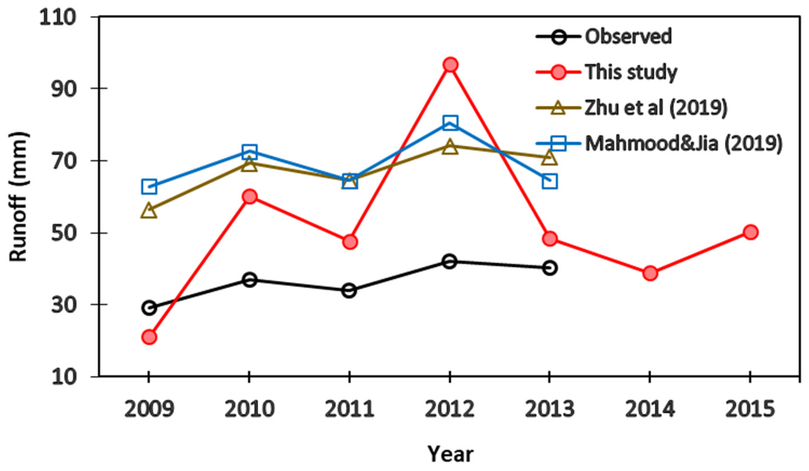
| Study | Time Period | Study Area | Mean Runoff (mm/Year) | |
|---|---|---|---|---|
| 1 | LCBC [75] | 1954–1969 | Lake Chad | 170.7 |
| 2 | Odada et al. [2] | Pre-1970 | Lake Chad | 90.8 |
| 3 | Vuillaume [79] | 1954–1969 | Chari-Logone Basin | 67.67 |
| 4 | Olivry et al. [77] | 1932–1995 | Chari-Logone Basin | 52.64 |
| 5 | Odada et al. [2] | 1971–1990 | Lake Chad | 42.22 |
| 6 | LCBC [75] | 1988–2010 | Lake Chad | 65.7 |
| 7 | Zhu et al. [25] | 1991–2013 | Southern Pool of Lake Chad | 40.52 |
| 8 | Mahamat Nour et al. [30] | 1960–2015 | Chari-Logone Basin | 42 |
| 9 | Lemoalle et al. [76] | 1960–2009 | Chari-Logone Basin | 41.35 |
| 10 | This study | 2009–2015 | Southern Lake Chad Basin | 51.9 |
Publisher’s Note: MDPI stays neutral with regard to jurisdictional claims in published maps and institutional affiliations. |
© 2022 by the authors. Licensee MDPI, Basel, Switzerland. This article is an open access article distributed under the terms and conditions of the Creative Commons Attribution (CC BY) license (https://creativecommons.org/licenses/by/4.0/).
Share and Cite
Bennour, A.; Jia, L.; Menenti, M.; Zheng, C.; Zeng, Y.; Asenso Barnieh, B.; Jiang, M. Calibration and Validation of SWAT Model by Using Hydrological Remote Sensing Observables in the Lake Chad Basin. Remote Sens. 2022, 14, 1511. https://0-doi-org.brum.beds.ac.uk/10.3390/rs14061511
Bennour A, Jia L, Menenti M, Zheng C, Zeng Y, Asenso Barnieh B, Jiang M. Calibration and Validation of SWAT Model by Using Hydrological Remote Sensing Observables in the Lake Chad Basin. Remote Sensing. 2022; 14(6):1511. https://0-doi-org.brum.beds.ac.uk/10.3390/rs14061511
Chicago/Turabian StyleBennour, Ali, Li Jia, Massimo Menenti, Chaolei Zheng, Yelong Zeng, Beatrice Asenso Barnieh, and Min Jiang. 2022. "Calibration and Validation of SWAT Model by Using Hydrological Remote Sensing Observables in the Lake Chad Basin" Remote Sensing 14, no. 6: 1511. https://0-doi-org.brum.beds.ac.uk/10.3390/rs14061511