1. Introduction
With the emergence of the new generation of aviation weapons, such as the fourth-generation fighters and unmanned combat aircraft, modern warfare will involve targets with stronger mobility, increasingly sophisticated escape methods, and low detection capabilities [
1]. To achieve accurate guidance and attack solutions for this type of strong maneuvering target, it is essential to estimate its state quickly and accurately. Meanwhile, modern radar sensors have shown the characteristics of high resolution and high detection accuracy, multiple measurements can be captured on the target surface at each sampling moment, thus the shape cannot be ignored anymore [
2]. That is to say, the state that needs to be estimated includes not only its kinematic state but also its extension state. In this paper, a new model set design method for the variable structure multiple-model estimation has been proposed to improve the tracking performance of the maneuvering extended target in air combats.
Any target tracking algorithm is built on the basis of a dynamic model. Selecting the appropriate dynamic models is an important entry point for target tracking, which can effectively improve its estimation performance [
3]. The development of a dynamic model is a process from simple to complex. In order to accommodate the complex maneuverability of the target, scholars have proposed models, such as the constant velocity (CV) model [
4], the constant acceleration (CA) model [
4], the constant turn (CT) model [
5], the semi-Markov model [
6], and the “current” statistics (CS) model [
7]. However, in the field of modern target tracking, a single mathematical model cannot be used for describing the kinematic state due to its complexity and variability.
Blom and Bar-Shalom first proposed the interactive multiple-model (IMM) algorithm [
8]. IMM is a fixed structure multiple-model (FSMM) algorithm. At any time, it uses several fixed models to perform parallel filtering, and the state estimation result is the weighted value of each output. Clearly, it is difficult to make use of the real-time information of the system. Only when the model set matches the true mode of the current system, it can be considered as the optimal estimation. Once the true system mode deviates from the current model structure, it might cause tracking failure. In order to obtain high accuracy, a large number of fixed models are often required to implement coverage of the true system mode. However, this inevitably will increase the amount of computation and lead to competition between models, thus resulting in decreased tracking accuracy [
9].
In order to overcome this dilemma, Professor Li and colleagues proposed the variable structure multiple-model (VSMM) algorithm in the 1990s for the first time [
10]. Compared to the pre-existing FSMM algorithm, the VSMM algorithm inherits the estimation and fusion steps of the multiple-model (MM) algorithm but involves an additional step of model set design. That is to say, its recursive process involves two tasks: model set adaptation (MSA) and MM sequence condition estimation, respectively. Among them, the purpose of MSA is to realize the dual self-adaptation of the model structure and the model number. The latter is responsible for estimating the target state by using multi-model estimation methods under the conditions of a given model set. It is obvious that the performance of the MM estimation algorithm depends largely on the model set used. Therefore, the research on model set design methods is of great significance.
The existing model set design methods are mainly divided into two aspects: (i) to design an over-complete model set and subsequently perform adaptive switching and selection among the model sets [
11], and (ii) to generate a new model set online in real-time based on the target state estimation [
12,
13,
14].
The adaptive strategies of the model group switching (MGS) algorithm and the likely-model set (LMS) algorithm adopt the first design idea. MGS adopts a model activation and termination approach, but its tracking performance is affected by the division and topology of the model set. Once the target maneuvers too fast, its performance will become poor. LMS can certainly reduce some computation while retaining the estimation accuracy, but it cannot activate models outside the total model set. Therefore, when the target maneuvers, there will be a high peak error. The expected-mode augmentation (EMA) algorithm is a model activation method, which adopts the second design idea. It activates an expected model, which is a probability-weighted sum of the basic models. The tracking performance of EMA is obviously better than that of the IMM algorithm, but it is only suitable for the model set with parameter change and cannot be directly used in the model set with structural change. The adaptive grid (AG) algorithm is a model self-learning algorithm in essence. It does not need to set the corresponding models in advance. The parameters of each model at
are weighted to generate new model parameters at
k to realize the time variation of the model set. Such algorithms and designs have mainly been included in a few previous studies [
15,
16,
17].
Lan et al. [
18] first proposed the best model augmentation (BMA) algorithm, and its adaptive strategy was realized based on Kullback–Leibler (KL) information [
19]. In this algorithm, the set of basic models, as well as candidate models, have been assumed to be known. The algorithm activates a “best” model from the candidate model set and adds it to the basic model set. The “best” here refers to the minimum difference between the model and the true system mode, which is measured by KL divergence. The smaller the value of KL, the smaller is the difference. BMA overcomes the defects of EMA and is widely used in situations with different model structures and parameters. However, there are still several problems that can be improved: (i) The KL criterion need to be frequently calculated each time the best model is activated from the candidate model set, resulting in a large computational burden. (ii) The models in the basic model set and the candidate model set are fixed, which means that the model parameters cannot be adjusted in real time according to the maneuvering state. (iii) The prior known information of the model set is introduced, that is, all dynamic models are known, thus the correction capability of the best model to the basic model set is limited.
To deal with the problem, this paper proposes a new model set design method by modifying the BMA algorithm. The main idea of the proposed method is as follows: Firstly, the basic model set is represented by a coarse grid without any prior setting, and the corresponding adaptive mechanism is applied to realize the time variation of the basic model set. Secondly, a uniformly quantized mode space is generated, centered on the best model at the above moment, and this is taken as the candidate model set at this moment. Due to the time-varying model set, the uncertainty caused by the assumption of prior knowledge in the traditional method can be effectively avoided, and the correction ability of the best model to the basic model set can also be further improved. Finally, the complex KL criterion in the traditional BMA algorithm is discarded, and a simpler mechanism based on similarity distance is adopted to select the best model. In the simulation experiment part, the single maneuvering extended target has been taken as the tracking target, and a digital simulation has been carried out in two scenarios. The simulation results show that this method can effectively avoid tracking failure and improve the estimation accuracy under strong maneuvering conditions.
The remainder of this paper is organized as follows. In the next section, we mainly complete the problem formulation and propose the modified BMA algorithm for VSMM based on adaptive grid.
Section 3 does the numerical simulation about the proposed method, wherein its tracking performances are illustrated in comparison to some existing approaches.
Section 4 discusses the experimental results.
Section 5 concludes the paper.
2. VSMM Algorithm Based on AG-BMA
2.1. Problem Formulation
The task of maneuvering extended target tracking involves estimating the target state based on the constructed mathematical model and the measured value obtained by the sensor. In this paper, the establishment of the mathematical model and the generation of the measurement points have been carried out in the two-dimensional Cartesian coordinate system. In addition, this paper mainly focuses on designing the model set for extended target tracking and proposes a modified best model augmentation algorithm based on adaptive grid (AG-BMA), in which the clutter and missed detection problems are not involved.
Assuming that the state vector, , of the target includes the motion variable, , and the shape variable, . The kinematic state of the target is represented by a random variable , where and represent the position and velocity of the target centroid, respectively.
For a linear jump Markov system, the transfer process between states can be formulated as follows:
where
and
represent the state transition matrix of the motion variable and the morphological variable,
and
represent the covariance matrices of the process noise,
and
are the independent process noise.
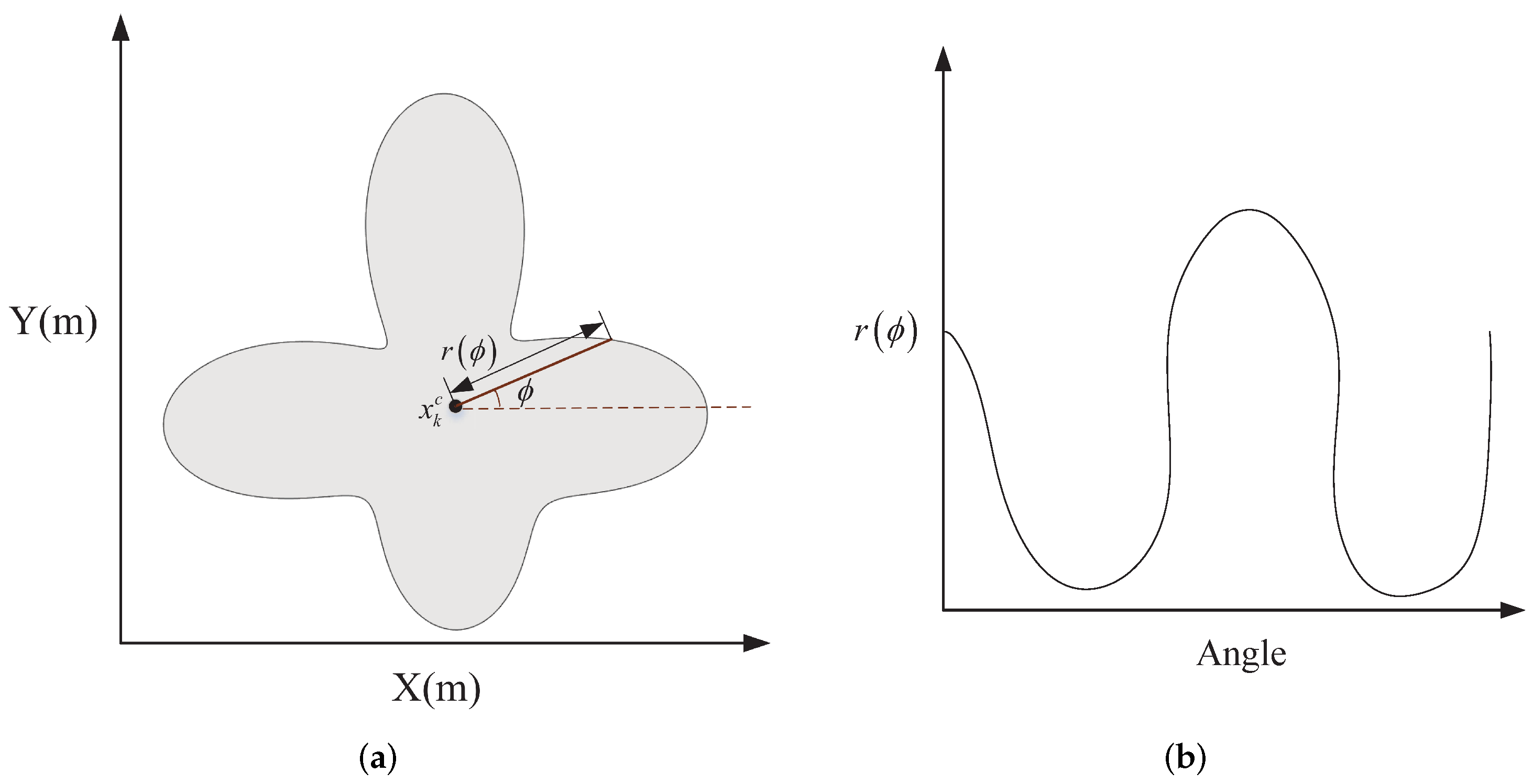
2.1.1. Star-Convex Extended Target
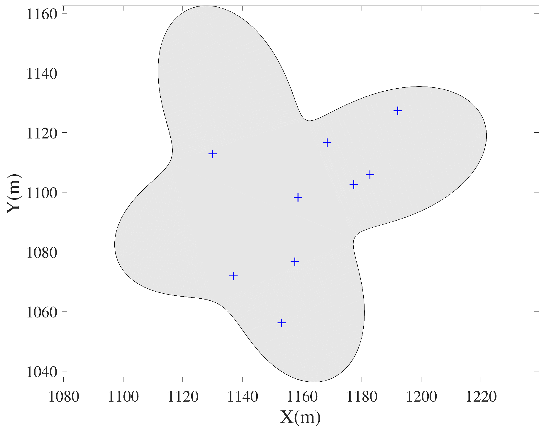
In many real applications, there is a pressing need for incorporating the target shape information into target tracking to improve performance. In addition, knowledge of the target shape is also beneficial for target classification and identification. For extended target tracking, many approaches mainly differ in target shape models for the unknown true shape. However, they usually consider using some basic shapes, such as ellipse, rectangle, and so on. In recent years, there is a novel extended target model which describes the target approximately using star-convex shape [
20]. It has an advantage over the other shape modeling methods, because more detailed shape information can be described and utilized, e.g., the real shape of the aircraft can be approximated by the star-convex more accurately than other shapes.
In this paper, the random hypersurface model (RHM) has been used to represent the shape parameters of a star-convex extended target [
21]. By changing these parameters, the shape can be fitted arbitrarily [
22]. The contour,
, of the star-convex extended target can be described by a radial function,
, the size of which represents the distance between each contour point and the centroid
[
23]. The details of the model are shown in
Figure 1.
Then, the target contour can be described as follows:
where the scaling factor,
, is uniformly distributed in the interval
,
represents the angle formed by the ray from the centroid,
, to the contour point and the X-axis,
.
The radial function is expanded as a Fourier series, resulting in the following expressions:
Therefore, the shape parameters of the target can be obtained after parameterization by the relevant Fourier coefficients.
2.1.2. Measurement Model
The measurement sources drawn from the surface of the extended target are uniformly distributed. Additionally, it is the location of the measurement source with noise. In this paper, the measurement source has been modeled with RHM. It has been assumed that each scan will result in random
independent position measurements, which can be defined as follows:
where
is the observation matrix,
represents the position of measurement points, and
is the independent measurement noise. Both
and
belong to the unrelated zero-mean Gaussian white noise sequences.
2.1.3. Model Jump Sequences
The jump between models follows the first-order Markov process, and the Markov chain is homogeneous. Assuming that the model matching mode,
, at
is
and the model matching mode,
, at
k is
, then the transition probability from the model
to the model
is denoted as
.
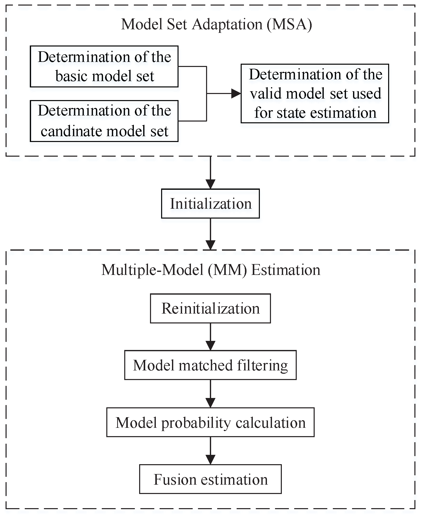
The implementation steps of the VSMM algorithm, based on AG-BMA, proposed in this work are shown in
Figure 2. In this chapter, the tasks to be completed can be divided into the following two parts:
- (1)
MSA . where is the basic model set, is the activated best model, and represents the valid model set used for MM estimation;
- (2)
MM estimation . It is responsible for a recursive calculation of the model set and at and k, respectively.
Figure 2.
Framework of the VSMM algorithm based on AG-BMA.
Figure 2.
Framework of the VSMM algorithm based on AG-BMA.
The former is responsible for determining a set of models for MM estimation, whereas the latter is responsible for estimating the target state under the conditions of a given model set. Next, the detailed process of MSA and MM estimation will be given in
Section 2.2 and
Section 2.3, respectively.
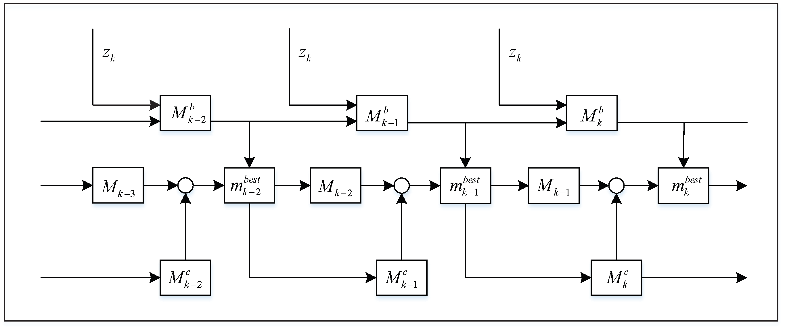
2.2. MSA
When the AG-BMA method is used for the model set design, its recursive flow can be described, as shown in
Figure 3. where
,
, and
are the basic model set at
,
, and
k, respectively.
,
, and
represent the candidate model set at
,
, and
k, respectively.
,
, and
denote the best model activated from
,
, and
, respectively.
,
, and
represent the valid model set.
In this section, the adaptive methods of basic model set, candidate model set, and valid model set are introduced in detail, respectively. Given space constraints, the following only takes the CA model framework as an example to introduce the corresponding steps.
2.2.1. Basic MSA
- (1)
Initialize a rough grid.
Assuming that the acceleration (m/s
) is
, and it ranges from
to
. In order to cover the mode space to the maximum extent, the maximum values of acceleration are taken as the initial value of the grid. In addition, the model interval is set as
, the threshold parameter of the impossible model is
, and
is the threshold parameter of the model jump. In other words, if the model probability is less than
, it is considered that the model does not match the current maneuvering state. If the model probability is greater than
, it can be considered that the model has a high degree of matching with the current maneuvering state.
where
is the initial center model,
,
,
, and
represent the initial left, right, upper, and lower edge models, respectively.
- (2)
The adaptive rules.
From to k, the following will introduce the adaptive rules for the grid.
Part 1: Adaptation of the grid center. Suppose that the model set parameters at
are
and their corresponding model probabilities are
,
,
,
and
, respectively. Then, the central value parameters of the grid are
Part 2: Adaptation of the grid edge. If,
, it indicates that the central model is closest to the true system mode. At this point, if
,
,
, and
are all smaller than
, it indicates that the left, right, upper, and lower edge models deviate from the current state of the system. Then, the model interval is reduced to
. Otherwise, the model interval remains unchanged. The jump rule is formulated as follows:
If
, it indicates that the left edge model is closest to the true system mode, all the other three edge models keep the original model interval. At this time, if
is greater than
, it can be considered that the difference between the left edge model and the system true mode is the smallest. In other words, the velocity in the X direction is constantly decreasing and the left edge model jumps
to the left. Otherwise, let the left edge model jump
to the left. The jump rule is formulated as follows:
If
, it indicates that the right edge model is closest to the true system mode, the other three edge models keep the original model interval. At this point, the jump rule of the right edge model is similar to that of the left edge model, which can be formulated as follows:
If
, it indicates that the upper edge model is closest to the true system mode, the other three edge models keep the original model interval. At this time, if
is greater than
, it can be considered that the upper edge model has the highest matching degree with the true system mode. In other words, the velocity in the Y direction is constantly increasing, and the upper edge model jumps up
. Otherwise, let the upper edge model jump up
. The jump rule can be formulated as follows:
If
, it indicates that the lower edge model is closest to the true system mode. Its adaptive rules are similar to those of the upper edge model, which can be formulated as follows:
where
,
,
,
,
refers to the minimum distance between each model, which not only ensures the comprehensiveness of the mode space but also maintains the independence between models.
The above describes how to use the grid to realize the adaptation of the basic model set, and the inspiration of its adaptive strategy mainly comes from literature [
24]. Based on the adaptive mechanism, a basic model set
that adapt well to the maneuvering state can be generated in real-time. On the one hand, the distribution of these models is relatively concentrated. On the other hand, the number of models is relatively small.
2.2.2. Candidate MSA
The determination of the candidate model set can also utilize the AG technology, where the parameters of each model slide adaptively over a continuous region. Therefore, only a small number of models related to the system mode are required at any one time.
In this paper, five CA models are selected to form the candidate model set, and each model corresponds to different maneuvering levels. Assuming that the best model activated at
is
, and the candidate model set at time
k is
, then horizontal, as well as vertical adaptation are required. The candidate model set at
k is
where
is the distance between the models in the candidate model set,
. In this way, the candidate model set can be fine-tuned and closer to the true system mode, resulting in the powerful modification of the best model to the basic model set.
2.2.3. Valid MSA
The valid model set used for MM estimation at
k can be obtained by
. where, the best model,
, is activated from the candidate model set,
. Additionally, the “best” here refers to the minimum difference between the model and the true system mode. In this paper, the complex KL criterion in the traditional BMA algorithm is discarded, and a simpler mechanism based on similarity distance is adopted to quantify this difference. The smaller the value of the Euclidean distance, the smaller is the difference [
25]. The process can be formulated as follows:
Among them, since the true mode,
, of the system is often unavailable, it can only be approximated with some prior information. In this paper, the expected model has been used to approximate the true system mode [
24]. Based on the idea of finding the expected model in the EMA algorithm, it can be thought of as a weighted sum of probabilities,
.
where
is the probability of the model
, and
is the valid model set at
.
In all, the complete pseudo codes for the above MSA algorithm can be summarized in Algorithm 1.
| Algorithm 1: Pseudo codes for the proposed MSA algorithm. |
| ➀ Basic model set adaption |
| , where represents the initial model set. |
| Part 1: Adaptation of the grid center. |
| Suppose that the model set parameters at are and their |
| corresponding model probabilities are , , , and , respectively. Then, |
| . |
| Part 2: Adaptation of the grid edge. |
| When , then execute Equation (11); |
| When , then execute Equation (12); |
| When , then execute Equation (13); |
| When , then execute Equation (14); |
| When , then execute Equation (15). |
| ➁ Candidate model set adaption |
| The candidate mode set can be formulated as Equation (16), where represents |
| the best model at the above moment. |
| ➂ Determination of the valid model set |
| The approximate true system mode is ; |
| The activated best model can be obtained by ; |
| The valid model set is . |
| Then, , return to step ➀ and proceed to the next iteration. |
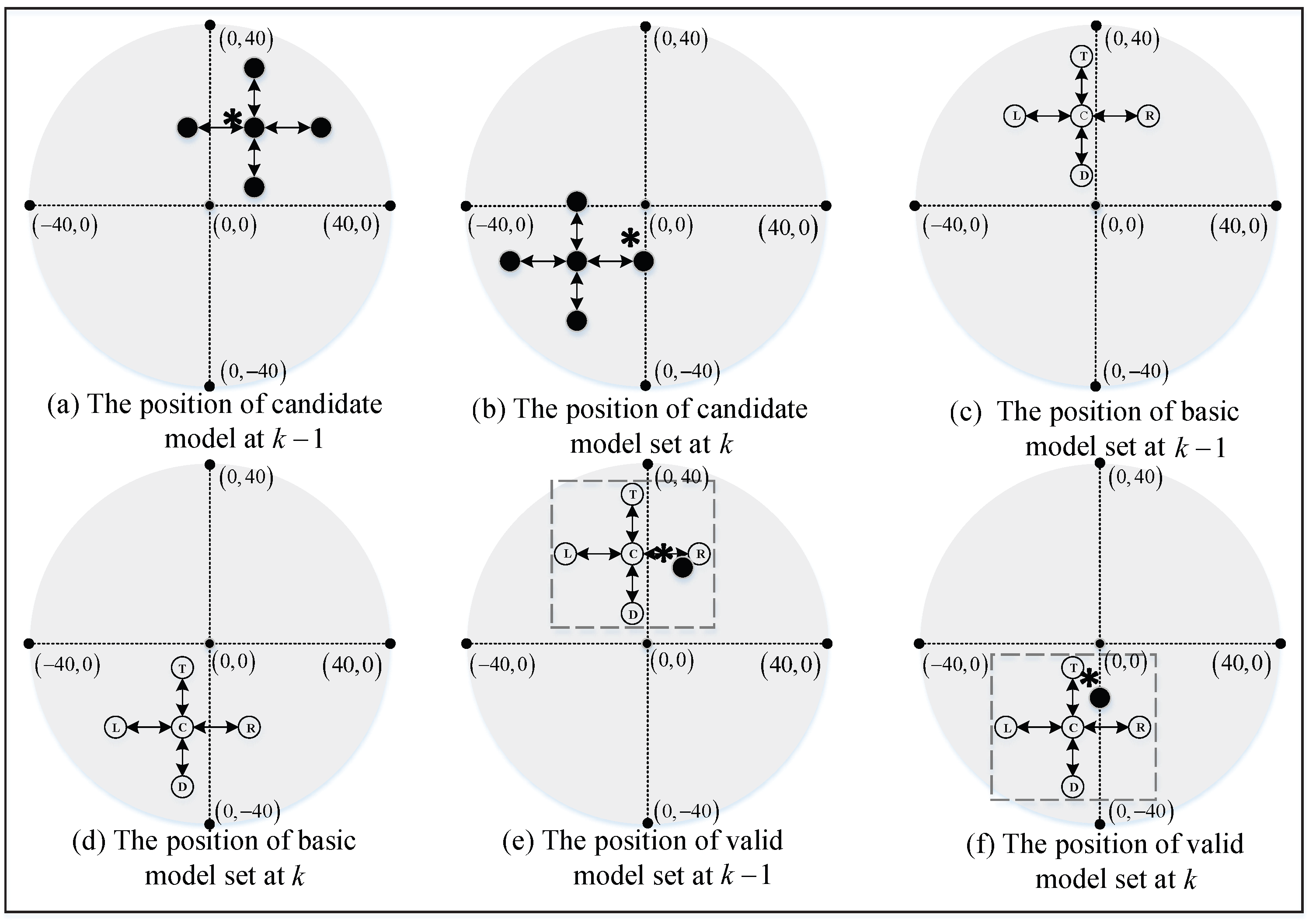
To visualize the whole model set design process, the topology of the AG-BMA algorithm is shown in
Figure 4. In the simulated well-known examples of [
12,
26,
27], the maximum acceleration in any coordinate direction is assumed to be 4 g (g = 10 m/s
). Thus, the mode space can be defined as follows:
Moreover, a more intuitive explanation of the position is given. Here, we use the circular areas (the center of the circle is
and the radius is 40 (m)) to represent the entire mode space
. The coordinates
of any point in the region can represent a kind of motion mode, where
and
represent the acceleration (m/s
) of the target in the X-axis and Y-axis direction, respectively. For example, the coordinate point
indicates a motion that the constant deceleration with an acceleration of 40 (m/s
) in the X-axis direction and the constant velocity in the Y-axis direction.
Figure 4a,b represent the positions of the candidate model sets at
and
k in the entire mode space, in which the symbol ‘∗’ denotes the true system mode and these black circles form the candidate model set.
Figure 4c,d represent the positions of the basic model set at
and
k, where these white circles represent four edge models and one center model, respectively.
Figure 4e,f represent the valid model set, in which the black circle denotes the best model augmented from the candidate model set. The models in the valid model set will be used to perform the MM estimation in
Section 2.3. It is not difficult to see that the candidate model set and the basic model set have formed a double-layer coverage near the true system mode. The valid model set at the current moment is only composed of the best model and the basic model set, thus the true mode ‘∗’ of the system can be maximally approximated with fewer models.
2.3. MM Estimation
Based on the valid model set at
k, MM
is run to obtain the filtering results,
,
, of each model and calculate the model probability,
. The multi-model estimator uses the simplest reinitialization method. First of all, the last state estimation,
, and its covariance matrix,
, are taken as the common initial inputs. Then, each model performs its own state estimation using the basic filtering algorithm and calculates the probability of each model. Finally, the state estimation result and its error covariance matrix are obtained by weighted summation. Its algorithm structure is shown in
Figure 5.
For , the loop is as follows:
2.3.1. Reinitialization of the Model Conditions
Since each model filter can be a valid system model filter, the initial conditions of each filter are based on the synthesis of the filtering results of the previous model. Then, the input of the
model filter after reinitialization [
28] is
Assuming that the matching model at
is
and the matching model at
k is
, Equation (
22) represents the mixed probability under the condition of
. Where
,
is the matching probability of the model
i and the true system mode at
.
2.3.2. Model Conditional Filtering
Given the initial state and the covariance matrix, the next step is to update the state estimation according to the new measurements
obtained at
k. Assume that the model
is adopted at
and the model
is adopted at the moment
k. Further, taking
from Equation (
20) and
from Equation (
21) as the initial values, the state estimation,
, and its covariance matrix,
, are calculated by using the models matching with the true system mode and their corresponding filtering equation.
(1) State prediction:
For
, calculate separately
(2) Measurement prediction residual, , and its covariance calculation:
The likelihood function matching
is calculated as follows:
Under the Gauss hypothesis, the likelihood function can be calculated as follows:
(3) Update of the filtering results:
For
, the filter gain array, the updated status estimation result, and its error covariance are calculated as follows:
where
is the Kalman gain.
(4) Update of the model probabilities:
For
, the model probability is calculated as follows:
where
,
,
represents the likelihood function matching model
.
(5) Estimation of fusion:
While synthesizing the estimation results of each model, the updated model probability is used as the weight coefficient. Then, the overall estimation and its error covariance matrix at is formulated as follows:
where
is the updated state estimation result of the
filter.
As for the moment at k, the VSMM algorithm based on AG-BMA method completes an iteration process. Additionally, then, , return to step (1) and proceed to the next iteration.
3. Simulation Results
In order to prove that the proposed method is effective in improving the estimation performance of the kinematic state and the extension state, an extended target with star-convex shape, as shown in
Figure 6, was used in this paper. Assuming that the measurement sources are all distributed on the target surface, and the radar sensor with high resolution capability and detection accuracy obtains the information. The tracking object of this paper is a single maneuvering extended target, which does not involve clutter and missed detection.
The performance of the proposed VSMM algorithm based on AG-BMA was investigated over a deterministic maneuver scenario and a random scenario. The two scenarios enable the evaluation of the kinematic state and the shape estimation performance of the algorithm, which can be judged based on the root-mean-square error and Hausdorff distance, respectively. In addition, the proposed algorithm has been compared with the IMM algorithm and two other VSMM algorithms to illustrate its effectiveness.
Here, we need to emphasize the formula of Hausdorff distance
between the estimated shape
and the real shape
, where
C and
represent the estimated target and the real target, respectively. The radial function that used to describe star-convex is characterized by its extension parameter vector
, i.e.,
where
is a continuous set and can be replaced by a discrete set with the idea of angular uniform discretization.
where
is the number of samples. Accordingly,
and
can be expressed as
Then, the formula of Hausdorff distance is [
29]
where
a and
represent a point of the estimated shape and the real shape, respectively.
denotes the Euclidean distance between point
a and each point in
,
denotes the Euclidean distance between point
and each point in
.
3.1. Deterministic Scenario
In order to demonstrate the general applicability and universality of the proposed algorithm, a deterministic scenario (DS) was introduced. The simulation was carried out under the framework of the CT and CV models, in which the structure and parameters were all changed.
Table 1 lists the kinematic state of the target, namely the serpentine turning process. The parameter settings of the CT models with different turning rates were as follows:
When using the proposed AG-BMA-based VSMM algorithm for state estimation, the adaptive process of the model set was different from that of the CA model framework introduced in
Section 2.2. Suppose that the turning rate of the target is
w and its range of variation is
, then the boundary values of the turning rate are taken as the initial value of the grid, and only horizontal self-adaptation is required.
When the basic model set was used, the number of models was set to 3. The model set at the initial time was set to , where . The adaptive steps of the grid center and the grid distance were similar to those of the constant acceleration scenarios, and, thus, a detailed description has not been given here. Eventually, an adaptive model set, , was obtained, which was generated in real-time according to the maneuvering state of the target.
Similarly, three CT models were selected to form the candidate model set, and the turning rate of each model corresponded to different maneuvering levels. If the best model activated at is , then the set of candidate models at k can be defined as . In this paper, was taken to be 5 rad/s in order to achieve fine tuning.
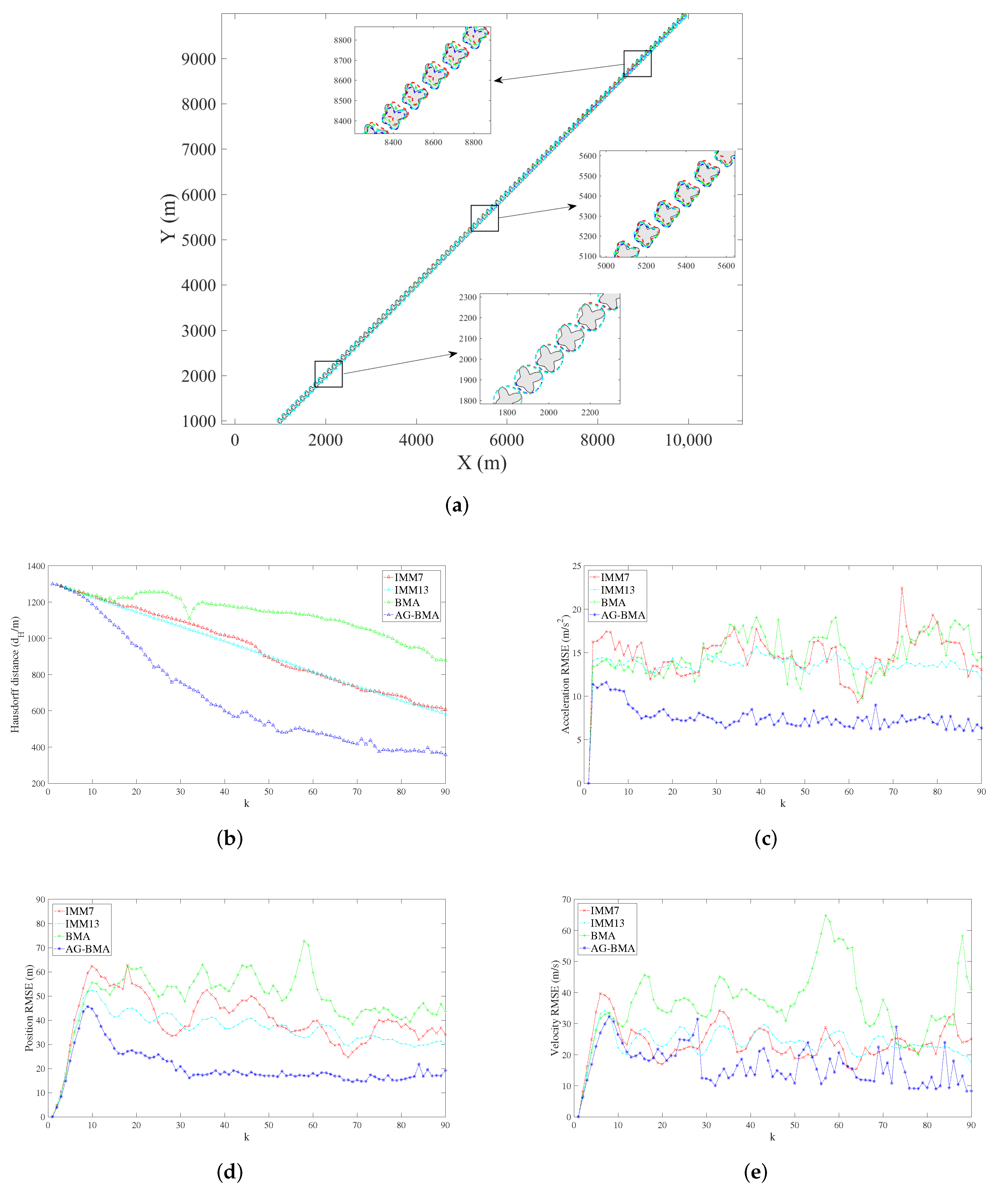
Figure 7 depicts the comparative results between the three algorithms, namely, IMM, BMA, and AG-BMA, over 100 Monte Carlo runs. Hausdorff distance and root-mean-square error are used to evaluate the performance of the algorithm. The smaller their values, the better is the tracking performance of the corresponding algorithm.
The root-mean-square error values (unit: m, m/s) and the computational load of the three algorithms are given in
Table 2 and
Table 3, respectively.
Figure 7a,b show the estimation performance of the extension state. From the results, it can be inferred that BMA provides the poor shape estimation performance. Furthermore, the tracking performance of the three algorithms is largely consistent in the non-maneuvering stage. However, in the maneuvering stage, the AG-BMA algorithm exhibits superior performance in shape estimation. As shown in
Figure 7a, the shape estimated by the AG-BMA algorithm is closer to the true shape of the target.
Figure 7c,d show the root-mean-square error comparison of the centroid position and velocity resulting from the application of the three algorithms. From the results, it can be seen that the proposed AG-BMA algorithm can better improve the estimation performance of the kinematic state. This is mainly because the AG-BMA algorithm can automatically adjust the parameters of each model in the basic and candidate model set depending on the maneuvering condition in order to efficiently match the true system mode. However, the results show that even without activating a new model, the IMM algorithm still has a smaller estimation error than BMA sometimes. The reasons for this result can be summarized as follows: On the one hand, the BMA algorithm can achieve optimal estimation only when the true system mode is in the whole mode space. On the other hand, this could be because the model contained in the IMM algorithm happens to be able to describe part of the true system mode.
3.2. Random Scenario
To provide a performance comparison over an ensemble of maneuver trajectories that is as fair as possible, the algorithms were tested on the random scenario (RS) that has been developed in previous studies [
26,
30]. In the entire simulation process, the target performed random acceleration motion, and thus it can be regarded as a continuous strong maneuvering process. Here, the acceleration vector is a two-dimensional semi-Markov process and it jumps from one state of acceleration of magnitude
and phase
to another after a random time interval. Obviously, such strong maneuvering scenarios put higher demands on the performance of the MM estimators.
The specific model assumptions in this scenario were as follows: The program executed 90 simulation steps each time and the acceleration changed 10 times in the entire process. Then, the residence time,
, of the state
was a random number up to 90 and satisfied the condition
. The phase angle,
, obeyed a Gaussian distribution with mean,
, and variance,
. In this simulation scenario, the parameters were set as follows:
Figure 8 depicts the comparative results of the four algorithms, IMM7, IMM13, BMA, and AG-BMA, over 100 Monte Carlo runs for an random scenario. The Hausdorff distance and the root-mean-square error were used as the evaluation metrics for accessing the estimation results of the extension state and kinematic state, respectively. The smaller their values, the better is the tracking performance of the corresponding algorithm.
The root-mean-square error and the computational load corresponding to the four algorithms are given in
Table 4 and
Table 5, respectively.
Figure 8a,b show the performance of four algorithms for shape estimation. The smaller the Hausdorff distance is, the better the shape estimation is. Obviously, the extension state estimated by AG-BMA algorithm is closer to the true shape of the target.
From the results presented in
Table 4 and
Table 5, it can be seen that the original BMA algorithm exhibits the poor estimation accuracy and also has a large computational burden. The reasons for this result can be summed up as follows: On one hand, the KL information needs to be frequently calculated each time the best model is activated. On the other hand, it is due to the uncertainty caused by its fixed and prior known model set. Although the IMM7 algorithm requires the shortest computational time, its estimation error is bigger than IMM13 and AG-BMA. IMM13 can cover the entire model space to a large extent due to a large number of models, but it is still less effective than AG-BMA, and it also requires the largest amount of calculation. Undoubtedly, the key to improving the tracking accuracy is to ensure that the dynamic model used is as close as possible to the true system mode of the target. Fortunately, the proposed AG-BMA algorithm can construct an adaptive model set online based on the information of the previous moment. Thus, the AG-BMA algorithm can obtain the best estimation performance of kinematic state among the four algorithms.
5. Conclusions
To improve the tracking accuracy of the maneuvering extended target, a new model set design method, namely, AG-BMA, has been proposed in this work. This method utilizes an adaptive grid to achieve a dual adaptation of the basic and candidate model sets so that it can approximate the true system mode to a large extent with a small number of models. Furthermore, it can effectively overcome the model mismatch caused by strong maneuvering. In this paper, the proposed algorithm was simulated in a deterministic scenario and a random scenario to prove the effectiveness of the method. From the simulation results, it can be concluded that the proposed AG-BMA algorithm can effectively improve the estimation accuracy of the extended shape and centroid motion.
How to designing an effective model set for multiple maneuvering extended targets tracking is still challenging. The proposed model set designing method (i.e., AG-BMA) has room for further development and improvement. As our research directions to next step, we will consider modifying AG-BMA and apply it to tracking of multiple maneuvering extended targets. In this context, more work remains to be completed.


