Multi-Target Localization of MIMO Radar with Widely Separated Antennas on Moving Platforms Based on Expectation Maximization Algorithm

Abstract

This paper focuses on multi-target parameter estimation of multiple-input multiple-output (MIMO) radar with widely separated antennas on moving platforms. Aiming at the superimposed signals caused by multi-targets, the well-known expectation maximization (EM) is used in this paper. Target’s radar cross-section (RCS) spatial variations, different path losses and spatially-non-white noise appear because of the widely separated antennas. These variables are collectively referred to as signal-to-noise ratio (SNR) fluctuations. To estimate the echo delay/Doppler shift and SNR, the Q function of EM algorithm is extended. In addition, to reduce the computational complexity of EM algorithm, the gradient descent is used in M-step of EM algorithm. The modified EM algorithm is called generalized adaptive EM (GAEM) algorithm. Then, a weighted iterative least squares (WILS) algorithm is used to jointly estimate the target positions and velocities based on the results of GAEM algorithm. This paper also derives the Cramér-Rao bound (CRB) in such a non-ideal environment. Finally, extensive numerical simulations are carried out to validate the effectiveness of the proposed algorithm.

1. Introduction

Recent years have witnessed a rapid development in signal processing technologies for array or multi-node radar systems, such as space-time adaptive processing radar [1,2], distributed coherent radar [3], multiple-input multiple-output (MIMO) radar with co-located antennas [4] and MIMO radar with widely separated antennas [5,6,7,8,9]. Among them, MIMO radar with widely separated antennas simultaneously observes the target from multiple different angles, thus reducing the probability that all antennas measure small radar cross-section (RCS) and low Doppler shift [10]. Furthermore, putting these antennas on moving platforms can ensure the radar system gets superior sensing opportunities. For example, in an urban area where targets may be obscured by buildings, the moving radars can arrive in more suitable positions to obtain the target information [11]. Hence, this paper concerns multi-target localization of MIMO radar with widely separated antennas on moving platforms.

In the field of target localization based on MIMO radar with widely separated antennas, Ref. [7] analyzes the possibility of high-precision target localization through the derivation of Cramér-Rao bound (CRB) and ambiguity function. Ref. [10] studies the optimized system/configuration design based on CRB. Ref. [12] uses the best linear unbiased estimator to analyze the geometric dilution of precision (GDOP) of target location for MIMO radar with widely separated antennas. Ref. [13] analyzes the effect of phase error on target positioning accuracy through CRB. For the CRB derivation and parameter estimation of these articles, the key assumptions are that the target echoes are orthogonal and the echo signal-to-noise ratios (SNRs) in different propagation paths are the same, or the SNRs are known. These assumptions bring simplicity to theoretical derivation and algorithm implementation. However, in some scenarios, these assumptions are unrealistic. First of all, in a multi-target scenario, if the observed target continues to move, it is very likely that the two targets are close to each other [14], resulting in superimposed signals. Secondly, because each receiver cannot be exactly the same, each receiver has a different noise variance, which is named as spatially-non-white noise. At the same time, due to the large distance between radar nodes, the propagation paths (transmitter to target to receiver) are different for different radar nodes or targets, which means the path losses are different. In addition, some targets have a rich scattering environment yielding 5∼20 dB target RCS fluctuations [6], namely, target’s RCS spatial variations, which is easily observed in widely separated antennas. Thus, the SNRs in the different propagation paths are different.

Aiming at superimposed signals, expectation maximization (EM) algorithm is applied in [15]. The idea of EM algorithm is to decompose the observed data into its signal components (E-step) and then estimate the parameters of each signal component separately (M-step). E-step in EM algorithm is model-oriented. To estimate the target position parameter and SNR, the E-step should be derived to obtain a Q function based on the signal model. Refs. [16,17,18] improve the Q function of EM algorithm. However, Refs. [16,17,18] are based on the model of half-wavelength array, which are not applied to MIMO radar with widely separated antennas. M-step in EM algorithm is the solution of estimator, which is algorithm-oriented. Refs. [15,19] implement the M-step based on the grid point search method. The precision of the grid point search method is determined by the grid interval. To ensure good estimation accuracy, dense grid partitioning is required, which brings high computational complexity. Refs. [20,21,22,23] combine the Newton iterative algorithm and M-step, and expand the data information matrix in the iteration to a complete data information matrix. However, Newton method is prohibitively expensive in high-dimensional problems as they involve the storage and handling of approximate Hessian matrix [24]. In summary, for MIMO radar with widely separated antennas, the Q function of E-step related to the echo delay/Doppler shift and SNR estimation needs to be derived. In addition, for the M-step, it is necessary to further minimize the computational complexity.

This paper refers to different SNRs in different propagation paths as the SNR fluctuations. SNR fluctuations mean that the reliability of target echo delay and Doppler shift estimation is different. For example, if the delay and Doppler shift are estimated from higher SNR echo signal, the estimated results are more reliable. Hence, for the estimation of the target or radar location based on the echo delays and Doppler shifts, the delay and Doppler parameters that have higher reliability need to be assigned a larger weight. Refs. [25,26,27,28,29] locate the target based on the estimated echo delay. Ref. [25] uses the least square algorithm to locate targets. Refs. [26,27] propose neural network to achieve target location. However, Refs. [25,26,27] do not consider the influence of SNR fluctuations on target localization. Refs. [28,29] propose a target localization algorithm considering the influence of radar receiver noise. However, they do not estimate the SNRs from received waveform because the SNRs are assumed to be known in these papers. Ref. [30] analyzes SNR fluctuations in MIMO radar with widely separated antennas, but Ref. [30] focuses on the field of target detection.

This paper focuses on practical problems of target localization in MIMO radars, such as dense multi-target and SNR fluctuations. Firstly, to estimate the echo delay/Doppler shift and SNR, the Q function of EM algorithm is derived. Secondly, the gradient descent is used in M-step to reduce the computational complexity. The modified EM algorithm proposed in this paper is called generalized adaptive EM (GAEM) algorithm. Then, a weighted iterative least squares (WILS) algorithm is used to estimate the target positions and velocities based on the results of the GAEM algorithm. In addition, the CRB in the non-ideal environment is derived. Finally, numerical simulations are conducted to verify the proposed algorithm.

The rest of the paper is organized as follows: Section 2 firstly establishes the signal model which exists the superimposed signal and SNR fluctuations. Then, the GAEM algorithm is proposed, and CRB is derived. Section 3 verifies the feasibility of the algorithm through numerical simulations. Section 4 and Section 5 draw the discussion and conclusion, respectively.

2. Materials and Methods

2.1. Signal Model

Figure 1 shows an application scenario of MIMO radar with widely separated antennas on moving platforms. The radar system contains multiple radar nodes on moving platforms, and the distance between radar nodes is much larger than half wavelength. As shown in Figure 1, multiple radar nodes are mounted on the unmanned aerial vehicle (UAV) and shuttle between buildings to approach the target, thereby completing the estimation of target parameters. However, due to the large distance between radar nodes, the propagation paths of the echoes received by different radar nodes are different. When the building blocks the echo signal of a certain propagation path, the echo SNR of this propagation path will be much lower than the echo SNR of other propagation path. As a result, the reliability of the target information carried by the echo in this propagation path decreases. At the same time, the targets (such as cars) in the urban scene are densely distributed. The generated superimposed signals have an impact on the target positioning.

Topology diagram of MIMO radar and targets is shown in Figure 2, which shows two practical problems concerned in this paper: (1) target echo overlap, (2) different SNR caused by different radar receiver noises and different propagation paths. Let K, L, and $Q_0$ denote the total number of transmitting radar nodes, receiving radar nodes, and targets, respectively. Further, ${\tau }_{lk}^q$ and $f_{lk}^q$ represent the delay and Doppler shift transmitted by the kth radar node, reflected by the qth target and received by the lth radar node, respectively. Suppose that the coordinates of the kth transmitter and lth receiver are ${\mathit{p}}_k^t={\left[x_k^t,y_k^t\right]}^T$ and ${\mathit{p}}_l^r={\left[x_l^r,y_l^r\right]}^T$, respectively, and the velocities of the kth transmitter and lth receiver are ${\mathit{v}}_k^t={\left[v_{x_k^t},v_{y_k^t}\right]}^T$ and ${\mathit{v}}_l^r={\left[v_{x_l^r},v_{y_l^r}\right]}^T$, respectively. we denote superscript T as the transpose.

Let ${\mathit{p}}_q={\left[r_0^{q}sin{\theta }_0^q,r_0^{q}cos{\theta }_0^q\right]}^T$ and ${\mathit{v}}_q=\left[v_r^{q}sin{\theta }_0^q+v_{\theta }^{q}cos{\theta }_0^q,\right.$ ${\left.v_r^{q}cos{\theta }_0^q-v_{\theta }^{q}sin{\theta }_0^q\right]}^T$ denote the location and velocity of the qth target, respectively. Then, the echo delay is related only to the distance between the radar node and the target, i.e.,

$${\tau }_{lk}^q=\frac{1}{c}\left({∥{\mathit{p}}_q-{\mathit{p}}_l^r∥}_2+{∥{\mathit{p}}_q-{\mathit{p}}_k^t∥}_2\right),$$

(1)

where c denotes the speed of light in free space; ${∥·∥}_2$ represents the $l_2$ norm.

The echo Doppler shift is related only to the projection of the velocity (radar velocity and target velocity) in the radar-target direction, i.e.,

$$f_{lk}^q=\frac{{\left({\mathit{v}}_q-{\mathit{v}}_l^r\right)}^T\left({\mathit{p}}_q-{\mathit{p}}_l^r\right)}{\lambda {∥{\mathit{p}}_q-{\mathit{p}}_l^r∥}_2}+\frac{{\left({\mathit{v}}_q-{\mathit{v}}_k^t\right)}^T\left({\mathit{p}}_q-{\mathit{p}}_k^t\right)}{\lambda {∥{\mathit{p}}_q-{\mathit{p}}_k^t∥}_2},$$

(2)

where $\lambda$ denotes the wavelength of the carrier frequency.

Let ${\left[{\tilde{x}}_l^r,{\tilde{y}}_l^r\right]}^T$, ${\left[\Delta x_l^r,\Delta y_l^r\right]}^T$, ${\left[{\tilde{v}}_{x_l^r},{\tilde{v}}_{y_l^r}\right]}^T$ and ${\left[\Delta v_{x_l^r},\Delta v_{y_l^r}\right]}^T$ be the nominal position, position deviation, nominal velocity, and velocity deviation of the lth receiving radar, respectively. Then, we define

$$\begin{array}{c}{x}_l^r={\tilde{x}}_l^r+\Delta x_l^r,y_l^r={\tilde{y}}_l^r+\Delta y_l^r,\\ v_{x_l^r}={\tilde{v}}_{x_l^r}+\Delta v_{x_l^r},v_{y_l^r}={\tilde{v}}_{y_l^r}+\Delta v_{y_l^r}.\end{array}$$

(3)

The system deviation definition of the kth transmitting radar node is similar to that in (3). Let the number of slow times be M. Let $f_s$ denote the sampling frequency of radar system. Then, the received waveform at the lth receiver, time $n/f_s$ and mth pulse is

$$y_{lm}\left[n\right]=\sqrt{\frac{E}{K}}\sum _{q=1}^{Q_0}\sum _{k=1}^K{\xi }_{lk}^q{s}_k\left[n;{\tau }_{lk}^q\right]e^{-j2\pi f_c{\tau }_{lk}^q-j2\pi m\mathrm{PRI}{f}_{lk}^q+j{\varphi }_{lk}^q}+w_{lm}\left[n\right],$$

(4)

where E is the total energy transmitted by MIMO radar; ${\xi }_{lk}^q$ represents the target reflection coefficient multiplied by path loss; $s_k\left[n\right]$ represents the waveform emitted by the kth transmitter; $\mathrm{PRI}$ is the pulse repetition interval; ${\varphi }_{lk}^q$ is the phase deviation; $w_{lm}\left[n\right]$ is the complex white Gaussian noise with zero mean and variance of ${\left({\sigma }_{wl}\right)}^2$. Suppose $s_k\left[n\right]$ is a unit energy waveform that satisfies ${\sum }_{n=0}^{N-1}{\left|s_k\left[n\right]\right|}^2/f_s=1$, where $N=\mathrm{PRI}·f_s$.

In order to simplify the solution process of the gradient descent algorithm, the echo signal can be transformed to the frequency domain. This means that the envelope movement among the radar nodes is converted to a phase shift in the frequency domain. The Fourier transform of (4) is

$$Y_{lm}\left[u\right]=\sqrt{\frac{E}{K}}\sum _{q=1}^{Q_0}\sum _{k=1}^K{\eta }_{lk}^q{S}_k\left[u\right]e^{-j2\pi u/N{f}_s{\tau }_{lk}^q-j2\pi m\mathrm{PRI}{f}_{lk}^q}+{\varsigma }_{lm}\left[u\right],$$

(5)

where $S_k\left[u\right]$ denotes the Fourier transform of $s_k\left[n\right]$; ${\eta }_{lk}^q$ denotes ${\xi }_{lk}^q{e}^{-j2\pi f_c{\tau }_{lk}^q+j{\varphi }_{lk}^q}$; ${\varsigma }_{lm}\left[u\right]$ is the Fourier transform of $w_{lm}\left[n\right]$. Because of the linear transformation properties of the Fourier transform, $w_{lm}\left[n\right]$ conforms to a Gaussian distribution with a mean of 0, ${\varsigma }_{lm}\left[u\right]$ also conforms to a Gaussian distribution with a mean of 0. Because $w_{lm}\left[n\right]$ at different times is uncorrelated and the basis vectors of the Fourier transform are orthogonal, the variance of ${\varsigma }_{lm}\left[u\right]$ is $N{\sigma }_{wl}^2$. We define ${\left({\sigma }_l\right)}^2=N{\left({\sigma }_{wl}\right)}^2$.

Based on the definition of $w_{lm}\left[n\right]$, ${\varsigma }_{lm}\left[u\right]$ is a Gaussian noise with a mean of 0 and a variance of ${\left({\sigma }_l\right)}^2$. Decomposing $Y_{lm}\left[u\right]$ into its signal components:

$$Y_{lm}^q\left[u\right]=\sqrt{\frac{E}{K}}\sum _{k=1}^K{\eta }_{lk}^q{S}_k\left[u\right]e^{-j2\pi u/N{f}_s{\tau }_{lk}^q-j2\pi m\mathrm{PRI}{f}_{lk}^q}+{\varsigma }_{lm}^q\left[u\right],$$

(6)

where ${\varsigma }_{lm}^q\left[u\right]$ is the Gaussian noise with zero mean and variance of ${\left({\sigma }_l^q\right)}^2$. ${\varsigma }_{lm}^q\left[u\right]$ satisfies

$${\varsigma }_{lm}^{}\left[u\right]=\sum _{q=1}^{Q_0}{\varsigma }_{lm}^q\left[u\right].$$

(7)

For convenience, an alternative parameter vector is defined as

$$\mathit{\psi }=\left[\mathit{\gamma };\mathit{\eta };{\mathit{\sigma }}^2\right],$$

(8)

where

$$\begin{array}{cc}\hfill \mathit{\gamma }=& \left[{\mathit{\tau }}^1;\cdots ;{\mathit{\tau }}^{Q_0};{\mathit{f}}^1;\cdots ;{\mathit{f}}^{Q_0}\right]\in {\mathbb{R}}^{2LK{Q}_0\times 1},\hfill \\ \hfill \mathit{\eta }=& {\left[{\eta }_{11}^1,\dots ,{\eta }_{LK}^{Q_0}\right]}^T\in {\mathbb{R}}^{LK{Q}_0\times 1},\hfill \\ \hfill {\mathit{\sigma }}^2=& {\left[{\left({\sigma }_1^1\right)}^2,\dots ,{\left({\sigma }_L^{Q_0}\right)}^2\right]}^T\in {\mathbb{R}}^{L{Q}_0\times 1}.\hfill \end{array}$$

(9)

The subvectors of $\mathit{\gamma }$ in (9) are

$$\begin{array}{c}{\mathit{\tau }}^q={\left[{\tau }_{11}^q,{\tau }_{21}^q,\cdots {\tau }_{L1}^q,\cdots ,{\tau }_{LK}^q\right]}^T\in {\mathbb{R}}^{LK\times 1},\\ {\mathit{f}}^q={\left[f_{11}^q,f_{21}^q,\cdots f_{L1}^q,\cdots ,f_{LK}^q\right]}^T\in {\mathbb{R}}^{LK\times 1}.\end{array}$$

(10)

Every radar node is assumed to be a transceiver, which means L equals K. Collect the parameter of interest in

$$\begin{array}{c}\mathit{\alpha }=[{\mathit{\beta }}^1;\cdots ;{\mathit{\beta }}^{Q_0};\Delta \mathit{x};\Delta \mathit{y};\Delta {\mathit{v}}_x;\Delta {\mathit{v}}_y]\in {\mathbb{R}}^{\left(4Q_0+4L-4\right)\times 1},\hfill \end{array}$$

(11)

where ${\mathit{\beta }}^q$ is a subvector composed of the qth target position and velocity; other subvectors in (11) represent radar position deviations and radar velocity deviations.

Denote $\mathit{Y}={\left[Y_{11}\left[1\right],\cdots ,Y_{LM}\left[N\right]\right]}^T\in {\mathbb{R}}^{LMN\times 1}$, then the log-likelihood of $\mathit{Y}$ is

$$\begin{array}{cc}\hfill lnp\left(\mathit{Y};\mathit{\psi }\right)=& const-MN\sum _{l=1}^{L}ln{\left({\sigma }_l\right)}^2-\frac{1}{{\left({\sigma }_l\right)}^2}\hfill \\ \hfill & ·\sum _{l=1}^L\sum _{m=0}^{M-1}\sum _{u=0}^{N-1}{\left|Y_{lm}\left[u\right]-\sqrt{\frac{E}{K}}\sum _{q=1}^{Q_0}\sum _{k=1}^K{\eta }_{lk}^q{S}_k\left[u\right]e^{-j2\pi u/N{f}_s{\tau }_{lk}^q-j2\pi m\mathrm{PRI}{f}_{lk}^q}\right|}^2.\hfill \end{array}$$

(12)

In this study, echo delays, Doppler shifts, $\mathit{\eta }$, and ${\mathit{\sigma }}^2$ (represented by vector $\mathit{\psi }$) are estimated first. Then based on these estimates, the target locations, velocities and radar system deviations (represented by vector $\mathit{\alpha }$) are estimated.

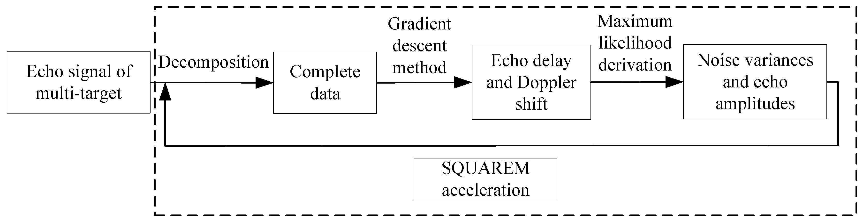
2.2. Stage 1: Delay-Doppler-SNR Estimation

In this section, a fast EM algorithm is proposed to estimate $\mathit{\psi }$. The proposed GAEM algorithm is illustrated in Figure 3.

2.2.1. Q function and Derivation of Complete Data

The log-likelihood of $Y_{lm}^q\left[u\right]$ is

$$\begin{array}{cc}\hfill lnp\left(Y_{lm}^q\left[u\right]\right)=& -ln\pi -ln{\sigma }_l^{q2}-\frac{1}{{\sigma }_l^{q2}}\hfill \\ \hfill & ·{\left|Y_{lm}^q\left[u\right]-\sqrt{\frac{E}{K}}\sum _{k=1}^K{\eta }_{lk}^q{S}_k\left[u\right]e^{-j2\pi u/N{f}_s{\tau }_{lk}^q-j2\pi m\mathrm{PRI}{f}_{lk}^q}\right|}^2.\hfill \end{array}$$

(13)

Let $\mathit{X}={\left[Y_{11}^1\left[1\right],\cdots ,Y_{LM}^{Q_0}\left[N\right]\right]}^T\in {\mathbb{C}}^{Q_{0}LMN\times 1}$, which denotes the complete data selected by the EM algorithm in this study, and we obtain

$$\begin{array}{cc}\hfill lnp\left(\mathit{X}\right)=& \sum _{l=1}^L\sum _{q=1}^{Q_0}\sum _{m=0}^{M-1}\sum _{u=0}^{N-1}lnp\left(Y_{lm}^q\left[u\right]\right)\hfill \\ \hfill =& const-MN\sum _{l=1}^L\sum _{q=1}^{Q_0}ln{\sigma }_l^{q2}-\sum _{l=1}^L\sum _{q=1}^{Q_0}\sum _{m=0}^{M-1}\sum _{u=0}^{N-1}\frac{1}{{\sigma }_l^{q2}}\hfill \\ \hfill & ·{\left|Y_{lm}^q\left[u\right]-\sqrt{\frac{E}{K}}\sum _{k=1}^K{\eta }_{lk}^q{S}_k\left[u\right]e^{-j2\pi u/N{f}_s{\tau }_{lk}^q-j2\pi m\mathrm{PRI}{f}_{lk}^q}\right|}^2.\hfill \end{array}$$

(14)

According to the definition of the Q function in the EM algorithm, the Q function of the $(i+1)$th iteration is

$$\mathrm{Q}\left(\mathit{\psi },{\mathit{\psi }}^{\left(i\right)}\right)=E_{\mathit{X}}\left[\left.lnp\left(\mathit{X}\right)\right|\mathit{Y},{\mathit{\psi }}^{\left(i\right)}\right],$$

(15)

where $E_{\mathit{X}}\left[·\right]$ represents the expectation of the formula with respect to the random vector $\mathit{X}$. ${\mathit{\psi }}^{\left(i\right)}$ in (15) denotes the estimated result of the ith iteration, which is known in the $(i+1)$th iteration. The parameters to be estimated in the Q function here are echo delay/Doppler shift $\mathit{\gamma }$, echo amplitude $\mathit{\eta }$ and noise variance ${\mathit{\sigma }}^2$.

Substituting (14) into (15), we can get

$$\begin{array}{cc}\hfill \mathrm{Q}\left(\mathit{\psi },{\mathit{\psi }}^{\left(i\right)}\right)=& const-MN\sum _{l=1}^L\sum _{q=1}^{Q_0}ln{\sigma }_l^{q2}\hfill \\ \hfill & -\sum _{l=1}^L\sum _{q=1}^{Q_0}\sum _{m=0}^{M-1}\sum _{u=0}^{N-1}\frac{1}{{\sigma }_l^{q2}}\left\{E_{\mathit{X}}\left[\left.{\left|Y_{lm}^q\left[u\right]\right|}^2\right|Y_{lm}\left[u\right],{\mathit{\psi }}^{\left(i\right)}\right]\right.\hfill \\ \hfill & \left.-2\mathrm{Re}\left\{{\left(A_{lm}^q\left[u\right]\right)}^{*}{E}_{\mathit{X}}\left[\left.Y_{lm}^q\left[u\right]\right|Y_{lm}\left[u\right],{\mathit{\psi }}^{\left(i\right)}\right]\right\}+{\left|A_{lm}^q\left[u\right]\right|}^2\right\},\hfill \end{array}$$

(16)

where

$$A_{lm}^q\left[u\right]=\sqrt{\frac{E}{K}}\sum _{k=1}^K{\eta }_{lk}^q{S}_k\left[u\right]e^{-j2\pi u/N{f}_s{\tau }_{lk}^q-j2\pi m\mathrm{PRI}{f}_{lk}^q},$$

(17)

$$\begin{array}{cc}\hfill E_{\mathit{X}}\left[\left.{\left|Y_{lm}^q\left[u\right]\right|}^2\right|Y_{lm}\left[u\right],{\mathit{\psi }}^{\left(i\right)}\right]=& {\sigma }_l^{q2\left(i\right)}-\frac{{\left({\sigma }_l^{q2\left(i\right)}\right)}^2}{{\sigma }_l^{2\left(i\right)}}+{\left(E_{\mathit{X}}\left[\left.Y_{lm}^q\left[u\right]\right|Y_{lm}\left[u\right],{\mathit{\psi }}^{\left(i\right)}\right]\right)}^{*}\hfill \\ \hfill & ·E_{\mathit{X}}\left[\left.Y_{lm}^q\left[u\right]\right|Y_{lm}\left[u\right],{\mathit{\psi }}^{\left(i\right)}\right],\hfill \end{array}$$

(18)

$$\begin{array}{cc}\hfill E_{\mathit{X}}\left[\left.Y_{lm}^q\left[u\right]\right|Y_{lm}\left[u\right],{\mathit{\psi }}^{\left(i\right)}\right]=& \sqrt{\frac{E}{K}}\sum _{k=1}^K{\eta }_{lk}^{q\left(i\right)}{S}_k\left[u\right]e^{-j2\pi u/N{f}_s{\tau }_{lk}^{q\left(i\right)}-j2\pi m\mathrm{PRI}{f}_{lk}^{q\left(i\right)}}+\frac{{\sigma }_l^{q2\left(i\right)}}{{\sigma }_l^{2\left(i\right)}}\hfill \\ \hfill & ·\left(Y_{lm}\left[u\right]-\sqrt{\frac{E}{K}}\sum _{q=1}^{Q_0}\sum _{k=1}^K{\eta }_{lk}^{q\left(i\right)}{S}_k\left[u\right]e^{-j2\pi u/N{f}_s{\tau }_{lk}^{q\left(i\right)}-j2\pi m\mathrm{PRI}{f}_{lk}^{q\left(i\right)}}\right).\hfill \end{array}$$

(19)

${\left(·\right)}^{*}$ in (16) and (18) means complex conjugate. ${\sigma }_l^{2\left(i\right)}$ in (18) and (19) satisfies ${\sigma }_l^{2\left(i\right)}={\sum }_{q=1}^{Q_0}{\sigma }_l^{q2\left(i\right)}$. For simplicity, $E_{\mathit{X}}\left[\left.Y_{lm}^q\left[u\right]\right|Y_{lm}\left[u\right],{\mathit{\psi }}^{\left(i\right)}\right]$ is denoted by ${\tilde{Y}}_{lm}^q\left[u\right]$. We define $\tilde{\mathit{X}}=\left[{\tilde{Y}}_{11}^1\left[1\right],\cdots \right.$${\left.,{\tilde{Y}}_{LM}^{Q_0}\left[N\right]\right]}^T\in {\mathbb{C}}^{Q_{0}LMN\times 1}$. By substituting (18) into (16), the Q function can be reformulated as

$$\begin{array}{cc}\hfill \mathrm{Q}\left(\mathit{\psi },{\mathit{\psi }}^{\left(i\right)}\right)=& const-MN\sum _{l=1}^L\sum _{q=1}^{Q_0}ln{\sigma }_l^{q2}-\sum _{l=1}^L\sum _{q=1}^{Q_0}\sum _{m=0}^{M-1}\sum _{u=0}^{N-1}\frac{1}{{\sigma }_l^{q2}}\left\{{\sigma }_l^{q2\left(i\right)}-\frac{{\left({\sigma }_l^{q2\left(i\right)}\right)}^2}{{\sigma }_l^{2\left(i\right)}}\right.\hfill \\ \hfill & \left.+{\left|{\tilde{Y}}_{lm}^q\left[u\right]-\sqrt{\frac{E}{K}}\sum _{k=1}^K{\eta }_{lk}^q{S}_k\left[u\right]e^{-j2\pi u/N{f}_s{\tau }_{lk}^q-j2\pi m\mathrm{PRI}{f}_{lk}^q}\right|}^2\right\}.\hfill \end{array}$$

(20)

Unlike the use of the EM algorithm to estimate the parameters of the superimposed targets in [15], this study extends the parameters to be estimated of the Q function in the EM algorithm, where the echo amplitude $\mathit{\eta }$ and noise variance ${\mathit{\sigma }}^2$ are estimated in each iteration of EM algorithm. The estimations of echo amplitude $\mathit{\eta }$ and noise variance ${\mathit{\sigma }}^2$ conform to the actual scenario of SNR fluctuations in different propagation paths of the MIMO radar, which ensures the accuracy of multi-target parameter estimation results.

2.2.2. Estimation of Parameters in SNR

Since the signals transmitted from different radar nodes are assumed to be orthogonal, we obtain

$$\begin{array}{cc}\hfill & \sum _{u=0}^{N-1}{\left|\sqrt{\frac{E}{K}}\sum _{k=1}^K{\eta }_{lk}^q{S}_k\left[u\right]e^{-j2\pi u/N{f}_s{\tau }_{lk}^q-j2\pi m\mathrm{PRI}{f}_{lk}^q}\right|}^2\hfill \\ \hfill & =\sum _{k=1}^K\frac{E}{K}{\left|{\eta }_{lk}^q\right|}^2\sum _{u=0}^{N-1}{\left|S_k\left[u\right]\right|}^2=\frac{E}{K}N{f}_s\sum _{k=1}^K{\left|{\eta }_{lk}^q\right|}^2.\hfill \end{array}$$

(21)

Based on (20) and (21), the maximum likelihood (ML) estimator of ${\eta }_{lk}^q$ is given as

$$\begin{array}{cc}\hfill {\widehat{\eta }}_{lk}^q=& \underset{{\eta }_{lk}^q}{argmax}\left\{\sum _{l=1}^L\sum _{q=1}^{Q_0}\sum _{m=0}^{M-1}\sum _{u=0}^{N-1}\frac{1}{{\sigma }_l^{q2}}2\mathrm{Re}\left\{{\left({\tilde{Y}}_{lm}^q\left[u\right]\right)}^{*}\sqrt{\frac{E}{K}}\sum _{k=1}^K{\eta }_{lk}^q\right.\right.\hfill \\ \hfill & ·\left.\left.S_k\left[u\right]e^{-j2\pi u/N{f}_s{\tau }_{lk}^q-j2\pi m\mathrm{PRI}{f}_{lk}^q}\right\}-\frac{E}{K}MN{f}_s\sum _{l=1}^L\sum _{q=1}^{Q_0}\sum _{k=1}^K\frac{1}{{\sigma }_l^{q2}}{\left|{\eta }_{lk}^q\right|}^2\right\}.\hfill \end{array}$$

(22)

By taking the partial differentiation of the formula in $argmax\left\{·\right\}$ with respect to ${\eta }_{lk}^q$ and setting the derivative equal to zero, the explicit expression of the ML estimate ${\widehat{\eta }}_{lk}^q$ can be written as

$${\widehat{\eta }}_{lk}^q=\frac{1}{MN{f}_s}\sum _{m=0}^{M-1}\sum _{u=0}^{N-1}{\tilde{Y}}_{lm}^q\left[u\right]\sqrt{\frac{K}{E}}{S}_k^{*}\left[u\right]e^{j2\pi u/N{f}_s{\tau }_{lk}^q+j2\pi m\mathrm{PRI}{f}_{lk}^q}.$$

(23)

Equation (20) can be simplified based on (21). Next, by substituting (23) into simplified (20), it can be seen from (8) that we can change $\mathit{\psi }$ in (20) into $\left[\mathit{\gamma };{\mathit{\sigma }}^2\right]$, thus obtaining a new Q function, which is named as ${\mathrm{Q}}_1$ in this paper, as shown below:

$$\begin{array}{cc}\hfill {\mathrm{Q}}_1\left(\left[\mathit{\gamma };{\mathit{\sigma }}^2\right],{\mathit{\psi }}^{\left(i\right)}\right)=& const-MN\sum _{l=1}^L\sum _{q=1}^{Q_0}ln{\sigma }_l^{q2}-\sum _{l=1}^L\sum _{q=1}^{Q_0}\sum _{m=0}^{M-1}\sum _{u=0}^{N-1}\frac{1}{{\sigma }_l^{q2}}\hfill \\ \hfill & ·\left\{{\sigma }_l^{q2\left(i\right)}-\frac{{\left({\sigma }_l^{q2\left(i\right)}\right)}^2}{{\sigma }_l^{2\left(i\right)}}+{\left|{\tilde{Y}}_{lm}^q\left[u\right]\right|}^2\right\}+\sum _{l=1}^L\sum _{q=1}^{Q_0}\sum _{k=1}^K\frac{1}{{\sigma }_l^{q2}}\frac{1}{MN{f}_s}\hfill \\ \hfill & ·{\left|\sum _{u=0}^{N-1}\sum _{m=0}^{M-1}{\left({\tilde{Y}}_{lm}^q\left[u\right]\right)}^{*}{S}_k\left[u\right]e^{-j2\pi u/N{f}_s{\tau }_{lk}^q-j2\pi m\mathrm{PRI}{f}_{lk}^q}\right|}^2.\hfill \end{array}$$

(24)

Since the derivation of (24) involves the estimation of ${\eta }_{lk}^q$, and the parameter estimation accuracy is affected by the SNR, (24) is an approximation of (20). By taking the partial derivative of (24) with respect to ${\sigma }_l^{q2}$ and setting the derivative equal to zero, the explicit expression for the ML estimate ${\widehat{\sigma }}_l^{q2}$ is obtained as

$$\begin{array}{cc}\hfill {\widehat{\sigma }}_l^{q2}=& \frac{1}{MN}\left\{\sum _{m=0}^{M-1}\sum _{u=0}^{N-1}\left\{{\sigma }_l^{q2\left(i\right)}-{\left({\sigma }_l^{q2\left(i\right)}\right)}^2/{\sigma }_l^{2\left(i\right)}+{\left|{\tilde{Y}}_{lm}^q\left[u\right]\right|}^2\right\}\right.\hfill \\ \hfill & \left.-\sum _{k=1}^K\frac{1}{MN{f}_s}{\left|\sum _{u=0}^{N-1}\sum _{m=0}^{M-1}{\left({\tilde{Y}}_{lm}^q\left[u\right]\right)}^{*}{S}_k\left[u\right]e^{-j2\pi u/N{f}_s{\tau }_{lk}^q-j2\pi m\mathrm{PRI}{f}_{lk}^q}\right|}^2\right\}.\hfill \end{array}$$

(25)

Now, the explicit expression for the ML estimate ${\widehat{\eta }}_{lk}^q$ and ${\widehat{\sigma }}_l^{q2}$ are derived.

2.2.3. Echo Delay and Doppler Shift Estimation

Substituting (25) into (24), we simplify $\left[\mathit{\gamma };{\mathit{\sigma }}^2\right]$ in (24) to $\mathit{\gamma }$, and ${\mathrm{Q}}_1$ is updated and named as ${\mathrm{Q}}_2$:

$$\begin{array}{cc}\hfill {\mathrm{Q}}_2\left(\mathit{\gamma },{\mathit{\psi }}^{\left(i\right)}\right)=& cons{t}_2-MN\sum _{l=1}^L\sum _{q=1}^{Q_0}ln\left\{\frac{1}{MN}\left\{\sum _{m=0}^{M-1}\sum _{u=0}^{N-1}\right.\right.\hfill \\ \hfill & \left\{{\sigma }_l^{q2\left(i\right)}-{\left({\sigma }_l^{q2\left(i\right)}\right)}^2/{\sigma }_l^{2\left(i\right)}+{\left|{\tilde{Y}}_{lm}^q\left[u\right]\right|}^2\right\}-\sum _{k=1}^K\frac{1}{MN{f}_s}\hfill \\ \hfill & \left.\left.·{\left|\sum _{u=0}^{N-1}\sum _{m=0}^{M-1}{\left({\tilde{Y}}_{lm}^q\left[u\right]\right)}^{*}{S}_k\left[u\right]e^{-j2\pi u/N{f}_s{\tau }_{lk}^q-j2\pi m\mathrm{PRI}{f}_{lk}^q}\right|}^2\right\}\right\}.\hfill \end{array}$$

(26)

Similar to the derivation of ${\mathrm{Q}}_1$, compared with (24), the derivation process of (26) includes the estimation of ${\sigma }_l^{q2}$. The parameter estimation accuracy will be affected by the SNR, so (26) is an approximation of (24). Since ${\sigma }_l^{q2\left(i\right)}$, ${\sigma }_l^{2\left(i\right)}$, and ${\tilde{Y}}_{lm}^q\left[u\right]$ in (26) are composed of the estimation results of the ith iteration or echo data, the echo delay and Doppler parameter vector $\mathit{\gamma }$ can be estimated by the following optimization criterion:

$$\begin{array}{cc}\hfill \widehat{\mathit{\gamma }}=& \underset{\mathit{\gamma }}{argmax}\left({\mathrm{Q}}_2\left(\mathit{\gamma },{\mathit{\psi }}^{\left(i\right)}\right)\right)\hfill \\ \hfill =& \underset{\mathit{\gamma }}{argmax}\left\{{\left|\sum _{u=0}^{N-1}\sum _{m=0}^{M-1}{\left({\tilde{Y}}_{lm}^q\left[u\right]\right)}^{*}{S}_k\left[u\right]e^{-j2\pi u/N{f}_s{\tau }_{lk}^q-j2\pi m\mathrm{PRI}{f}_{lk}^q}\right|}^2\right\}.\hfill \end{array}$$

(27)

For one $kql$th propagation path, the dimension of $\mathit{\gamma }$ can be reduced to 2. Then, we can draw an objective function of (27) as below:

From Figure 4, we can find the objective function is convex when the distance varies from 3970 m to 4030 m and the speed varies from 0 m/s to 10 m/s. Hence, different from the traditional grid point search method, this study employs the gradient descent algorithm to solve the echo delay and Doppler shift. That is, instead of computing the maximizer of ${\mathrm{Q}}_2\left(·,{\mathit{\psi }}^{\left(i\right)}\right)$, we can find a vector ${\mathit{\gamma }}^{\left(i+1\right)}$ that satisfies ${\mathrm{Q}}_2\left({\mathit{\gamma }}^{\left(i+1\right)},{\mathit{\psi }}^{\left(i\right)}\right)\ge {\mathrm{Q}}_2\left({\mathit{\gamma }}^{\left(i\right)},{\mathit{\psi }}^{\left(i\right)}\right)$ (i.e., an improvement). This is conducive for reducing the computational complexity of each M-step in EM algorithm.

To achieve ${\mathrm{Q}}_2\left({\mathit{\gamma }}^{\left(i+1\right)},{\mathit{\psi }}^{\left(i\right)}\right)\ge {\mathrm{Q}}_2\left({\mathit{\gamma }}^{\left(i\right)},{\mathit{\psi }}^{\left(i\right)}\right)$, one iterative gradient algorithm can be formulated as

$${\mathit{\gamma }}^{\left(i+1\right)}={\mathit{\gamma }}^{\left(i\right)}+\mu \left[{\left.{\nabla }_{\mathit{\gamma }}{\mathrm{Q}}_2\left(\mathit{\gamma },{\mathit{\psi }}^{\left(i\right)}\right)\right|}_{\mathit{\gamma }={\mathit{\gamma }}^{\left(i\right)}}\right],$$

(28)

where $\mu$ is the step size that depends on ${\left.{\nabla }_{\mathit{\gamma }}{\mathrm{Q}}_2\left(\mathit{\gamma },{\mathit{\psi }}^{\left(i\right)}\right)\right|}_{\mathit{\gamma }={\mathit{\gamma }}^{\left(i\right)}}$.

So far, the delay, Doppler and parameters related to SNR are estimated. In addition, we provide a computational complexity analysis in terms of complex multiplications here. In the traditional EM algorithm, the computational time of the algorithm is mainly spent in solving (27). For the grid point search method, it requires approximately $O\left(LK{Q}_{0}MN{M}_1{N}_1\right)$ operations, where $M_1$ and $N_1$ denote the search points of the Doppler and echo delay, respectively. Moreover, the estimation precision of the delay and Doppler is restricted by the grid interval. That is, for the grid point search method, the computational complexity must be increased to improve the estimation accuracy. For the GAEM algorithm in this study, since the gradient descent algorithm is used to solve (27), each iteration requires approximately $O\left(LK{Q}_{0}MN\right)$ operations. In addition, the convergence of GAEM algorithm can be achieved in a finite number of iterations. Therefore, compared with the traditional EM algorithm, the GAEM algorithm proposed in this study is faster.

The entire flow of the GAEM algorithm is summarized as Algorithm 1. Steps 4∼8 are set in Algorithm 1 as an iteration of the GAEM algorithm. Based on [24], the squared iterative methods (SQUAREM) algorithm is adopted in this study to minimize the number of iterations of the GAEM algorithm.

Algorithm 1 GAEM algorithm

Input:  $\mathit{Y}$ Output:  $\widehat{\mathit{\psi }}$ 1: Initialize ${\mathit{\psi }}^{\left(1\right)}$; 2: $i=1$; 3: repeat 4:    Decompose the echo data $\mathit{Y}$ into complete data $\tilde{\mathit{X}}$ according to (19) and ${\mathit{\psi }}^{\left(i\right)}$; 5:    Calculate ${\mathit{\gamma }}^{\left(i+1\right)}$ according to (28) and $\tilde{\mathit{X}}$; 6:    Compute ${\mathit{\sigma }}^{2\left(i+1\right)}$ according to (25), (9), $\tilde{\mathit{X}}$, ${\mathit{\psi }}^{\left(i\right)}$, and ${\mathit{\gamma }}^{\left(i+1\right)}$; 7:    Compute ${\mathit{\eta }}^{\left(i+1\right)}$ according to (23), (9), $\tilde{\mathit{X}}$, and ${\mathit{\gamma }}^{\left(i+1\right)}$; 8:    Collect ${\mathit{\gamma }}^{\left(i+1\right)}$, ${\mathit{\sigma }}^{2\left(i+1\right)}$, and ${\mathit{\eta }}^{\left(i+1\right)}$ in ${\mathit{\psi }}^{\left(i+1\right)}$ according to (8); 9:    Substitute ${\mathit{\psi }}^{\left(i+1\right)}$ into (20) to determine convergence; 10:    $i=i+1$; 11: until convergence 12: $\widehat{\mathit{\psi }}={\mathit{\psi }}^{\left(i\right)}$;

The entire flow of the combination of GAEM algorithm and SQUAREM is summarized as Algorithm 2, which is shown at top of next page. The $\mathrm{GAEMupdate}\left(·\right)$ in Algorithm 2 is an iteration of the GAEM algorithm. According to Algorithm 2, the computational complexity of the GAEM algorithm accelerated by SQUAREM is $O\left(3LK{Q}_{0}MN+5LK{Q}_0\right)\approx O\left(LK{Q}_{0}MN\right)$. That is, the computational complexity of the algorithm does not increase significantly after combining with SQUAREM.

Algorithm 2 GAEM+SQUAREM algorithm

Input:  $\mathit{Y}$ Output:  $\widehat{\mathit{\psi }}$ 1: Initialize ${\mathit{\psi }}^{\left(1\right)}$; 2: $i=1$; 3: repeat 4:    ${\mathit{\psi }}^{\left(i+1\right)}=\mathrm{GAEMupdate}\left({\mathit{\psi }}^{\left(i\right)}\right)$; 5:    ${\mathit{\psi }}^{\left(i+2\right)}=\mathrm{GAEMupdate}\left({\mathit{\psi }}^{\left(i+1\right)}\right)$; 6:    $\mathit{r}={\mathit{\psi }}^{\left(i+1\right)}-{\mathit{\psi }}^{\left(i\right)}$ 7:    $\mathit{v}=\left({\mathit{\psi }}^{\left(i+2\right)}-{\mathit{\psi }}^{\left(i+1\right)}\right)-\mathit{r}$ 8:    $\rho =-\frac{{∥\mathit{r}∥}_2}{{∥\mathit{v}∥}_2}$ 9:    ${\mathit{\psi }}^{\left(i+3\right)}={\mathit{\psi }}^{\left(i\right)}-2\mathit{\rho }\mathit{r}+{\mathit{\rho }}^2\mathit{v}$; 10:    ${\mathit{\psi }}^{\left(i+4\right)}=\mathrm{GAEMupdate}\left({\mathit{\psi }}^{\left(i+3\right)}\right)$; 11:    Substitute ${\mathit{\psi }}^{\left(i+4\right)}$ into (20) to determine convergence; 12:    $i=i+4$; 13: until convergence 14: $\widehat{\mathit{\psi }}={\mathit{\psi }}^{\left(i\right)}$;

2.3. Stage 2: Target Parameters and System Deviations Estimation

The estimated echo delay and Doppler in Section 2.2 is denoted by the vector $\widehat{\mathit{\gamma }}$. Since the GAEM algorithm proposed in this paper is essentially an ML algorithm, the ML estimate $\widehat{\mathit{\gamma }}$ is asymptotically distributed according to $\mathcal{N}\left(\mathit{\gamma },{\mathbf{J}}_{\gamma }^{-1}\right)$. ${\mathbf{J}}_{\gamma }$ represents the Fisher information matrix (FIM) of $\widehat{\mathit{\gamma }}$. Section 2.4 derives the expression of ${\mathbf{J}}_{\gamma }$ and the SNR required to calculate ${\mathbf{J}}_{\gamma }$ are estimated in Section 2.2.2.

Let $\mathit{\gamma }=g\left(\mathit{\alpha }\right)$. Due to the asymptotic statistical property of $\widehat{\mathit{\gamma }}$, the estimator of target parameters and system deviations is $\underset{\mathit{\alpha }}{argmin}{\left(\widehat{\mathit{\gamma }}-g\left(\mathit{\alpha }\right)\right)}^T{\mathbf{J}}_{\gamma }\left(\widehat{\mathit{\gamma }}-g\left(\mathit{\alpha }\right)\right)$, which can be reformulated as

$$\underset{\mathit{\alpha }}{argmin}{∥\sqrt{{\mathbf{J}}_{\gamma }}\widehat{\mathit{\gamma }}-\sqrt{{\mathbf{J}}_{\gamma }}g\left(\mathit{\alpha }\right)∥}_2^2.$$

(29)

Equation (29) can be solved as follows. Let $\sqrt{{\mathbf{J}}_{\gamma }}{\mathit{\gamma }}_i=\sqrt{{\mathbf{J}}_{\gamma }}g\left({\mathit{\alpha }}_i\right)$ and $\sqrt{{\mathbf{J}}_{\gamma }}\widehat{\mathit{\gamma }}=\sqrt{{\mathbf{J}}_{\gamma }}g\left({\mathit{\alpha }}_{i+1}\right)$, where ${\mathit{\alpha }}_i$ is the result of the ith iteration. Then, a Taylor series expansion of $\sqrt{{\mathbf{J}}_{\gamma }}g\left({\mathit{\alpha }}_{i+1}\right)$ around ${\mathit{\alpha }}_i$ is given as

$$\begin{array}{cc}\hfill \sqrt{{\mathbf{J}}_{\gamma }}\widehat{\mathit{\gamma }}=& \sqrt{{\mathbf{J}}_{\gamma }}{\mathit{\gamma }}_{i+1}\hfill \\ \hfill \approx & \sqrt{{\mathbf{J}}_{\gamma }}g\left({\mathit{\alpha }}_i\right)+\sqrt{{\mathbf{J}}_{\gamma }}{\left.\frac{\partial g\left(\mathit{\alpha }\right)}{\partial \mathit{\alpha }}\right|}_{\mathit{\alpha }={\mathit{\alpha }}_i}\left({\mathit{\alpha }}_{i+1}-{\mathit{\alpha }}_i\right).\hfill \end{array}$$

(30)

Set ${\left.\frac{\partial g\left(\mathit{\alpha }\right)}{\partial \mathit{\alpha }}\right|}_{\mathit{\alpha }={\mathit{\alpha }}_i}={\mathbf{P}}_i$. Then, we have

$${\mathit{\alpha }}_{i+1}={\left({\mathbf{P}}_i^T{\mathbf{J}}_{\gamma }{\mathbf{P}}_i\right)}^{-1}{\mathbf{P}}_i^T{\mathbf{J}}_{\gamma }\left[\widehat{\mathit{\gamma }}-g\left({\mathit{\alpha }}_i\right)\right]+{\mathit{\alpha }}_i.$$

(31)

Based on (29), a rough estimation result of the target position/velocity can be calculated when the radar system deviation is set to $\mathbf{0}$. The rough estimation result of the target position/velocity and the zero system deviation are integrated into the initial value ${\mathit{\alpha }}_0$ of (31).

At this point, a robust and fast self-calibration algorithm is realized. Robustness implies that the algorithm can be applied to non-ideal scenarios such as superimposed signals and SNR fluctuations. Quickness implies that we reduce not only the computational complexity within each iteration of the EM algorithm, but also the overall number of iterations of the EM algorithm.

2.4. Cramér-Rao Bound in the Non-Ideal Environment

From the definition of CRB [31], we can get

$$\mathrm{CRB}\left(\mathit{\vartheta }\right)=\mathbf{J}{\left(\mathit{\vartheta }\right)}^{-1}=-{\mathrm{E}}_{\mathit{y}}\left[\frac{{\partial }^{2}ln\mathrm{p}\left(\mathit{y};\mathit{\vartheta }\right)}{\partial \mathit{\vartheta }\partial {\mathit{\vartheta }}^{\mathrm{T}}}\right].$$

(32)

Using the chain rule,

$$\begin{array}{cc}\hfill \mathbf{J}\left(\mathit{\vartheta }\right)=& \left[\begin{array}{cc}{\mathbf{P}}^T& \\ & {\mathbf{I}}_{2LK{Q}_0+L{Q}_0}\end{array}\right]\mathbf{J}\left(\mathit{\psi }\right)\left[\begin{array}{cc}\mathbf{P}& \\ & {\mathbf{I}}_{2LK{Q}_0+L{Q}_0}\end{array}\right],\hfill \end{array}$$

(33)

$${\left[\mathbf{P}\right]}_{ij}=\frac{\partial {\left[\mathit{\gamma }\right]}_i}{\partial {\left[\mathit{\alpha }\right]}_j},\mathbf{J}\left(\mathit{\psi }\right)=-E_{\mathit{y}}\left[\frac{{\partial }^{2}lnp\left(\mathit{y};\mathit{\psi }\right)}{\partial \mathit{\psi }\partial {\mathit{\psi }}^T}\right].$$

(34)

From the derivation of [32],

$${\left[\mathbf{J}\left(\mathit{\psi }\right)\right]}_{ij}=\mathrm{tr}\left[{\mathbf{G}}^{-1}\left(\mathit{\psi }\right)\frac{\partial \mathbf{G}\left(\mathit{\psi }\right)}{\partial {\left[\mathit{\psi }\right]}_i}{\mathbf{G}}^{-1}\left(\mathit{\psi }\right)\frac{\partial \mathbf{G}\left(\mathit{\psi }\right)}{\partial {\left[\mathit{\psi }\right]}_j}\right]+2\mathrm{Re}\left[\frac{\partial {\mathit{\mu }}^H\left(\mathit{\psi }\right)}{\partial {\left[\mathit{\psi }\right]}_i}{\mathbf{G}}^{-1}\left(\mathit{\psi }\right)\frac{\partial \mathit{\mu }\left(\mathit{\psi }\right)}{\partial {\left[\mathit{\psi }\right]}_j}\right],$$

(35)

$$\mathbf{G}\left(\mathit{\psi }\right)=\left[\begin{array}{ccc}{\left({\sigma }_{w1}\right)}^2{\mathbf{I}}_{NM}& & \\ & \ddots & \\ & & {\left({\sigma }_{wL}\right)}^2{\mathbf{I}}_{NM}\end{array}\right]\in {\mathbb{R}}^{LNM\times LNM},$$

(36)

$$\begin{array}{cc}\hfill \mathit{\mu }\left(\mathit{\psi }\right)=& \sqrt{\frac{E}{K}}\left[\sum _{q=1}^{Q_0}\sum _{k=1}^K{\eta }_{1k}^q{s}_k\left(0;{\tau }_{1k}^q\right),\dots \right.\hfill \\ \hfill & {\left.,\sum _{q=1}^{Q_0}\sum _{k=1}^K{\eta }_{Lk}^q{s}_k\left(N-1;{\tau }_{Lk}^q\right)e^{-j2\pi \left(M-1\right)\mathrm{PRI}{f}_{Lk}^q}\right]}^T\in {\mathbb{R}}^{LNM\times 1}.\hfill \end{array}$$

(37)

The elements of $\mathbf{J}\left(\mathit{\psi }\right)$ are calculated in Appendix A. ${\left({\sigma }_{wl}\right)}^2$ in (36) is the variance of Gaussian noise $w_{lm}\left[n\right]$. Based on the definition of Section 2.1, ${\varsigma }_{lm}\left[u\right]$ is the Fourier transform of $w_{lm}\left[n\right]$, and ${\left({\sigma }_l\right)}^2$ is the variance of Gaussian noise ${\varsigma }_{lm}\left[u\right]$. From (7), the variances mentioned above have the following functional relationship:

$${\left({\sigma }_{wl}\right)}^2=\frac{1}{N}{\left({\sigma }_l\right)}^2=\frac{1}{N}\sum _{q=1}^{Q_0}{\left({\sigma }_l^q\right)}^2.$$

(38)

For clarity, $\mathbf{J}\left(\mathit{\psi }\right)$ is expressed as

$$\mathbf{J}\left(\mathit{\psi }\right)=\begin{array}{c}\hfill \left[\begin{array}{ccccc}{\mathbf{J}}_{\tau \tau }& {\mathbf{J}}_{\tau f}& {\mathbf{J}}_{\tau {\eta }_R}& {\mathbf{J}}_{\tau {\eta }_I}& \mathbf{0}\\ {\mathbf{J}}_{\tau f}^T& {\mathbf{J}}_{ff}& {\mathbf{J}}_{f{\eta }_R}& {\mathbf{J}}_{f{\eta }_I}& \mathbf{0}\\ {\mathbf{J}}_{\tau {\eta }_R}^T& {\mathbf{J}}_{f{\eta }_R}^T& {\mathbf{J}}_{{\eta }_R{\eta }_R}& {\mathbf{J}}_{{\eta }_R{\eta }_I}& \mathbf{0}\\ {\mathbf{J}}_{\tau {\eta }_I}^T& {\mathbf{J}}_{f{\eta }_I}^T& {\mathbf{J}}_{{\eta }_R{\eta }_I}^T& {\mathbf{J}}_{{\eta }_I{\eta }_I}& \mathbf{0}\\ \mathbf{0}& \mathbf{0}& \mathbf{0}& \mathbf{0}& {\mathbf{J}}_{\sigma \sigma }\end{array}\right]\end{array}=\begin{array}{c}\hfill \left[\begin{array}{cc}\mathbf{A}& \mathbf{B}\\ {\mathbf{B}}^T& \mathbf{C}\end{array}\right]\end{array}.$$

(39)

From the definition of Schur complement [33], ${\mathbf{J}}_{\gamma }$ proposed in Section 2.3 can be expressed as ${\mathbf{J}}_{\gamma }=\mathbf{A}-\mathbf{B}{\mathbf{C}}^{-1}{\mathbf{B}}^T$.

3. Results

In this section, the effectiveness of the proposed GAEM and WILS algorithm is verified by numerical simulations. In order to show the performance of the algorithm briefly, we define four radar nodes, and the distance between two radar nodes is 500 m. The angles of the four targets are $-{45}^{\circ }$, ${60}^{\circ }$, ${30}^{\circ }$ and ${35}^{\circ }$, respectively, and the distances between the four targets and first radar node is 2000 m, 2010 m, 2020 m and 2030 m, respectively. Both radar nodes and targets are moving.

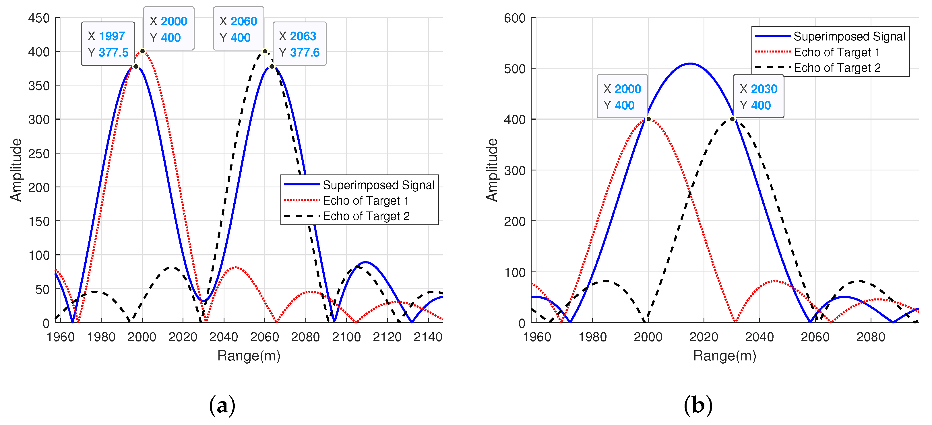
3.1. Estimation of Time Delay and Doppler

In this subsection, the SNR is 20 dB. The bandwidth of radar signal is 10 MHz, so the 3 dB width of the sinc function in the time domain is 15 m. However, the closest distance between targets is 10 m, which generates the superimposed signal. The simulation of the superimposed signal is shown in Figure 5.

Figure 5 shows the signal envelope in time domain after pulse compression. The dotted curve is the echo signal reflected from the first target. The dashed curve is the echo signal reflected from the second target. The solid curve is the superimposed signal of two targets. As can be seen from Figure 5a, when the distance between two targets is 60 m, the target distance corresponding to the superimposed signal peak is shifted from the real target distance. According to Figure 5b, when the distance between two targets is 30 m, the number of superimposed signal peaks becomes 1. The distance corresponding to the superimposed signal peak is still offset compared to the real target distance. Therefore, if the traditional ML algorithm is used to estimate the echo delay, the superimposed signals will affect the target parameter estimation.

The proposed GAEM is used to solve this problem. We compare GAEM algorithm with a gradient descent method based on traditional ML [34], and SQUAREM algorithm [24] is added to make GAEM converge faster. The root mean square error (RMSE) is used to evaluate the algorithm performance, as shown below

$$\mathrm{RMSE}=\sqrt{\frac{1}{MC}\sum _{m=1}^{MC}{\left(p_{esti}^{\left(m\right)}-p_{real}\right)}^2},$$

(40)

where MC represents the number of Monte Carlo simulations; $p_{esti}^{\left(m\right)}$ represents the estimated value; $p_{real}$ represents the real value.

Due to page limitations, only the delay and Doppler estimation results of the first target are shown. Figure 6 shows the RMSE of the estimation results against the number of iterations.

The line with square markers represents the echo delay estimate only using gradient descent algorithm. The line with diamond markers represents the echo delay estimate using GAEM algorithm proposed in this paper. It can be seen from the Figure 6a that GAEM algorithm is more robust than traditional “hill climbing” algorithm when the target echoes are superimposed. This is because compared with gradient descent, GAEM algorithm has E-step, that is, the adaptive decomposition of multi-target echoes based on the estimation results of the previous M-step. The line with square markers represents the estimation results after combining the proposed GAEM algorithm with SQUAREM algorithm. The simulation results indicate that the SQUAREM algorithm can further reduce the number of iterations of the GAEM algorithm. Figure 6b shows the estimation results of Doppler shift. The curve definition and conclusions in Figure 6b are consistent with those in Figure 6a.

The computational complexity curves versus the grid resolutions are depicted in Figure 7. According to Figure 7, the GAEM algorithm is much more efficient than the existing EM method.

3.2. Target Parameters and System Deviations Estimation

This subsection simulates the WILS algorithm proposed in Section 2.3. Since MIMO radar with widely separated antennas uses different radar nodes as receivers and has a large baseline, the noise variance and the echo coefficient in different propagation paths are considered to be different. In other words, the SNRs of signal echo in different propagation paths are different. In the simulation of this section, the SNRs of the three transmitting and three receiving radar nodes with the same target are set as ${\mathrm{SNR}}_0\left[0.01,0.6,1,0.8,0.02,1,0.4,0.06,1\right]$. The SNR mentioned in the simulation figures refers to the largest item (i.e., ${\mathrm{SNR}}_0$) in the above vector. When the SNR is 20 dB, the estimation results of target parameters and radar system deviations by GAEM and WILS algorithm are shown in Figure 8. Figure 8 is also the deployment of radar nodes and targets.

We compare the proposed WILS algorithm with the traditional LS algorithm [25], and add CRB simulation to show the performance of the proposed WILS algorithm. The simulation results of target parameter estimation are shown in Figure 9. The RMSE curves of WLIS algorithm are close to CRB curves. In contrast, the RMSE of the ILS algorithm lies above the CRB and the RMSE of the WILS algorithm. This is because the WILS algorithm adds the use of the SNR in different propagation paths, which ensures WILS has a more robust performance than ILS for non-ideal environment such as different noise variances of radar nodes and anisotropic targets. The noise variances and echo amplitudes are estimated in GAEM algorithm, which ensures the use of SNR in WILS algorithm.

The simulation results of radar system deviation estimation are shown in Figure 10. The conclusions of Figure 10 are identical to those in Figure 9a.

In summary, the proposed technique enables efficient and robust multi-target parameter estimation for MIMO radar with widely separated antennas on moving platforms.

4. Discussion

This paper deals with the problems of dense multi-target, SNR fluctuations of different propagation paths and high computational complexity of MIMO radar with widely separated antennas on moving platforms. In order to reduce the computational complexity, the gradient descent method is used to optimize the M-step in the EM algorithm. The simulation results indicate that the combination of the gradient descent and EM algorithm is feasible. Further, the echo amplitudes and noise variances are estimated and the WILS algorithm is used to ensure the robustness of the target parameter estimation algorithm. Moreover, the asymptotic property of the ML estimator ensures the realization of the notion that an echo with a high SNR should be assigned a large weight.

This study focuses on solving the practical problems encountered in the parameter estimation of MIMO radar with widely separated antennas on moving platforms. However, the work in this paper still has potential for further development. Firstly, inspired by Ref. [9], co-located MIMO antennas can be deployed in each platform. For this novel radar system, the advantages of both MIMO radar with widely separated antennas and co-located MIMO radar can be exploited, and waveform optimization can be used to further improve the performance of target parameter estimation. Secondly, for MIMO radar with widely separated antennas, target localization accuracy is affected by the topology of MIMO radar and targets [12]. MIMO radar with widely separated antennas on moving platforms naturally has the advantage of changing the radar topology in real time. How to optimize the radar topology configuration based on the estimated multi-target positions in this paper to further improve the target positioning accuracy is the area that needs to be studied in the future. Finally, it can be seen from [35] that when the number of parameters to be estimated is determined, adding more information will improve the estimation accuracy. Ref. [26] combines the target echo delay and direct wave delay to complete the estimation of radar system deviations. In the future, we can model the fast-time and slow-time of target echo and direct wave, and further improve the parameter estimation accuracy based on the increased direct wave information.

5. Conclusions

In this paper, a robust parameter estimation algorithm is proposed to achieve target localization in scenarios such as superimposed signals and SNR fluctuations of different propagation paths. Firstly, in order to estimate the echo delay/Doppler and SNR, this paper derives the Q function of EM algorithm. Secondly, in order to reduce the computational complexity of M-step in EM algorithm, the iterative gradient algorithm is used to realize the idea of the generalized EM algorithm. Furthermore, based on the estimation results of the previous method, the WILS algorithm is used to estimate the target positions and velocities. In addition, this paper deduces the CRB in the non-ideal environment. Finally, the simulation results verify the effectiveness of the algorithm proposed in this paper. Possible future works include the combination of MIMO radar with widely separated antennas and co-located MIMO radar, optimization of radar topology, and use of direct wave signals.

References

1. Ward, J. Space-Time Adaptive Processing for Airborne Radar; Number TR-1015; MIT Lincoln Laboratory: Lexington, MA, USA, 1994. [Google Scholar]
2. Chen, C.Y.; Vaidyanathan, P.P. MIMO Radar Space–Time Adaptive Processing Using Prolate Spheroidal Wave Functions. IEEE Trans. Signal Process. 2008, 56, 623–635. [Google Scholar] [CrossRef]
3. Cuomo, K.M.; Coutts, S.D.; McHarg, J.C.; Pulsone, N.B.; Robey, F.C. Wideband Aperture Coherence Processing for Next Generation Radar (NexGen); Number ESC-TR-2004-087; MIT Lincoln Laboratory: Lexington, MA, USA, 2004. [Google Scholar]
4. Zheng, H.; Jiu, B.; Li, K.; Liu, H. Joint Design of the Transmit Beampattern and Angular Waveform for Colocated MIMO Radar under a Constant Modulus Constraint. Remote Sens. 2021, 13, 3392. [Google Scholar] [CrossRef]
5. Li, J.; Stoica, P. MIMO Radar Signal Processing; Wiley: Hoboken, NJ, USA, 2009. [Google Scholar]
6. Haimovich, A.M.; Blum, R.S.; Cimini, L.J. MIMO Radar with Widely Separated Antennas. IEEE Signal Process. Mag. 2008, 25, 116–129. [Google Scholar] [CrossRef]
7. Lehmann, N.H.; Haimovich, A.M.; Blum, R.S.; Cimini, L. High Resolution Capabilities of MIMO Radar. In Proceedings of the 2006 Fortieth Asilomar Conference on Signals, Systems and Computers, Pacific Grove, CA, USA, 29 October–1 November 2006; pp. 25–30. [Google Scholar]
8. Li, H.; Wang, Z.; Liu, J.; Himed, B. Moving Target Detection in Distributed MIMO Radar on Moving Platforms. IEEE J. Sel. Top. Signal Process. 2015, 9, 1524–1535. [Google Scholar] [CrossRef]
9. Chen, P.; Zheng, L.; Wang, X.; Li, H.; Wu, L. Moving Target Detection Using Colocated MIMO Radar on Multiple Distributed Moving Platforms. IEEE Trans. Signal Process. 2017, 65, 4670–4683. [Google Scholar] [CrossRef]
10. He, Q.; Blum, R.S.; Godrich, H.; Haimovich, A.M. Target Velocity Estimation and Antenna Placement for MIMO Radar With Widely Separated Antennas. IEEE J. Sel. Top. Signal Process. 2010, 4, 79–100. [Google Scholar] [CrossRef]
11. Mitra, A.K. Position-adaptive UAV radar for urban environments. In Proceedings of the International Conference on Radar, Adelaide, SA, Australia, 3–5 September 2003; pp. 303–308. [Google Scholar] [CrossRef]
12. Godrich, H.; Haimovich, A.M.; Blum, R.S. Target localisation techniques and tools for multiple-input multiple-output radar. IET Radar Sonar Navig. 2009, 3, 314–327. [Google Scholar] [CrossRef]
13. He, Q.; Blum, R.S. Cramer–Rao Bound for MIMO Radar Target Localization With Phase Errors. IEEE Signal Process. Lett. 2010, 17, 83–86. [Google Scholar]
14. Lu, J.; Liu, F.; Liu, H.; Liu, Q. Target Localization Based on High Resolution Mode of MIMO Radar with Widely Separated Antennas. Remote Sens. 2022, 14, 902. [Google Scholar] [CrossRef]
15. Feder, M.; Weinstein, E. Parameter estimation of superimposed signals using the EM algorithm. IEEE Trans. Acoust. Speech Signal Process. 1988, 36, 477–489. [Google Scholar] [CrossRef] [Green Version]
16. Zhang, F.; Zhang, Z.; Yu, W. Direction of arrival estimation for the uniform or non-uniform noise with adaptive expectation maximisation algorithm. IET Radar Sonar Navig. 2020, 14, 1029–1038. [Google Scholar] [CrossRef]
17. Lu, L.; Wu, H.C. Robust Expectation–Maximization Direction-of-Arrival Estimation Algorithm for Wideband Source Signals. IEEE Trans. Veh. Technol. 2011, 60, 2395–2400. [Google Scholar] [CrossRef]
18. Lu, L.; Wu, H.C. Novel Robust Direction-of-Arrival-Based Source Localization Algorithm for Wideband Signals. IEEE Trans. Wirel. Commun. 2012, 11, 3850–3859. [Google Scholar] [CrossRef]
19. Mada, K.K.; Wu, H.C.; Iyengar, S.S. Efficient and Robust EM Algorithm for Multiple Wideband Source Localization. IEEE Trans. Veh. Technol. 2009, 58, 3071–3075. [Google Scholar] [CrossRef]
20. Frenkel, L.; Feder, M. Recursive expectation-maximization (EM) algorithms for time-varying parameters with applications to multiple target tracking. IEEE Trans. Signal Process. 1999, 47, 306–320. [Google Scholar] [CrossRef]
21. Chung, P.J.; Roberts, W.; Bohme, J. Recursive K-distribution parameter estimation. IEEE Trans. Signal Process. 2005, 53, 397–402. [Google Scholar] [CrossRef]
22. Chung, P.J.; Bohme, J. Comparative convergence analysis of EM and SAGE algorithms in DOA estimation. IEEE Trans. Signal Process. 2001, 49, 2940–2949. [Google Scholar] [CrossRef]
23. Chung, P.J.; Bohme, J. Recursive EM and SAGE-inspired algorithms with application to DOA estimation. IEEE Trans. Signal Process. 2005, 53, 2664–2677. [Google Scholar] [CrossRef]
24. Varadhan, R.; Roland, C. Simple and Globally Convergent Methods for Accelerating the Convergence of Any EM Algorithm. Scand. J. Stat. 2007, 35, 335–353. [Google Scholar] [CrossRef]
25. Li, Y.; Wang, X.; Ding, Z. Multi-Target Position and Velocity Estimation Using OFDM Communication Signals. IEEE Trans. Commun. 2020, 68, 1160–1174. [Google Scholar] [CrossRef]
26. Liang, J.; Leung, C.S.; So, H.C. Lagrange Programming Neural Network Approach for Target Localization in Distributed MIMO Radar. IEEE Trans. Signal Process. 2016, 64, 1574–1585. [Google Scholar] [CrossRef]
27. Yang, X.; Li, Y.; Sun, Y.; Long, T.; Sarkar, T.K. Fast and Robust RBF Neural Network Based on Global K-Means Clustering With Adaptive Selection Radius for Sound Source Angle Estimation. IEEE Trans. Antennas Propag. 2018, 66, 3097–3107. [Google Scholar] [CrossRef]
28. Ho, K.; Xu, W. An accurate algebraic solution for moving source location using TDOA and FDOA measurements. IEEE Trans. Signal Process. 2004, 52, 2453–2463. [Google Scholar] [CrossRef]
29. Ho, K.C.; Lu, X.; Kovavisaruch, L. Source Localization Using TDOA and FDOA Measurements in the Presence of Receiver Location Errors: Analysis and Solution. IEEE Trans. Signal Process. 2007, 55, 684–696. [Google Scholar] [CrossRef]
30. Liu, Y.; Liao, G.; Li, H.; Zhu, S.; Li, Y.; Yin, Y. Passive MIMO Radar Detection with Unknown Colored Gaussian Noise. Remote Sens. 2021, 13, 2708. [Google Scholar] [CrossRef]
31. Trees, H.L.V. Detection, Estimation, and Modulation Theory I; Prentice Hall: Hoboken, NJ, USA, 2001. [Google Scholar]
32. Kay, S.M. Fundamentals of Statistical Signal Processing: Estimation Theory; Prentice Hall: Hoboken, NJ, USA, 1993. [Google Scholar]
33. Stoica, P.; Simonyte, V.; Soderstrom, T. On the resolution performance of spectral analysis. Signal Process 1995, 44, 153–161. [Google Scholar] [CrossRef]
34. Chen, J.; Hudson, R.; Yao, K. Maximum-likelihood source localization and unknown sensor location estimation for wideband signals in the near-field. IEEE Trans. Signal Process. 2002, 50, 1843–1854. [Google Scholar] [CrossRef] [Green Version]
35. Schultheiss, P.; Weinstein, E. Lower bounds on the localization errors of a moving source observed by a passive array. IEEE Trans. Acoust. Speech Signal Process. 1981, 29, 600–607. [Google Scholar] [CrossRef]
Figure 1. System diagram of multiple-input multiple-output (MIMO) radar with widely separated antennas on moving platforms.
Remotesensing 14 01670 g001
Figure 2. Topology diagram of MIMO radar and targets, which shows two practical problems concerned in this paper: (1) target echo overlap, (2) different signal-to-noise ratios (SNRs) in different propagation paths.
Remotesensing 14 01670 g002
Figure 3. The generalized adaptive expectation maximization (GAEM) algorithm, which is accelerated by squared iterative methods (SQUAREM) algorithm.
Remotesensing 14 01670 g003
Figure 4. Objective function of echo delay and Doppler shift.
Remotesensing 14 01670 g004
Figure 5. Simulation of the superimposed signal. (a) The distance between two targets is 60 m. (b) The distance between two targets is 30 m.
Remotesensing 14 01670 g005
Figure 6. Estimation results for proposed GAEM and gradient descent method based on traditional maximum likelihood (ML) [34] in the presence of target echo superimposed. (a) Root mean square error (RMSE) for the echo delay estimation, (b) RMSE for the echo Doppler estimation.
Remotesensing 14 01670 g006
Figure 7. Computational complexity versus grid resolution for the GAEM and traditional EM.
Remotesensing 14 01670 g007
Figure 8. Deployment of radar nodes and targets.
Remotesensing 14 01670 g008
Figure 9. Estimation results for different methods in the presence of different SNRs in different propagation paths (a) RMSE for the DOA estimation, (b) RMSE for the target range estimation, (c) RMSE for the target tangential velocity estimation, (d) RMSE for the target radial velocity estimation.
Remotesensing 14 01670 g009
Figure 10. Estimation results for different methods in the presence of different SNRs in different propagation paths (a) RMSE for the radar position deviations estimation, (b) RMSE for the radar velocity deviations estimation.
Remotesensing 14 01670 g010
Publisher’s Note: MDPI stays neutral with regard to jurisdictional claims in published maps and institutional affiliations.