
A Self-Regulating Multi-Clutter Suppression Framework for Small Aperture HFSWR Systems

School of Electronics and Information Engineering, Harbin Institute of Technology, Harbin 150001, China
*
Author to whom correspondence should be addressed.
Remote Sens. 2022, 14(8), 1901; https://0-doi-org.brum.beds.ac.uk/10.3390/rs14081901
Submission received: 17 March 2022
/
Revised: 7 April 2022
/
Accepted: 11 April 2022
/
Published: 14 April 2022
(This article belongs to the Special Issue Sustained Ocean Surface Observation Using HF Radar: From Data to Societal Applications)
Abstract
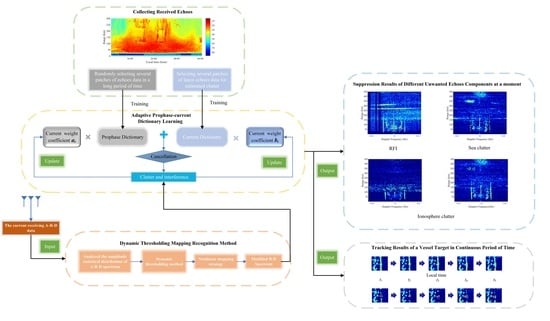
:The problem that this paper is concerned with is High Frequency Surface Wave Radar (HFSWR) detection of desired targets against a complex interference background consisting of sea clutter, ionosphere clutter, Radio Frequency Interference (RFI) and atmospheric noise. Eliminating unwanted echoes and exploring obscured targets contribute to achieving ideal surveillance of sea surface targets. In this paper, a Self-regulating Multi-clutter Suppression Framework (SMSF) has been proposed for small aperture HFSWR. SMSF can remove many types of clutter or RFI; meanwhile, it mines the targets merged into clutter and tracks the travelling path of the ship. In SMSF, a novel Dynamic Threshold Mapping Recognition (DTMR) method is first proposed to reduce the atmospheric noise and recognize each type of unwanted echo; these recognized echoes are fed into the proposed Adaptive Prophase-current Dictionary Learning (APDL) algorithm. To make a comprehensive evaluation, we also designed three novel assessment parameters: Obscured Targets Detection Rate (OTDR), Clutter Purification Rate (CPR) and Erroneous Suppression Rate (ESR). The experiment data collected from a small aperture HFSWR system confirm that SMSF has precise suppression performance over most of the classical algorithms and concurrently reveals the moving targets, and OTDR of SMSF is usually higher than compared methods.
1. Introduction
Because HFSWR provides the capability to receive target echoes over much longer distances than other traditional radars, such as microwave radars, it has been applied for surveilling the Exclusive Economic Zone (EEZ) and monitoring the sea state for many years. The HFSWR system performs in the lower part of the HF spectrum and is placed on the coastlines, using the electromagnetic coupling of radio waves to propagate signals along the sea surface. However, the transmitting antenna in the HFSWR system does not have perfect performance due to some limitations. A part of the radar signal propagates through the antenna sidelobes and points to the ionosphere. When the frequency of the radar signal is less than the critical frequency of the ionosphere, the radar signal could be backscattered to the receivers, thereby contaminating the echo signal [1]. Moreover, the ionospheric irregularities have a considerable effect upon the transmitting signals that propagate through them [2]. Initially, the ionosphere reflection coefficient was assumed to be a stochastic process with an associated spectral density function, which can explain the phase variations along the surface related to non-uniformity of the signal path [3]. Researchers mainly focused on signal processing techniques or designing adaptive receive antenna array. They also used ionosonde to observe the dynamic information of ionosphere clutter and collected sufficient data for designing radar parameters or confirming behavior rules of each layer in the ionosphere at different geographical locations [4,5]. Not long after, theoretical models of ionosphere clutter with different cases of reflection and deployment location could be presented for weakening the ionospheric clutter [6,7,8]. Space Time Adaptive Processing (STAP) techniques as a classical quantitative model can exploit the spatial properties of ionosphere clutter but it is difficult to collect adequate measured data for accurately estimating parameters [9]. Moreover, some methods used related transform approaches to explore different dimension features of targets and ionosphere clutter [10,11].
HFSWR has been successfully used for ocean remote sensing based on the first- and second-order monostatic radar cross-section models derived by Barrick [12] in the 1970s. Sea clutter as another severe problem also impacts the target detection in HFSWR systems operating on the shore-based or shipborne platform. Sea clutter can be defined as the backscattered returns from an area of sea surface illuminated by a transmitting signal. The Bragg lines are first-order scatters from surface waves, which have wavelength one half of the radar wavelength and move directly away or towards the receiving arrays. Generally, the power of Bragg lines is much stronger than the high-order sea clutter spectrum. When the current velocity at different directions is different, the first-order spectra have different offsets, thereby broadening the first-order spectrum [13]. The strong and broadened sea clutter may conceal the ship targets. Traditionally, sea clutter is viewed as a stochastic (random) process [14,15]. Over the past decade, the representative sea clutter suppression methods have included the subspace class method, Singular Value Decomposition (SVD) method, high-resolution method, modern spectral estimation method, the establishment of statistical distribution model and cyclic iterative cancellation method. Contrary to the aforementioned approaches, the recent booming development in deep learning opens up an elegant way of looking at the complex behavior of physical processes. In addition, it has resulted in a series of encouraging results in sea clutter suppression [16,17]. A lightweight deep convolutional learning network is established based on a Faster R-CNN and has been proposed for detecting the clutter region and interference [18].
Another interference factor is that the high spectrum is always occupied by other users, such as radio amateurs or radio stations, which may generate severe RFI. RFI in HFSWR systems has uniform spectral density over the receiver bandwidth and always occupies the entire range and Doppler domains [19]. Recently reported efforts on the RFI cancellation of HFSWR can be roughly divided into three types. The first type is based on space-time feature. Typically, according to the strong space correlation of small aperture array, robust adaptive beamforming methods using auxiliary beams have been developed [20,21]. The second one is based on subspace orthogonal projection, such as designing a Range-Doppler domain filter to suppress wideband RFI [22] or using the Higher-Order Singular Value Decomposition (HOSVD) to mine multidimensional structure information [23]. However, this type of method needs a large number of precise training samples. Third is the time-frequency analysis method, such as using inverse temporal windowing and Complex Empirical Mode Decomposition (CEMD) to mitigate the RFI [24] and employing the similarity constraint to design optimal filters or median detectors, which are suitable for nonhomogeneous environments [25,26]. It should be emphasized that some methods are ineffective due to wide beam and lack of polarization information in the small aperture HFSWR system. For example, the STAP method considers RFI to have an obvious directionality, which is in accord with the characteristic of large aperture array.
In order to obtain the ideal azimuth resolution, most existing HFSWR systems usually implement large receiving arrays, occupying hundreds or even thousands of meters for monitoring marine transportation. This design limits the flexibility of deploying the HFSWR system and greatly increases the manufacturing costs. The small aperture HFSWR as a burgeoning Over the Horizon Radar (OTHR) system requires less deployment space and lower manufacturing costs, and it is more appropriate for installing at the seashore due to covering less space. Hence, our team has dedicated ourselves to developing small aperture HFSWR for more than ten years and we have generally achieved inspiring advances. Several countries have also concentrated on developing the small aperture HFSWR system for many years. These systems are capable of detecting targets in the presence of backscatter from the surface of the Earth (either terrain or the sea), termed sea clutter and RFI from other users. Figure 1 presents the real scenario of coexistence of vessel targets, background noise, ionosphere clutter, sea clutter and ground clutter in an HFSWR RD image. The echoes data were collected at Weihai, China.
Most of the suppression methods only weaken one type of clutter contamination. Different kinds of clutter always concurrently appear in the actual operation. Hence, designing a novel suppression approach that can remove all kinds of undesired signals is urgently needed. Moreover, finding the targets merged into clutter or interference is a difficult task; a few existing studies focus on removing the clutter and simultaneously reserving obscured targets. Therefore, this paper is concerned with the perfection and improvement of the suppression clutter approach in two areas: first, removing many types of undesired components in the echo signal; second, finding out the targets obscured by clutter.
The main contributions are described as follows: the first one is designing a novel denoising process, DTMR, in the target detection. It realizes decontaminating RD images and recognizes each type of unwanted echo. Combining the deep learning and semi-empirical model to classify unwanted echo components, the data collection is more efficient and reliable. The second one is proposing an adaptive dictionary learning algorithm, which is a self-regulating dictionary according to current echoes. Certainly, it will exactly fit the varying clutter in various conditions. The third one is SMSF framework, which suppresses many types of clutter simultaneously, which is suitable for observing targets for a long period of time. The fourth one is proposed assessment parameters, Obscured Targets Detection Rate (OTDR), Clutter Purification Rate (CPR) and Erroneous Suppression Rate (ESR). This is the first instance of accessing suppression results by utilizing quantitative indicators and it can also be viewed as a more global approach to evaluate the performance of SMSF and other classical suppression methods.
The remainder of this article is organized as follows. Section 2 introduces some related algorithms and classical suppression methods, and also specifically introduces each step of the proposed framework, SMSF. Section 3 shows the experiment results and the suppression effect of SMSF. Section 4 thoroughly compares its suppression performance with other classical approaches. Section 5 concludes this article with direction for future work.
2. Materials and Methods
2.1. Approach Selection
Most previous suppression methods are only applicable to one type of unwanted signal. We attempted to come up with an approach to suppress the various types of unwanted echo components by exploiting their characteristics. In terms of these, we designed a recognition method to automatically seek out the undesired echoes and divide the echo components into several types of learning data sets for capturing the potential information. Each kind of learning data set is fed into a dynamic learning method; this method should concurrently remove just-received clutter or RFI by capturing distribution regularities and learning feature information of current data. In order to achieve this idea, we paid attention to the deep learning algorithm and the dictionary learning method. Deep learning can memorize and learn underlying features through neural networks with different selected structures according to unresolved issues and analysis of data. Dictionary learning can complete data integration by establishing the connections between data through analyzing and processing a large amount of data information.
2.2. Classical Target Detection Methods in Deep Learning
Target detection consists of image classification and precise target localization, which provide complete understanding of the image. Previously, manual feature extraction followed by shallow trainable architectures was widely applied for object detection. With the boom in deep learning, many limitations of traditional detection techniques have been overcome [27]. CNN architecture achieves improvements in bounding box regression and classification in a multi-task learning manner [28]. R-CNN as a major advance attracts much attention and many improved models have been proposed, such as Fast R-CNN and Faster R-CNN. Fast R-CNN improves the object detection task by combining the Bounding Box regression and classification task [29]. Faster-R-CNN as a representative of this kind of algorithm has been widely applied in many fields, such as pedestrian detection in video processing and object detection in radar images [30].
In 2016, Joseph Redmon proposed You Only Look Once (YOLO); in YOLO, the object detection is reconstructed as a single regression problem from image pixels to bounding box coordinates and class probabilities. YOLO feeds the entire image into the training network, so it exploits the contextual information about the categories and appearance [31]. As an improved algorithm, YOLO-v5 algorithm transmits each batch of training data through the data loader to improve the quality of the training data. The anchor mechanism of Faster R-CNN is applied to enhance the ability of the YOLO-v5 algorithm to detect small targets by performing the multi-scale mechanism. Researchers have compared the performance between YOLO-v5 and Faster-R-CNN in different scenarios, such as a street with fast-moving cars in the daytime, or a crowded and dark station. The results of the compared experiment showed that the running speed of the small YOLO-v5 model is much faster than the Faster-R-CNN network in different environments; meanwhile, the YOLO-v5 model provides better performance when detecting smaller targets.
2.3. Sparse Representation of Signals in Dictionary Learning
As previously mentioned, dictionary learning as a basic idea has been applied in many fields [32], such as an Auto-Encoder-based Structured Dictionary (AESD) learning model that was recently applied for image set classification. By using K-SVD dictionary learning, the correlation of sea echoes between the range bins and time can reflect their inherent sparsity. A Sparse Dictionary Represented Optimal Filter (SDROF) was proposed for detecting targets among the strong clutter and was applied in skywave OTHR systems [33]. The sparse representation is to represent a natural signal as a linear combination of a few columns of a given dictionary matrix with a coefficients vector (an over-complete dictionary). The selection of dictionary can be divided into two aspects. The first one is using a specific transformation, which can be called the sparse fixed dictionary. For example, Duk et al. developed three sparse signal separation formulations by applying the short time Fourier transform as a dictionary [34]. The other is to learn the dictionary from a training set of known data via dictionary learning. As classical dictionary learning algorithms, the K-means Singular Value Decomposition (K-SVD) operates in batches dealing with the entire training set in each iteration [35]. K-SVD algorithms as an adapting dictionary can alternate between sparse coding of the examples based on the current dictionary and have been applied to suppress the sea clutter for the skywave OTHR system. The sparse representation problem is regarded as a generalization of the quantization vector objective; the optimal dictionary for the sparse representation of the example set can be expressed as:
where , a set of training signals, is sparse representations matrix gathered by the representation coefficient vectors . For minimizing the expression in Equation (1), the first step is to fix and find the best coefficient matrix . The approximation pursuit method is used for calculating the coefficients; it can supply a solution with a fixed and predetermined number of nonzero entries, . The second step is searching for a better dictionary; the columns of were sequentially changed, which allowed changing the relevant coefficients [33].
2.4. Compared Clutter Suppression Method
The Joint Domain Localized (JDL) method as one of the partial STAP methods can transform the training data into the concerned region by using the transformation matrix T to reduce the degrees of freedom [36]. The localized processing region for JDL is described in Figure 2. According to the angle units and Doppler units , the transformation matrix can be obtained; the new training data and the new space-time steering vector can be respectively expressed as:
where is radar returns, is a space-time steering vector for a target echo.
The optimal weights can be expressed as
.
Hence, the covariance matrix is .
However, for an HFSWR with small aperture, the accuracy of the spatial information is not satisfied. Using spatial information cannot acquire the expected results, which are obtained in the large antenna array.
The Generalized Side-Lobe Canceller (GSC), which is also called the standard Coherent Side-Lobe Cancellation (CSLC) technique, was proposed by Griffiths and applied in a nonadaptive beamformer operating in parallel with an adaptive beamformer [37].
Assume that the k-th sample of echo x(k) is received by an N-element Uniform Linear Array (ULA) and consists of three components, as shown:
where is signal of interest, represents the interference and clutter and represents the noise. The GSC applies the estimated covariance matrix to suppress the interferences and clutter. The GSC framework is shown in Figure 3.
The echo obtained by the receiving array is assigned with the static weights, . The block matrix B is designed for obtaining the secondary data without the signal of interest. represents the adaptive weights vector, which is calculated by estimating the covariance matrix for interference and clutter suppression [38]. The output of GSC can be expressed as:
.
2.5. Proposed Framework SMSF
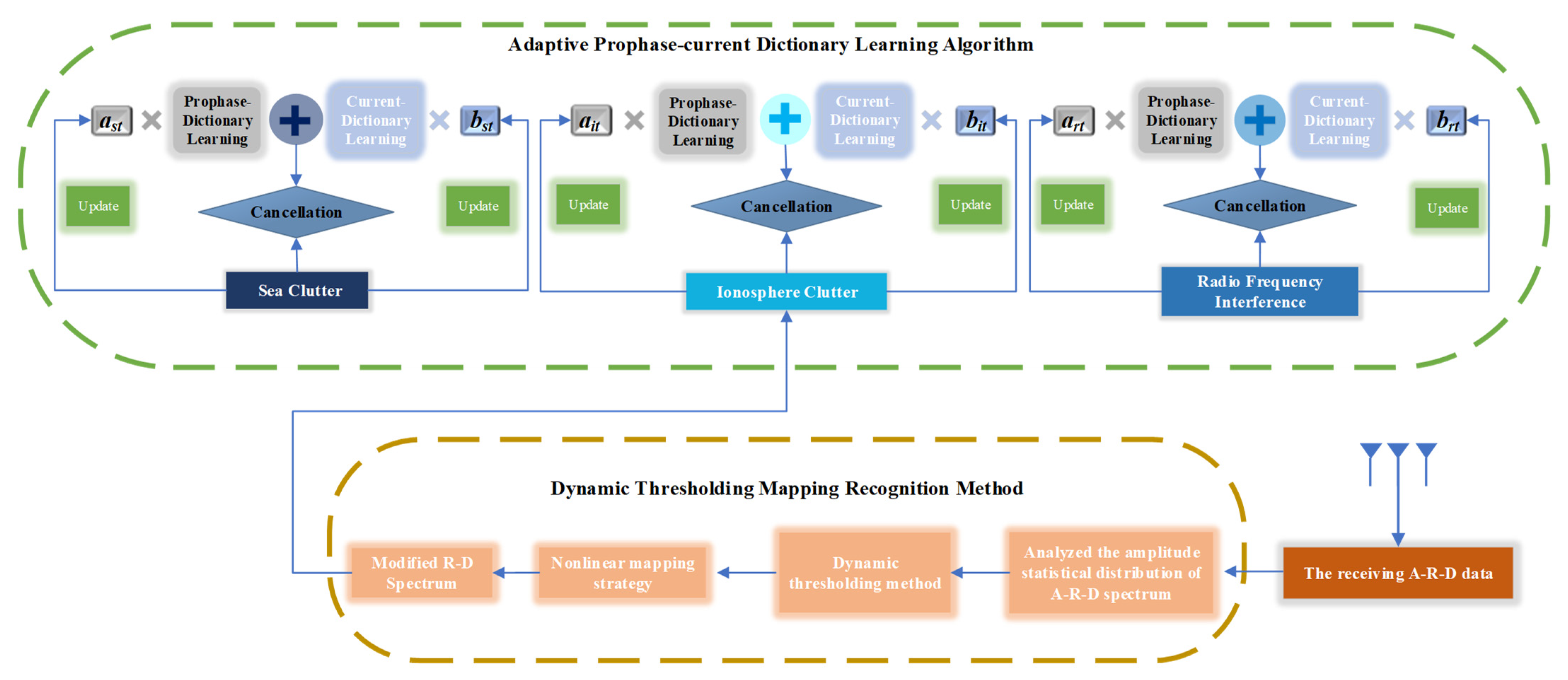
Clutter is non-Gaussian, non-linear and non-stationary, so empirically selecting a fixed dictionary is inappropriate for ever-changing clutter data. It can be predicted that the fixed dictionary has a lower matching degree with the current sea clutter, which cannot effectively remove sea clutter. For solving this problem, the first procedure of SMSF is using the recognition method (DTMR) to collect each type of learning data. The second procedure associatively mines the prophase and current characteristic information for eliminating all types of unwanted echo components and discovers the targets covered by clutter. The two procedures involve the development of a logical and repeatable methodology and we respectively introduce each part of the proposed framework. The operational flow diagram of the proposed framework is shown in Figure 4.
2.5.1. The First Step: Dynamic Threshold Mapping Recognition Method
Many proposed investigations for suppressing the sea or ionosphere clutter obtain the clutter characteristics based on RD images. The radar echo of a moving target occupies a small area on both the range and Doppler dimension. Sea clutter is distributed in the range domain and is confined to a narrow Doppler range. Ionosphere clutter as the trickiest clutter exhibits different behaviors or characteristics in the range-Doppler domain. Most ionosphere clutter suppression methods exploring characteristics in multiple domains are only applicable to one kind of ionosphere clutter, E or F layer.
The range-Doppler spectrum can collect the Doppler spectra of echo signals from each range bin and be plotted in a 3-D format. It can be shown as a pseudo-color image by mapping the amplitude information into different color channels. Traditionally, the color map scheme is Jet; it first normalizes the amplitude information of signals and then maps the normalized values into a color map. The qualitative color schemes have very limited choice when visualizing qualitative data, and the background noise of RD images in HFSWR is generally regarded as complex Gaussian noise. After a long period of observation and analysis, we find that the energy level of background noise is not always lower than that of the target pixels. The energy of background noise may increase at sunset. It is theorized that target signals and clutter will be confused by the noise with higher intensity, which greatly impacts the sequent detection and recognition. Hence, we first designed a nonlinear mapping preprocessing based on RD spectrum for the emergence of the targets and clutter with low SNR. We randomly select the pixels at often contaminated regions and then rank the magnitude value of selected pixels in an ascending sequence. We regard the median of this sequence as the threshold value; the threshold value selection can be written as
where represents the largest magnitude value of selected pixels, h means the number of selected pixels, is the threshold. The color of the RD image consists of three channel values. The magnitude of a pixel in an RD image can be expressed as . The represents the magnitude of the pixel located at coordinate for an RD image. P represents the number of Doppler cells in a received RD image. Q represents the number of range cells in a received RD image. We define the entire value of the three color channels of the pixel located at as . The value of each channel is obtained by the following equations.
Atmospheric noise, targets and unwanted echoes in different pixels with different magnitudes are distributed in an RD image. Prior information (signal-to-noise ratio rough range of each kind of echo component) and the characteristics of real-time data are useful guidelines for defining the range. The atmospheric noise is mapped into blue. The targets with low SNR (0–10 dB) are marked as indigo blue, which will be noticeable on the blue background. Next, the targets with medium SNR (10–20 dB) and the targets with high SNR (20–30 dB) are marked as green and yellow, respectively. The SNR of extremely strong echoes (mainly clutter and interference) is usually larger than 30 dB; these echo components are marked as red. The RD images mapped by the dynamic threshold are fed into the deep learning network for separating unwanted echo components.
In this experiment, we apply these collecting data and select sea clutter, banded ionosphere clutter, spread region ionosphere clutter and RFI as suppressed elements. The data mapped by the dynamic threshold are fed into the recognized network; in this experiment, the size of the entered RD images is and 50 RD images are selected as the training set. The training images are resized according to the design of the network and the epoch of the training network is 200. The task and process of DTMR are achieved. Of course, the selection of the deep learning network is various, the dynamic threshold mapping preprocessing is suitable for most networks, so we choose the YOLO algorithm in this experiment and obtain the ideal data set.
The classification results of the DTMR algorithm are listed in Table 1; we can see that the user’s accuracy for all kinds of classified data is more than 90%. These satisfying results indicate that each kind of selected component can be precisely sorted out and then formed into a different data set for subsequent learning. Results also prove that DTMR can reduce the image contamination caused by atmospheric noise and provide an RD image with cleaner background for recognizing the specific types of clutter.
2.5.2. The Second Step: Adaptive Prophase-Current Dictionary Learning Algorithm
In 24–25 August 2021, we observed the different types of clutter at a more than 16 h interval and noticed that the clutter exhibits variational behaviors as the time goes by. The clutter including sea clutter and ionosphere clutter is influenced by the external factors, so designing an adaptive and updated dictionary to precisely mine the characteristic of clutter is necessary for efficiently suppressing the clutter. To achieve this idea, we designed an Adaptive Prophase-current Dictionary Learning (APDL) algorithm. The rationale for this designation will be discussed in detail in the following steps.
Firstly, in order to explore the most optimal learning data for the dictionary, we designed two data screening schemes that are specific to the practical issue based on the K-svd algorithm. The first data screening scheme randomly selects the data in a long duration for the learning characteristic information and is named as Prophase-Dictionary Learning (PDL). In the PDL, in order to find the most suitable dictionary to represent the latest clutter data, the first step is setting the dictionary matrix with normalized columns. We randomly select five patches of data to train the prophase dictionary. The second step is the sparse coding stage; we take the sea clutter prophase dictionary obtained at t point as an example and donate it as . In this stage, the is fixed and the penalty term can be rewritten as:
where is the received sea clutter at t point and , is decoupled results for . is the sparse representation coefficients matrix of the sea clutter at t point and , is decoupled results for , and Hence, looking for the minimum of Equation (10) will obtain an optimal and this problem can be expressed as:
.
The problem is adequately addressed by pursuit algorithms. The third stage is updating the dictionary; each column in the dictionary is updated. The penalty term can be rewritten as:
where is one column of dictionary , and the coefficient that corresponds to it is , the row in . represents the error for N examples when the atom is removed. Then, the SVD is used to find alternative and .
The second data screening scheme only selects the latest clutter data to learn characteristic information and then these collecting data are fed into the dictionary; thus, it is called Current-Dictionary Learning (CDL). CDL only considers the latest clutter data and its building dictionary process is similar to the PDL.
In the APDL algorithm, we designed a hybrid selection mode; it randomly selects several patches of previous data and synchronously selects the latest data as the learning data set. Predictably, the hybrid selection mode mines the key information in all stages. We merge this hybrid selection mode with the APDL algorithm. Specifically, we donate the weight coefficient of PDL for sea clutter data at t point as and the weight coefficient of CDL for sea clutter at t point data as . Similarly, the weight coefficients of PDL and CDL for ionosphere clutter data at t point are donated as and , respectively. It needs to be emphasized that the types of received ionosphere clutter are unpredictable; thus, we classify the dramatically varying ionosphere clutter into two categories according to shape. The weight coefficients of PDL and CDL for banded ionosphere clutter are donated as and , respectively. The weight coefficients of PDL and CDL for spread region ionosphere clutter are donated as and , respectively. The weight coefficients of PDL and CDL for RFI data at t point are donated as and , respectively. The weight coefficients of each kind of undesired echo satisfy the following relationships.
Hence, finding the optimal weight coefficients at a specific moment is vital. Taking sea clutter learning as an example, finding optimal weight coefficients of two dictionary learning examples can be expressed as:
where the is the original sea clutter data at t point, is the learned sea clutter information by PDL, is the learned sea clutter information by CDL. Then, the atoms in are arranged in ascending order of values and these ranked atoms are donated as . The smaller atoms (top 80%) are added together; certainly, the sum of smaller atoms in means the sparse matrix and designed dictionary can exactly describe the estimated clutter . The top 80% atoms are used as a general rule of thumb, which is derived from a series of experiments.
The success of APDL is in the timely adjusting of each weight coefficient after the cancellation between learned clutter and real clutter. Consequently, the APDL algorithm can always describe the component to be estimated with the best sparse representations in a dynamic process. The characteristics of sea clutter change slowly when we observe the collected data set in Figure 5. Conversely, the behaviors of ionosphere clutter change rapidly and dramatically in a short period of time. The RFI does not have stationary rule in the time dimension, because it belongs to human interference. RFI may persist for a few hours, and persist for some minutes. The impetus for studying the time characteristics of different clutter and RFI is from the desire to obtain the moderate patches of learning data. The moderate quantity of learning data displays the accurate short-term trends of unwanted signals and decreases the computational cost. The moderate quantity of different types of clutter is diverse, but SMSF is a multi-mode suppression framework; the moderate quantity of learning data is set as a uniform parameter at each iteration. Algorithm 1 gives a detailed description of these steps.
| Algorithm 1 SMSF Framework |
| Procedure I: Input: A large amount of original echo data. Output: Each type of unwanted component data set: , , , .
Input: Learning data set: , , , . Output: The learned dictionary of each type of unwanted echo component obtained in Prophase Dictionary Learning at p point: , , , Initialization: Set all the dictionary matrix with normalized columns. Set the iterations of the dictionary learning J. Select batches of classified data set without overlapping and interference as learning data. Donate as , , , , respectively. While Train dictionary , , , in parallel.
Input: The echo data received from HFSWR at period is donated as . A patch of echo data received from HFSWR at point is donated as . Output: The processed RD image at point.
|
3. Results
3.1. Data Set
In this article, real data sets are generated from a small aperture HFSWR system with the specifications described in Table 2. Ionosphere clutter is the process resulting from the interaction between the ionosphere and the radar signal. Consequently, the observed behavior of the clutter relies on radar system parameters such as frequency, polarization, Pulse Repetition Frequency (PRF) and employed waveform. In the PDL process, the learning data set contains 1000 batches of receiving data and the data collection stretches over an extended period of time (over twenty hours). In the CDL processing, the learning data set contains several batches of data and the data collection stretches over a short time interval (several minutes). There are about 40,200 pixels in an RD image, which usually contains sea clutter, ground clutter, ionosphere clutter, radio frequency interference and targets.
3.2. Experimental Setup
The two classical clutter suppression methods are used to verify the effectiveness of the proposed SMSF; they are JDL and GSC. In the JDL, the size of the selected unit is ; 3 is the number of angular cells, 4 is the number of Doppler cells. In the GSC, the number of sub-array elements is 6.
For training the DTMR method, we apply 50 patches of collecting data as the training data set. In the dictionary learning processing, both the standardized width and height of the detection clutter region or RFI region determine the size of the dictionary. Obviously, different types of clutter have a different distribution area. In the sea clutter, the standardized size of the learning area is set as ; represents the number of Doppler cells contaminated by sea clutter at t point. The number of range cells of a whole RD image is 200 in most cases. As for RFI, the standardized size of the learning area is ; represents the number of Doppler cells contaminated by RFI at t point. In the ionosphere clutter, setting the standardized size becomes a troublesome problem because the ionosphere clutter may dramatically vary over several minutes. We set the standardized size of learning area as in a short period of time. The number of Doppler cells of a whole RD image is 201 in most cases. represents the number of range cells occupied by ionosphere clutter.
3.3. Novel Evaluation Indicators
It should be noted that the initial purpose of clutter suppression was observing specific target signals. However, many clutter suppression methods eliminate all types of radar echo components in the contaminated regions and target echoes are also removed, which is ineffective for realizing the initial purpose. The empirical measurements of previous methods are not suitable for our research. Therefore, we propose three novel evaluation indicators: Obscured Targets Detection Rate (OTDR), Clutter Purification Rate (CPR) and Erroneous Suppression Rate (ESR).
These evaluation indicators can be defined by referring to original RD images. Suppose the recognized clutter region is and the number of contaminated pixels in this area is . Assume that the number of remaining contaminated pixels is ; after using suppression methods, we can define CPR in region as:
.
We suppose that represents the number of obscured targets with a priori information in region , and represents the number of obscured targets found by using suppression methods. The can be expressed as:
.
The can be expressed as . These parameters evaluate the performance of each clutter suppression method in a more rational analysis, which facilitates the development of effective suppression algorithms.
3.4. The Suppression Results of Ionosphere Clutter
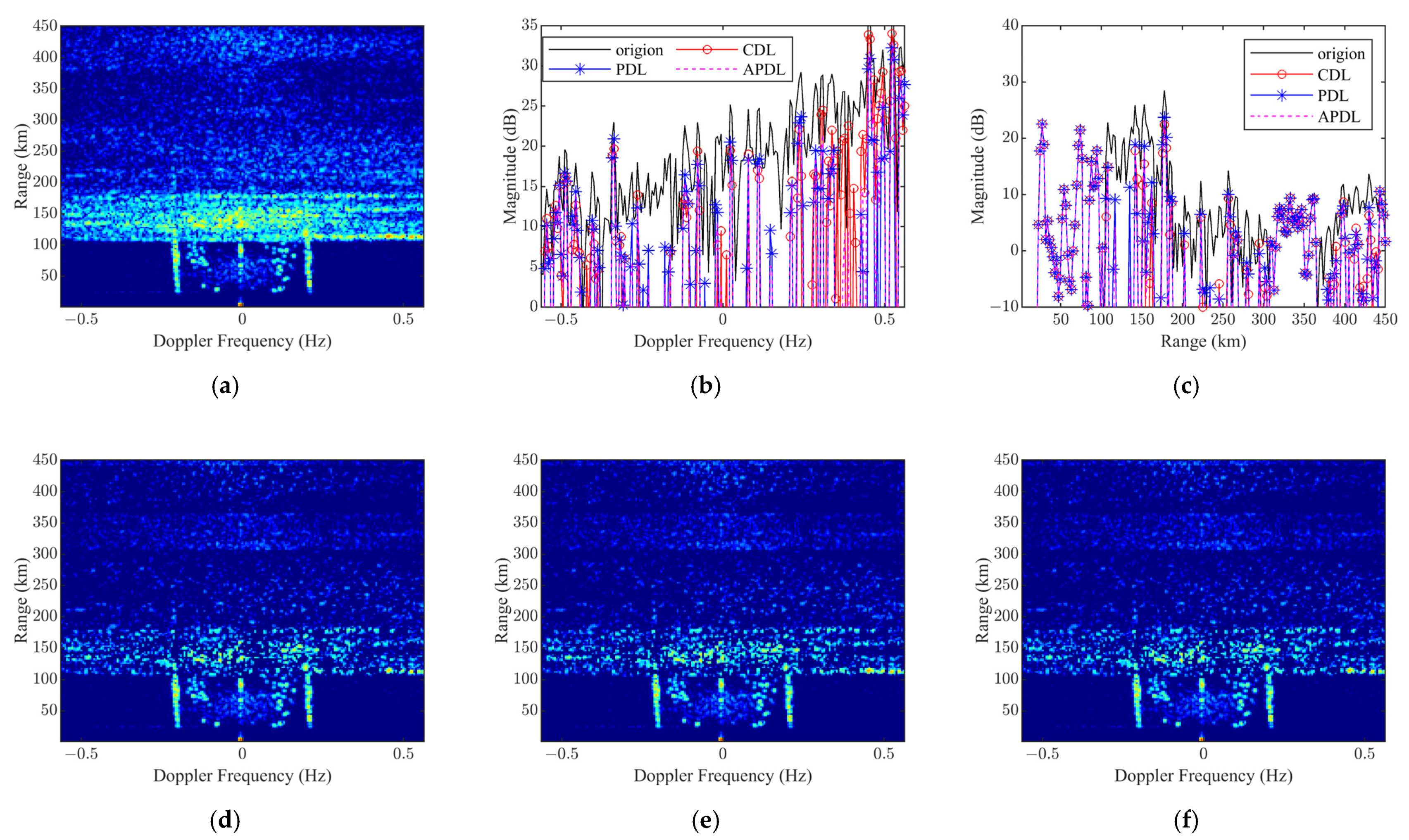
The suppression of polytropic ionosphere has many potential problems because of its hierarchical structure and various shapes. In the actual experiment, the first step aims at identifying the various shapes of ionospheric clutter, banded ionosphere clutter or spread region ionosphere clutter. Considering the shapes of ionosphere clutter, the suppression performance of related approaches will be separately compared. The banded ionosphere clutter is always from E-layer. The nominal height of the E-layer is 100 km and can range from 90 km to 140 km; it may cover the vessel targets. Fortunately, the E-layer usually occupies few range cells, thus it does not cover too many vessel targets. To allow a visual inspection, the suppressed RD images when applying different methods are displayed in Figure 5. Figure 5d,f suppress more clutter pollution than Figure 5e, which means that PDL and APDL can estimate the current ionosphere clutter in a sparse representation way. A more interesting factor is that CDL obtains unideal results by using several of the latest patches of echo data. The primary reason for this phenomenon is that the ionosphere clutter is rapidly changing, and the contiguous patches of data are diverse. Moreover, we can see that APDL always has more satisfying results than PDL and CDL from Figure 5b. In the right of Figure 5b, the performance of PDL is worse than that of CDL; the APDL still maintains superior estimation results.
The spread region ionosphere clutter always backscatters from the F-region. At night, the backscattered signal from the F-region occupies a much larger extent in both range and Doppler domains; many targets may be obscured into clutter. With respect to the performance comparison, we select the ionosphere clutter when it behaves in a most destructive way for detecting the target. In Figure 6b,c, both range profile and Doppler profile are used to verify the effectiveness of the proposed framework. The estimation performance of CDL is not stable; CDL obtains the optimal results when the Doppler frequency is more than 0.5 Hz, but it also has the worst results when the Doppler frequency is around 0 Hz. In Figure 6c, with the updating of dictionary learning, the learning accuracy of SMSF and PDL is consistently high. The efficiency of SMSF can be attributed to the fact that APDL can learn the potential dynamic rule in a long duration and mine the most representative information in the current, adaptively adjusting the learning emphasis between two phases.
3.5. The Suppression Results of Sea Clutter
The experimental results obtained with the compared algorithms and SMSF are presented in Figure 7. The general comments regarding the results are summarized as follows: First, the APDL achieves a more desired suppression performance than the PDL algorithm and CDL algorithm as visually shown in Figure 7d–f. This phenomenon can confirm that APDL has adaptive ability for the dynamic sea state. APDL takes both prophase data and current data into account, and the learning weights of two stages are adjusted according to the latest cancellation results. Timely capturing of the most representative information not only contributes to estimating clutter but also avoids removing the detected targets. We can also see that PDL has worse estimation results than the other two approaches in Figure 7c. This is a surprising result and also illustrates that sea clutter is not basically unchanged over an extended period. The commendable estimation results of CDL are enough to prove that the sea clutter is similar between current echoes and contiguous echoes. The second comment has approved this ability; we can find that the SMSF framework has the ability to reserve more simulated targets and realistic objectives. We will analyze this desired performance in the following experiment.
3.6. The Suppression Results of RFI
The RFI suppression is easier than clutter; the RD images of RFI suppression obtained with the different methods are displayed in Figure 8. SMSF and PDL achieve the ideal suppression performance in the non-edge and edge region. In the Doppler profile and range profile, the suppression effect of SMSF and PDL is always better than CDL, which means that their performance is fairly stable.
4. Discussion
The SMSF framework makes adjustments on the frequency of morphological variation of the ionosphere clutter and sea clutter. We evaluate the effectiveness of the proposed framework by conducting exhaustive experimental studies in multi-field applications. Different from the state-of-the-art methods that only pursue suppression effect, we consider the sustainable detection performance associated with clutter or interference, visual classification domains, suppression level of clutter and more importantly, the ability to expose targets covered by clutter. Finding the obscured vessels and concurrently removing the interference and clutter is a difficult task. The SMSF framework can admirably achieve this challenge and this ability has been approved in the following experiments.
4.1. Analysis of the Proposed SMSF Framework Based on Novel Evaluation Indicators
The initial goal of exploring clutter suppression methods was to offer continuous target surveillance and track surface vessels in a wide maritime environment. Hence, the proposed evaluation parameters can demonstrate the performance of SMSF in many views. CPR can assess the suppression effect of the algorithm; OTDR can assess the ability to excavate targets of the clutter suppression algorithm. Hence, we add ten simulated targets with different magnitudes into the real sea clutter data to assess the capability of finding the obscured targets and the correct purification capability. This process is shown in Figure 9.
For infinitely approaching the field experiment, the SNR is constantly adjusted with the magnitude of targets. Then, we apply the SMSF, JDL and GSC methods to suppress the clutter, respectively. Table 3 shows the OTDR results of the SMSF framework; the targets being colored grayish blue means that it cannot be found.
In accordance with Table 3, we draw the OTDR result curves of different algorithms, which clearly compare the difference in finding obscured target capability between SMSF and compared methods. We can also observe from Figure 10, in general, that the OTDR is decreasing, with the SNR and magnitude of simulated targets decreasing. When the simulated targets’ magnitude and SNR are relatively large (5/22.23 dB), SMSF expectedly uncovers the covered targets. Initially, when the SNR is low, the performance of JDL and GSC is better than SMSF. The OTDR of JDL is fluctuant, with the SNR increasing, but the overall trend is increasing. The GSC has the best detection performance in the initial stage, but the detection performance is abruptly destroyed with the SNR increasing. This phenomenon can be attributed to the fact that the rising target amplitude and SNR cause the target energy to be leaked into the sidelobe; thereby, the auxiliary beam will mistakenly regard the echo signal as clutter and suppress this “clutter”; actually, they are targets with strong power. Hence, the value of OTDR drops suddenly. With the SNR increasing, the detection performance of SMSF is constantly being enhanced and SMSF achieves the perfect detection results when the SNR exceeds 0 dB.
4.2. Motion Tracking Experiment of Proposed SMSF
We have recognized that the adaptive capacity of clutter suppression is very significant for varying data; thus, we select several continuous batches of echo data received by HFSWR, which are utilized to confirm that SMSF can suppress the clutter and synchronously preserve real targets. We found that a target was emerging from the sea clutter, thus we select several continuous batches of echo data. As shown in Figure 11, this travelling target is escaping from the sea clutter in five CIT intervals. The serial pictures in the second row represent the RD images suppressed by SMSF, and the red circle marks the travelling target. We can observe that this travelling target persists over the entire observation period (7 min). This experiment result also indicates that SMSF can maintain ideal suppression performance in changing scenarios, and the travelling targets can be continuously observed.
4.3. Suppression Performance Comparison in Doppler Domain
The adaptive capacity of clutter suppression is very significant for varying data, so we also chose a batch of echo data for comparing the suppression performance in the Doppler domain between SMSF and other compared methods. In Figure 12, SMSF can effectively suppress sea clutter while retaining the target merged into the sea clutter. This can be attributed to the fact that SMSF can accurately learn the underlying characteristics of sea clutter, and can avoid mistakenly eliminating the target signal. JDL and GSC methods can also suppress the sea clutter without targets as shown in the left of Figure 12. However, these compared methods weaken the magnitude of targets, especially JDL, which violates the original purpose of clutter suppression methods and has a negative effect on the subsequent target detection. After using the JDL method, we just obtain a clean RD image, which does not include the covered targets.
4.4. Technical Innovations of SMSF
All the experiment results have confirmed that SMSF has the expected suppression performance and finding target ability, which is attributed to the technical innovations of SMSF. The foremost innovations are strong adaptability of SMSF for varying echo data, and the self-regulating ability of SMSF in real-time processing. SMSF can express the unwanted echoes in sparse representation by adequately learning historical data to find their similarities. SMSF learns the current data in good time for capturing the latest information. Under this design, SMSF reduces the sensitivity of data selection and also decreases the dependence on the training set, of which the second is an innovation. According to the latest received clutter data as a reference, the information learned by historical data and the current data is optimized in real time; the balance between the two different learning stages is adjusted to fit the latest received clutter data, thus the optimal representation can be found. SMSF is a remedy to solve the problem of JDL, but the final suppression results are not limited to training sample selection. The third innovation of SMSF is its wide applicability; SMSF can suppress many types of clutter and RFI. By incorporating the deep learning network, every type of clutter is sorted out for dictionary learning. This design circumvents a perennial obstacle insofar as each type of clutter is suppressed by each specific method. However, SMSF does not use spatial information to its full potential, and the suppression performance is not ideal when the Signal Clutter Ratio (SCR) is low, so the dimension of dictionary learning will be further increased in the future work.
5. Conclusions
For accommodating varying clutter and arbitrary RFI, this paper introduces SMSF with dynamically updating performance and adaptive learning ability to suppress unwanted echo components. The multidimensional characteristics of each type of undesired echo component are various. Therefore, in order to observe the behaviors of each type of unwanted reception signal precisely, we first propose a novel denoising method (DTMR) for suppressing the background noise in a general RD image. Then, SMSF applies a superior deep learning algorithm to recognize each type of unwanted reception signal and divides them into different categories. Each set of classified data contains a type of unwanted reception signal. Next, these classified data are fed into the novel dictionary learning algorithm (APDL). APDL algorithm captures the underlying information for each type of unwanted reflection signal based on the current classified data set and the prophase classified data set. As an adaptive process, the APDL self-regulates the weights of learning data sets in different phases to better fit the real clutter echo signal and also automatically refresh dictionary atoms.
The echo data received from the actual HFSWR system in Weihai have verified the effectiveness of the proposed SMSF. SMSF can suppress the unwanted reflection signal component from the composite radar returns and uncover targets obscured by clutter or interference. Encouragingly, SMSF can constantly recognize the travelling track of a real target in several minutes. Finding out the obscured targets is an intractable issue such that many published papers do not achieve information on obscured targets, but SMSF expectedly realizes this challenge.
There is still much room for improvement in SMSF. In particular, there is a need to use Automatic Identification System (AIS) data to verify the positions of more obscured ships, such as those covered by the RFI and Es layer ionosphere, thereby assessing the performance of the proposed SMSF. Furthermore, it would be preferable to continuously track the vessel targets and depict the track with cooperating sequential received data. All the above mentioned experiments should be conducted in various times and weather, since local conditions markedly influence the effectiveness of the proposed scheme.
Author Contributions
Methodology, validation, writing—original draft preparation, X.J.; software, validation, L.W.; supervision, funding acquisition, Q.Y. All authors have read and agreed to the published version of the manuscript.
Funding
This work was supported in part by Hainan Province Key Research and Development Project under Grant ZDYF2019195, in part by the National Natural Science Foundation of China under Grant 62031014.
Data Availability Statement
Not applicable.
Conflicts of Interest
The authors declare no conflict of interest.
References
- Chan, H.C. Characterization of Ionospheric Clutter in HF Surface-Wave Radar; Technical Report TR 2003-114; Defence Research and Development Canada (DRDC): Ottawa, ON, Canada, 2003.
- Thayaparan, T.; Dupont, D.; Ibrahim, Y.; Riddolls, R. High-Frequency Ionospheric Monitoring System for Over-the-Horizon Radar in Canada. IEEE Trans. Geosci. Remote Sens. 2019, 57, 6372–6384. [Google Scholar] [CrossRef]
- Walsh, J.; Huang, W.; Gill, E.W. An analytical model for HF radar ionospheric clutter. In Proceedings of the 2013 IEEE Antennas and Propagation Society International Symposium (APSURSI), Orlando, FL, USA, 7–13 July 2013; pp. 1974–1975. [Google Scholar]
- Thayaparan, T.; MacDougall, J. Evaluation of ionospheric sporadic-E clutter in an arctic environment for the assessment of high-frequency surface-wave radar surveillance. IEEE Trans. Geosci. Remote Sens. 2005, 43, 1180–1188. [Google Scholar] [CrossRef]
- Yang, X.; Wang, M.; Huang, W.; Yu, C. Experimental Observation and Analysis of Ionosphere Echoes in the Mid-Latitude Region of China Using High-Frequency Surface Wave Radar and Ionosonde. IEEE J. Sel. Top. Appl. Earth Obs. Remote Sens. 2020, 13, 4599–4606. [Google Scholar] [CrossRef]
- Ravan, M.; Riddolls, R.J.; Adve, R.S. Ionospheric and auroral clutter models for HF surface wave and over the horizon radar systems. Radio Sci. 2012, 47, 1–12. [Google Scholar] [CrossRef]
- Chen, S.; Gill, E.W.; Huang, W. A First-Order HF Radar Cross-Section Model for Mixed-Path Ionosphere–Ocean Propagation with an FMCW Source. IEEE J. Ocean. Eng. 2016, 41, 982–992. [Google Scholar] [CrossRef]
- Chen, S.; Gill, E.W.; Huang, W. A High-Frequency Surface Wave Radar Ionospheric Clutter Model for Mixed-Path Propagation with the Second-Order Sea Scattering. IEEE Trans. Antennas Propag. 2016, 64, 5373–5381. [Google Scholar] [CrossRef]
- Aboutanios, E.; Mulgrew, B. Hybrid detection approach for STAP in heterogeneous clutter. IEEE Trans. Aerosp. Electron. Syst. 2010, 46, 1021–1033. [Google Scholar] [CrossRef]
- Zhou, Q.; Yue, X.; Zhang, L.; Wu, X.; Wang, L. Correction of ionospheric distortion on HF hybrid sky-surface wave radar calibrated by direct wave. Radio Sci. 2019, 54, 380–396. [Google Scholar] [CrossRef]
- Hua, X.; Ono, Y.; Peng, L.; Cheng, Y.; Wang, H. Target detection within nonhomogeneous clutter via total bregman divergence-based matrix information geometry detectors. IEEE Trans. Signal Process. 2021, 69, 4326–4340. [Google Scholar] [CrossRef]
- Barrick, D.E.; Headrick, J.M.; Bogle, R.W.; Crombie, D.D. Sea backscatter at HF: Interpretation and utilization of the echo. Proc. IEEE 1974, 62, 673–680. [Google Scholar] [CrossRef]
- Wang, Z.Q.; Li, Y.J.; Shi, J.N.; Wang, P.F.; Chen, D.H. Spread Sea Clutter Suppression in HF Hybrid Sky-Surface Wave Radars Based on General Parameterized Time-Frequency Analysis. Int. J. Antennas Propag. 2020, 3, 7627521. [Google Scholar] [CrossRef]
- Sevgi, L.; Ponsford, A.; Chan, H.C. An integrated maritime surveillance system based on high-frequency surface wave radars, part 1: Theoretical background and numerical simulations. IEEE Antennas Propag. Mag. 2001, 43, 28–42. [Google Scholar] [CrossRef]
- Zhao, L.; Sun, J.; Xu, X. A hybrid STAP approach to target detection for heterogeneous scenarios in radar seekers. Multidim. Syst. Sign. Process. 2014, 25, 493–509. [Google Scholar] [CrossRef]
- Li, G.Q.; Song, Z.Y.; Fu, Q. A convolutional neural network based approach to sea clutter suppression for small boat detection. Front. Inform. Technol. Electron. Eng. 2020, 21, 1504–1520. [Google Scholar] [CrossRef]
- Doulamis, A.D.; Shang, S.; He, K.N.; Wang, Z.B.; Yang, T.; Liu, M.; Li, X. Sea Clutter Suppression Method of HFSWR Based on RBF Neural Network Model Optimized by Improved GWO Algorithm. Comput. Intell. Neurosci. 2020, 2020, 8842390. [Google Scholar] [CrossRef]
- Zhang, L.; You, W.; Wu, Q.; Qi, S.; Ji, Y. Deep Learning-Based Automatic Clutter/Interference Detection for HFSWR. Remote Sens. 2018, 10, 1517. [Google Scholar] [CrossRef] [Green Version]
- Chen, Z.; Xie, F.; Zhao, C.; He, C. Radio frequency interference mitigation for high-frequency surface wave radar. IEEE Geosci. Remote Sens. Lett. 2018, 15, 986–990. [Google Scholar] [CrossRef]
- Yao, D.; Deng, W.B.; Zhang, X.; Yang, Q.; Zhang, J.Z.; Li, J.M. Main-lobe clutter suppression algorithm based on rotating beam method and optimal sample selection for small-aperture HFSWR. IET Radar Sonar Navig. 2019, 13, 1162–1170. [Google Scholar] [CrossRef]
- Liu, Z.; Su, H.; Hu, Q. Radio Frequency Interference Cancelation for Skywave Over-the-Horizon Radar. IEEE Geosci. Remote Sens. Lett. 2016, 13, 304–308. [Google Scholar] [CrossRef]
- Wang, W.; Wyatt, L.R. Radio frequency interference cancellation for sea-state remote sensing by high-frequency radar. IET Radar Sonar Navig. 2011, 5, 405–415. [Google Scholar] [CrossRef]
- Li, Y.H.; Yue, X.C.; Wu, X.B.; Zhang, L.; Zhou, Q.; Yi, X.Z.; Liu, N. A Higher-Order Singular Value Decomposition-Based Radio Frequency Interference Mitigation Method on High-Frequency Surface Wave Radar. IEEE Trans. Geosci. Remote Sens. 2020, 58, 2770–2781. [Google Scholar] [CrossRef]
- Eslami Nazari, M.; Huang, W.; Zhao, C. Radio Frequency Interference Suppression for HF Surface Wave Radar Using CEMD and Temporal Windowing Methods. IEEE Geosci. Remote Sens. Lett. 2020, 17, 212–216. [Google Scholar] [CrossRef]
- Zhou, H.; Wen, B. Radio frequency interference suppression in small-aperture high-frequency radars. IEEE Geosci. Remote Sens. Lett. 2012, 9, 788–792. [Google Scholar] [CrossRef]
- Hua, X.; Peng, L. MIG Median Detectors with Manifold Filter. Signal Processing 2021, 188, 108176. [Google Scholar] [CrossRef]
- Zhang, L.; Li, Q.F.; Wu, Q.J. Target Detection for HFSWR Based on an S3D Algorithm. IEEE Access 2020, 8, 224825–224836. [Google Scholar] [CrossRef]
- Aziz, L.; Haji Salam, M.S.B.; Sheikh, U.U.; Ayub, S. Exploring Deep Learning-Based Architecture, Strategies, Applications and Current Trends in Generic Object Detection: A Comprehensive Review. IEEE Access 2020, 8, 170461–170495. [Google Scholar] [CrossRef]
- Girshick, R. Fast R-CNN. In Proceedings of the 2015 IEEE International Conference on Computer Vision (ICCV), Santiago, Chile, 7–13 December 2015; pp. 1440–1448. [Google Scholar]
- Azhagu Jaisudhan Pazhani, A.; Vasanthanayaki, C. Object detection in satellite images by faster R-CNN incorporated with enhanced ROI pooling (FrRNet-ERoI) framework. ESIN 2022, 15, 553–561. [Google Scholar]
- Wu, W.; Liu, H.; Li, L.; Long, Y.; Wang, X.; Wang, Z.; Li, J.; Chang, Y. Application of local fully Convolutional Neural Network combined with YOLO v5 algorithm in small target detection of remote sensing image. PLoS ONE 2021, 16, e0259283. [Google Scholar] [CrossRef]
- Liu, D.Y.; Liang, C.W.; Chen, S.K.; Tie, Y.; Qi, L. Auto-encoder based structured dictionary learning for visual classification. Neurocomputing 2021, 438, 34–43. [Google Scholar] [CrossRef]
- Wang, Z.; Shi, S.; He, Z.; Sun, G.; Cao, J. An ocean clutter suppression method for OTHR by combining optimal filter and dictionary learning. In Proceedings of the 2018 IEEE Radar Conference (RadarConf18), Oklahoma City, OK, USA, 23–27 April 2018; pp. 1499–1503. [Google Scholar]
- Rosenberg, L.; Duk, V.; Ng, B. Practical detection using sparse signal separation. In Proceedings of the International Radar Conference, Florence, Italy, 21–25 September 2020. [Google Scholar]
- Aharon, M.; Elad, M.; Bruckstein, A. K-SVD: An algorithm for designing overcomplete dictionaries for sparse representation. IEEE Trans. Signal Process. 2006, 54, 4311–4322. [Google Scholar] [CrossRef]
- Zhang, X.; Deng, W.; Yang, Q.; Dong, Y. Modified Space-Time Adaptive Processing with first-order bragg lines kept in HFSWR. In Proceedings of the 2014 International Radar Conference, Lille, France, 13–17 October 2014; pp. 1–4. [Google Scholar]
- Buckley, K.; Griffiths, L. An adaptive generalized sidelobe canceller with derivative constraints. IEEE Trans. Antennas Propag. 1986, 34, 311–319. [Google Scholar] [CrossRef]
- Zhang, X.; Yao, D.; Yang, Q.; Dong, Y.N.; Deng, W.B. Knowledge-Based Generalized Side-Lobe Canceller for Ionospheric Clutter Suppression in HFSWR. Remote Sens. 2018, 10, 104. [Google Scholar] [CrossRef] [Green Version]
Figure 1.
Real scenario of coexistence of vessel targets, background noise, ionosphere clutter, sea clutter and ground clutter in an HFSWR RD image.
Figure 1.
Real scenario of coexistence of vessel targets, background noise, ionosphere clutter, sea clutter and ground clutter in an HFSWR RD image.

Figure 2.
Localized processing region in the JDL.

Figure 3.
The framework of the GSC.

Figure 4.
Operational flow diagram of SMSF framework.

Figure 5.
The suppression results of banded ionosphere clutter from using different dictionary learning algorithms. (a) Original RD images; (b) the Doppler profile of banded ionosphere clutter suppressed by SMSF; (c) the range profile of banded ionosphere clutter suppressed by SMSF; (d) the suppression results of PDL algorithm; (e) the suppression results of CDL algorithm; (f) the suppression results of SMSF framework.

Figure 6.
The suppression results of spread region ionosphere clutter from using different dictionary learning algorithms. (a) Original RD images; (b) the Doppler profile of spread region ionosphere clutter suppressed by SMSF; (c) the range profile of spread region ionosphere clutter suppressed by SMSF; (d) the suppression results of PDL algorithm; (e) the suppression results of CDL algorithm; (f) the suppression results of SMSF.

Figure 7.
The suppression results of sea clutter from using different dictionary learning algorithms. (a) Original RD images; (b) the Doppler profile of sea clutter suppressed by SMSF; (c) the range profile of sea clutter suppressed by SMSF; (d) the suppression results of PDL algorithm; (e) the suppression results of CDL algorithm; (f) the suppression results of SMSF.

Figure 8.
The suppression results of RFI from using different dictionary learning algorithms. (a) Original RD images; (b) the Doppler profile of RFI suppressed by SMSF; (c) the range profile of RFI suppressed by SMSF; (d) the suppression results of PDL algorithm; (e) the suppression results of CDL algorithm; (f) the suppression results of SMSF.


Figure 9.
The experiment process of the SMSF performance assessment using novel evaluation indicators.
Figure 9.
The experiment process of the SMSF performance assessment using novel evaluation indicators.

Figure 10.
The comparison of OTDR between SMSF and compared methods.

Figure 11.
The dynamic suppression results of sea clutter using SMSF in five sequential CITs.

Figure 12.
The Doppler profiles of clutter suppression results using different suppression methods.


Table 1.
Classification accuracies obtained by DTMR algorithm.
| Classified Data | Reference Data | ||||||
|---|---|---|---|---|---|---|---|
| Sea Clutter | Banded Ionosphere Clutter | RFI | Ground Clutter | Spread Region Ionosphere Clutter | Total | UA (%) | |
| Sea Clutter | 96 | 0 | 0 | 0 | 0 | 96 | 100% |
| Banded Ionosphere Clutter | 1 | 151 | 0 | 0 | 1 | 153 | 99% |
| RFI | 0 | 0 | 6 | 0 | 0 | 6 | 100% |
| Ground Clutter | 1 | 0 | 0 | 45 | 0 | 46 | 98% |
| Spread Region Ionosphere Clutter | 0 | 6 | 0 | 0 | 69 | 75 | 92% |
| Background | 1 | 30 | 2 | 3 | 9 | 45 | |
| Total | 99 | 187 | 8 | 48 | 79 | ||
| PA (%) | 97% | 81% | 75% | 94% | 87% | ||
UA = user’s accuracy, PA = producer’s accuracy.
Table 2.
The Operating Parameters of HFSWR.
| Properties | Specification |
|---|---|
| Frequency bandwidth | 60 kHz |
| Carrier frequency | 4.7 MHz |
| Coherent Integration Time | 144 s |
| Range cell | 200 |
| Doppler cell | 201 |
| Waveform | FMICW |
Table 3.
The OTDR of ten simulated targets using SMSF.
| The Serial Number of Simulated Targets | 1 | 2 | 3 | 4 | 5 | 6 | 7 | 8 | 9 | 10 | OTDR (%) | |
|---|---|---|---|---|---|---|---|---|---|---|---|---|
| SNR/The Magnitude of Simulated Targets (dB) | ||||||||||||
| The Magnitude of Simulated Target after Being Suppressed (dB) | ||||||||||||
| 20/38.81 (dB) | 34.82 | 19.78 | 24.06 | 27.63 | 22.50 | 29.17 | 26.59 | 26.75 | 24.44 | 16.12 | 100% | |
| 20/37.23 (dB) | 23.16 | 12.28 | 14.47 | 34.34 | 21.19 | 27.24 | 11.28 | 27.63 | 26.12 | 24.95 | 100% | |
| 15/33.82 (dB) | −12.12 | 6.92 | −19.78 | 6.57 | 12.55 | −16.64 | −4.54 | −13.60 | −0.53 | 24.20 | 90% | |
| 15/32.23 (dB) | 8.67 | 17.86 | 18.26 | 20.36 | 24.35 | 24.01 | 15.29 | 24.11 | 18.56 | 13.86 | 80% | |
| 10/28.82 (dB) | 1.28 | 18.12 | −7.07 | 8.44 | −14.06 | −10.97 | 17.15 | 10.20 | 8.14 | 1.28 | 70% | |
| 10/27.23 (dB) | 12.83 | 1.09 | 14.33 | 16.44 | 18.45 | 10.19 | −17.95 | 15.21 | 9.42 | 21.80 | 80% | |
| 5/23.82 (dB) | −2.13 | −6.38 | 13.56 | 8.32 | −8.73 | 8.45 | −14.25 | −4.11 | 6.77 | −7.68 | 70% | |
| 5/22.23 (dB) | 9.23 | 18.93 | 7.47 | −7.08 | 11.10 | 15.97 | 19.20 | −17.62 | 14.84 | 10.60 | 80% | |
| 0/18.82 (dB) | 2.84 | 5.30 | −9.11 | 2.34 | −2.59 | 8.92 | −8.55 | −4.65 | −15.87 | 16.41 | 60% | |
| 0/17.23 (dB) | 9.85 | 5.86 | −2.88 | 0.09 | −13.08 | −0.61 | 8.59 | 1.51 | 8.13 | −8.14 | 50% | |
| −5/13.83 (dB) | −3.19 | 4.63 | 15.05 | −7.81 | −8.58 | 5.86 | −16.87 | −22.44 | 0.89 | −1.62 | 60% | |
| −5/12.23 (dB) | −20.23 | 0.36 | −5.38 | −5.69 | −18.14 | −22.02 | −7.46 | −24.31 | −10.84 | 4.48 | 40% | |
| −10/8.82 (dB) | 3.01 | −16.38 | −9.11 | −11.39 | 2.48 | −0.37 | −3.01 | −5.15 | −3.91 | −6.71 | 40% | |
| −10/7.23 (dB) | 3.11 | −0.45 | −1.32 | −4.20 | −2.77 | 4.76 | 7.52 | −5.11 | −1.14 | −3.61 | 70% | |
| −15/3.82 (dB) | −8.89 | −15.42 | −9.72 | −1.69 | −8.59 | −15.03 | −16.45 | −4.88 | −14.39 | −13.64 | 30% | |
| −15/2.23 (dB) | −18.73 | −10.58 | −3.90 | −3.92 | −12.85 | −8.83 | −9.65 | −7.68 | −12.20 | −12.76 | 30% | |
| −20/−1.18 (dB) | −10.33 | −12.66 | −9.11 | −10.32 | −2.16 | −5.64 | −36.72 | −11.50 | −2.56 | −3.52 | 20% | |
| −20/−2.77 (dB) | −7.98 | 4.65 | −12.35 | −9.94 | −21.56 | −3.37 | −3.28 | −11.32 | −10.90 | −8.92 | 30% | |
Publisher’s Note: MDPI stays neutral with regard to jurisdictional claims in published maps and institutional affiliations. |
© 2022 by the authors. Licensee MDPI, Basel, Switzerland. This article is an open access article distributed under the terms and conditions of the Creative Commons Attribution (CC BY) license (https://creativecommons.org/licenses/by/4.0/).
Share and Cite
MDPI and ACS Style
Ji, X.; Yang, Q.; Wang, L. A Self-Regulating Multi-Clutter Suppression Framework for Small Aperture HFSWR Systems. Remote Sens. 2022, 14, 1901. https://0-doi-org.brum.beds.ac.uk/10.3390/rs14081901
AMA Style
Ji X, Yang Q, Wang L. A Self-Regulating Multi-Clutter Suppression Framework for Small Aperture HFSWR Systems. Remote Sensing. 2022; 14(8):1901. https://0-doi-org.brum.beds.ac.uk/10.3390/rs14081901
Chicago/Turabian StyleJi, Xiaowei, Qiang Yang, and Linwei Wang. 2022. "A Self-Regulating Multi-Clutter Suppression Framework for Small Aperture HFSWR Systems" Remote Sensing 14, no. 8: 1901. https://0-doi-org.brum.beds.ac.uk/10.3390/rs14081901
Note that from the first issue of 2016, this journal uses article numbers instead of page numbers. See further details here.