Low-SNR Doppler Data Processing for the InSight Radio Science Experiment

Abstract

Radio Doppler measurements between the InSight lander and NASA’s Deep Space Network have been acquired for measuring the rotation of Mars. Unlike previous landers used for this purpose that utilized steerable high-gain antennas, InSight uses two fixed medium-gain antennas, which results in a lower radio signal-to-noise ratio (SNR). Lower SNR results in additional thermal noise for Doppler measurements using standard processes. Through a combination of phase averaging and traditional data compression, the increased thermal noise due to low SNR can be removed for most of the signal of interest, resulting in more accurate Doppler measurements. During the first 900 days of InSight operations, Doppler measurements were improved by ~25% on average using this method.

1. Introduction

NASA’s Deep Space Network (DSN) is a set of ground stations that support the command, telemetry, and tracking of planetary probes. The measurement of the carrier frequency of the downlink signal, commonly referred to as the Doppler measurement, is used primarily for spacecraft navigation and the measurement of planetary gravity fields and rotation properties. In a majority of cases, Doppler measurements are made using a spacecraft’s high-gain antenna on the spacecraft pointed directly at Earth. Routine Doppler measurements are generated by the DSN’s closed-loop receiver using a phase-locked loop process, which runs in near real time. This phase-locked loop relies on a prediction of the expected spacecraft signal frequency [1].

In some applications, such as those with large uncertainty in signal amplitude or frequency (e.g., radio occultation, planetary flybys), the radio signal can be directly recorded by an open-loop receiver (OLR) which measures the down-converted antenna voltage. This signal can be post-processed with a tunable phase-locked loop or fast-Fourier transform analysis to produce a radio Doppler measurement where the closed-loop receiver may either not function or have increased thermal noise. This open-loop recording process is very flexible but often requires additional processing time and cost.

Doppler measurements of previous landers on Mars, specifically Viking Lander 1, Mars Pathfinder, and Mars Exploration Rovers [2], used steerable high-gain antennas, providing high strength signals to the DSN for tracking. InSight uses Doppler measurements to further constrain Mars rotation [3]. In order to reduce the cost of InSight, the lander instead utilizes two non-steerable medium-gain antennas (MGA), one east-facing and one west-facing, for Doppler measurements, uplink commanding, and low-rate communications. The lower signal-to-noise (SNR) ratio of the InSight Doppler measurements (~13–30 dB-Hz, versus a typical orbiter >40 dB-Hz) results in increased noise in the Doppler data when acquired with the closed-loop receiver. The additional noise can be removed for time scales longer than ~20 s using both phase-averaging and frequency-averaging techniques. This paper describes the standard DSN Doppler measurement process, summarizes the basic measurement noise types with details on the effect on low-SNR signals, and describes the processes used for InSight to show the improvement in Doppler measurement noise.

These processes may be useful for future missions planning to use medium-gain antennas or low-gain antennas for Doppler measurement, for example, the Lander Radio science experiment on ExoMars [4] and the gravity experiment for Europa Clipper [5].

2. DSN Doppler Measurement Process

DSN Doppler measurements are difference-phase measurements. The Doppler measurement f is the difference of the received radio signal phase ϕ at two times, separated by the time interval (called the count time, T_c), with a time tag halfway between the times of the two phase measurements [6]:

$$f\left(t\right)=-\frac{\varphi \left(t-\frac{T_c}{2}\right)-\varphi \left(t+\frac{T_c}{2}\right)}{T_c}$$

(1)

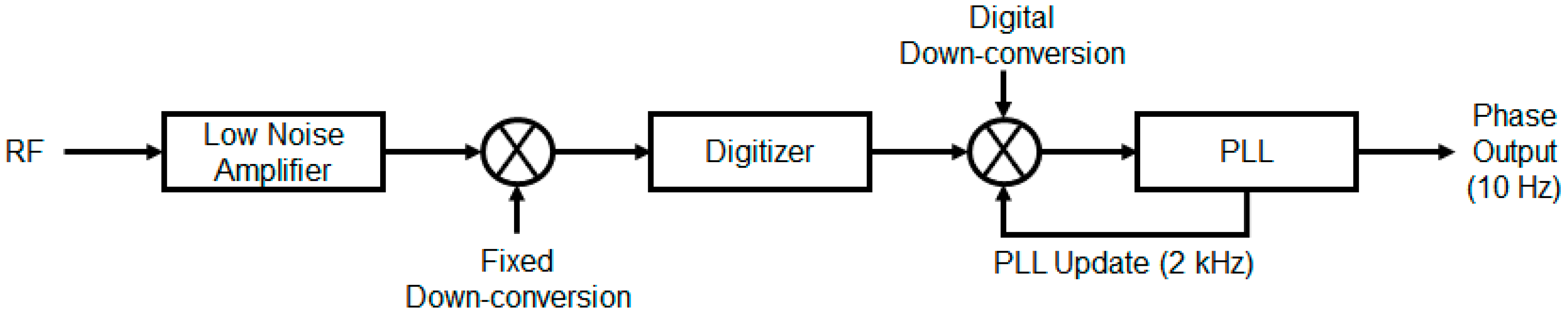
Since the mid-1990s, the Doppler measurements have been made by the Block V Receiver (BVR) [7] that is now part of the Downlink Tracking and Telemetry Subsystem (Module 202D of [1]). Figure 1 shows a simplified block diagram of the process; for more details, refer to [1,7].

The spacecraft radio signal is down-converted from radio frequency (RF) to an intermediate frequency (IF) of about 200 MHz using a fixed frequency downconverter. The IF signal is undersampled at 160 Msamples/sec to provide a band from 0 to 80 MHz. The spacecraft carrier is at about 40 MHz in this band. Quadrature down-conversion to baseband is then used to generate complex samples at a rate of 80 Msamples/sec with the spacecraft carrier near 0 MHz. All further processing is performed at this sample rate.

The digital samples are mixed with a phase model that is based on frequency predicts. The residual signal, spacecraft minus model, is processed using a digital phase-lock-loop (PLL) with a bandwidth B_L sufficiently wide to cover the likely prediction errors and other variations in the signal [8]. The PLL model is updated at a rate of 2 kHz (the update period is thus 0.5 milliseconds) using all data up to the current time. The updated model, along with the previous data within the filter time constant 1/(2B_L), is used for phase estimation for the next 0.5 milliseconds. Each sample has an effective integration time of 1/(2B_L). The phase output of the PLL is sampled by the BVR at the fixed rate of 0.1 s. Phase is recorded at the RF level. A user may request Doppler measurements with a count time of any integer multiple of 0.1 s. These Doppler observables are generated as in Equation (1), and for InSight, 0.1 s BVR phase samples are used at the end points of the requested count time interval with a loop bandwidth B_L of 5 Hz.

3. Doppler Measurement Noise

A majority of current planetary spacecraft tracked by the DSN use the deep-space X-band spectrum allocation (~7.2 GHz uplink from Earth to spacecraft, and ~8.4 GHz downlink from spacecraft to Earth). Doppler measurement noise for these links is usually dominated by fluctuations in water vapor in the Earth’s troposphere along the line of sight between the DSN antenna to the spacecraft. When the path of the radio signal is close to the sun, the Doppler noise can be dominated by fluctuations in density of electrons (solar plasma). Solar plasma noise on Doppler measurements is proportional to the inverse-square of the radio frequency, and therefore is larger for spacecraft that utilize S-band (2.1 GHz) and smaller for spacecraft that utilize Ka-band (32 GHz) [9].

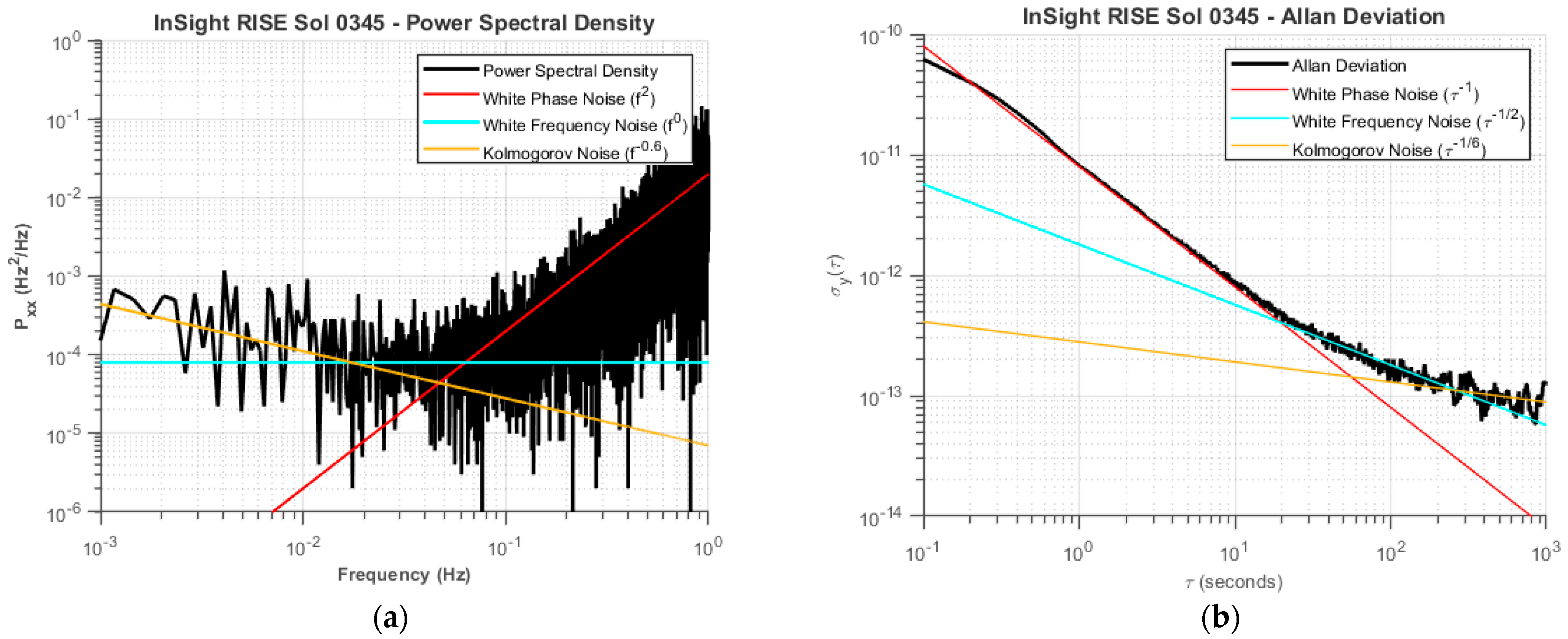
The source of the noise for a given Doppler track can be identified from its power spectrum or, equivalently, from the Allan deviation [10]. Thermal noise from finite SNR in the link behaves as white phase noise, with an Allan deviation slope of τ⁻¹ [11]. The noise due to water vapor fluctuations behaves as white frequency noise [12], and the noise due to solar plasma behaves as Kolmogorov noise [13]. The corresponding slopes in the Allan deviation are τ^−1/2 and τ^−1/6, respectively.

There are other sources of Doppler noise that are smaller than the troposphere noise that are usually negligible, including noise in the DSN time standard and variations in DSN antenna path-length as a function of antenna angle. These can become significant if the troposphere noise is calibrated with a water vapor radiometer. Such calibration has been performed for specific missions [14] but is not available for most tracking passes due to the specialized instrumentation.

Doppler noise from the use of low SNR is due to the error in each phase measurement, due to the ratio of the signal power to the thermal noise of the receiver. The error in the phase due to SNR is given by

$${\sigma }_{\varphi }=1/\left[2\pi SN{R}_V\right] \left(cycles\right)$$

(2)

where the voltage SNR_V for integration time T_i is:

$$SN{R}_V=\sqrt{2T_i\times P_c/N_0}$$

(3)

where P_c is the received carrier signal power, and N₀ is the antenna noise (given by the product of the Boltzmann constant k_b time, the receiver noise temperature T_a). P_c/N₀ is frequently given by the DSN files as dB-Hz, whereas in Equation (2), it is stated on a linear scale, i.e., $P_c/N_0 \left[\mathrm{dB}·\mathrm{Hz}\right]=10 {\log }_{10}\left(P_c/N_0 \left[Hz\right]\right)$. For the DSN closed-loop receiver, the integration time T_i is effectively related to the loop bandwidth by T_i = 1/(2B_L). To maximize the use of SNR in processing, T_i should be equal to T_c. It is not always possible to satisfy this relationship when using the closed-loop receiver due to constraints on the carrier loop bandwidth B_L coming from Doppler uncertainties and telemetry encoding. For example, in the case of an orbiter, Doppler uncertainties are larger than a lander, and the loop bandwidth typically must be set to a higher value so that the loop can retain lock with the uncertainties. Thus, the phase measurements are based on an integration time shorter than 0.1 s, meaning that not all of the received samples are used.

In coherent (2-way/3-way) tracking, Doppler noise due to SNR occurs both at the DSN receiver and at the spacecraft receiver, where the spacecraft transmitted signal is phase-coherently retransmitted based on a phase-locked loop on the signal received from the DSN. The noise at the spacecraft receiver can be ignored if the SNR in the spacecraft receiver is larger than the SNR received by the DSN receiver. This is typically the case since the signal power transmitted by the DSN is much larger than the power transmitted by the spacecraft, despite the operating temperatures of each receiver. Under this assumption, the noise due to SNR (thermal noise) is given by:

$${\sigma }_f=\frac{\sqrt{2}{\sigma }_{\varphi }}{T_c}=\frac{\sqrt{2}}{2\pi T_{c}SN{R}_V}$$

(4)

The measured frequency f comes from the differences of two phases (Equation (1)); therefore, the noise on f is proportional to $\sqrt{2}$ of the phase noise.

4. InSight Doppler Processing

A typical InSight DSN tracking pass is several hours in duration, comprising uplink and downlink tracking; however, the spacecraft will only transmit for 30–60 min due to power constraints on the lander. The measurement is made coherently, with the spacecraft-transmit frequency phase coherent with the uplink from the DSN. The DSN Block V receiver outputs the downlink carrier phase measurement at a rate of 10 Hz (T_c = 0.1 s). The receiver is configured with a carrier loop bandwidth of 5 Hz to satisfy the constraint B_L = 1/2T_c to optimize the thermal noise. The tracking subsystem is then configured to output a downlink carrier frequency measurement at the same rate of the phase measurement. Because InSight is a landed asset on the surface of Mars, the Doppler profile is easily predictable within the loop bandwidth and the receiver can lock quickly despite the lower signal-to-noise ratio on the MGAs.

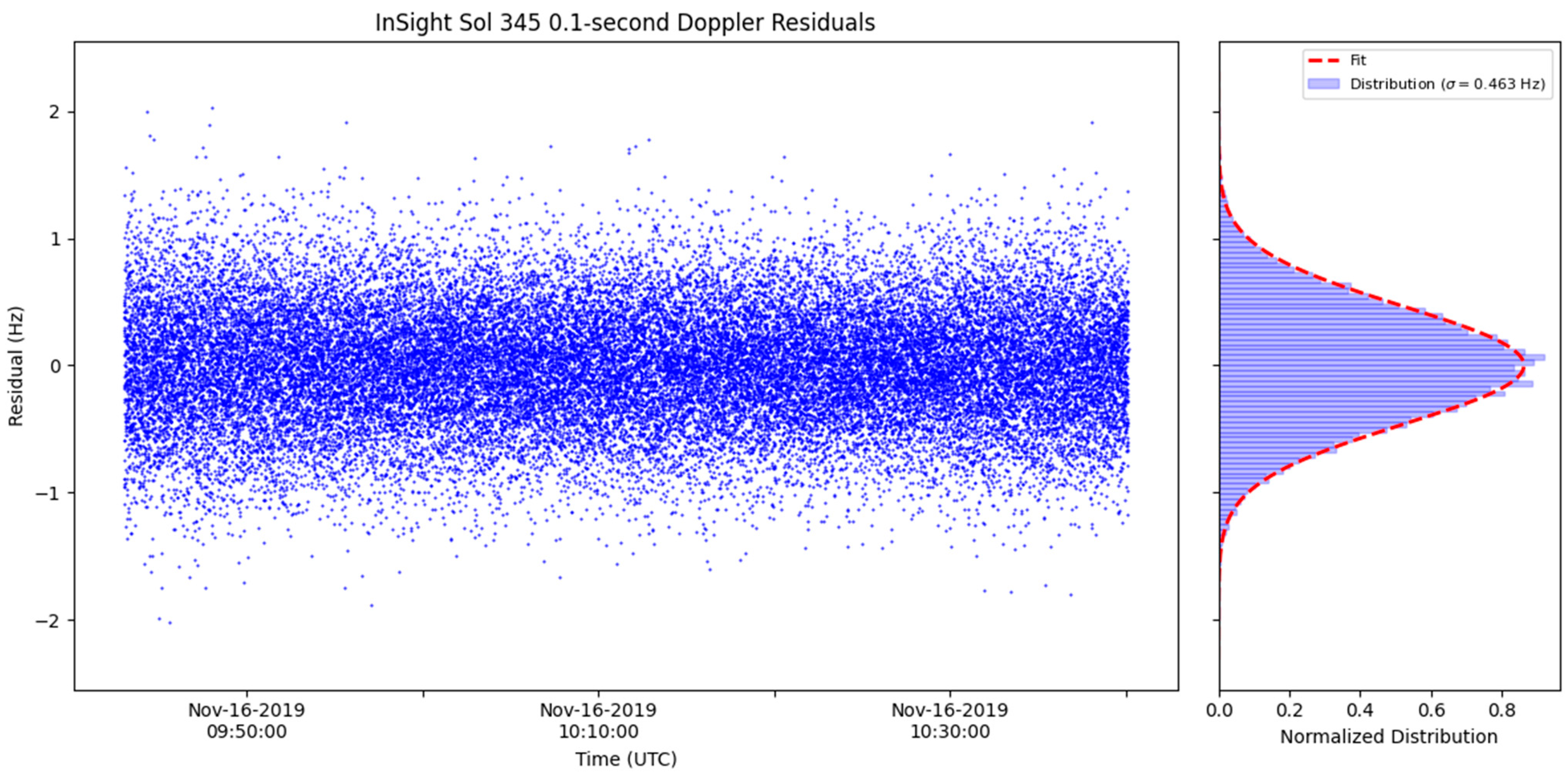
Doppler residuals at a count-time of 0.1 s from Sol 345 (16 November 2019) are shown in Figure 2 and are representative of a typical pass. The averaged carrier signal-to-noise ratio was 20.9 dB-Hz (linear scale 123 Hz, or SNR_V = 4.96), yielding a modeled thermal noise of 0.463 Hz (Equation (4)). The observed standard deviation of the Doppler residuals was 0.454 Hz, in good agreement with the model.

Figure 3 shows the Allan deviation computed from the Doppler residuals from the Sol 345 pass. Models of each noise behavior are fit to the Allan deviation curve. At low integration times, thermal noise is the dominant source, transitioning to troposphere noise at mid integration times, and finally, plasma-dominated noise at longer integration times.

For InSight analysis, a Doppler measurement count time of 60 s is used to provide several tens of points per 30–60 min tracking pass to look for signals from Mars rotation parameters that have a period near one Martian day [15]. When the dominant noise source is characterized as thermal (white phase noise), phase averaging is the optimal method to compress the Doppler data, because it optimizes all the signal-to-noise present in the phase. To reduce numerical noise, a model of the frequency is removed from the frequency observables before calculations are performed, resulting in these calculations being performed at the residual level. Firstly, the residual phase measurements are retrieved from the frequency residuals through integration. These can alternately be taken directly from the phase output of the BVR and the phase model removed. The first phase value, defined at a timestamp of t − T_c/2, is set to zero, and subsequent phase values are computed by adding the frequency multiplied by the count time to the previous phase value:

$$\varphi \left(t+\frac{T_c}{2}\right)=\varphi \left(t-\frac{T_c}{2}\right)+T_{c}f\left(t\right)$$

(5)

Sequential phase measurements are then averaged to yield a compressed phase observable time series:

$${\varphi }_c=\frac{{\varphi }_1+{\varphi }_2+\cdots +{\varphi }_n}{n}$$

(6)

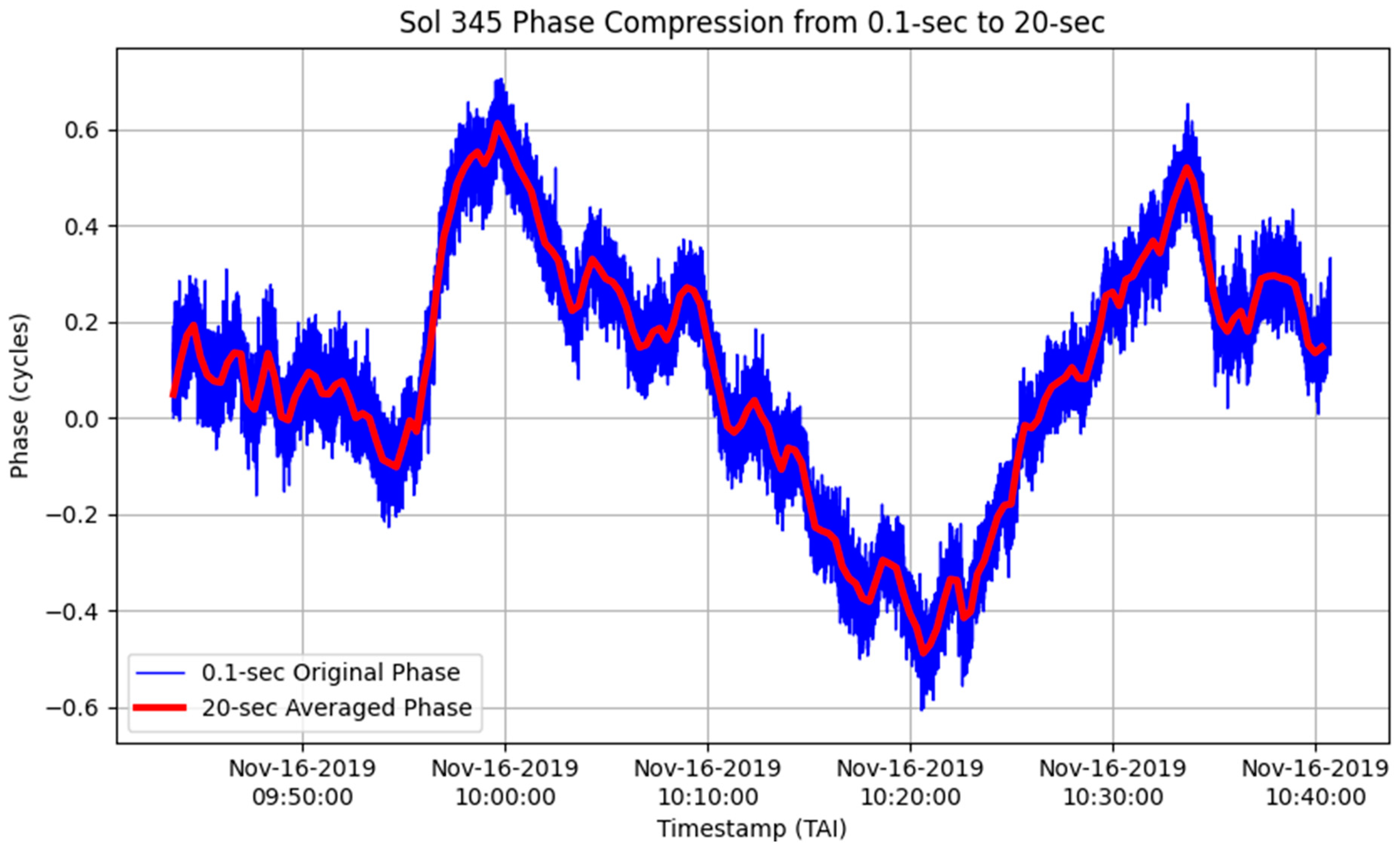
where ${\varphi }_c$ is the compressed phase, and n is the number of phase measurements averaged, equivalent to the ratio of the original count time to the desired count time (n = T_c,new/T_c,old). This is equivalent to performing a coherent phase average over a 20 s interval. The original 0.1 s and the 20 s averaged phase residuals are shown in Figure 4.

Frequency observables are then computed again from the phase time series by differencing adjacent phase values with Equation (1).

As seen in Figure 3b, the 0.1 s Doppler measurements are dominated by thermal noise for times shorter than ~20 s and by troposphere noise for time scales from ~20 s to 60 s. Although the exact crossover time between SNR noise and troposphere noise varies by a few seconds over the mission (due to change in SNR from Earth–Mars distance and change in SNR due to Earth being in different parts of the MGA antenna pattern for different geometries), for InSight, 20 s for phase averaging is used as the cutoff for all passes, since 20 s Doppler points can be conveniently averaged in frequency to give the standard 60 s points used in the analysis.

After phase compression from 0.1 s to 20 s, the dominant noise source is characterized as troposphere noise (white frequency noise), where typical frequency compression can be utilized.

$$f_c=\frac{f_1+f_2+\dots +f_n}{n}$$

(7)

Effectively, averaging the frequencies is equivalent to differencing the first and last phase points in the series. This can be proven by substituting Equation (1) into Equation (7). For example, averaging three data points (as performed for the compression from 20 s to 60 s count time in processing), the intermediate phase points cancel:

$$f_c=\frac{\left(-\frac{{\varphi }_1-{\varphi }_2}{T_{c,old}}\right)+\left(-\frac{{\varphi }_2-{\varphi }_3}{T_{c,old}}\right)+\left(-\frac{{\varphi }_3-{\varphi }_4}{T_{c,old}}\right)}{n}=-\frac{\left({\varphi }_1-{\varphi }_4\right)}{T_{c,new}}$$

(8)

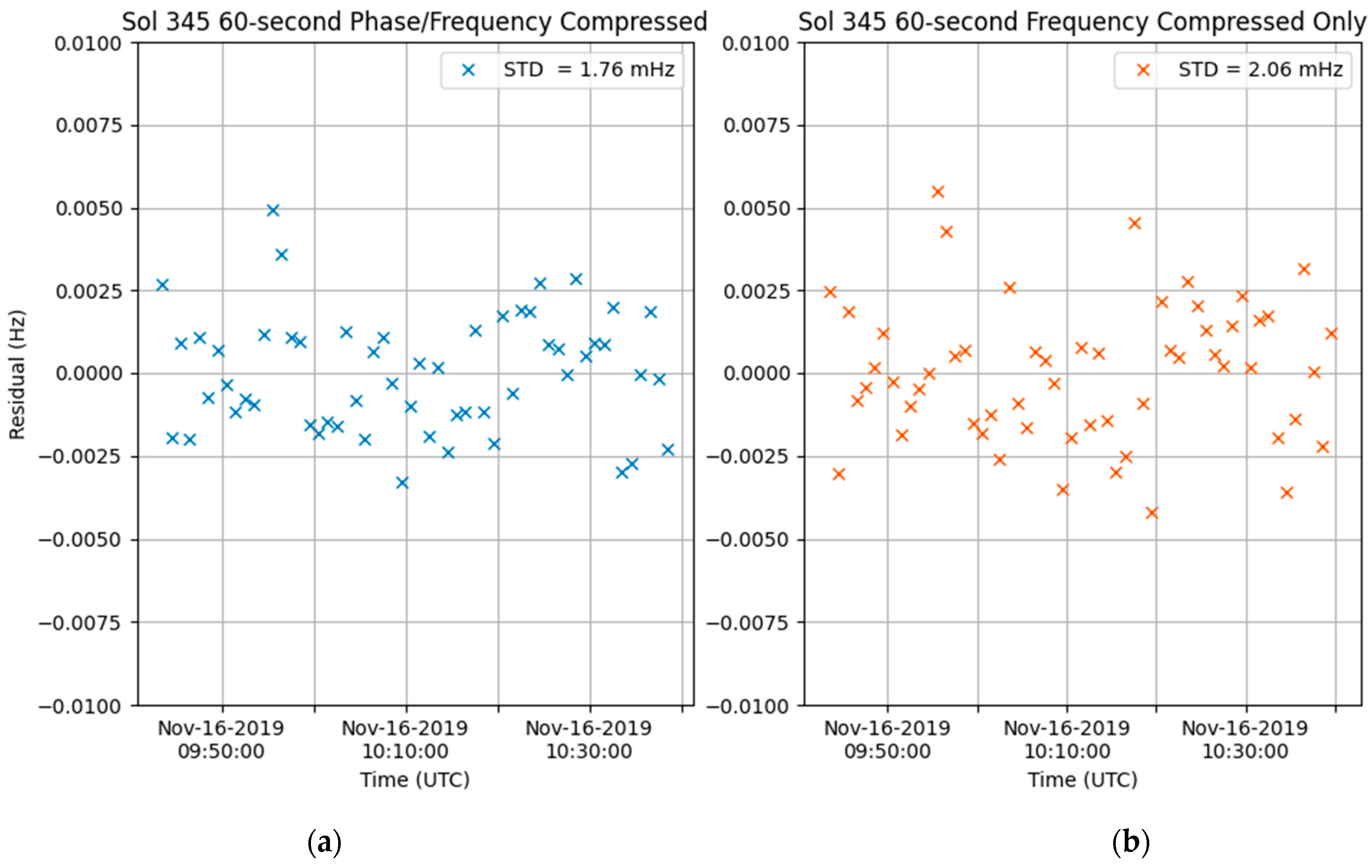
The 60 s count time Doppler residuals from the Sol 345 example are shown in Figure 5. Using the combined phase averaging from 0.1 s to 20 s count-time, followed by frequency averaging from 20 s to 60 s count time, yields a 60 s Doppler residual standard deviation of 1.76 mHz. If only frequency compression was used from 0.1 s to 60 s count time (as would be the case in the tracking data file if 60 s Doppler points were requested directly from the DSN), the Doppler residual standard deviation would be 2.06 mHz, an increase of 17%.

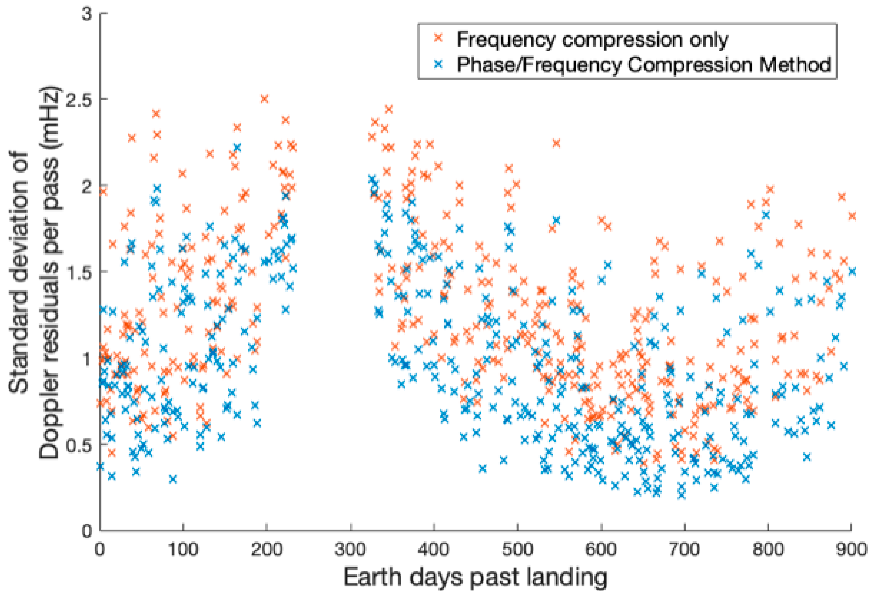
During the first 900 days of InSight data collection (spanning November 2018 to November 2021), a total of 578 Doppler tracking passes were executed. These varied in both signal-to-noise ratio and Sun–Earth–Probe angle. The standard deviation of the Doppler residuals in each pass is shown in Figure 6. The average improvement using the phase compression technique in the SNR-limited regime was 25%. If used in an orbit determination filter, as for InSight radio science analysis [15], any improvement in residual is proportional to the uncertainty of the measured parameters due to the linearization of the filter. Thus, without this data compression technique, the resulting uncertainties of the estimated parameters in the filter would be correspondingly ~25% larger, depending on data weighting and the linear behavior of the parameters.

5. Conclusions

The InSight radio science investigation utilized MGAs, which resulted in lower SNR than what would normally be received if using an HGA. The resulting radio Doppler measurements, received by the closed-loop receiver of the DSN, have higher thermal noise than those using an HGA due to their lower SNR. Optimal configuration of the DSN closed-loop receiver to match the loop bandwidth with the output rate and utilizing phase-averaging in the thermally limited measurement regime can reduce and eliminate the additional thermal noise caused by the lower SNR with the MGAs. For InSight, using this approach resulted in a 17% reduction in measurement noise for the Sol 345 pass and ~25% reduction in noise over the passes in the first 900 days of InSight data collection. This novel approach can be used by any radio science investigation using Doppler measurements from the DSN closed-loop receiver to improve the precision of the measurement. The only limitation of using this approach is that the closed-loop receiver must be able to lock to the signal. In the case when it is not possible to retain a lock with the closed-loop receiver, open-loop processing techniques can be used in conjunction with this approach.

References

- Deep Space Network. DSN Telecommunications Link Design Handbook; JPL: Pasadena, CA, USA, 2021. Available online: https://deepspace.jpl.nasa.gov/dsndocs/810-005/ (accessed on 2 January 2022).
- Kuchynka, P.; Folkner, W.M.; Konopliv, A.S.; Parker, T.J.; Park, R.S.; Le Maistre, S.; Dehant, V. New constraints on Mars rotation determined from radiometric tracking of the Opportunity Mars Exploration Rover. Icarus 2014, 229, 340–347. [Google Scholar] [CrossRef]
- Folkner, W.M.; Dehant, V.; Le Maistre, S.; Yseboodt, M.; Rivoldini, A.; Van Hoolst, T.; Asmar, S.W.; Golombek, M.P. The rotation and interior structure experiment on the InSight mission to Mars. Space Sci. Rev. 2018, 214, 1–16. [Google Scholar] [CrossRef]
- Dehant, V.; Le Maistre, S.; Baland, R.M.; Bergeot, N.; Karatekin, Ö.; Péters, M.J.; Rivoldini, A.; Lozano, L.R.; Temel, O.; Van Hoolst, T.; et al. The radioscience LaRa instrument onboard ExoMars 2020 to investigate the rotation and interior of mars. Planet. Space Sci. 2020, 180, 104776. [Google Scholar] [CrossRef]
- Mazarico, E.; Buccino, D.R.; Castillo-Rogez, J.; Dombard, A.; Genova, A.; Hussmann, H.; Kiefer, W.S.; Lunine, J.I.; McKinnon, W.B.; Nimmo, F.; et al. The Europa Clipper Gravity/Radio Science Investigation. In Proceedings of the Lunar and Planetary Science Conference, Online, 15–19 March 2021; p. 1784. [Google Scholar]
- Moyer, T.D. Formulation for Observed and Computed Values of Deep Space Network Data Types for Navigation; John Wiley & Sons: New York, NY, USA, 2005; Volume 3. [Google Scholar]
- Berner, J.B.; Bryant, S.H. New Tracking Implementation in the Deep Space Network. In Proceedings of the ESA 3rd Workshop on Tracking, Telemetry and Command Systems for Space Applications, Noordwijk, The Netherlands, 29 October 2001; Jet Propulsion Laboratory, National Aeronautics and Space Administration: Pasadena, CA, USA, 2001. Available online: https://trs.jpl.nasa.gov/bitstream/handle/2014/39284/01-1846.pdf?sequence=1&isAllowed=y (accessed on 2 January 2022).
- Stephens, S.A.; Thomas, J.B. Controlled-Root Formulation for Digital Phase-Locked Loops. IEEE Trans. Aerosp. Electron. Syst. 1995, 31, 78–95. [Google Scholar] [CrossRef]
- Asmar, S.W.; Armstrong, J.W.; Iess, L.; Tortora, P. Spacecraft Doppler tracking: Noise budget and accuracy achievable in precision radio science observations. Radio Sci. 2005, 40, 1–9. [Google Scholar] [CrossRef] [Green Version]
- Allan, D.W. Statistics of atomic frequency standards. Proc. IEEE 1966, 54, 221–230. [Google Scholar] [CrossRef] [Green Version]
- International Radio Consultative Committee. Characterization of Frequency and Phase Noise; International Radio Consultative Committee: Geneva, Switzerland, 1986; pp. 142–150. Available online: https://tf.nist.gov/general/tn1337/Tn162.pdf (accessed on 2 January 2022).
- Keihm, S.J.; Tanner, A.; Rosenberger, H. Measurements and calibration of tropospheric delay at Goldstone from the Cassini media calibration system. IPN Prog. Rep. 2004, 2004, 42–158. [Google Scholar]
- Woo, R.; Yang, F.C.; Yip, K.W.; Kendall, W.B. Measurements of large-scale density fluctuations in the solar wind using dual-frequency phase scintillations. Astrophys. J. 1976, 210, 568–574. [Google Scholar] [CrossRef]
- Buccino, D.R.; Kahan, D.S.; Parisi, M.; Paik, M.; Barbinis, E.; Yang, O.; Park, R.S.; Tanner, A.; Bryant, S.; Jongeling, A. Performance of earth troposphere calibration measurements with the advanced water vapor radiometer for the Juno Gravity science investigation. Radio Sci. 2021, 56, 1–9. [Google Scholar] [CrossRef]
- Kahan, D.S.; Folkner, W.M.; Buccino, D.R.; Dehant, V.; Le Maistre, S.; Rivoldini, A.; Van Hoolst, T.; Yseboodt, M.; Marty, J.C. Mars precession rate determined from radiometric tracking of the InSight Lander. Planet. Space Sci. 2021, 199, 105208. [Google Scholar] [CrossRef]
Figure 1.
Simplified block of the closed-loop Doppler measurement process.
Figure 2.
Doppler residuals at 0.1 s count-time for Sol 345 (left), and histogram distribution of the residuals (right). The standard deviation of the residuals is 0.463 Hz.
Figure 3.
(a) Power spectral density of 0.1 s residual frequency for the Sol 345 pass, showing the white phase noise dominance. (b) Allan deviation (fractional frequency stability) of the Sol 345 pass. Fits of the three primary noise component models (white phase noise, white frequency noise, and Kolmogorov noise) are shown.
Figure 4.
Residual phase at the original 0.1 s count-time and the resulting averaged phase residuals at a 20 s integration time for the Sol 345 pass.
Figure 5.
Doppler residuals at 60 s count-time for Sol 345 with two compression methods. Left (a), using phase compression from 0.1 s to 20 s using phase averaging followed by frequency compression from 20 s to 60 s; and right (b), using frequency compression from 0.1 s to 60 s only.
Figure 6.
Standard deviation of Doppler residuals at 60 s count time for all passes in the first 900 days of operations. Only the standard deviation of the described phase/frequency compression method and the traditional frequency compression are shown.
Publisher’s Note: MDPI stays neutral with regard to jurisdictional claims in published maps and institutional affiliations. |
© 2022 by the authors. Licensee MDPI, Basel, Switzerland. This article is an open access article distributed under the terms and conditions of the Creative Commons Attribution (CC BY) license (https://creativecommons.org/licenses/by/4.0/).
Share and Cite
MDPI and ACS Style
Buccino, D.; Border, J.S.; Folkner, W.M.; Kahan, D.; Le Maistre, S. Low-SNR Doppler Data Processing for the InSight Radio Science Experiment. Remote Sens. 2022, 14, 1924. https://0-doi-org.brum.beds.ac.uk/10.3390/rs14081924
AMA Style
Buccino D, Border JS, Folkner WM, Kahan D, Le Maistre S. Low-SNR Doppler Data Processing for the InSight Radio Science Experiment. Remote Sensing. 2022; 14(8):1924. https://0-doi-org.brum.beds.ac.uk/10.3390/rs14081924
Chicago/Turabian StyleBuccino, Dustin, James S. Border, William M. Folkner, Daniel Kahan, and Sebastien Le Maistre. 2022. "Low-SNR Doppler Data Processing for the InSight Radio Science Experiment" Remote Sensing 14, no. 8: 1924. https://0-doi-org.brum.beds.ac.uk/10.3390/rs14081924
Note that from the first issue of 2016, this journal uses article numbers instead of page numbers. See further details here.