A Numerical Investigation of the Dispersion Law of Materials by Means of Multi-Length TDR Data


1
Department of Environmental Engineering DIAM, University of Calabria, 87036 Rende, Italy
2
Department of Physics, University of Malta, 2080 Msida, Malta
*
Author to whom correspondence should be addressed.
Remote Sens. 2022, 14(9), 2003; https://0-doi-org.brum.beds.ac.uk/10.3390/rs14092003
Submission received: 27 January 2022
/
Revised: 13 April 2022
/
Accepted: 15 April 2022
/
Published: 21 April 2022
(This article belongs to the Special Issue Latest Results on GPR Algorithms, Applications and Systems)
Abstract
:In this paper, we propose a method for retrieving the dispersion law of a material under test from multi-length TDR measurements in reflection mode, repeated at several frequencies. By replacing the multi-frequency measurements with measurements using multi-length TDR probe, it is possible to retrieve the complex equivalent permittivity of the material in a frequency band of interest. The proposed procedure does not require a priori knowledge of the type of dispersion law of the material, which instead can possibly be inferred from the measured data. The algorithm is validated using numerically simulated data obtained with the commercial code CST Microstudio®.
1. Introduction
Time domain reflectometry (TDR) probes offer a procedure for measuring the electromagnetic properties of a material under test (MUT) through the measurement of the electromagnetic field reflected from it or also (more rarely) transmitted through it [1]. In particular, TDR is an important tool supporting the data processing and interpretation of ground penetrating radar (GPR) data. In fact, in these cases, obtaining information about the characteristics of the medium embedding the buried targets requires a correct time–depth conversion and an optical focusing of the buried objects [2,3]. Other complementary methods exist that are based on the same GPR data and data values averaged on a large portion of the subsoil. However, these methods rely on some assumptions that may not always be correct and/or require expensive equipment [4].
The theory of transmission lines, and more in general, that of waveguides, is at the basis of the measurement of material properties such as the dielectric permittivity (possibly complex to account for losses), the electrical conductivity, and the magnetic permeability of the MUT [5,6]. Beyond common GPR applications, the possible uses of this technology and methodology range from biomedical applications [7] to pollution detection [8], alimentary checks, diagnostics of electric networks, monitoring of buried subservices [9,10], and a very common application related to the water content in soil [11,12,13].
In its easiest (and perhaps most common) application, TDR probes are employed to deduce the propagation velocity of the waves in a MUT from the return time of a pulsed or constant level wave launched along the rods of the probe. However, this intrinsically obliterates the dependence on the frequency of the electromagnetic characteristics of the MUT, yielding only average values. Therefore, in the early works of Nicholson and Ross (1970) and Weir (1974)(refs. [5,6]), the dielectric characteristics of a MUT were retrieved in the frequency domain from the measured S-parameters of a sample of the MUT inserted in a rectangular waveguide. Subsequently, based on the same principle (but only in reflection mode for practical reasons), the S11 parameter retrieved from a TDR probe and its relationship with the permittivity of the medium were considered, in most cases, matching the least square sensed data with a model, characterized by a few (frequency independent) parameters based on a predetermined dispersion law, for example, in [14]. This allows us to exploit the frequency dependence in order to gain more information about the parameters of a pre-chosen dispersion model such as the Deybe, with one or more relaxation times, Cole–Cole, Maxwellian, or Q-constant dispersion laws [15,16].
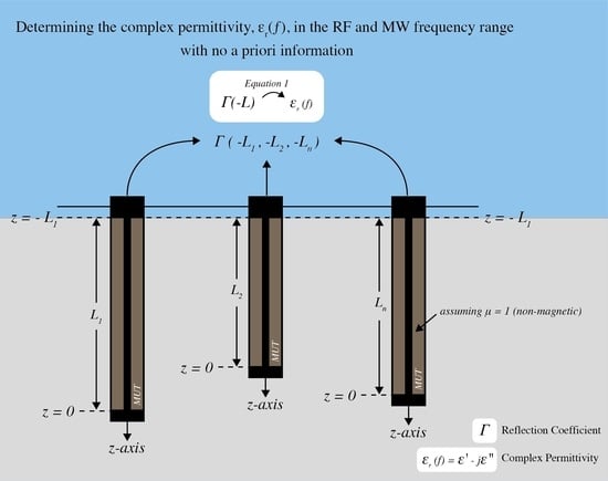
In this paper, we will try to overcome the constraint of a predetermined dispersion model, and will focus on the measurement of the dispersion law of a non-magnetic material. In particular, most natural materials are indeed non-magnetic in the radiofrequency and microwave frequency range, with few exceptions [17], and in any case, the possible presence of magnetic properties of the MUT can be tested with preliminary measurements [18,19]. Overcoming the constraint of a pre-assumed dispersion law allows one to characterize any new and unknown MUT (e.g., an artificial material created for a specific purpose and never examined before, or in cases when the physico-chemical characteristics of the material are not precisely known, or in case when the inclusions of impurities can change the dispersion law in an unforeseen way).
This work introduces a new method for dielectric properties retrieval through “length diversity” by means of probes with a different length of conductors along which the TDR signal propagates. This will result in obtaining more information at any fixed frequency in the band of interest.
Moreover, multi-length data do not change the electrical cross-section of the probe at the considered frequency and do not introduce the possibility of higher order propagation modes [20], which could instead happen when progressively increasing the frequency in a probe of fixed length. On the other hand, multi-length measurements are intrinsically more time consuming, and in particular, their execution requires either dedicated hardware where a TDR probe can somehow be progressively prolonged, or alternatively, an array of probes with the same cross section, same input connections, and same termination but with different lengths. This means that a multi-length probe would be more expensive than a common TDR probe. To the best of our knowledge, multi-length TDR probes are not available on the market, presumably just for the said reasons. In this study, a multi-length probe was simulated using CST Microwave Studio by means of sequential numerical experiments with a progressively longer probe. This commercial code is based on the method of finite difference in the time domain FDTD [21]. This software allows for simulation of the electromagnetic fields and, consequently, the S-parameters of any guiding structure. In particular, a coaxial cable terminated with a shunt was considered. Data considered consisted of the reflection coefficient at the beginning of a piece of coaxial cable filled with the MUT and terminated with a short circuit between the two conductors of the cable. This reflection coefficient was evaluated for several lengths of the final part of the coaxial cable (that is, filled up with the MUT) at fixed frequency, so the characteristics of the material at that frequency were evaluated from single frequency (but multi-length) measurements. Then, the same procedure was repeated at other frequencies (progressively increased with a uniform frequency steps) to retrieve the dispersion law within the prefixed frequency band of interest. This means that the comprehensive considered data are indeed multi-length and multi-frequency, whereas the processing is based on a multi-length inversion sequentially applied to several single-frequency data.
2. Mathematical Model
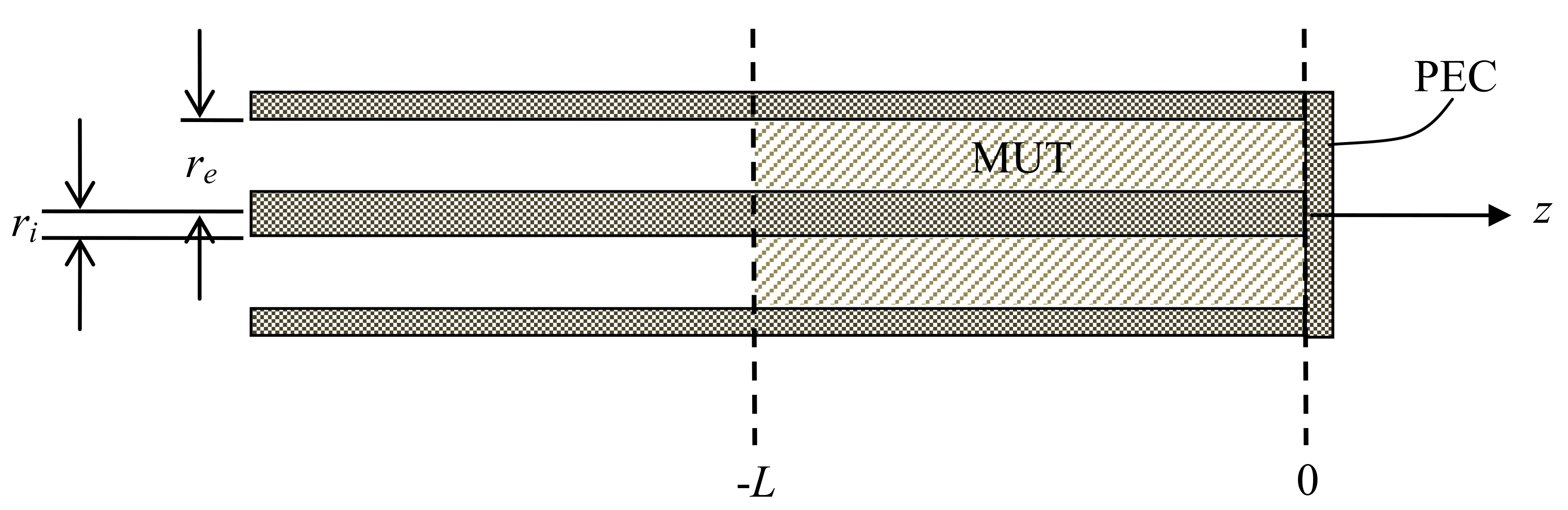
The reference model used in this study is represented in Figure 1. The MUT fills the last part of a coaxial cable that is terminated with a perfect electric conductor (PEC) and is fed from the opposite end. The part that hosts the MUT extends from the abscissa –L up to the abscissa 0, according to the reference system usually adopted for transmission lines, where the zero occurs at the load and the generator is placed at a negative abscissa [20].
The datum is the reflection coefficient at z = −L, that is, a point of discontinuity for the reflection coefficient along the line. The unknown of the problem is the relative complex equivalent permittivity of the MUT εr = εr′ − jεr″, where both εr′ and εr″ are real and positive with εr′ ≥ 1. The relative magnetic permeability of the MUT is assumed to be equal to 1.
Starting from the well-known theory of transmission lines, with some algebra, the reflection coefficient Γ at in Figure 1 is given by:
where is the intrinsic impedance of the length L of coaxial line hosting the MUT, evaluated when empty. It is independent of the unknowns and is given by [20]:
where and are respectively the radius of the internal and the external conductors of the coaxial cable; ε0 = 8.854 × 10⁻¹²; Fm−1 is the permittivity; and μ0 = 1.256 × 10⁻⁷ Hm−1 is the permeability of free space.
is the intrinsic impedance of the part of the cable before the reference plane (i.e., ) and is the propagation velocity of electromagnetic waves in free space.
Regarding the determination of the complex square root of the unknown relative permittivity, it has to have a positive real part and negative imaginary part. In particular, this means that the energy of the waves vanishes exponentially far from the source, being progressively transformed into heat.
The problem amounts to retrieving the two real unknowns εr′ and εr″ from the measured reflection coefficient data by inverting Equation (1). Considering multi-length data at fixed frequency, this can be conducted by minimizing a cost function expressed as:
where and ; is the reflection coefficient measured at the kth length (keeping the frequency fixed) of the coaxial line filled with the MUT, and is the modeled reflection coefficient for , provided by Equation (1). The cost function is not quadratic because the link between the unknowns and the data is nonlinear. This means that in general, local minima are expected [22], but this is not particularly troublesome because only two unknowns are looked for. In particular, it is possible to make use of an exhaustive minimization algorithm to overcome the problem of the local minima. However, in the lossless case, the cost function also exhibited a periodicity with α, which generated several global minima. This can generate a misinterpretation of the data, even in a low-loss case with noisy data. As shown in [18], the problem can be overcome if the length step respects the following condition:
where is the fixed frequency and is the range of variability (necessarily pre-chosen) within which we look for the value of α.
3. Results
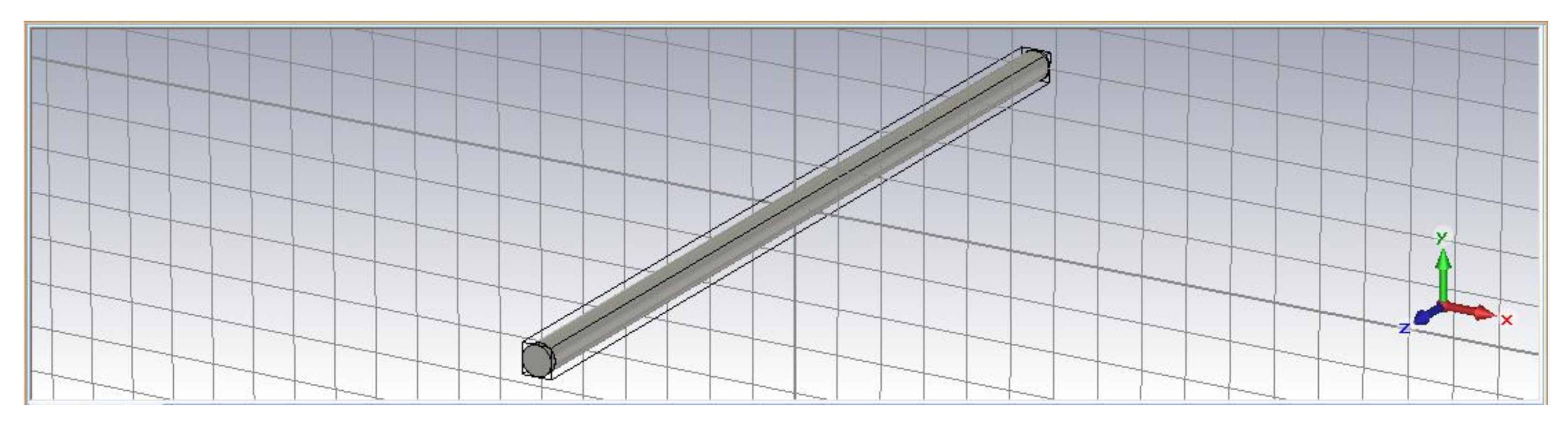
A coaxial cable was modeled using the CST Microwave Studio, as shown in Figure 2. The cable input port was excited at one end using a 50 ohm impedance port. This is equivalent to an incident wave coming from a coaxial cable with an intrinsic impedance of 50 ohms. The coaxial cable that hosts the MUT has an internal radius of 1.7 mm and an external radius of 5.7 mm. This means that when no MUT is inserted in the coax, its intrinsic impedance is equal to 72.54 ohms. The other end of the coaxial cable is shunted. The reflection coefficient at the port is evaluated in the frequency band 500–1000 MHz (this particular frequency range is relevant for GPR applications), spanned with a frequency step of 25 MHz. The simulation was repeated 21 times, each time changing the length of the coax, starting from 20 up to 40 cm with a length step of 1 cm. In particular, the electric field was simulated at each frequency of interest, in order to obtain a more precise evaluation of the reflection coefficient at that frequency (as well known, it is possible to evaluate the electric field at one frequency and then extract the scattering parameters at several frequencies from that).
With these 21 numerical experiments, 21 vector data were obtained, each representing the reflection coefficient as a function of frequency at any fixed length of the cable. Combining all these data as a column of a matrix, it is obvious that the rows of the matrix represent the reflection coefficient as a function of the length of the cable at any fixed frequency. In this way, we simulated multi-length data at each considered frequency.
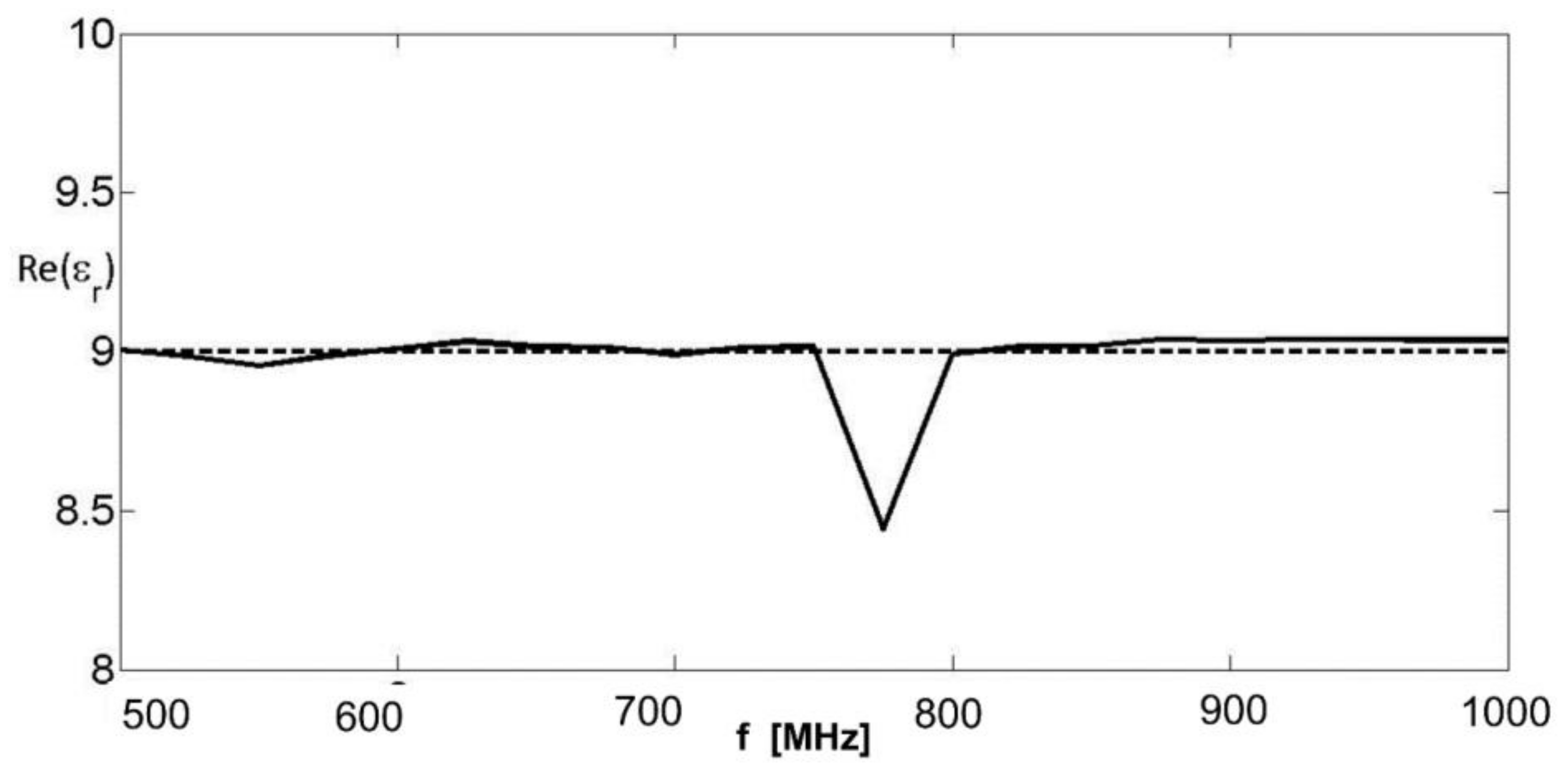
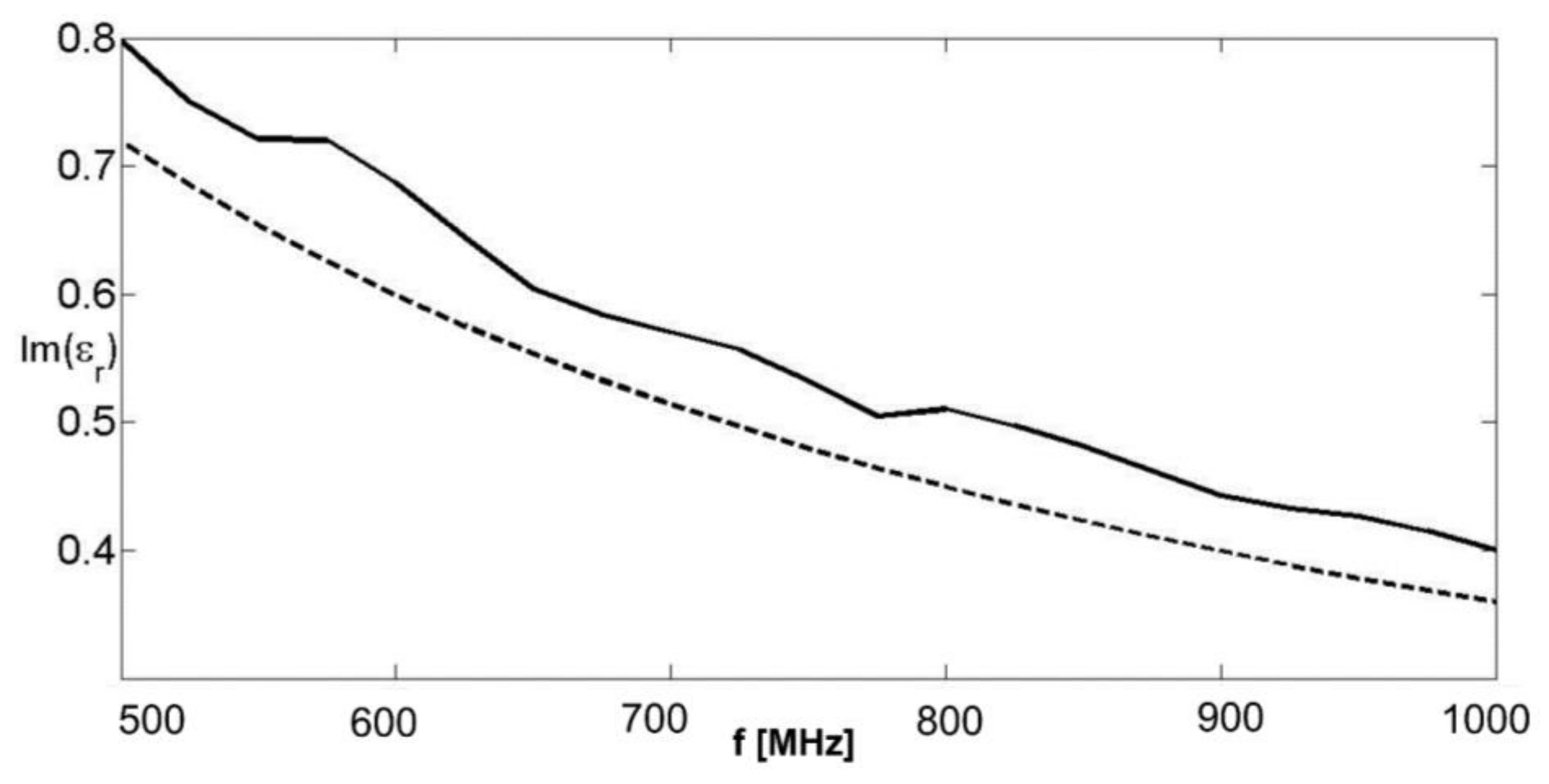
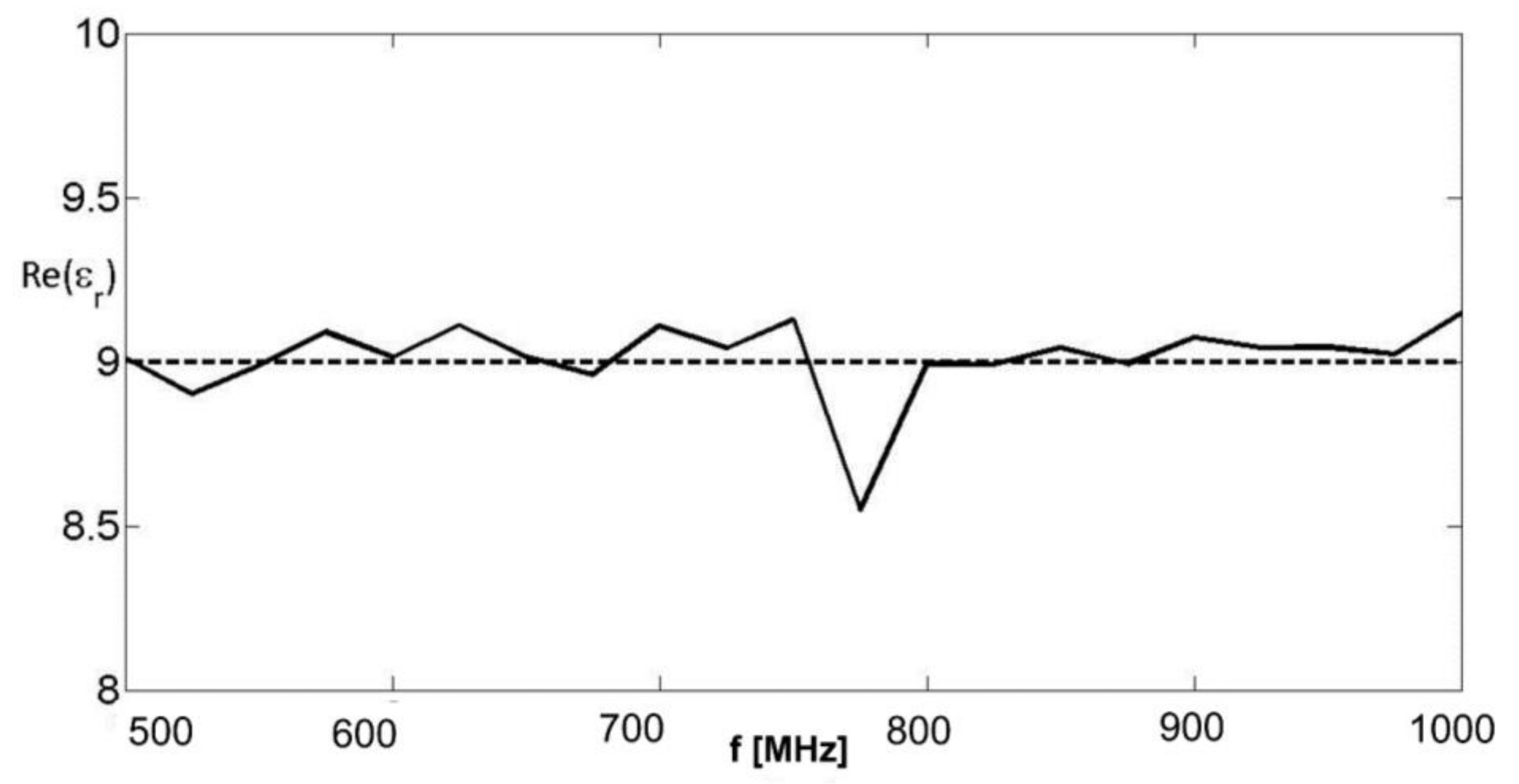
The MUT follows a Maxwellian dispersion law, with relative dielectric permittivity = 9 and electric conductivity = 0.02 Sm−1. Therefore, its equivalent complex relative permittivity is equal to , where is the absolute dielectric permittivity of free space and f is the frequency. The multi-length data at each frequency were inverted, looking for two parameters, namely the real and imaginary parts of the square root of the equivalent complex dielectric permittivity . In particular, in this case, the real part of the complex relative permittivity is constant with frequency, whereas the imaginary part vanishes hyperbolically with frequency.
The inversion algorithm is iterative and exhaustive at each step. At the first step, the intervals of values [1, 20] and [–4, 0], both sampled with 801 uniformly spaced samples, are combined in a matrix of values that is spanned sequentially. After the first minimization, the procedure is iterated on a rectangular investigation domain zoomed about the solution found at the previous step, again discretized with 801 × 801 points. The zoom was achieved considering one half of the extensions of the edges of the rectangle considered at the previous step, with the further physical constraint that the real part of the dielectric permittivity is not smaller than 1 (as for most of materials excluding plasmas) and the imaginary part is negative (which means that the medium is passive and does not generate electromagnetic energy). The iterations were four at most, but they stopped sooner if the minimum value of the cost function found at the nth step was larger than the homologous quantity found at the (n − 1)th step. If all four iterations were performed, a further check on the discrepancy between the results achieved at the third and fourth steps was conducted. In particular, if this discrepancy is large (5% or more), it means that the algorithm is still far from convergence and more iterations are required. However, in the cases shown in the study, the discrepancy was always smaller than 1%. In Figure 3 and Figure 4, the reconstructed real and imaginary parts (in modulus) of the reconstructed complex relative permittivity are shown as a function of frequency, together with the actual values represented with dashed lines. It can be seen that the real part was reconstructed very well all over the band, apart from a slightly higher discrepancy at 775 MHz. The retrieved imaginary part was slightly overestimated but followed quite well the frequency behavior of the actual value.
The reason for this bias is not yet fully understood, but the least square error on the real part of the relative dielectric permittivity as a function of frequency with respect to the actual value was equal to 1.4%, whereas the homologous error on the imaginary part was 12%. The comprehensive error on the complex relative permittivity was 1.5%. At this point, we can think of a further step inferring the type of dispersion law if the achieved result allows this. In particular, we can compare the achieved dispersion curve with the behavior of a pre-determined dispersion law, minimizing the discrepancy between the achieved dispersion curve and a pre-chosen dispersion model (e.g., a Maxwellian, Deybe, Cole-Cole, CRIM, etc.) at variance of the parameters characterizing the dispersion model chosen for the comparison. In the case at hand, from the achieved dispersion curve, it was adequate to choose a Maxwellian law for the parameter matching and such a least square optimization provided an estimated relative permittivity equal to 8.98 (which means an error of 0.22% with respect to the actual value) and an estimated electrical conductivity equal to 0.022 S/m (with an error of 10% with respect to the actual value). As can be seen, these errors were smaller than the least square errors between the achieved and actual dispersion laws, because we exploited some extra-information about the kind of dispersion law assumed for the MUT. In general, one might try different matching with different dispersion models and choose one that allows for the best matching with the achieved dispersion curve.
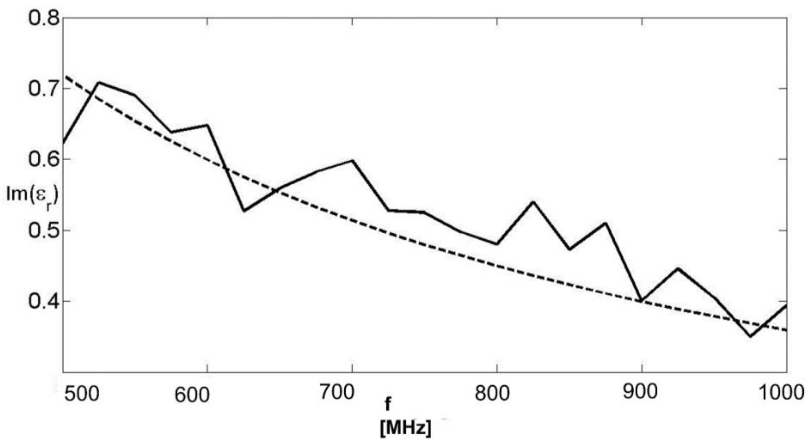
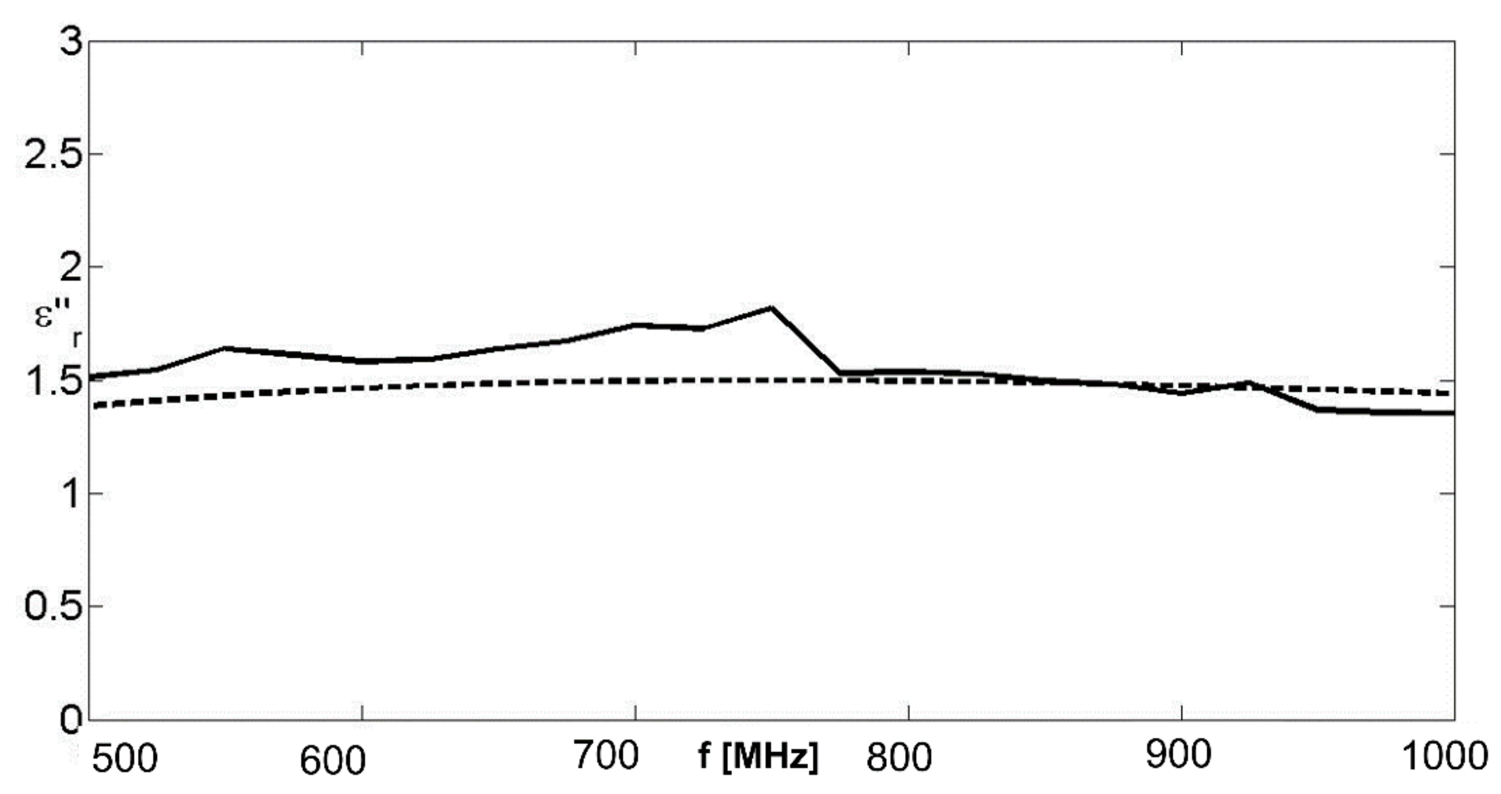
Figure 3 and Figure 4 refer to noiseless data. In order to test the robustness of the algorithm in the presence of noise, Gaussian white noise was added separately to the real and imaginary part of the data at each frequency. The signal to noise ratio was 10 dB in all cases. The results are represented in Figure 5 and Figure 6.
The least square error on the real part of the relative dielectric permittivity was 1.33%, the homologous quantity that referred to the imaginary part was 10.4%, and the error on the complex equivalent relative permittivity was 1.45%. Imposing a Maxwellian law, the best matching parameters were a relative permittivity equal to 9.01 and a conductivity equal to 0.021 S/m. As can be seen, the results were essentially the same achieved with noiseless data.
Let us now consider an example where the MUT follows a Deybe dispersion law [15], whose basic mathematical law (with a single relaxation time) is given by
where is the limit value of the relative permittivity at low frequency; is the limit value at very high frequency; and τ is the relaxation time of the material under test. , , and τ are real, positive parameters, and for the case at hand, we chose the values of , , and .
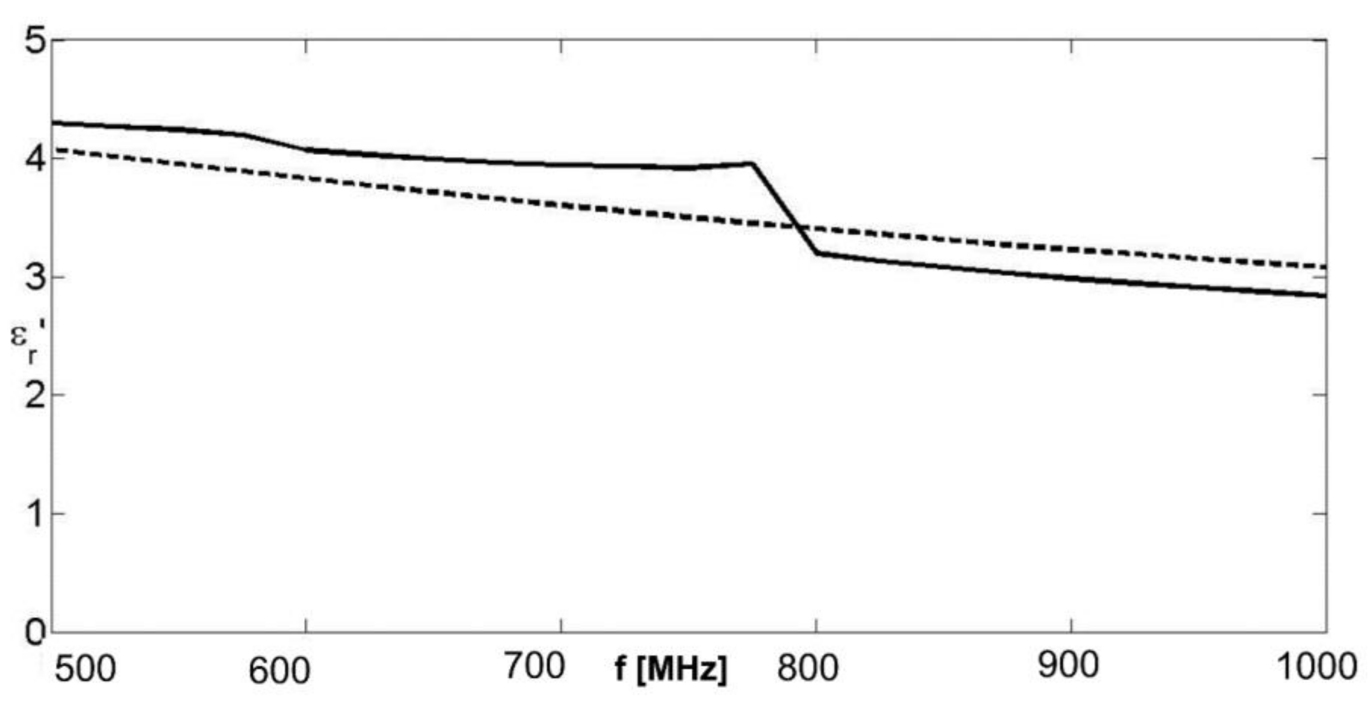
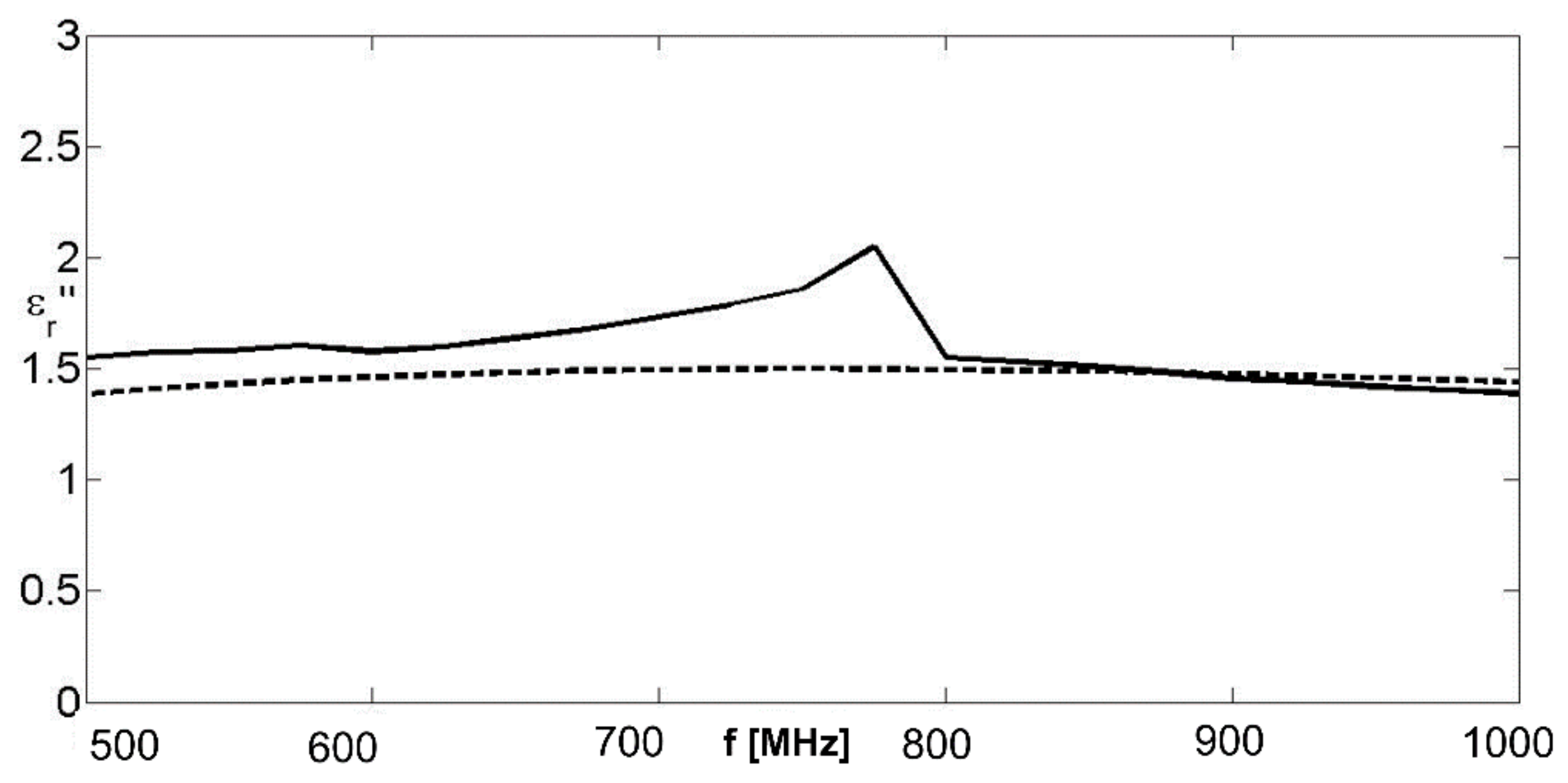
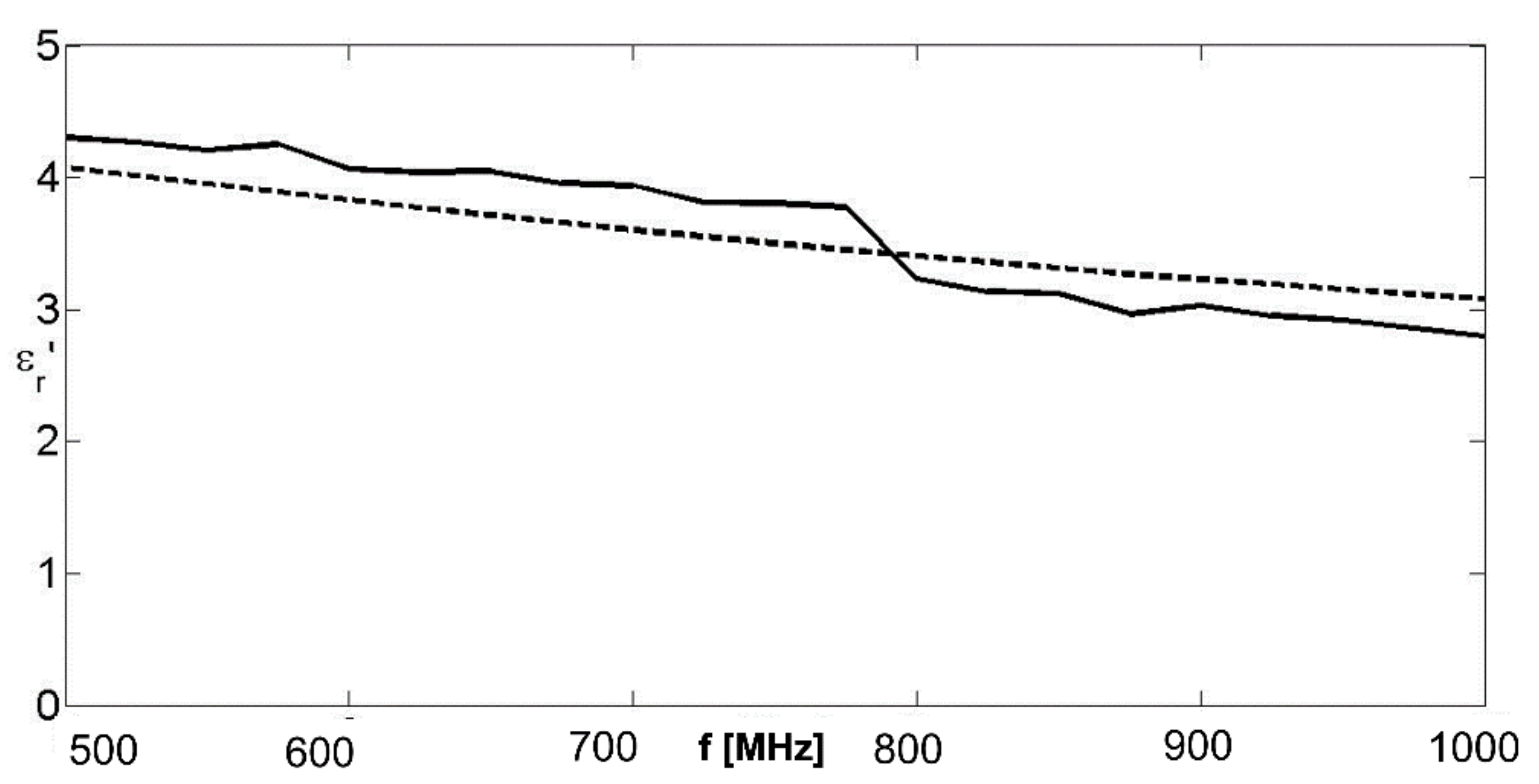
The coaxial cable was the same used for the previous example, and the exploited lengths were identical. The dispersion law was also investigated in the band 500–1000 MHz. Figure 7 and Figure 8 present the real and imaginary parts of the relative permittivity.
If a piece of prior information about the type of dispersion law is available, or if the type of dispersion law is deducible from the achieved results, then the least square matching between the achieved results and the assumed dispersion law at a variance of the three parameters , , and can be performed. In this case, the minimum of a cost function given by Equation (6) was considered,
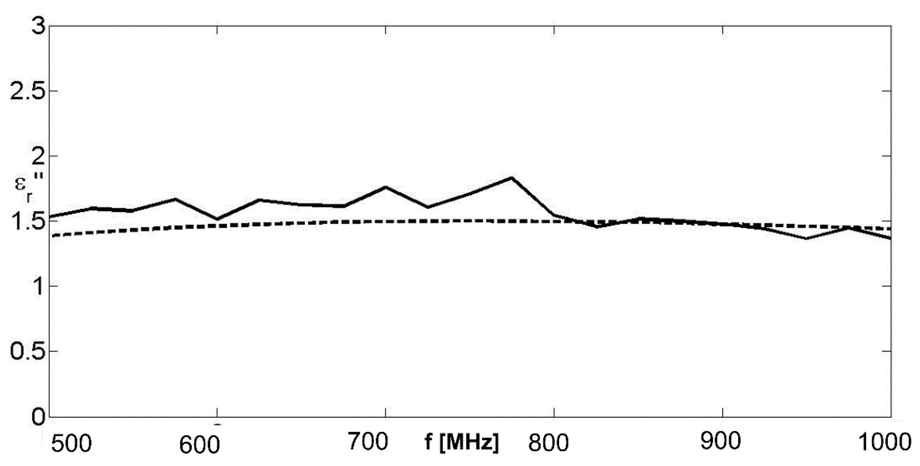
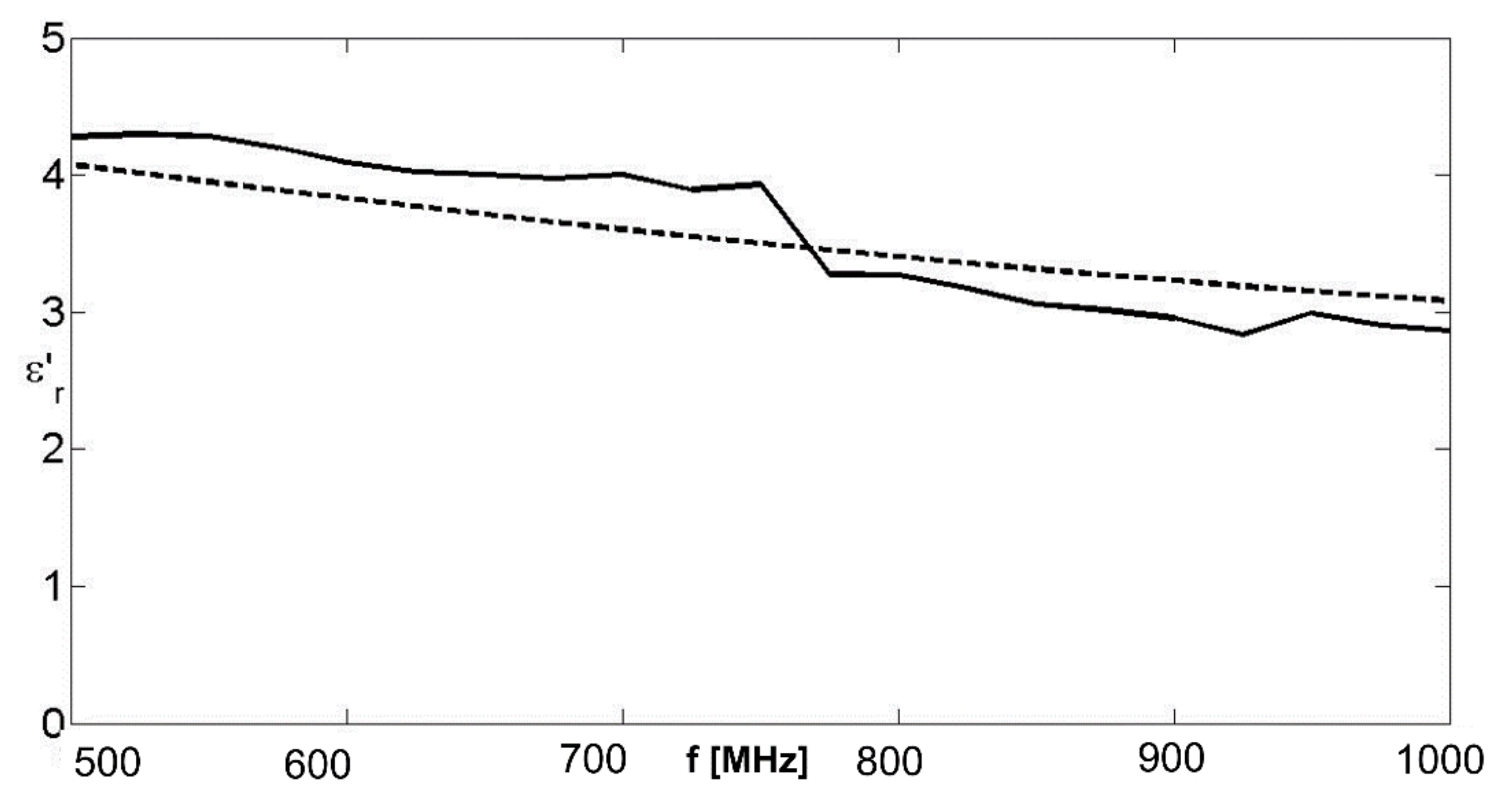
where is the assumed model for the relative permittivity, considered at the nth test frequency (in the case of an assumed Debye model, M is given by Equation (5)) and is the retrieved relative permittivity at the same frequency. In order to perform the minimization of the cost functional , an exhaustive minimization was used, making the trial value of range from 3 to 6, the trial values of range from 1 to 4, and the trial value of range from 0.1 to 0.3 ns. Regarding the choice of ranges, the values reached by the low and high frequency side by the real part of the retrieved relative permittivity can help with regard to and . With regard to τ, it is an easy exercise (starting from Equation (5)) to show that the imaginary part of the relative permittivity should reach its maximum value at the frequency , which immediately provides a first estimate of the relaxation time given by . In our case, the maximum of the imaginary part of the retrieved relative permittivity was reached at , which provides the first estimation . Therefore, it was natural to adopt a range centered on this value for the minimization. Each range was discretized with 501 points, so the comprehensive minimization was performed on 5013 = 125,751,501 points. The least square minimization provided the results , , and , with a percentage error of 8.8% on , 4.5% on , and 12.74% on . The agreement with the actual simulated values was not perfect, but the dispersion law was observed on a relatively narrow frequency band. In particular, the dispersion law observed on a wider band would immediately provide a more precise idea about and , these values being the limits of the real part for low and high frequencies. The results of Figure 6 and Figure 7, and consequently the least square matching of the dispersion parameters, were achieved with noiseless data. Figure 9 and Figure 10 represent the results obtained by adding white Gaussian noise to the data, as was conducted for the case of the Maxwellian dispersion law. A good robustness of the algorithm could be observed. The least square matching on the dispersion parameters in this case resulted in , , and , with an error of 8.2% on , 6.5% on , and 14.6% on .
As a further step to assess the robustness of the proposed method, we tested the sensitivity of the results vs. an error in the lengths of the multi-length probe. The numerical experiment was the same as that depicted in Figure 9 and Figure 10. However, the present evaluation involves white noise with SNR = 20 dB and a stochastic error on the length of the rods. This error is Gaussian with a standard deviation of 0.2 mm.
4. Conclusions
In this paper we proposed an algorithm to retrieve the dispersion law of a material under test within a prefixed range of frequencies, making use of TDR multi-length data. We focused on the case of a coaxial cable shunted at the end but other cases can also be considered such as changing the termination (open or matched coaxial cables), type of line (bifilar or trifilar TDR probes), or even the type of measurement device (waveguide). From the applicative point of view, a shunted coaxial cable can be particularly suitable in some biomedical applications, where the material to be investigated is liquid, semi-solid, or in powder form. The multi-length data can be acquired by sequentially setting pieces of probes of different lengths filled up with the MUT and attaching them to the same “generator” or making use of an array of different length probes with the same characteristics (in particular, also making use of an equivalent array of “generators”). With respect to waveguide measurements, a coaxial cable does not insert its own modal dispersion on the data if operated below the cut-off frequency of the first higher order propagation mode. The proposed model, exploiting only data gathered in reflection mode, is theoretically easily extendable to the case of bifilar or trifilar TDR probes. However, the latter configurations are not expected to be well described by a transmission line model because of the stronger effects of higher order modes. Nevertheless, calibration techniques could be devised, but these were beyond the scope of this introductory work.
The multilength approach is based, of course, on the assumption that the different probed samples of MUT are homogeneous and similar with respect to their dielectric properties. This hypothesis is reasonable in many cases, and in almost any case tested. In particular, different samples of powdered soil (gathered from the same region) should show a visibly different color and/or granularity if they are chemically or physically different from each other.
A last consideration is deserved about the effect of geometrical imprecisions in the coaxial cable. In particular, these are expected to be partially amortized by the logarithmic behavior of the intrinsic impedance of the line (see Equation (2)). In particular, if, for example, the size of the inner radius of the cable in the reported examples was 0.5 mm larger than its nominal value of 1.7 mm (which would mean a geometrical imprecision of 7%), then the intrinsic impedance of the line would change from 72.54 to 70.80 ohms (with an error of 2.4%).
The potential applications of the multilength approach are several because the dispersion law can constitute a sort of signature of the probed material that might reveal, for instance, the presence of some polluting substances in geophysical applications as well as the presence of toxic substances (in agricultural soils and natural underground water catchments) that are not easily identifiable with other methods.
Future works will also focus on an investigation of the “degrees of freedom” of the problem, looking for an optimal number of multilength measurements.
Author Contributions
Conceptualization, R.P.; Methodology, C.S. and L.F.; Software, I.F.; Validation, I.F. and R.P.; Formal analysis, R.P., C.S., and L.F.; Investigation, I.F.; Resources, L.F.; Data curation, I.F.; Writing—original draft preparation, R.P.; Writing—review and editing, L.F. and C.S.; Visualization, I.F.; Supervision, C.S.; Project administration, L.F.; Funding acquisition, L.F. All authors have read and agreed to the published version of the manuscript.
Funding
This research was funded by the Energy and Water Agency of Malta. The number of the funding is E20LG1.
Data Availability Statement
This study is based on simulated data, made available on request.
Acknowledgments
This work was discussed and developed within the European network Cost Action CA17115 “MyWAVE” and supported through the WetSoil project funded by the Energy and Water Agency in Malta.
Conflicts of Interest
The authors declare no conflict of interest.
References
- Gorriti, A.G.; Slob, E. A New Tool for Accurate S-Parameters Measurements and Permittivity Reconstruction. IEEE Trans. Geosci. Remote Sens. 2005, 43, 1727–1735. [Google Scholar] [CrossRef]
- Pierri, R.; Leone, G.; Soldovieri, F.; Persico, R. Electromagnetic inversion for subsurface applications under the distorted Born approximation. Nuovo Cimento C 2001, 24, 245–261. [Google Scholar]
- Catapano, I.; Crocco, L.; Persico, R.; Pieraccini, M.; Soldovieri, F. Linear and Nonlinear Microwave Tomography Approaches for Subsurface Prospecting: Validation on Real Data. IEEE Trans. Antennas Wirel. Propag. Lett. 2006, 5, 49–53. [Google Scholar] [CrossRef]
- Persico, R.; Ciminale, M.; Matera, L. A new reconfigurable stepped frequency GPR system, possibilities and issues; applications to two different Cultural Heritage Resources. Near Surf. Geophys. 2014, 12, 793–801. [Google Scholar] [CrossRef]
- Nicolson, A.M.; Ross, G.F. Measurement of the intrinsic properties of materials by time domain techniques. IEEE Trans. Instrum. Meas. 1970, 19, 377–382. [Google Scholar] [CrossRef] [Green Version]
- Weir, W.B. Automatic measurement of complex dielectric constant and permeability at microwave frequencies. Proc. IEEE 1974, 62, 33–36. [Google Scholar] [CrossRef]
- Cataldo, A.; Cannazza, G.; De Benedetto, E.; Giaquinto, N.; Trotta, A. Reproducibility analysis of a TDR-based monitoring system for intravenous drip infusions validation of a novel method for flow-rate measurement in IV infusion. In Proceedings of the 2012 IEEE International Symposium on Medical Measurements and Applications Proceedings, Budapest, Hungary, 18–19 May 2012; pp. 1–5. [Google Scholar]
- Menon, M.; Hermle, S.; Günthardt-Goerg, M.S.; Schulin, R. Effects of heavy metal soil pollution and acid rain on growth and water use efficiency of a young model forest ecosystem. Plant Soil 2007, 297, 171–183. [Google Scholar] [CrossRef]
- Cataldo, A.; De Benedetto, E.; Cannazza, G. Broadband Reflectometry for Enhanced Diagnostics and Monitoring Applications; Springer: Berlin/Heidelberg, Germany, 2011. [Google Scholar]
- Cataldo, A.; Persico, R.; Leucci, G.; De Benedetto, E.; Cannazza, G.; Matera, L.; De Giorgi, L. Time domain reflectometry, ground penetrating radar and electrical resistivity tomography: A comparative analysis of alternative approaches for leak detection in underground pipes. NDT & E Int. 2014, 62, 14–28. [Google Scholar]
- Topp, G.C.; Davis, J.L.; Annan, A.P. Electromagnetic, determination of soil water content: Measurements in, coaxial transmission lines. Water Resour. Res. 1980, 16, 574–582. [Google Scholar] [CrossRef] [Green Version]
- Zegelin, S.J.; White, I.; Jenkins, D.R. Improved fields probes for soil water content and electrical conductivity measurements using TDR. Water Resour. Res. 1989, 25, 2367–2376. [Google Scholar] [CrossRef]
- Moret, D.; Lopez, M.V.; Arrue, J.L. TDR application for automated water level measurement from Mariotte reservoirs in tension disc infiltrometers. J. Hydrol. 2004, 297, 229–235. [Google Scholar] [CrossRef] [Green Version]
- Cataldo, A.; Catarinucci, L.; Tarricone, L.; Attivissimo, F.; Trotta, A. A frequency-domain method for extending TDR performance in quality determination of fluids. Meas. Sci. Technol. 2007, 18, 675–688. [Google Scholar] [CrossRef]
- Jol, H. Ground Penetrating Radar: Theory and Applications; Elsevier: Amsterdam, The Netherlands, 2009. [Google Scholar]
- Tofighi, M.R. FDTD Modeling of Biological Tissues Cole–Cole Dispersion for 0.5–30 GHz Using Relaxation Time Distribution Samples—Novel and Improved Implementations. IEEE Trans. Microw. Theory Tech. 2009, 57, 2588–2596. [Google Scholar] [CrossRef]
- Mattei, E.; De Santis, A.; Di Matteo, A.; Pettinelli, E.; Vannaroni, G. Time domain reflectometry of glass beads/magnetite mixtures: A time and frequency domain study. Appl. Phys. Lett. 2005, 86, 224102. [Google Scholar] [CrossRef]
- Persico, R.; Pieraccini, M. Measurement of dielectric and magnetic properties of Materials by means of a TDR probe. Near Surf. Geophys. 2018, 16, 118–126. [Google Scholar] [CrossRef]
- Persico, R.; Farhat, I.; Farrugia, L.; D’Amico, S.; Sammut, C. An innovative use of TDR probes: First numerical validations with a coaxial cable. J. Environ. Eng. Geophys. 2018, 23, 437–442. [Google Scholar] [CrossRef]
- Franceschetti, G. Electromagnetics: Theory, Techniques and Engineering Paradigms; Plenu Press: New York, NY, USA; London, UK, 1997. [Google Scholar]
- Sullivan, D.M. Electromagnetic Simulation Using the FDTD Method, 2nd ed.; Wiley Online Library: Hoboken, NJ, USA, 2013. [Google Scholar]
- Persico, R.; Soldovieri, F.; Pierri, R. Convergence Properties of a Quadratic Approach to the Inverse Scattering Problem. J. Opt. Soc. Am. Pt. A 2002, 19, 2424–2428. [Google Scholar] [CrossRef] [PubMed]
Figure 1.
Schematic illustration of the coaxial probe, where the reference system is chosen with the zero at the short, so that the MUT surface occurs at .
Figure 1.
Schematic illustration of the coaxial probe, where the reference system is chosen with the zero at the short, so that the MUT surface occurs at .

Figure 2.
Screen shot of the coaxial cable simulated with CST.

Figure 3.
Real part of the equivalent complex permittivity. Solid line: retrieved value; dashed line: actual value.
Figure 3.
Real part of the equivalent complex permittivity. Solid line: retrieved value; dashed line: actual value.

Figure 4.
Imaginary part of the equivalent complex permittivity. Solid line: retrieved value; dashed line: actual value.
Figure 4.
Imaginary part of the equivalent complex permittivity. Solid line: retrieved value; dashed line: actual value.

Figure 5.
Real part of the equivalent complex permittivity. Solid line: retrieved value; dashed line: actual value. Noisy data with SNR = 10 dB.
Figure 5.
Real part of the equivalent complex permittivity. Solid line: retrieved value; dashed line: actual value. Noisy data with SNR = 10 dB.

Figure 6.
Imaginary part of the equivalent complex permittivity. Solid line: retrieved value; dashed line: actual value. Noisy data with SNR = 10 dB.
Figure 6.
Imaginary part of the equivalent complex permittivity. Solid line: retrieved value; dashed line: actual value. Noisy data with SNR = 10 dB.

Figure 7.
Real part of the equivalent complex permittivity for a Deybe dispersion law. Solid line: retrieved value; dashed line: actual value.
Figure 7.
Real part of the equivalent complex permittivity for a Deybe dispersion law. Solid line: retrieved value; dashed line: actual value.

Figure 8.
Imaginary part of the equivalent complex permittivity for a Debye dispersion law. Solid line: retrieved value; dashed line: actual value.
Figure 8.
Imaginary part of the equivalent complex permittivity for a Debye dispersion law. Solid line: retrieved value; dashed line: actual value.

Figure 9.
Real part of the equivalent complex permittivity for a Debye dispersion law. Solid line: retrieved value; dashed line: actual value. Noisy data with SNR = 20 dB.
Figure 9.
Real part of the equivalent complex permittivity for a Debye dispersion law. Solid line: retrieved value; dashed line: actual value. Noisy data with SNR = 20 dB.

Figure 10.
Imaginary part of the equivalent complex permittivity for a Debye dispersion law. Solid line: retrieved value; dashed line: actual value. Noisy data with SNR = 20 dB.
Figure 10.
Imaginary part of the equivalent complex permittivity for a Debye dispersion law. Solid line: retrieved value; dashed line: actual value. Noisy data with SNR = 20 dB.

Figure 11.
Real part of the equivalent complex permittivity for a Debye dispersion law. Solid line: retrieved value; dashed line: actual value. Noisy data with SNR = 20 dB. Random parametric error on the length of the probe, Gaussian with standard deviation 0.2 mm.
Figure 11.
Real part of the equivalent complex permittivity for a Debye dispersion law. Solid line: retrieved value; dashed line: actual value. Noisy data with SNR = 20 dB. Random parametric error on the length of the probe, Gaussian with standard deviation 0.2 mm.

Figure 12.
Imaginary part of the equivalent complex permittivity for a Debye dispersion law. Solid line: retrieved value; dashed line: actual value. Noisy data with SNR = 20 dB. Random parametric error on the length of the probe, Gaussian with standard deviation 0.2 mm.
Figure 12.
Imaginary part of the equivalent complex permittivity for a Debye dispersion law. Solid line: retrieved value; dashed line: actual value. Noisy data with SNR = 20 dB. Random parametric error on the length of the probe, Gaussian with standard deviation 0.2 mm.

Publisher’s Note: MDPI stays neutral with regard to jurisdictional claims in published maps and institutional affiliations. |
© 2022 by the authors. Licensee MDPI, Basel, Switzerland. This article is an open access article distributed under the terms and conditions of the Creative Commons Attribution (CC BY) license (https://creativecommons.org/licenses/by/4.0/).
Share and Cite
MDPI and ACS Style
Persico, R.; Farhat, I.; Farrugia, L.; Sammut, C. A Numerical Investigation of the Dispersion Law of Materials by Means of Multi-Length TDR Data. Remote Sens. 2022, 14, 2003. https://0-doi-org.brum.beds.ac.uk/10.3390/rs14092003
AMA Style
Persico R, Farhat I, Farrugia L, Sammut C. A Numerical Investigation of the Dispersion Law of Materials by Means of Multi-Length TDR Data. Remote Sensing. 2022; 14(9):2003. https://0-doi-org.brum.beds.ac.uk/10.3390/rs14092003
Chicago/Turabian StylePersico, Raffaele, Iman Farhat, Lourdes Farrugia, and Charles Sammut. 2022. "A Numerical Investigation of the Dispersion Law of Materials by Means of Multi-Length TDR Data" Remote Sensing 14, no. 9: 2003. https://0-doi-org.brum.beds.ac.uk/10.3390/rs14092003
Note that from the first issue of 2016, this journal uses article numbers instead of page numbers. See further details here.