GCBANet: A Global Context Boundary-Aware Network for SAR Ship Instance Segmentation

Abstract

Synthetic aperture radar (SAR) is an advanced microwave sensor, which has been widely used in ocean surveillance, and its operation is not affected by light and weather. SAR ship instance segmentation can provide not only the box-level ship location but also the pixel-level ship contour, which plays an important role in ocean surveillance. However, most existing methods are provided with limited box positioning ability, hence hindering further accuracy improvement of instance segmentation. To solve the problem, we propose a global context boundary-aware network (GCBANet) for better SAR ship instance segmentation. Specifically, we propose two novel blocks to guarantee GCBANet’s excellent performance, i.e., a global context information modeling block (GCIM-Block) which is used to capture spatial global long-range dependences of ship contextual surroundings, enabling larger receptive fields, and a boundary-aware box prediction block (BABP-Block) which is used to estimate ship boundaries, achieving better cross-scale box prediction. We conduct ablation studies to confirm each block’s effectiveness. Ultimately, on two public SSDD and HRSID datasets, GCBANet outperforms the other nine competitive models. On SSDD, it achieves 2.8% higher box average precision (AP) and 3.5% higher mask AP than the existing best model; on HRSID, they are 2.7% and 1.9%, respectively.

1. Introduction

Synthetic aperture radar (SAR) is an outstanding microwave sensor. It can provide high-resolution observation images via measuring objects’ radar scattering characteristics, free from both light and weather [1,2,3,4,5], which is extensively used in the measurement [6,7], transportation [8], ocean [9,10], and remote sensing [11,12] communities. Ship surveillance is a research highlight at present, because it is conducive to disaster reliefs traffic control, and fishery monitoring [13]. Compared with optical [14], infrared [15], and hyperspectral [16] sensors, SAR is more suitable for ocean ship surveillance because of its stronger adaptability to marine environments with changeable climate. Consequently, ship surveillance using SAR is receiving more attention [17,18,19,20,21,22,23,24].

Traditional methods [17,25,26,27] generally rely on hand-crafted features via expert experience, which are laborious and time-consuming, limiting broader generalization. Now, convolutional neural networks (CNNs) are offering many elegant schemes with high-efficiency and high-accuracy superiority. For example, LeCun et al. [28] proposed LeNet5 for handwritten character recognition. Krizhevsky et al. [29] proposed AlexNet, which showed great performance in 2012 ImageNet Competition. Simonyan et al. [30] deepened the layers of networks to extract more discriminative features and proposed VGG for image classification. Girshick [31] used deep convolutional networks to build Fast R-CNN for object detection. Ren et al. [32] proposed Faster R-CNN which achieved state-of-the-art object detection accuracy on PASCAL VOC datasets. Therefore, more efforts are made by an increasing number of scholars for CNN-based SAR ship detection [19,20,21,22,23,24]. For example, Cui et al. [19] proposed a dense attention pyramid network to detect multi-scale SAR ships. Zhang et al. [20] proposed a balance scene learning mechanism to improve the performance of complex inshore ships. Sun et al. [21] applied the anchor-free method for SAR ship detection. Zhang et al. [22] designed a depthwise separable convolution neural network for faster detection speed. Song et al. [24] developed an automatic methodology to generate robust training data for ship detection. However, according to the investigation in [33], most existing reports focused on detecting ships at the box level, i.e., SAR ship box detection. Regrettably, only a few reports detected ships at the box level and pixel level simultaneously, i.e., SAR ship instance pixel segmentation.

Some works [34,35,36,37] have studied SAR ship instance segmentation. Wei et al. [34] released a HRSID dataset and offered some common research baselines, but they did not offer methodological contributions. Su et al. [35] applied CNN-based models for remote sensing image instance segmentation, but the characteristics of SAR ships were not considered, which hinders further accuracy improvement. Gao et al. [36] proposed an anchor-free model, but the model cannot handle complex scenes and cases [38]. Zhao et al. [37] proposed a synergistic attention for SAR ship instance segmentation, but their method still missed many small ships and inshore ones. These existing models mostly have limited box positioning ability, hindering the further accuracy improvements of segmentation.

Thus, we propose a global context boundary-aware network (GCBANet) to solve this problem for better SAR ship instance segmentation. We designed a global context information modeling block (GCIM-Block) to capture spatial long-range dependences of ship surroundings, resulting in larger receptive fields; thus, the background interferences can be mitigated. We also designed a boundary-aware box prediction block (BABP-Block) to estimate the ship box boundary, rather than the ship box center and width-height. This can enable better cross-scale prediction, because aligning each side of the box to the target boundary is much easier than moving the box as a whole while tuning the size, especially for cross-scale targets. Here, cross-scale means that targets exhibit a large pixel-scale difference [39]. A large scale-difference is usually from the large resolution difference [40]. SAR ships have the cross-scale characteristic, i.e., small ships are extremely small and large ones are extremely large [39]. Such huge scale difference increases instance segmentation difficulty. BABP-Block tackles this problem.

We conducted ablation studies to confirm the effectiveness of GCIM-Block and BABP-Block. Combined with them, GCBANet surpasses the other nine competitive models significantly on the two public SSDD [41] and HRSID [34] datasets. Specifically, on SSDD, it achieves 2.8% higher box AP and 3.5% higher mask AP than the existing best model; on HRSID, they are 2.7% and 1.9%. The source code and the result are available online on our website [42].

The main contributions of this article are as follows:

• GCBANet is proposed for better SAR ship instance segmentation.
• GCIM-Block and BABP-Block are proposed to ensure GCBANet’s good performance.
• GCBANet significantly outperforms the other nine competitive models.

The rest of the materials of this article are arranged as follows. Section 2 introduces the methodology of GCBANet. Section 3 introduces the experiments. Results are shown in Section 4. Ablation studies are described in Section 5. Finally, a summary of this article is made in Section 6.

2. Methodology

Figure 1 shows the architecture of the proposed GCBANet. GCBANet follows the state-of-the-art cascade structure [43,44] for high-quality SAR ship instance segmentation, which sets three stages to refine box (B1, B2, and B3) prediction and mask (M1, M2, and M3) prediction progressively. This paradigm was demonstrated by the optimal instance segmentation performance [45].

The backbone network is used to extract SAR ship features. Without losing generality, the common ResNet-101 [46] is selected as GCBANet’s backbone network. The region proposal network (RPN) [32] is used to generate some initial region candidates, i.e., regions of interests (ROIs). ROIAlign [47] is used to extract feature subsets of ROIs among the backbone network’s feature maps F for the subsequent box-mask refined prediction. ROIAlign’s input parameters are determined by the previous box prediction, i.e., RPN→ROIAlign-1, B1→ROIAlign-2, B2→ROIAlign-3, and B3→ROIAlign-4. The resulting feature subset is denoted by $F_{\mathrm{ROI}-i}$. The box prediction in the i-stage is conducted by learning on $F_{\mathrm{ROI}-i}$ whose more refined location regression is then inputted into the next stage. The mask prediction in the i-stage is implemented by learning on the achieved next stage feature subset $F_{\mathrm{ROI}-i+1}$. The final results of the box prediction B3 and mask prediction M3 are post-processed by a non-maximum suppression (NMS) [48] to delete duplicate detections.

We observe that the mask prediction mainly relies on the previous stage box prediction from the information flow direction (B1$\to$M1, B2$\to$M2, and B3$\to$M3). Therefore, if one wants to further improve the segmentation performance of the mask prediction, then they should first improve the detection performance of the box prediction. In this way, the overall instance segmentation can be improved (the instance segmentation contains the box detection and the mask segmentation). This is also a direct scheme to boost the two-stage instance segmentation models’ performance [49]. Thus, considering the task characteristics of SAR ships, we design two blocks, a GCIM-Block (marked by a green circle) and BABP-Block (marked by a magenta circle), to reach this goal. Their resulting benefits will be transmitted to the final box prediction B3 and mask prediction M3 for better performance.

Next, we will introduce the GCIM-Block and the BABP-Block in detail in the following two sub-sections.

2.1. Global Context Information Modeling Block (GCIM-Block)

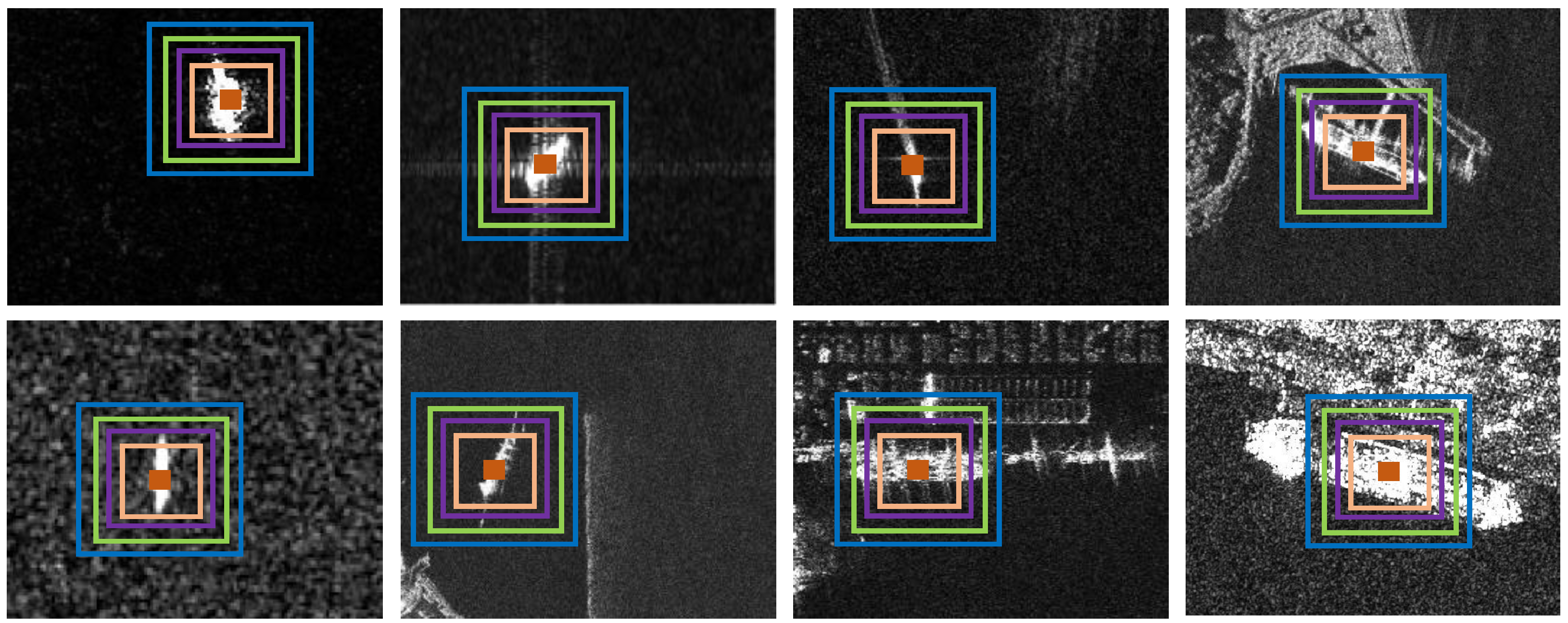
Ships in SAR images have various surroundings, as in Figure 2, e.g., river courses, islands, inshore facilities, harbors, and wakes. Moreover, because of the special imaging mechanisms of SAR, ships are also accompanied with cross-shape sidelobes, speckle noise, and granular pixel distribution [50]. These various surroundings pose differential effects to ship instance segmentation. It is very necessary to take them into consideration for better background discrimination ability in box prediction. Therefore, we design a global context information modeling block (GCIM-Block) to model global background context information, which can capture the spatial long-range dependences of ships to decrease false alarms and missed detections. GCIM-Block offers three main design concepts, i.e., (1) content-aware feature reassembly (CAFR), (2) multi receptive-field feature response (MRFFR), and (3) global feature self-attention (GFSA). Its workflow is shown in Figure 3. The input is $F_{\mathrm{ROI}}$ and the output is $F_{\mathrm{GCIM}-\mathrm{Block}}$.

2.1.1. Content-Aware Feature Reassembly (CAFR)

The standard ROI pooling size of the box prediction is $7\times 7$ while that of the mask prediction is $14\times 14$ [47]. Therefore, to maintain feature consistency between box and mask, before the global context modeling, we propose CAFR to up-sample the raw box feature maps from $7\times 7$ to $14\times 14$, which can also offer better modeling benefits in a larger feature space. We observe that this practice can offer a notable accuracy gain although the speed is sacrificed (see Section 5.1). Note that we abandon the common nearest neighbor or bilinear interpolation to reach this goal because they merely consider sub-pixel neighborhood, failing to capture the rich global context semantic information required by the dense prediction task. We also do not use the deconvolution because it applies the same kernel across the entire space, without considering the underlying global context content, limited by a limited field of view.

Differently, our proposed CAFR can enable the instance-specific content-aware handling while considering global context information, resulting in adaptive up-sampling kernels. Such a content-aware paradigm is also suggested by Wang et al. [51]. Figure 4 shows the implementation of CAFR. CAFR contains two processes—(i) content-aware kernel prediction and (ii) feature reassembly operation.

The former is used to encode contents so as to predict the up-sampling kernel K. The input is the ROI’s pooled feature maps denoted by $F_{\mathrm{ROI}}$. To reduce the computational burden, we first adopt a $1\times 1$ conv for channel compression where the compression is set to 0.5, i.e., from the raw 256 to the current 128, in consideration of the accuracy-speed trade-off. Then, a $3\times 3$ conv is used to encode the entire content whose kernel number is $2^2\times n^2$. Here, 2 denotes the up-sampling ratio, and n denotes the interpolation neighborhood scope to be considered, which is set to 5 empirically. In order to achieve the up-sampling kernel K across the entire $14\times 14$ feature space, the previous encoded content feature maps are shuffled in space, leading to the tensor with a $14\times 14\times n^2$ dimension.

Finally, it is normalized via a softmax calculation function defined by $e^{x_i}/{{\displaystyle \sum }}_j{e}^{x_j}$, leading to the final up-sampling kernel K. The $1\times 1\times n^2$ tensor alongside the depth direction represents the corresponding kernel for a single up-sampling operation from the raw location $l\left(i,j\right)$ to the required location $l^{\prime }\left(i^{\prime },j^{\prime }\right)$. Briefly, the above is described by

$$K=\mathrm{softmax}\left\{\mathrm{shuffle}\left[{\mathrm{conv}}_{3\times 3}\left({\mathrm{conv}}_{1\times 1}\left(F_{\mathrm{ROI}}\right)\right)\right]\right\}$$

(1)

The latter is to implement the feature reassembly, i.e., a convolution operation between the $n\times n$ neighbors of the location l denoted by $N\left(l, n\right)$ and the predicted kernel $K_{l^{\prime }}\in K$ corresponding to the required location l’. The above is described by

$$F_{\mathrm{ROI}}^{\prime }={\displaystyle \bigcup }_{l\in F_{\mathrm{ROI}}, l^{\prime }\in F_{\mathrm{ROI}}^{\prime }}N\left(l,n\right)\otimes K_{l^{\prime }}$$

(2)

where $F_{\mathrm{ROI}}^{\prime }$ denotes the output feature maps of CAFR, and $\otimes$ denotes the convolution operator.

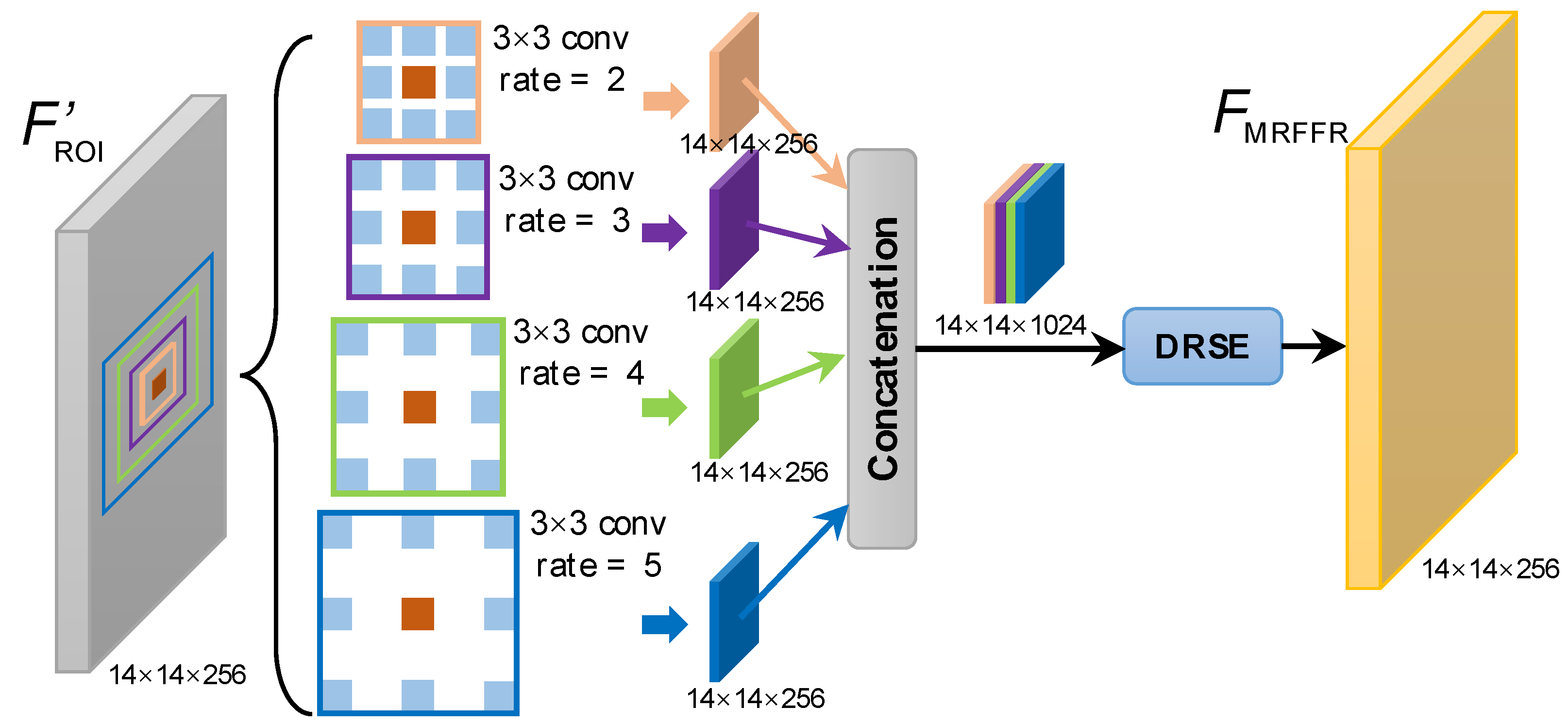
2.1.2. Multi Receptive-Field Feature Response (MRFFR)

Inspired by the idea of the multi resolution analysis (MRA) [52] widely used in the wavelet transform community, we propose MRFFR to analyze ships in resolution from fine to coarse, which can improve the richness of global context information, i.e., from single-scale context to multi-scale contexts. Specifically, we adopt multi dilated convolutions [53] with different dilated rates r to reach this aim as shown in Figure 5, where different scale or color boxes represent different context scopes. MRFFR can not only excite feature multi-resolution responses but also capture multi-scope context information, conducive to better global context modeling.

Figure 6 depicts the implementation of MRFFR. We adopt four $3\times 3$ convs with different dilated rates to trigger different resolution responses. More might bring better accuracy but will reduce speed. Then, the achieved four results are concatenated directly. Finally, we propose a dimension reduction squeeze-and-excitation (DRSE) to balance the contributions of different scope contexts and to achieve the channel reduction convenient for the subsequent processing. DRSE can model channel correlation to suppress useless channels and highlight valuable ones while reducing channel dimension, which reduces the risk of the training oscillation due to excessive irrelevant contextual backgrounds. We observe that only moderate contexts can enable better box and mask prediction.

The above is described by

$$F_{\mathrm{MRFFR}}=f_{\mathrm{DRSE}}\left\{\left[f_{3\times 3}^2\left(F_{\mathrm{ROI}}^{\prime }\right),f_{3\times 3}^3\left(F_{\mathrm{ROI}}^{\prime }\right),f_{3\times 3}^4\left(F_{\mathrm{ROI}}^{\prime }\right),f_{3\times 3}^5\left(F_{\mathrm{ROI}}^{\prime }\right)\right]\right\}$$

(3)

where $F_{\mathrm{ROI}}^{\prime }$ denotes the input, $F_{\mathrm{MRFFR}}$ denotes the output, $f_{3\times 3}^r$ denotes a $3\times 3$ conv with a dilated rate r, and $f_{\mathrm{DRSE}}$ denotes the DRSE operation to reduce channels from 1024 to 256.

Figure 7 depicts the implementation of DRSE. The input is denoted by X and output is denoted by Y. In the collateral branch, a global average pooling is used to achieve global spatial information, a $1\times 1$ conv and a sigmoid activation function are used to squeeze channels to highlight important ones. The squeeze ratio $p$ is set to 4 ($1024\to 256$). In the main branch, the input channel number is reduced directly by a $1\times 1$ conv and a ReLU activation. The broadcast element-wise multiplication is used for compressed channel weighting. In this way, DRSE models the channel correlation of input feature maps in a reduced dimension space. It uses the learned weights from the reduced dimension space to pay attention to the important features of the main branch. It avoids the potential information loss of the rude dimension reduction. In short, the above is described by

$$Y=\mathrm{ReLU}\left({\mathrm{conv}}_{1\times 1}\left(X\right)\right)\odot \sigma \left({\mathrm{conv}}_{1\times 1}\left(GAP\left(X\right)\right)\right)$$

(4)

where $\sigma$ denotes the sigmoid function and $\odot$ denotes the broadcast element-wise multiplication.

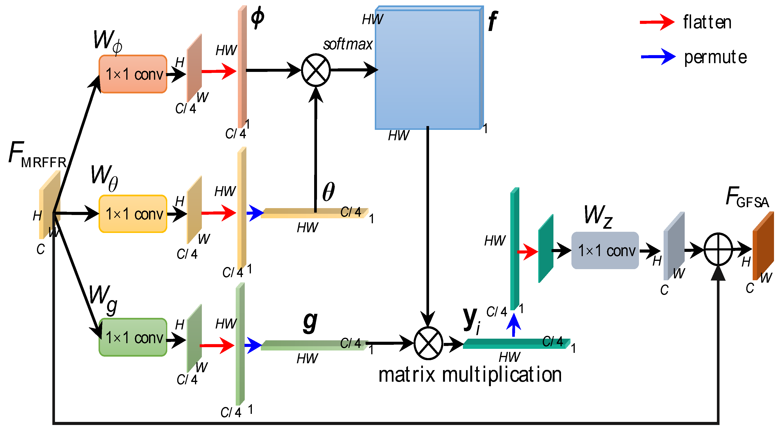
2.1.3. Global Feature Self-Attention (GFSA)

GFSA follows the basic idea of the non-local neural networks [54] to achieve the global context feature self-attention. It can be described by

$$y_i=\frac{1}{\zeta \left(x\right)}{{\displaystyle \sum }}_{\forall j}f\left(x_i,x_j\right)g\left(x_j\right)$$

(5)

where x denotes the input, i and j are the index position in the inputted feature maps across the whole H × W space. f is a pairwise function used to represent the spatial correlation between i and j. g is a unary function used to represent the inputted feature maps at position j. To a given i, j will enumerate the whole H × W space, resulting a sequence of spatial correlation between i and every position in the inputted feature maps. Through ${\displaystyle \sum }_{\forall j}f\times \mathrm{c}$, the i-position’s output $y_i$ is related with the entire space. This means that global long-range spatial dependencies are captured. Finally, $\zeta \left(x\right)$ is used to normalize the response.

We instantiate Equation (5) in Figure 8. Notably, Equation (5) is only to illustrate the process of calculating a single feature vector at the j-position ($y_i$) and the essence of achieving the global context feature self-attention. However, in the instantiation, the feature vectors at every position ($y$) are computed in parallel through matrix calculation in consideration of computational efficiency, and we need to use existing operators such as convolution and softmax to achieve the global context feature self-attention for simplicity. Specifically, in Figure 8, features at the i-position are denoted by $\varphi$ using a $1\times 1$ conv $W_{\varphi }$. Features at the j-position are denoted by $\theta$ using a $1\times 1$ conv $W_{\theta }$. We model unary function g as a linear embedding which is instantiated through a $1\times 1$ conv $W_g$, and embed features into $C/4$ channel space to reduce computational burdens. Moreover, pairwise function f is modeled as the Gaussian function $e^{x_i^T{x}_j}$ and normalization factor $\zeta \left(x\right)$ is modeled as ${\displaystyle \sum }_{\forall j}{e}^{x_i^T{x}_j}$. Therefore, we can instantiate f and the normalization process together through a softmax calculation function along the dimension j. Since $W_{\varphi }$ and $W_{\theta }$. are learnable, the spatial correlation f is obtained from adaptive learning between $\varphi$ and $\theta$. Note that in the global self-attention process, the sizes of features need to be transposed or shift between three dimension and two dimension, which is implemented through the permute and flatten operations, respectively. The response at the i-position $y_i$ is obtained by a matrix multiplication.

Since we embed features into $C/4$ channel space to reduce computational burdens before the global self-attention process, we need to recover the channel of features after the attention process through a $1\times 1$ conv $W_z$ for the adding operation.

Finally, we achieve the final global feature self-attention output $F_{\mathrm{GFSA}}$ that will be transmitted to the subsequent boundary-aware box prediction. Here, $F_{\mathrm{GFSA}}$ denotes the final output of GCIM-Block $F_{\mathrm{GCIM}-\mathrm{Block}}$.

2.2. Boundary-Aware Box Prediction Block (BABP-Block)

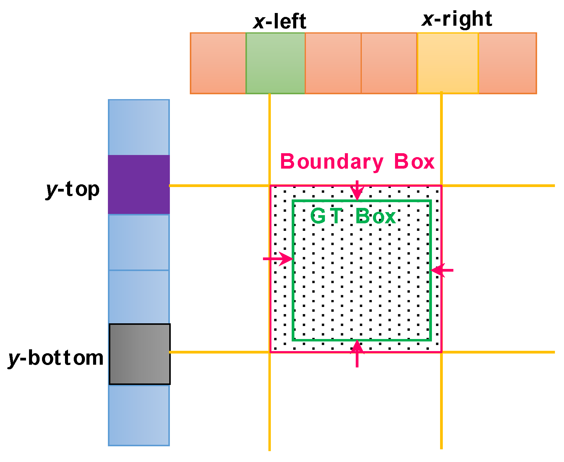
The traditional box prediction is implemented via estimating the bounding box’s center offset $\left(\Delta x,\Delta y\right)$ and the corresponding width and height offset $\left(\Delta w,\Delta h\right)$ with its ground truth (GT) to optimize network parameters, as shown in Figure 9a. Yet, this paradigm is not very suitable for SAR ships from the following two aspects.

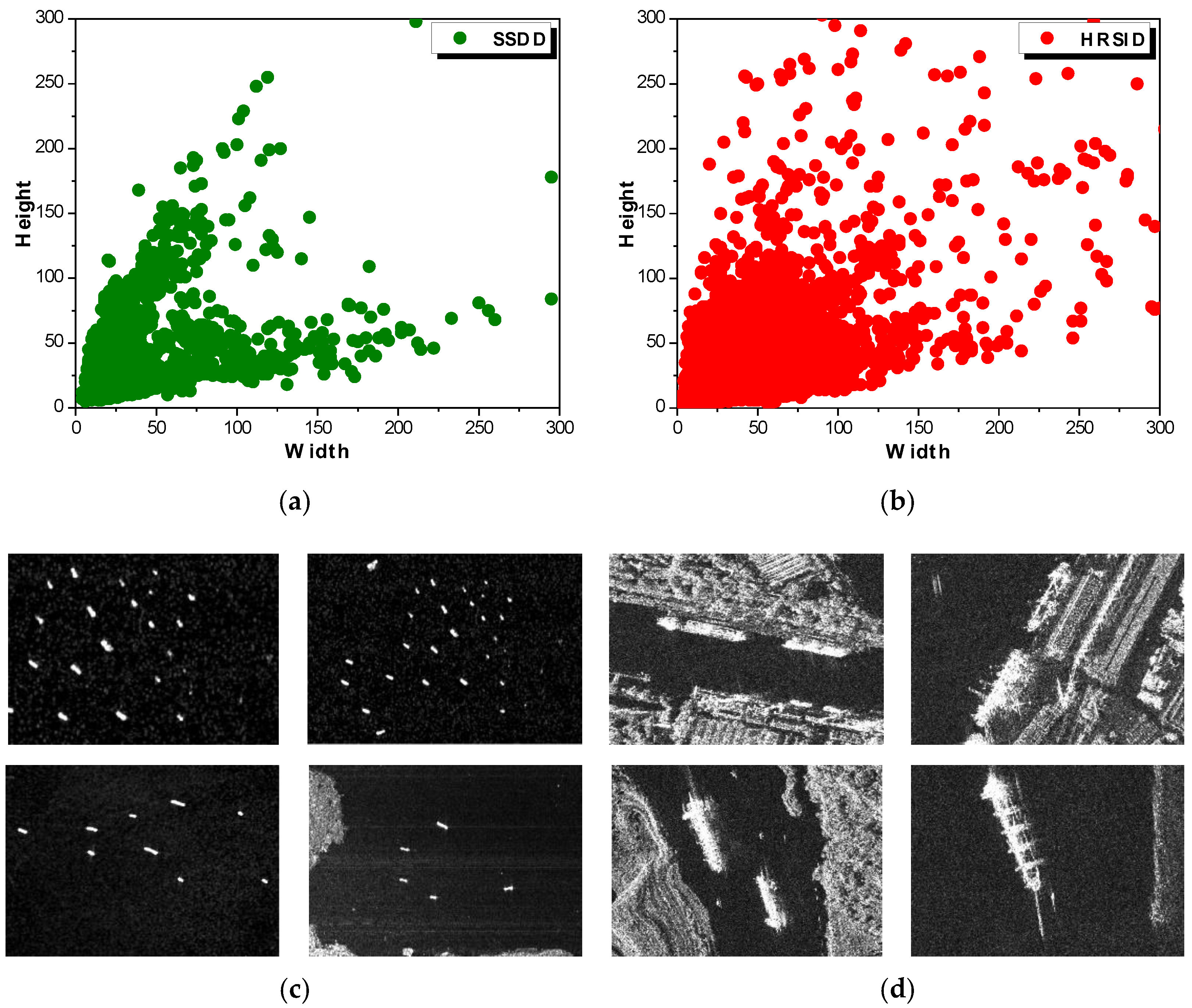
On the one side; as shown in Figure 10; SAR ships often exhibit a huge scale-difference due to a huge resolution difference; e.g.; 1m resolution for TerraSAR-X [55] and 20m resolution for Sentinel-1 [56]. This situation is called the cross-scale effect [39], e.g., the extremely small ships in Figure 10c vs. the extremely larger ships in Figure 10d. For example, the smallest ship in SSDD has only 28 pixels while the largest one has 62,878 pixels [57], where the scale ratio reaches 62,878/28 = 2245. For commonly-used two-stage models, presetting a series of prior anchors is required for RPN. Yet, no matter how the prior anchors are set; it is still difficult to cover such a dataset with a large scale-difference. In the dataset; since the proportion of small ships is higher than large ships; the size of the prior anchor is always closer to the small ship; but there will be a long space distance from the large ship. This will lead to the adjustment for the large ship anchors, as it becomes rather difficult if adopting the traditional scheme shown in Figure 9a. This is because it is time-consuming to adjust a small anchor to a large GT box; resulting in a great burden to the network training. As a result; the positioning accuracy of large ships will become poor

On the other side, it is rather challenging to locate the center of an SAR ship. Generally, different parts of the ship’s hull have different materials, resulting in differential radar electromagnetic scatterings (i.e., radar cross section, RCS [58]). This makes the pixel brightness distribution of the ship in one SAR image extremely uneven. In many cases, the strong scattering points of the ship are not in the geometric center of the hull, but in the bow or stern. This phenomenon may directly lead to the failure

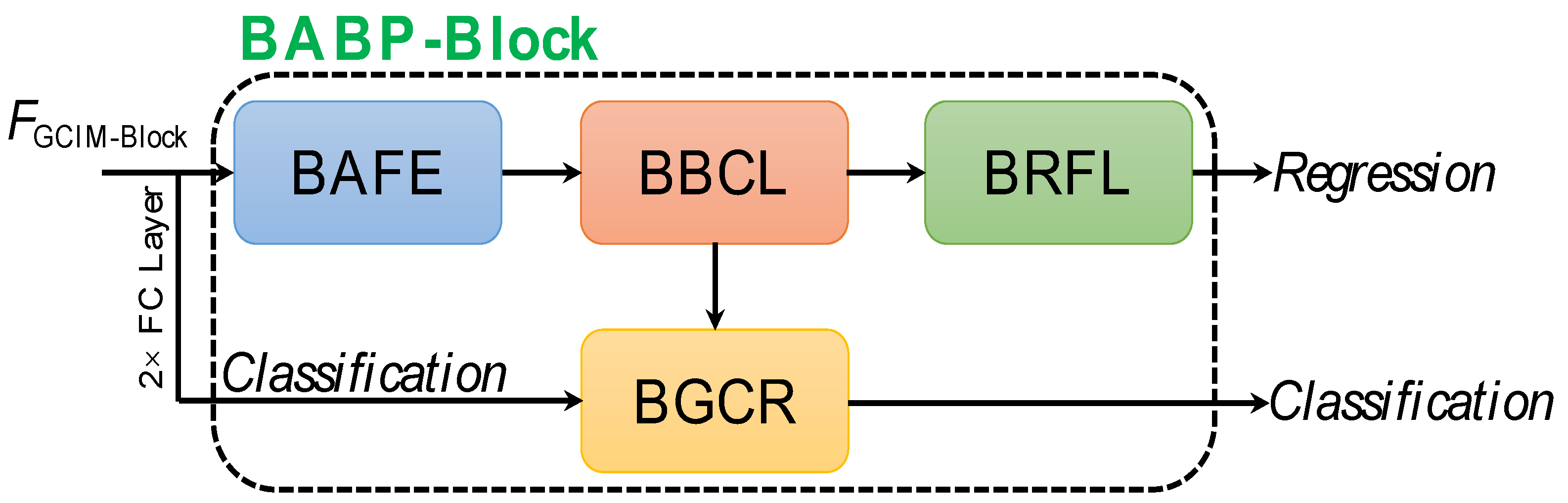
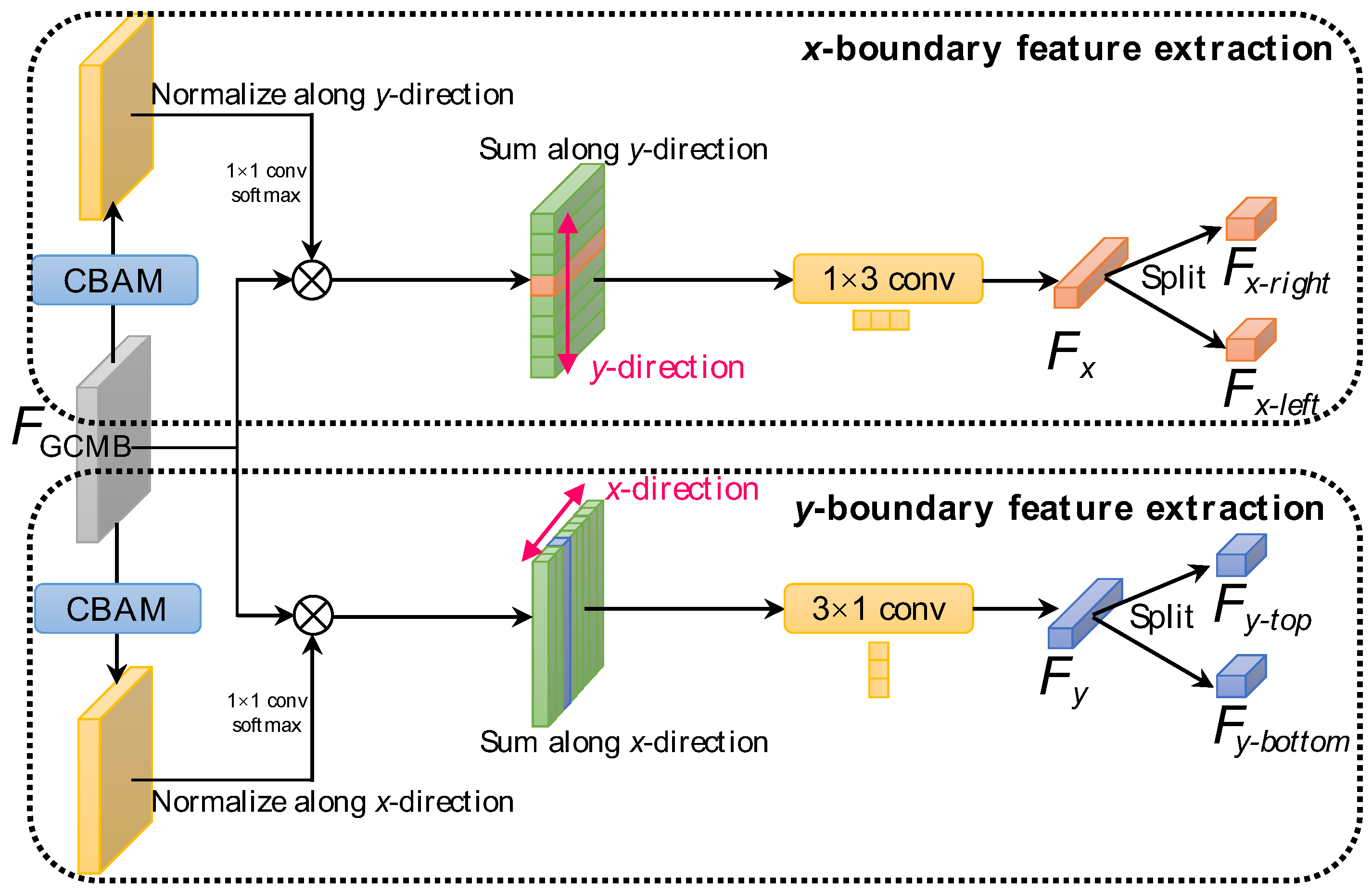
As shown above, we abandon the traditional scheme in Figure 9a, and adopt the boundary learning scheme in Figure 9b to implement the box prediction. We design a boundary-aware box prediction block (BABP-Block) to reach this goal, inspired by the gird idea from Wang et al. [59] and Lu et al. [60]. From Figure 9b, BABP-Block consists of two basic steps. (i) The first is to predict the coarse boundary of a ship marked by yellow dotted lines in the x-left, x-right, y-top and y-down (i.e., four yellow activate grids). (ii) The second is to adjust the box finely from the boundary box to the GT box. This stage is the same as the traditional scheme, but obviously it is much easier to adjust the resulting coarse boundary box to the GT box so as to achieve the final finer box. This is because the distance to be adjusted is greatly reduced. Such from coarse to fine prediction scheme divides the task into two stages where each stage is responsible for its own task, resulting in the dual-supervision of training, enabling better box prediction. Once the box prediction becomes more accurate, the mask prediction will become more accurate as well. BABP-Block offers four main design concepts, i.e., (1) boundary-aware feature extraction (BAFE), (2) boundary bucketing coarse localization (BBCL), (3) boundary regression fine localization (BRFL), and (4) boundary-guided classification rescoring (BGCR). Its workflow is depicted in Figure 11. The input is the feature maps of GCIM-Block’s output $F_{\mathrm{GCIM}-\mathrm{Block}}$.

2.2.1. Boundary-Aware Feature Extraction (BAFF)

The traditional feature extraction is implemented across the entire 2D space without distinguishing direction, i.e., four boundary directions including the x-left, x-right, y-top, and y-down. As a result, important boundary-sensitive features are not extracted. Thus, BAFF is arranged to solve this problem so as to ensure the subsequent boundary localization accuracy.

Figure 12 shows the implementation of BAFE. BAFE contains two parallel branches, i.e., x-boundary feature extraction and y-boundary feature extraction. Here, we take the x-boundary feature extraction as an example to introduce details. The same can be reasoned for the y-boundary feature extraction. First, we use a convolutional block attention module (CBAM) [61] to better capture direction-specific information of the ROI region. Then, a $1\times 1$ conv with a softmax activation is used to normalize the attention map which will be weighted to the raw feature maps by the matrix element-wise multiplication. Afterwards, we sum features along the y-direction and use a $1\times 3$ asymmetric conv to achieve the features along x-direction $F_x$. The above can be described by

$$F_x={{\displaystyle \sum }}_y{F}_{\mathrm{GCIM}-\mathrm{Block}}\left(y,:\right)\ast M_x\left(y,:\right)$$

(6)

where $M_x$ denotes the attention map of the x-boundary. Finally, $F_x$ is split into two subsets evenly, i.e., $F_{x-right}$ and $F_{x-left}$, to represent the features of the right and left boundaries.

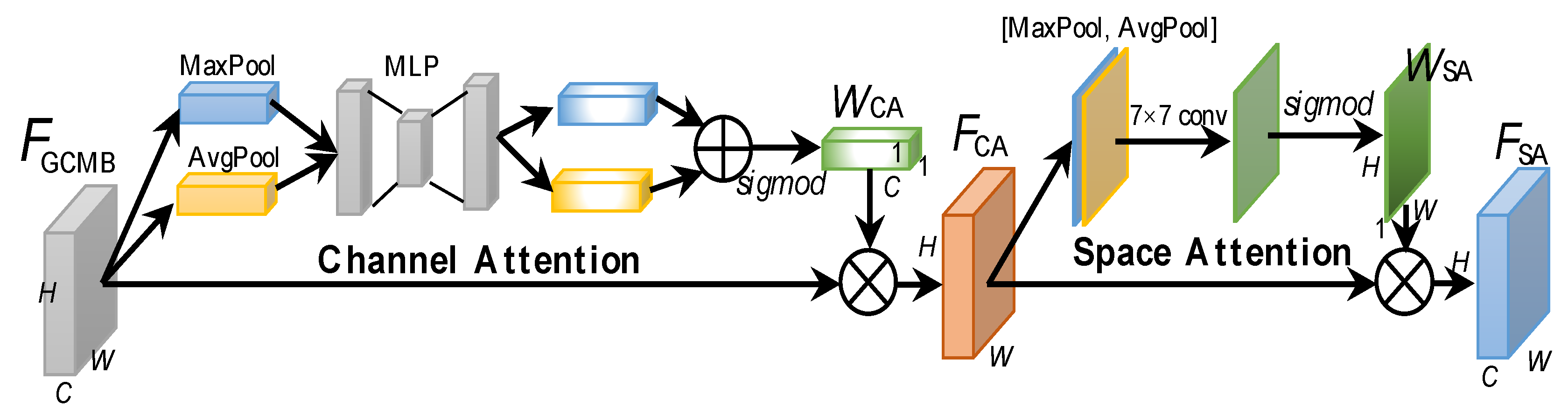
Figure 13 shows the implementation of CBAM. Let its input be $F_{\mathrm{GCIM}-\mathrm{Block}}\in {ℝ}^{H\times W\times C}$ where H and W are the height and width of feature maps and C is the channel number, then the channel attention is responsible for generating a channel-dimension weight matrix $W_{CA}\in {ℝ}^{1\times 1\times C}$ to measure the important levels of C channels; the space attention is responsible for generating a space-dimension weight matrix $W_{SA}\in {ℝ}^{H\times W\times 1}$ to measure the important levels of space-elements across the entire $H\times W$ space. They both range from 0 to 1 by a sigmoid activation which can enrich nonlinearity of neural networks for better performance, suggested by [61]. The result of the channel attention is denoted by $F_{CA}=F\times W_{CA}$. The result of the space attention is denoted by $F_{SA}=F_{CA}\times W_{SA}$. It should be noted that here, the space attention is executed following the channel attention. It is also feasible to change their order.

For the channel attention, a max-pooling (MaxPool) is used to capture its local response, and an average-pooling (AvgPool) is used to capture its global response. A multi-layer perceptron (MLP) is used to refine them for better fusion between the local and global responses. Finally, the results are normalized by a sigmoid function to obtain $W_{CA}$. The above is described by

$$W_{CA}=\sigma \left\{\mathrm{MLP}\left[\mathrm{MaxPool}\left(F\right)\right]+\mathrm{MLP}\left[\mathrm{AvgPool}\left(F\right)\right]\right\}$$

(7)

where $\sigma$ denotes the sigmoid activation defined by $1/\left(1+e^{-x}\right)$.

For the space attention, MaxPool and AvgPool are also used. Still, differently, they both operate on the channel dimension to achieve 2D feature maps. Their results are concatenated directly and convolved by a common conv layer, producing the 2D spatial attention map. Finally, the results are normalized by a sigmoid activation to obtain $W_{SA}$. The above is described by

$$W_{SA}=\sigma \{f_{7\times 7}\left([\mathrm{MaxPool}\left(F_{CA}\right),\mathrm{AvgPool}\left(F_{CA}\right)\right])\}$$

(8)

where $f^{7\times 7}$ is a $7\times 7$ conv recommended by their original report [61].

2.2.2. Boundary Bucketing Coarse Localization (BBCL)

After boundary-sensitive features are achieved by the previous BAFE stage, we follow the bucketing idea [62] to predict the box boundary, referred to as BBCL. The specific implementation scheme is consistent with Wang et al. [59]. This scheme divides the target space into multiple buckets, or called discrete grid cells [60]. This coarse boundary localization is completed by searching for the correct bucket, i.e., the one in which the boundary resides. Figure 14 shows the implementation of BBCL. The candidate regions are divided into 2k buckets on both x-direction and y-direction, with k buckets corresponding to each boundary. Here, k is equal to 14, because the feature map’s size is $14\times 14$. From Figure 14, we adopt a fully-connected (FC) layer to serve as a binary classifier to predict whether the boundary is located in or is the closest to the bucket on each side, based on the ship boundary-aware features $F_{x-right}$, $F_{x-left}$, $F_{y-right}$, and $F_{y-left}$. We achieve the boundary probabilities of four sides, denoted by $s_{x-right}$, $s_{x-left}$, $s_{y-right}$, and $s_{y-left}$. It should be noted that the boundary probabilities of four sides, i.e., $s_{x-right}$, $s_{x-left}$,$s_{y-right}$, and $s_{y-left}$ will be utilized for the final boundary-guided classification rescoring, which will be introduced in the next sections. Afterwards, the maximum activation value is then projected into the raw feature maps to achieve the corresponding index value. Finally, the four boundary positions are obtained, i.e., x-right, x-left, y-right, and y-left. In this way, the coarse boundary of a ship is predicted successfully.

2.2.3. Boundary Regression Fine Localization (BRFL)

After the coarse boundary of a ship is obtained, we need to finely adjust the box close to the GT box in order to eliminate the boundary effects of buckets, as shown in Figure 15. This process is the same as the traditional bounding box regression scheme. Specifically, we adopt a 4-way FC layer to complete this task, i.e., the center point correction and width-height adjustment. Since this process is operated in the predicted boundary box, the distance between the initial box and the GT box becomes smaller. Consequently, such a regression task will become more relaxing to deal with the cross-scale effect, because the positioning difficulty is shared by the previous boundary prediction stage.

Up to this point, we have achieved bounding box regression results by the regression branch in Figure 11.

2.2.4. Boundary-Guided Classification Rescoring (BGCR)

BBCL offers the localization reliability of the predicted boundary box, that is, the boundary probabilities of four sides $s_{x-right}$, $s_{x-left}$,$s_{y-right}$, and $s_{y-left}$ as previously introduced. The idea of rescoring is also shown in FCOS [63] where the final classification score is computed by using the predicted center-ness score and the raw classification score together. And it is a direct intuition that it should be conducive to maintaining the optimum box with both high classification confidence and accurate localization if fully leveraging them. Thus, we arrange a boundary-guided classification rescoring (BGCR) strategy to reach this aim, which is described by

$$s^{\text{'}}=\alpha ·s+\beta ·\frac{1}{4}\left(s_{x-right}+s_{x-left}+s_{y-right}+s_{y-left}\right)$$

(9)

where s denotes the original confidence score of the classification network (i.e., two FC layers in Figure 11), $s^{\text{'}}$ denotes the final confidence score, $\alpha$ denotes the weight coefficient of the original confidence score and $\beta$ denotes the weight coefficient of the localization reliability. In our work, $\alpha$ and $\beta$ are both set to 0.5 considering the trade-off between the spatial localization reliability and the classification reliability [64,65]. Here, in terms of the total localization reliability, we directly average the four sides’ boundary probabilities, because they seem to be equally important. Finally, the resulting score $s^{\prime }$ will be inputted to the non-maximum suppression (NMS) algorithm [48] to remove repeated detections.

3. Experiments

3.1. Dataset

Two public datasets SSDD [33] and HRSID [34] are used in our work. SSDD is available online at https://github.com/TianwenZhang0825/Official-SSDD (accessed on 1 March 2022). HRSID is available online at https://github.com/chaozhong2010/HRSID, accessed on 1 April 2022. SSDD offers 1160 samples collected from RadarSat-2, TerraSAR-X, and Sentinel-1. Polarizations are HH, VV, VH, and HV. Resolutions are from 1 m to 10 m. The test set has 232 samples with the filename suffix of 1 and 9. The remaining samples constitute the training set. HRSID offers 5604 samples collected from Sentinel-1 and TerraSAR-X. Polarizations are HH, HV, and VV. Resolutions are 0.5 m, 1 m and 3 m. The training set has 3642 samples and the test set has 1962.

3.2. Training Details

ResNet-101 [46] serves as the backbone network that is pretrained on ImageNet [66]. The FPN structure [40] is used to ensure multi-scale performance. We adopt the stochastic gradient descent (SGD) algorithm to train GCBANet and other nine comparison models by 12 epochs. The learning rate is 0.002 that is reduced by 10 times at 8-epoch and 11-epoch. The momentum is 0.9 and the weight decay is 0.0001. The batch size is 1 due to limited GPU memory. The training loss function and other hyper-parameters are same as the hybrid task cascade model [44]. The referenced source code we used for performance comparison is from MMDetection at https://github.com/open-mmlab/mmdetection (accessed on 1 March 2022).

3.3. Evaluation Criteria

The COCO metrics [67] are adopted. Its core index is the average precision ($AP$), i.e., the average value of precisions under ten intersection over union (IOU) thresholds from 0.50 to 0.95 with an interval of 0.05. $A{P}_{50}$ denotes the $AP$ of an IOU threshold of 0.50.$A{P}_{75}$ denotes $AP$ of an IOU threshold of 0.75. $A{P}_S$ denotes $AP$ of small ships (<322 pixels). $A{P}_M$ denotes the $AP$ of medium ships (>322 pixels and <962 pixels). $A{P}_L$ denotes the $AP$ of large ships (>962 pixels). Specifically, the IOU of the predicted mask and the ground truth mask is described by

$$IOU=\frac{P_{mask}\cap G_{mask}}{P_{mask}\cup G_{mask}}$$

(10)

where $P_{mask}$ represents the predicted mask and $G_{mask}$ represents the ground truth mask. According to a given IOU threshold and confidence threshold, the predictions of instance segmentation results can be divided into different categories, while true positive$\left(TP\right)$, false positive $\left(FP\right)$, and false negative$\left(FN\right)$ represent the number of samples in each category. Then, the corresponding precision value and recall value is described by

$$\mathrm{Precision}=\frac{TP}{TP+FP}$$

(11)

$$\mathrm{Recall}=\frac{TP}{TP+FN}$$

(12)

With confidence threshold changes, precision and recall will be different, with the result that the precision and recall curve $P\left(r\right)$ where the recall value serves as the abscissa and precision value serves as the ordinate in Cartesian coordinate system. Then, the $AP$ of a given IOU threshold is described by

$$A{P}_{IOU}={{\displaystyle \int }}_0^{1}P\left(r\right)dr$$

(13)

Then,$AP$ is the average value of 10 $A{P}_{IOU}$ whose IOU threshold ranges from 0.5 to 0.95 with the stride of 0.05., which is described by

$$AP=\frac{1}{10}\times {\displaystyle \sum }_{IOU=0.50}^{0.95}A{P}_{IOU}$$

(14)

4. Results

4.1. Quantitative Results

Table 1. Quantitative Results on SSDD. The suboptimal method is marked by underline “—”.

Method	Backbone	Box (%)						Mask (%)						FPS
		AP	AP50	AP75	APS	APM	APL	AP	AP50	AP75	APS	APM	APL
Mask R-CNN [47]	ResNet-101	62.0	91.5	75.4	62.0	64.4	19.7	57.8	88.5	72.1	57.2	60.8	27.4	11.05
Mask Scoring R-CNN [70]	ResNet-101	62.4	91.0	75.1	61.9	66.0	15.7	58.6	89.4	73.2	58.0	61.4	22.6	12.88
Cascade Mask R-CNN [43]	ResNet-101	63.0	89.6	75.2	62.4	66.0	12.0	56.6	87.5	70.5	56.3	58.8	22.6	10.55
PANet [71]	ResNet-101	63.3	93.4	75.4	63.4	65.5	40.8	59.6	91.1	74.0	59.3	61.0	52.1	13.65
YOLACT [68]	ResNet-101	54.0	90.6	61.2	56.9	48.2	12.6	48.4	88.0	52.1	47.3	53.5	40.2	15.47
GROIE [72]	ResNet-101	61.2	91.5	71.6	62.2	59.8	8.7	58.3	89.8	72.7	58.6	58.7	21.8	9.67
HQ-ISNet [35]	HRNetV2-W18	64.9	91.0	76.3	64.7	66.6	26.0	58.6	89.3	73.6	58.2	60.4	37.2	8.59
HQ-ISNet [35]	HRNetV2-W32	65.5	90.7	77.3	65.6	66.9	23.2	59.3	90.4	75.5	58.9	61.1	37.3	8.00
HQ-ISNet [35]	HRNetV2-W40	63.6	87.8	75.3	62.6	67.8	27.9	57.6	86.0	72.6	56.7	61.3	50.2	7.73
SA R-CNN [37]	ResNet-50-GCB	63.2	92.1	75.2	63.8	64.0	7.0	59.4	90.4	73.3	59.6	60.3	20.2	13.65
HTC [44]	ResNet-101	65.6	93.6	76.3	65.2	68.4	27.5	59.3	91.7	73.1	58.7	61.6	34.8	11.60
GCBANet (Ours)	ResNet-101	68.4	95.4	82.2	68.9	68.0	45.6	63.1	93.5	78.8	63.2	63.0	55.1	6.11
		+2.8	+1.8	+4.9	+3.3	+1.4	+4.8	+3.5	+1.8	+3.3	+3.6	+1.4	+3.0

and

Table 2. Quantitative results on HRSID. The suboptimal method is marked by Underline “—”.

Method	Backbone	Box (%)						Mask (%)						FPS
		AP	AP50	AP75	APS	APM	APL	AP	AP50	AP75	APS	APM	APL
Mask R-CNN [47]	ResNet-101	65.1	87.7	75.5	66.1	68.4	14.1	54.8	85.7	65.2	54.3	62.5	13.3	7.07
Mask Scoring R-CNN [70]	ResNet-101	65.2	87.6	75.4	66.5	67.4	13.4	54.9	85.1	65.9	54.5	61.5	12.9	8.24
Cascade Mask R-CNN [43]	ResNet-101	65.1	85.4	74.4	66.0	69.0	17.1	52.8	83.4	62.9	52.2	62.2	17.0	6.75
PANet [71]	ResNet-101	65.4	88.0	75.7	66.5	68.2	22.1	55.1	86.0	66.2	54.7	62.8	17.8	8.74
YOLACT [68]	ResNet-101	47.9	74.4	53.3	51.7	34.9	3.3	39.6	71.1	41.9	39.5	46.1	7.3	10.02
GROIE [72]	ResNet-101	65.4	87.8	75.5	66.5	67.2	21.8	55.4	85.8	66.9	54.9	63.5	19.7	6.19
HQ-ISNet [35]	HRNetV2-W18	66.0	86.1	75.6	67.1	66.3	8.9	53.4	84.2	64.3	53.2	59.7	10.7	5.50
HQ-ISNet [35]	HRNetV2-W32	66.7	86.9	76.3	67.8	68.3	16.8	54.6	85.0	65.8	54.2	61.7	13.4	5.12
HQ-ISNet [35]	HRNetV2-W40	66.7	86.2	76.3	67.9	68.6	11.7	54.2	84.3	64.9	53.9	61.9	12.8	4.95
SA R-CNN [37]	ResNet-50-GCB	65.2	88.3	75.2	66.4	65.4	10.2	55.2	86.2	66.7	54.9	60.9	12.3	8.74
HTC [44]	ResNet-101	66.6	86.0	77.1	67.6	69.0	28.1	55.2	84.9	66.5	54.7	63.8	19.2	7.42
GCBANet (Ours)	ResNet-101	69.4	89.8	79.2	70.4	71.3	32.2	57.3	88.6	68.9	57.0	64.3	25.9	4.06
		+2.7	+1.8	+2.1	+2.5	+2.3	+4.1	+1.9	+2.4	+2.0	+2.1	+0.5	+6.7

are the quantitative results on the SSDD and HRSID datasets. From Table 1 and Table 2, GCBANet achieves the best accuracy, that is, on SSDD, the box AP reaches 68.4% and the mask AP reaches 63.1%; on HRSIS, the box AP reaches 69.4% and the mask AP reaches 57.3%. The mask prediction has poorer indexes than the box prediction, because the pixel-level segmentation task is more difficult than the box-level detection task. GCBANet outperforms the other nine competitive models by a significant degree. On SSDD, it achieves 2.8% higher box AP and 3.5% higher mask AP than the previous most advanced model; on HRSID, they are 2.7% and 1.9%. This fully reveals the state-of-the-art performance of GCBANet. This accuracy advantage benefits from the combined action of the proposed GCIM-Block and BABP-Block. Certainly, the speed of GCBANet does not win advantages, compared with others, thereby the speed optimization is required in the future. Moreover, although YOLACT [68] offers the fastest detection speed because it is a one-stage model, its accuracy is too poor to satisfy application requirements.

Table 3. Computational complexity calculations of different methods. Here, we adopt the floating point of operations (FLOPs) to measure calculations whose unit is the giga multiply add calculations (GMACs) [69].

Method	Backbone	FLOPs (GMACs)
Mask R-CNN [47]	ResNet-101	121.32
Mask Scoring R-CNN [70]	ResNet-101	121.32
Cascade Mask R-CNN [43]	ResNet-101	226.31
PANet [71]	ResNet-101	127.66
YOLACT [68]	ResNet-101	67.14
GROIE [72]	ResNet-101	581.28
HQ-ISNet [35]	HRNetV2-W18	201.84
HQ-ISNet [35]	HRNetV2-W32	226.90
HQ-ISNet [35]	HRNetV2-W40	247.49
SA R-CNN [37]	ResNet-50-GCB	101.87
HTC [44]	ResNet-101	228.90
GCBANet (Ours)	ResNet-101	947.96

shows the computational complexity calculations of different methods. Here, we adopt the floating point of operations (FLOPs) to measure calculations whose unit is the giga multiply add calculations (GMACs) [69]. From Table 3, the calculation amount of GCBANet is more than the others, so future model computational complexity optimization is needed.

4.2. Qualitative Results

Figure 16 and Figure 17 are the quantitative results on SSDD and HRSID where we only show the quantitative comparison results with the second-best mask AP.

From Figure 16 and Figure 17, the following conclusions can be drawn:

• GCBANet can detect more ships, e.g., the #1 sample in Figure 16 and the #1 sample in Figure 17. This is because GCBANet can extract more salient features, leading to better box prediction.
• GCBANet can avoid many false alarms, e.g., the #3 sample in Figure 16 and the #4 sample in Figure 17. This is because the designed GCIM-Block can distinguish the foreground-background more effectively with the surrounding context information.
• GCBANet can enable ship instance segmentation with higher reliability. For example, for the same ship in the #2 sample in Figure 17, the confidence score of GROIE is 0.59, which is far smaller than that of our GCBANet 0.98. This advantage benefits from the boundary-guided classification rescoring strategy in the designed BABP-Block, which can consider both high classification confidence and accurate localization.
• GCBANet can locate large ships more accurately, e.g., the #4 sample in Figure 16 and the #2 sample in Figure 17. This advantage benefits from the designed BABP-Block, which can handle the cross-scale problem through the boundary prediction, so as to enable better box regression.

Given the above, GCBANet achieves state-of-the-art SAR ship instance segmentation performance.

5. Ablation Study

In this section, we will show the results of ablation studies to confirm the effectiveness of the proposed GCIM-Block and BABP-Block. Experiments are performed on SSDD.

5.1. Ablation Study on GCIM-Block

5.1.1. Effectiveness of GCIM-Block

Table 4. Quantitative Results with and Without GCIM-Block.

GCIM-Block	Box AP (%)	Mask AP (%)
	66.8	62.0
✓	68.4	63.1

shows the quantitative results with/without GCIM-Block. The GCIM-Block offers a 1.6% box AP gain and a 1.1% mask AP gain, showing its effectiveness. It can model the global background context information so as to capture spatial long-range dependences of ships, which can enable better background discrimination ability.

5.1.2. Component Analysis in GCIM-Block

We also make a component analysis in GCIM-Block, as shown in

Table 5. Quantitative Results Component Analysis in GCIM-Block.

CAFR 1	MRFFR 2	GFSA 3	Box AP (%)	Mask AP (%)	FPS
-	-	-	66.8	62.0	9.25
✓			67.5	62.4	7.86
✓	✓		68.4	62.8	6.72
✓	✓	✓	68.4	63.1	6.11

¹ CAFR denotes the content-aware feature reassembly. ² MRFFR denotes the multi receptive-field feature response. ³ GFSA denotes the global feature self-attention.

. From Table 5, each component can offer an observable accuracy improvement, either the box AP or the mask AP. This indicates that our well-designed idea is reasonable and our theoretical analysis in Section 2.1 is correct. Moreover, we observe that GFSA does not improve the box prediction performance, but it improves the mask prediction performance further. This is because the global feature self-attention is pixel-sensitive, which can enable better pixel classification capability.

5.2. Ablation Study on BABP-Block

5.2.1. Effectiveness of BABP-Block

Table 6. Quantitative Results with and Without BABP-Block.

BABP-Block	Box AP (%)	Mask AP (%)
	65.6	61.3
✓	68.4	63.1

shows the quantitative results with and without BABP-Block. BABP-Block offers a 2.8% box AP gain and a 1.8% mask AP gain, showing its effectiveness. It can offer better box prediction by predicting the boundary so as to enable better mask prediction. Thus, this boundary estimation scheme should be more suitable for SAR ships.

5.2.2. Component Analysis in BABP-Block

We also make a component analysis in BABP-Block as shown in

Table 7. Quantitative Results Component Analysis in BABP-Block.

BAFE 1	BBCL 2	BRFL 3	BGCR 4	Box AP (%)	Mask AP (%)	FPS
-	-	-	-	65.6	61.3	8.42
✓				66.0	61.9	7.36
✓	✓			66.7	62.2	6.58
✓	✓	✓		67.1	62.8	6.19
✓	✓	✓	✓	68.4	63.1	6.11

¹ BAFF denotes the boundary-aware feature extraction. ² BBCL denotes the boundary bucketing coarse localization. ³ BRFL denotes the boundary regression fine localization. ⁴ BGCR denotes the boundary-guided classification rescoring.

. From Table 7, each component is conducive to boosting accuracy, which shows their effectiveness. BAFE is able to extract more boundary-sensitive features so as to ensure accurate boundary bucketing coarse localization. BBCL locates four sides of the box to avoid long-distance regression, which boosts information flow. BRFL can enable more refined box regression. Finally, BGCR can leverage the boundary reliability to guide classification scores, so as to screen the detection results again, leading to more reliable predictions. As a result, the accuracy is improved progressively.

6. Conclusions

In this paper, GCBANet is proposed for better SAR ship instance segmentation. In GCBANet, GCIM-Block and BABP-Block are designed to ensure its excellent performance. Specifically, GCIM-Block is used to mitigate the inferences caused by the surroundings of ships and the mechanism of SAR imaging. BABP-Block is used to locate ships more precisely. Ablation studies can confirm the effectiveness of GCIM-Block and BABP-Block. The results on two open datasets reveal the state-of-the-art performance of GCBANet compared to the other nine competitive models. On SSDD, GCBANet achieves 2.8% higher box AP and 3.5% higher mask AP than the existing best model; on HRSID, they are 2.7% and 1.9%.

Our future work is as follows:

• We will consider optimizing the speed and the model computational complexity of GCBANet in the future.
• We will consider simplifying GCIM-Block to further reduce the computational cost in the future.

References

- Liu, C.; Zoughi, R. Adaptive Synthetic Aperture Radar (SAR) Imaging for Optimal Cross-Range Resolution and Image Quality in Nde Applications. IEEE Trans. Instrum. Meas. 2021, 70, 8005107. [Google Scholar] [CrossRef]
- Zhang, T.; Zhang, X.; Shi, J.; Wei, S. Hyperli-Net: A Hyper-Light Deep Learning Network for High-Accurate and High-Speed Ship Detection from Synthetic Aperture Radar Imagery. ISPRS J. Photogramm. Remote Sens. 2020, 167, 123–153. [Google Scholar] [CrossRef]
- Zhang, T.; Zhang, X. A Polarization Fusion Network with Geometric Feature Embedding for SAR Ship Classification. Pattern Recognit. 2021, 123, 108365. [Google Scholar] [CrossRef]
- Jarabo-Amores, P.; Rosa-Zurera, M.; Mata-Moya, D.D.L.; Vicen-Bueno, R.; Maldonado-Bascon, S. Spatial-Range Mean-Shift Filtering and Segmentation Applied to SAR Images. IEEE Trans. Instrum. Meas. 2011, 60, 584–597. [Google Scholar] [CrossRef]
- Gao, Y.; Qaseer, M.T.A.; Zoughi, R. Complex Permittivity Extraction from Synthetic Aperture Radar Images. IEEE Trans. Instrum. Meas. 2020, 69, 4919–4929. [Google Scholar] [CrossRef]
- Watanabe, T.; Yamada, H. Synthetic Aperture Imaging of near-Field Scatterers Mutually Coupled with an Antenna Array. IEEE Trans. Instrum. Meas. 2021, 70, 8001218. [Google Scholar] [CrossRef]
- Dudczyk, J.; Kawalec, A. Optimizing the minimum cost flow algorithm for the phase unwrapping process in SAR radar. Bull. Pol. Acad. Sci. Tech. 2014, 62, 511. [Google Scholar] [CrossRef] [Green Version]
- Ai, J.; Luo, Q.; Yang, X.; Yin, Z.; Xu, H. Outliers-Robust CFAR Detector of Gaussian Clutter Based on the Truncated-Maximum-Likelihood- Estimator in SAR Imagery. IEEE Trans. Intell. Transp. Syst. 2020, 21, 2039–2049. [Google Scholar] [CrossRef]
- Bentes, C.; Velotto, D.; Tings, B.O. Ship Classification in Terrasar-X Images with Convolutional Neural Networks. IEEE J. Oceanic. Eng. 2018, 43, 258–266. [Google Scholar] [CrossRef] [Green Version]
- Zhang, T.; Zhang, X.; Ke, X.; Liu, C.; Xu, X.; Zhan, X.; Wang, C.; Ahmad, I.; Zhou, Y.; Wei, S.; et al. Hog-ShipCLSNet: A Novel Deep Learning Network with Hog Feature Fusion for SAR Ship Classification. IEEE Trans. Geosci. Remote. Sens. 2021, 60, 5210322. [Google Scholar] [CrossRef]
- Koyama, C.N.; Gokon, H.; Jimbo, M.; Koshimura, S.; Sato, M. Disaster Debris Estimation Using High-Resolution Polarimetric Stereo-SAR. ISPRS J. Photogramm. Remote Sens. 2016, 120, 84–98. [Google Scholar] [CrossRef] [Green Version]
- Zhang, T.; Zhang, X. Squeeze-and-Excitation Laplacian Pyramid Network with Dual-Polarization Feature Fusion for Ship Classification in SAR Images. IEEE Geosci. Remote Sens. Lett. 2021, 19, 4019905. [Google Scholar] [CrossRef]
- Zhang, T.; Zhang, X.; Ke, X.; Zhan, X.; Shi, J.; Wei, S.; Pan, D.; Li, J.; Su, H.; Zhou, Y.; et al. Ls-Ssdd-V1.0: A Deep Learning Dataset Dedicated to Small Ship Detection from Large-Scale Sentinel-1 SAR Images. Remote Sens. 2020, 12, 2997. [Google Scholar] [CrossRef]
- Zeng, X.; Wei, S.; Shi, J.; Zhang, X. A Lightweight Adaptive Roi Extraction Network for Precise Aerial Image Instance Segmentation. IEEE Trans. Instrum. Meas. 2021, 70, 5018617. [Google Scholar] [CrossRef]
- Wang, B.; Dong, M.; Ren, M.; Wu, Z.; Guo, C.; Zhuang, T.; Pischler, O.; Xie, J. Automatic Fault Diagnosis of Infrared Insulator Images Based on Image Instance Segmentation and Temperature Analysis. IEEE Trans. Instrum. Meas. 2020, 69, 5345–5355. [Google Scholar] [CrossRef]
- Tu, B.; Liao, X.; Zhou, C.; Chen, S.; He, W. Feature Extraction Using Multitask Superpixel Auxiliary Learning for Hyperspectral Classification. IEEE Trans. Instrum. Meas. 2021, 70, 1–16. [Google Scholar] [CrossRef]
- Chen, S.W.; Cui, X.C.; Wang, X.S.; Xiao, S.P. Speckle-Free SAR Image Ship Detection. IEEE Trans. Image Process. 2021, 30, 5969–5983. [Google Scholar] [CrossRef]
- Zhang, T.; Zhang, X. A Full-Level Context Squeeze-and-Excitation Roi Extractor for SAR Ship Instance Segmentation. IEEE Geosci. Remote Sens. Lett. 2022. early access. [Google Scholar] [CrossRef]
- Cui, Z.; Li, Q.; Cao, Z.; Liu, N. Dense Attention Pyramid Networks for Multi-Scale Ship Detection in SAR Images. IEEE Trans. Geosci. Remote. Sens. 2019, 57, 8983–8997. [Google Scholar] [CrossRef]
- Zhang, T.; Zhang, X.; Liu, C.; Shi, J.; Wei, S.; Ahmad, I.; Su, H.; Zhan, X.; Zhou, Y.; Pan, D.; et al. Balance Learning for Ship Detection from Synthetic Aperture Radar Remote Sensing Imagery. ISPRS J. Photogramm. Remote Sens. 2021, 182, 190–207. [Google Scholar] [CrossRef]
- Sun, Z.; Dai, M.; Leng, X.; Lei, Y.; Xiong, B.; Ji, K.; Kuang, G. An Anchor-Free Detection Method for Ship Targets in High-Resolution SAR Images. IEEE J. Sel. Top. Appl. Earth Obs. Remote Sens. 2021, 14, 7799–7816. [Google Scholar] [CrossRef]
- Zhang, T.; Zhang, X.; Shi, J.; Wei, S. Depthwise Separable Convolution Neural Network for High-Speed SAR Ship Detection. Remote Sens. 2019, 11, 2483. [Google Scholar] [CrossRef] [Green Version]
- Zhang, T.; Zhang, X. Shipdenet-20: An Only 20 Convolution Layers and <1-Mb Lightweight SAR Ship Detector. IEEE Geosci. Remote Sens. Lett. 2021, 18, 1234–1238. [Google Scholar] [CrossRef]
- Song, J.; Kim, D.-J.; Kang, K.-M. Automated Procurement of Training Data for Machine Learning Algorithm on Ship Detection Using AIS Information. Remote Sens. 2020, 12, 1443. [Google Scholar] [CrossRef]
- Gao, G.; Shi, G. CFAR Ship Detection in Nonhomogeneous Sea Clutter Using Polarimetric SAR Data Based on the Notch Filter. IEEE Trans. Geosci. Remote. Sens. 2017, 55, 4811–4824. [Google Scholar] [CrossRef]
- Yang, H.; Cao, Z.; Cui, Z.; Pi, Y. Saliency Detection of Targets in Polarimetric SAR Images Based on Globally Weighted Perturbation Filters. ISPRS J. Photogramm. Remote Sens. 2019, 147, 65–79. [Google Scholar] [CrossRef]
- Wang, X.; Li, G.; Zhang, X.P.; He, Y. A Fast Cfar Algorithm Based on Density-Censoring Operation for Ship Detection in SAR Images. IEEE Signal Process. Lett. 2021, 28, 1085–1089. [Google Scholar] [CrossRef]
- LeCun, Y.; Bottou, L.; Bengio, Y.; Haffner, P. Gradient-based learning applied to document recognition. Proc. IEEE 1998, 86, 2278. [Google Scholar] [CrossRef] [Green Version]
- Krizhevsky, A.; Sutskever, I.; Hinton, G.E. Imagenet Classification with Deep Convolutional Neural Networks. In Proceedings of the International Conference on Neural Information Processing Systems (NIPS), Lake Tahoe, NV, USA, 3–8 December 2012; pp. 1097–1105. [Google Scholar]
- Simonyan, K.; Zisserman, A. Very Deep Convolutional Networks for Large-Scale Image Recognition. In Proceedings of the International Conference on Learning Representations (ICLR), San Diego, CA, USA, 7–9 May 2015; pp. 1–14. [Google Scholar]
- Girshick, R. Fast R-CNN. In Proceedings of the IEEE International Conference on Computer Vision, Santiago, Chile, 7–13 December 2015; p. 1440. [Google Scholar]
- Ren, S.; He, K.; Girshick, R.; Sun, J. Faster R-CNN: Towards Real-Time Object Detection with Region Proposal Networks. IEEE Trans. Pattern Anal. Mach. Intell. 2017, 39, 1137–1149. [Google Scholar] [CrossRef] [Green Version]
- Zhang, T.; Zhang, X.; Li, J.; Xu, X.; Wang, B.; Zhan, X.; Xu, Y.; Ke, X.; Zeng, T.; Su, H.; et al. SAR Ship Detection Dataset (SSDD): Official Release and Comprehensive Data Analysis. Remote Sens. 2021, 13, 3690. [Google Scholar] [CrossRef]
- Wei, S.; Zeng, X.; Qu, Q.; Wang, M.; Su, H.; Shi, J. HRSID: A High-Resolution SAR Images Dataset for Ship Detection and Instance Segmentation. IEEE Access. 2020, 8, 120234–120254. [Google Scholar] [CrossRef]
- Su, H.; Wei, S.; Liu, S.; Liang, J.; Wang, C.; Shi, J.; Zhang, X. HQ-ISNet: High-Quality Instance Segmentation for Remote Sensing Imagery. Remote Sens. 2020, 12, 989. [Google Scholar] [CrossRef] [Green Version]
- Gao, F.; Huo, Y.; Wang, J.; Hussain, A.; Zhou, H. Anchor-Free SAR Ship Instance Segmentation with Centroid-Distance Based Loss. IEEE J. Sel. Top. Appl. Earth Obs. Remote Sens. 2021, 14, 11352–11371. [Google Scholar] [CrossRef]
- Zhao, D.; Zhu, C.; Qi, J.; Qi, X.; Su, Z.; Shi, Z. Synergistic Attention for Ship Instance Segmentation in SAR Images. Remote Sens. 2021, 13, 4384. [Google Scholar] [CrossRef]
- Wang, J.; Chen, K.; Yang, S.; Loy, C.C.; Lin, D. Region Proposal by Guided Anchoring. In Proceedings of the IEEE Conference on Computer Vision and Pattern Recognition (CVPR), Long Beach, CA, USA, 16–20 June 2019; pp. 2960–2969. [Google Scholar]
- Zhou, Z.; Guan, R.; Cui, Z.; Cao, Z.; Pi, Y.; Yang, J. Scale Expansion Pyramid Network for Cross-Scale Object Detection in SAR Images. In Proceedings of the IEEE International Geoscience and Remote Sensing Symposium (IGARSS), Brussels, Belgium, 11–16 July 2021; pp. 5291–5294. [Google Scholar]
- Zhang, T.; Zhang, X.; Ke, X. Quad-FPN: A Novel Quad Feature Pyramid Network for SAR Ship Detection. Remote Sens. 2021, 13, 2771. [Google Scholar] [CrossRef]
- Li, J.; Qu, C.; Shao, J. Ship Detection in SAR Images Based on an Improved Faster R-CNN. In Proceedings of the SAR in Big Data Era: Models, Methods and Applications (BIGSARDATA), Beijing, China, 13–14 November 2017; pp. 1–6. [Google Scholar]
- Github. Available online: https://github.com/TianwenZhang0825/GCBANet (accessed on 1 March 2022).
- Cai, Z.; Vasconcelos, N. Cascade R-CNN: High Quality Object Detection and Instance Segmentation. IEEE Trans. Pattern Anal. Mach. Intell. 2021, 43, 1483–1498. [Google Scholar] [CrossRef] [PubMed] [Green Version]
- Chen, K.; Ouyang, W.; Loy, C.C.; Lin, D.; Pang, J.; Wang, J.; Xiong, L.; Li, X.; Sun, S.; Feng, W.; et al. Hybrid Task Cascade for Instance Segmentation. In Proceedings of the IEEE/CVF Conference on Computer Vision and Pattern Recognition (CVPR), Long Beach, CA, USA, 16–20 June 2019; pp. 4969–4978. [Google Scholar]
- Wang, J.; Sun, K.; Cheng, T.; Jiang, B.; Deng, C.; Zhao, Y.; Xiao, B.; Liu, D.; Mu, Y.; Tan, M.; et al. Deep High-Resolution Representation Learning for Visual Recognition. IEEE Trans. Pattern Anal. Mach. Intell. 2020, 43, 3349–3364. [Google Scholar] [CrossRef] [Green Version]
- He, K.; Zhang, X.; Ren, S.; Sun, J. Deep Residual Learning for Image Recognition. In Proceedings of the IEEE Conference on Computer Vision and Pattern Recognition (CVPR), Las Vegas, NV, USA, 26 June–1 July 2016; pp. 770–778. [Google Scholar]
- He, K.; Gkioxari, G.; Dollar, P.; Girshick, R. Mask R-CNN. In Proceedings of the IEEE International Conference on Computer Vision (ICCV), Venice, Italy, 22–29 October 2017; pp. 2980–2988. [Google Scholar]
- Hosang, J.; Benenson, R.; Schiele, B. Learning Non-Maximum Suppression. In Proceedings of the IEEE Conference on Computer Vision and Pattern Recognition (CVPR), Honolulu, HI, USA, 21–26 July 2017; pp. 6469–6477. [Google Scholar]
- Hafiz, A.M.; Bhat, G.M. A Survey on Instance Segmentation: State of the Art. Int. J. Multimed. Inf. Retr. 2020, 9, 171–189. [Google Scholar] [CrossRef]
- Zhang, T.; Zhang, X.; Shi, J.; Wei, S.; Wang, J.; Li, J.; Zhou, Y.; Su, H. Balance Scene Learning Mechanism for Offshore and Inshore Ship Detection in SAR Images. IEEE Geosci. Remote Sens. Lett. 2020, 19, 4004905. [Google Scholar] [CrossRef]
- Wang, J.; Chen, K.; Xu, R.; Liu, Z.; Loy, C.C.; Din, D. Carafe: Content-Aware Reassembly of Features. In Proceedings of the IEEE/CVF International Conference on Computer Vision (ICCV), Seoul, Korea, 27–28 October 2019; pp. 3007–3016. [Google Scholar]
- Benedetto, J.J.; Treiber, O.M. Wavelet Frames: Multiresolution Analysis and Extension Principles. In Wavelet Transforms and Time-Frequency Signal Analysis; Debnath, L., Ed.; Birkhäuser Boston: Boston, MA, USA, 2001; pp. 3–36. [Google Scholar]
- Yu, F.; Koltun, V. Multi-scale context aggregation by dilated convolutions. In Proceedings of the 4th International Conference on Learning Representations, San Juan, PR, USA, 2–4 May 2016; pp. 1–13. [Google Scholar]
- Wang, X.; Girshick, R.; Gupta, A.; He, K. Non-local neural networks. In Proceedings of the IEEE Conference on Computer Vision and Pattern Recognition, Salt Lake City, GA, USA, 18–22 June 2018; pp. 7794–7803. [Google Scholar]
- Buckreuss, S.; Schättler, B.; Fritz, T.; Mittermayer, J.; Kahle, R.; Maurer, E.; Böer, J.; Bachmann, M.; Mrowka, F.; Schwarz, E.; et al. Ten Years of TerraSAR-X Operations. Remote Sens. 2018, 10, 873. [Google Scholar] [CrossRef] [Green Version]
- Torres, R.; Snoeij, P.; Geudtner, D.; Bibby, D.; Davidson, M.; Attema, E.; Potin, P.; Brown, M.; Bruno, C.; Miranda, N.; et al. GMES Sentinel-1 Mission. Remote Sens. Environ. 2012, 120, 9–24. [Google Scholar] [CrossRef]
- Zhang, T.; Zhang, X. High-Speed Ship Detection in SAR Images Based on a Grid Convolutional Neural Network. Remote Sens. 2019, 11, 1206. [Google Scholar] [CrossRef] [Green Version]
- Iervolino, P.; Guida, R.; Whittaker, P. A Model for the Backscattering from a Canonical Ship in SAR Imagery. IEEE J. Sel. Top. Appl. Earth Obs. Remote Sens. 2016, 9, 1163–1175. [Google Scholar] [CrossRef] [Green Version]
- Wang, J.; Zhang, W.; Cao, Y.; Chen, K.; Pang, J.; Gong, T.; Lin, D.; Shi, J.; Loy, C.C. Side-Aware Boundary Localization for More Precise Object Detection. In Proceedings of the Computer Vision—ECCV 2020, 16th European Conference, Glasgow, UK, 23–28 August 2020; pp. 403–419. [Google Scholar]
- Lu, X.; Li, B.; Yue, Y.; Li, Q.; Yan, J. Grid R-CNN. In Proceedings of the IEEE/CVF Conference on Computer Vision and Pattern Recognition (CVPR), Long Beach, CA, USA, 16–20 June 2019; pp. 7355–7364. [Google Scholar]
- Woo, S.; Park, J.; Lee, J.-Y.; Kweon, I.S. Cbam: Convolutional Block Attention Module. In Proceedings of the European Conference on Computer Vision (ECCV), Munich, Germany, 8–14 September 2018; pp. 3–19. [Google Scholar]
- Tom, K.; Ondrej, B. Curriculum learning and minibatch bucketing in neural machine translation. arXiv 2017, arXiv:1707.09533. [Google Scholar]
- Tian, Z.; Shen, C.; Chen, H.; He, T. FCOS: Fully Convolutional One-Stage Object Detection. In Proceedings of the 2019 IEEE/CVF International Conference on Computer Vision (ICCV), Seoul, Korea, 27–28 October 2019; p. 9626. [Google Scholar]
- Rybak, Ł.; Dudczyk, J. Variant of Data Particle Geometrical Divide for Imbalanced Data Sets Classification by the Example of Occupancy Detection. Appl. Sci. 2021, 11, 4970. [Google Scholar] [CrossRef]
- Chen, H.; Zhang, F.; Tang, B.; Yin, Q.; Sun, X. Slim and Efficient Neural Network Design for Resource-Constrained SAR Target Recognition. Remote Sens. 2018, 10, 1618. [Google Scholar] [CrossRef] [Green Version]
- He, K.; Girshick, R.; Dollar, P. Rethinking Imagenet Pre-Training. In Proceedings of the IEEE International Conference on Computer Vision (ICCV), Seoul, Korea, 27–28 October 2019; pp. 4917–4926. [Google Scholar]
- Lin, T.-Y.; Maire, M.; Belongie, S.; Hays, J.; Perona, P.; Ramanan, D.; Zitnick, C.L.; Dollar, P. Microsoft Coco: Common Objects in Context. In Proceedings of the European Conference on Computer Vision (ECCV), 13th European Conference, Zurich, Switzerland, 6–12 September 2014; pp. 740–755. [Google Scholar]
- Bolya, D.; Zhou, C.; Xiao, F.; Lee, Y.J. Yolact: Real-Time Instance Segmentation. In Proceedings of the 2019 IEEE/CVF International Conference on Computer Vision (ICCV), Seoul, Korea, 27–28 October 2019; pp. 9156–9165. [Google Scholar]
- Eric, Q. Floating-Point Fused Multiply–Add Architectures. Ph.D. Thesis, The University of Texas at Austin, Austin, TX, USA, 2007. [Google Scholar]
- Huang, Z.; Huang, L.; Gong, Y.; Huang, C.; Wang, X. Mask Scoring R-CNN. In Proceedings of the 2019 IEEE/CVF Conference on Computer Vision and Pattern Recognition (CVPR), Long Beach, CA, USA, 16–20 June 2019; pp. 6402–6411. [Google Scholar]
- Liu, S.; Qi, L.; Qin, H.; Shi, J.; Jia, J. Path Aggregation Network for Instance Segmentation. In Proceedings of the IEEE Conference on Computer Vision and Pattern Recognition (CVPR), Salt Lake City, GA, USA, 18–22 June 2018; pp. 8759–8768. [Google Scholar]
- Rossi, L.; Karimi, A.; Prati, A. A Novel Region of Interest Extraction Layer for Instance Segmentation. In Proceedings of the International Conference on Pattern Recognition (ICPR), Milan, Italy, 10–15 January 2021; pp. 2203–2209. [Google Scholar]
Figure 1.
The architecture of the global context boundary-aware network (GCBANet). F denotes the feature maps of the backbone network. RPN denotes the region proposal network. FROI-i denotes the pooled ROI features in the i-th stage. Bi denotes the box prediction in the i-th stage. Mi denotes the mask prediction in the i-th stage. GCBANet adopts a cascade structure which sets three stages to refine box and mask prediction. GCIM-Block denotes the global context modeling block. BABP-Block denotes the boundary-aware box prediction block. NMS denotes non-maximum suppression.
Figure 2.
Various surroundings of ships in SAR images.
Figure 3.
Workflow of the global context information modeling block (GCIM-Block). Here, CAFR denotes the content-aware feature reassembly. MRFFR denotes the multi receptive-field feature response. GFSA denotes the global feature self-attention.
Figure 4.
Implementation of the content-aware feature reassembly (CAFR) in the GCIM-Block.
Figure 5.
Multi receptive-field feature response of SAR ships.
Figure 6.
Implementation of the multi receptive-field feature response (MRFFR) in GCIM-Block. DRSE denotes the dimension reduction squeeze-and-excitation.
Figure 7.
Implementation of dimension reduction squeeze-and-excitation (DRSE) in the MRFFR.
Figure 8.
Implementation of the global feature self-attention (GFSA) in GCIM-Block.
Figure 9.
Different box prediction forms. (a) The traditional bounding box’s center offset and the corresponding width and height offset estimation. (b) The bounding box’s boundary estimation of this paper, which contains two basic steps, i.e., boundary prediction and location fine regression. The red colored box denotes prediction box. The green colored box denotes ground truth box. The green colored dot denotes the center of ground truth box. The red colored arrow denotes the trend of bounding box regression.
Figure 10.
Some cross-scale SAR ships. (a) Ship size distribution in SSDD. (b) Ship size distribution in HRSID. (c) Small ships. (d) Large ships.
Figure 11.
Workflow of the boundary-aware box prediction block (BABP-Block). Here, BAFF denotes the boundary-aware feature extraction, BBCL denotes the boundary bucketing coarse localization, BRFL denotes the boundary regression refined localization and BGCR denotes the boundary-guided classification rescoring.
Figure 12.
Implementation of the boundary-aware feature extraction (BAFE) used in BABP-Block.
Figure 13.
Implementation of the convolutional block attention module (CBAM) used in BAFE.
Figure 14.
Implementation of the boundary bucketing coarse localization (BBCL) used in BABP-Block.
Figure 15.
Implementation of the boundary regression fine localization (BRFL) used in BABP-Block.
Figure 16.
Qualitative results on SSDD. (a) PANet with the second-best mask AP. (b) GCBANet. Green boxes denote the ground truths. Orange boxes denote the false alarms (i.e., false positives, FP). Red circles denote the missed detections (i.e., false negatives, FN). #i denote the ith picture of results.
Figure 17.
Qualitative results on HRSID. (a) GROIE with the second-best mask AP. (b) GCBANet. Green boxes denote the ground truths. Orange boxes denote the false alarms (i.e., false positives, FP). Red circles denote the missed detections (i.e., false negatives, FN). #i denote the ith picture of results.