Article

A Study on the Dynamic Effects and Ecological Stress of Eco-Environment in the Headwaters of the Yangtze River Based on Improved DeepLab V3+ Network

1
Institute of Geophysics & Geomatics, China University of Geosciences, Wuhan 430079, China
2
Land Satellite Remote Sensing Application Center, Ministry of Natural Resources of the People’s Republic of China, Beijing 100048, China
*
Author to whom correspondence should be addressed.
Submission received: 15 March 2022 / Revised: 3 May 2022 / Accepted: 4 May 2022 / Published: 6 May 2022

Abstract

:
The headwaters of the Yangtze River are a complicated system composed of different eco-environment elements. The abnormal moisture and energy exchanges between the atmosphere and earth systems caused by global climate change are predicted to produce drastic changes in these eco-environment elements. In order to study the dynamic effect and ecological stress in the eco-environment, we adapted the Double Attention Mechanism (DAM) to improve the performance of the DeepLab V3+ network in large-scale semantic segmentation. We proposed Elements Fragmentation (EF) and Elements Information Content (EIC) to quantitatively analyze the spatial distribution characteristics and spatial relationships of eco-environment elements. In this paper, the following conclusions were drawn: (1) we established sample sets based on “Sentinel-2” remote sensing images using the interpretation signs of eco-environment elements; (2) the mAP, mIoU, and Kappa of the improved DeepLab V3+ method were 0.639, 0.778, and 0.825, respectively, which demonstrates a good ability to distinguish the eco-environment elements; (3) between 2015 and 2021, EF gradually increased from 0.2234 to 0.2394, and EIC increased from 23.80 to 25.32, which shows that the eco-environment is oriented to complex, heterogeneous, and discontinuous processes; (4) the headwaters of the Yangtze River are a community of life, and thus we should build a multifunctional ecological management system with which to implement well-organized and efficient scientific ecological rehabilitation projects.

Graphical Abstract

1. Introduction

The headwaters of the Yangtze River are a complicated system composed of different eco-environment elements, including glaciers, lakes, grasslands, and bare land [1]. Over the past half-century, the glaciers in the headwaters of the Yangtze River have been shrinking [2,3]. Surface water is an important component of the cryosphere and the unique underlying surface of the plateau, and its abnormal circulation is directly threatening the ecological security of the headwaters of the Yangtze River and the basin as a whole [4,5,6]. Therefore, it is of great geoscientific and ecological significance to study the ecological stress and dynamic effects of eco-environment elements in the headwaters of the Yangtze River.
There is a series of studies on the relationship between glaciers and climate change, the influence of melting glaciers on runoff, and the control of grassland development [7,8]. With the growth of human needs and ecological requirements, the demand for normalization, intelligence, and elaboration in monitoring the eco-environment is increasing [9,10]. The introduction of remote sensing has expanded the horizons of eco-environment researches and improved our understanding of the region [11,12]. The research methods utilized to study the eco-environment in the headwaters of the Yangtze River mainly include the basin hydrological model, the climate model, and the landscape ecology model [13,14,15]. The basin hydrological model focuses on the combined influences of changes in various environmental factors associated with climatic and underlying surface properties [16,17]. Han et al., evaluated the evolution of the headwaters of the Yangtze River under climate change based on remote sensing data of the snow water equivalent and the snow cover area for the first time [18]. Guo et al., designed a series of descending experiments based on a grid-based hydrological model to quantify the combined influences of multiple environmental factors on runoff changes [19]. The climate model assesses the impacts of climate change on glacier melt, the degradation of soils, and active layer thickness [20,21,22]. Ahmed et al., analyzed climate changes based on trends in air temperature variables, the diurnal temperature range, and elevation-dependent warming on annual and seasonal scales in the headwaters of Yangtze River [23]. Sang et al., analyzed the regional water resources and ecological security using typical climate variables [24]. A modified Mann–Kendall trend test, Pettitt test, wavelet analysis, and multivariate correlation analysis were deployed to assess the effects of global climate change [25]. The landscape ecology model mainly studies the overall spatial structure, interaction, coordination function, and dynamic change in many different ecosystems based on the principle of landscape scale, landscape dynamics, and landscape connectivity [26,27,28,29]. Wang et al., proposed a quantitative method and a digital model for the headwaters of Yangtze River that aimed to demonstrate that evolving landscape patterns inevitably cause an evolution in ecosystem functionality [30]. In summary, scholars have established a hierarchical ecosystem framework for the headwaters of Yangtze River, and have developed an indices system for the assessment of the ecosystem integrity of the headwaters. This provides conditions for the transformation and development of qualitative and quantitative as well as static and dynamic eco-environment analyses from process to model [31]. The development of landscape ecology provides a theoretical basis for long-term and high-precision studies [32], which may provide the foundation for studying dynamic effects and ecological stress.
The spatial distribution pattern of elements reflects the spatial variation characteristics of the eco-environment [33]. In order to better study the impact of global climate change on the eco-environment, we need to first accurately extract the components of the eco-environment [34,35]. Traditional methods for extracting the eco-environment elements based on remote sensing images mainly include visual interpretation, single-band threshold segmentation, supervised classification, and unsupervised classification [36]. With the rapid development of computer vision, deep learning algorithms have shown great applicability in the automatic extraction of remote sensing image information. These methods can be divided into the following classes: (a) Feature encoder-based methods. Feature encoder-based networks are mainly represented by VGGNet and ResNet [37], which explore the relationship between the depth and performance of the Convolutional Neural Network (CNN); (b) Regional proposal-based methods. The remote sensing classification prediction of the Region-based Convolutional Neural Network (R-CNN) is carried out according to the detection results of the color-space and similarity matrix [38]; (c) Recurrent neural network-based methods. Recurrent neural networks (RNN), mainly represented by ReSeg and MDRNNs, are composed of Long Short-Term Memory (LSTM) blocks, which can also complete remote sensing semantic segmentation and data annotation tasks [39]; (d) Up-sampling-based methods. Missing information can be estimated by up-sampling, as the accurate segmentation boundary can be obtained to a certain extent [40]. The most common algorithms are Fully Convolutional Networks (FCNs), UNet, and so on; (e) Feature resolution improvement-based methods. Feature resolution improvement-based networks are mainly represented by the DeepLab series. DeepLab networks usually integrate shallow features with deep features to improve semantic segmentation efficiency. DeepLab V3+ combines Deep Convolutional Neural Networks (DCNNs) and DenseCRFs and exhibits impressive segmentation performance. It can recover the reduced resolution in the DCNN and obtain more contextual information [41]. The emergence of the DeepLab V3+ method addresses the problems of shadow and threshold in traditional algorithms, and it has a high application value in element classification.
In order to explore the eco-environment situation in the study area, we conducted in-depth research focused on dynamic effects and ecological stress [42]. The main contributions are as follows: (1) The DeepLab V3+ network improved by DAM, which has an excellent segmentation ability, is introduced and a “Sentinel-2” remote sensing image dataset is established. (2) The headwaters of the Yangtze River comprise a community of life; in this study, we attempt to analyze the dynamic effects in this region from a systematic, holistic, and multiscale perspective. (3) We propose Elements Fragmentation (EF) and Elements Information Content (EIC) to quantitatively analyze the spatial distribution characteristics and spatial relationships of eco-environment elements. (4) This study aims to build a multifunctional ecological management system with which to implement well-organized and efficient scientific ecological rehabilitation projects.

2. Material and Methods

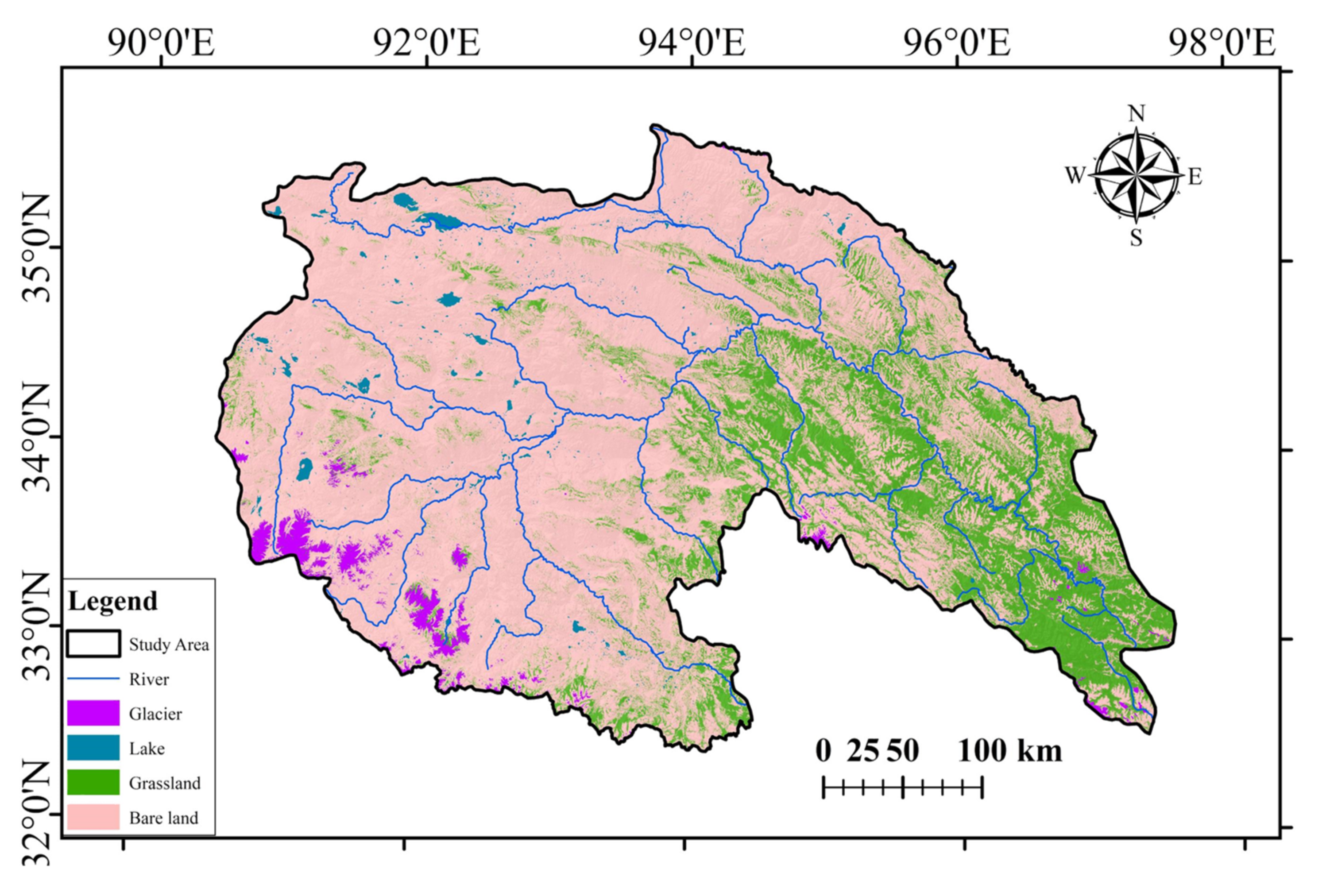
2.1. Study Aera and Data Source

2.1.1. Study Aera

The headwaters of the Yangtze River are located in the hinterland of the Qinghai-Tibet Plateau. Figure 1a,b show the location of the study area on the Qinghai-Tibet Plateau and in the Yangtze River Basin. The geographical coordinates of the study area are longitude 32°30′~35°35′E, latitude 90°43′~96°45′N, and the basin covers an area of approximately 138.2 × 10³ km2 [43]. As the geomorphological and drainage map of the headwaters of the Yangtze River shows (Figure 1c), there are various landforms in the basin, which include mountains, valleys, basins, lakes, and marshes. The Qinghai-Tibet Plateau climate system is a typical continental plateau climate, which is characterized by alternating wet-hot and dry-cold seasons, and the precipitation varies greatly with the altitude [44]. Glaciers are concentrated in the headwaters of the Yangtze River, which are mainly distributed in the Keladandong, Gaqiadirugang, and Gangqin snow mountain group. The largest areas covered by glaciers are found in the Dangqu Basin, followed by the Tuotuo River Basin; the smallest is located in the Chumar River Basin [45,46]. Furthermore, an interchange of materials and energy is constantly occurring between the glaciers, lakes, grasslands, and bare land [47].

2.1.2. Data Source

In this paper, the experimental dataset was produced from “Sentinel-2” high-resolution multispectral images, which were mainly used for monitoring the land environment, terrestrial vegetation, land cover, and watershed environment. This images were especially advantageous in the target segmentation in long-time series. The “Sentinel-2” images in this article were downloaded from the Copernicus Open Access Hub [48]. In order to comprehensively study the dynamic effects and the ecological stress of the eco-environment, the “Sentinel-2” images selected were mainly taken in July when the glacier line was the lowest. When the images were poor quality, such as at times of high cloud cover, they would be replaced by images taken in June and August [49,50].

2.2. Model

2.2.1. DeepLab V3+ Network

The semantic segmentation of remote sensing images is a full-pixel classification task, which includes categorical information and location information [51]. The traditional object-oriented segmentation algorithm uses low-level semantic information, such as the color, texture, and shape of the image being segmented [52], which is lacking intermediate semantics, such as pixel contrast and orientation. DeepLab V3+ introduced an encoder–decoder, which is commonly used to integrate multiscale information [53,54]. The decoder combines the up-sampling results of the depth map with shallow features [55]. Ultimately, the layer features are used to optimize location information that cannot be retrospectively sampled (Figure 2); the decoder up-samples the depth features and combines them with the shallow features [56,57]. The DeepLab V3+ network uses up-sampling to reconstruct the feature image, the results of which can include the classification and location information of glaciers, lakes, grasslands, and bare land [58,59].

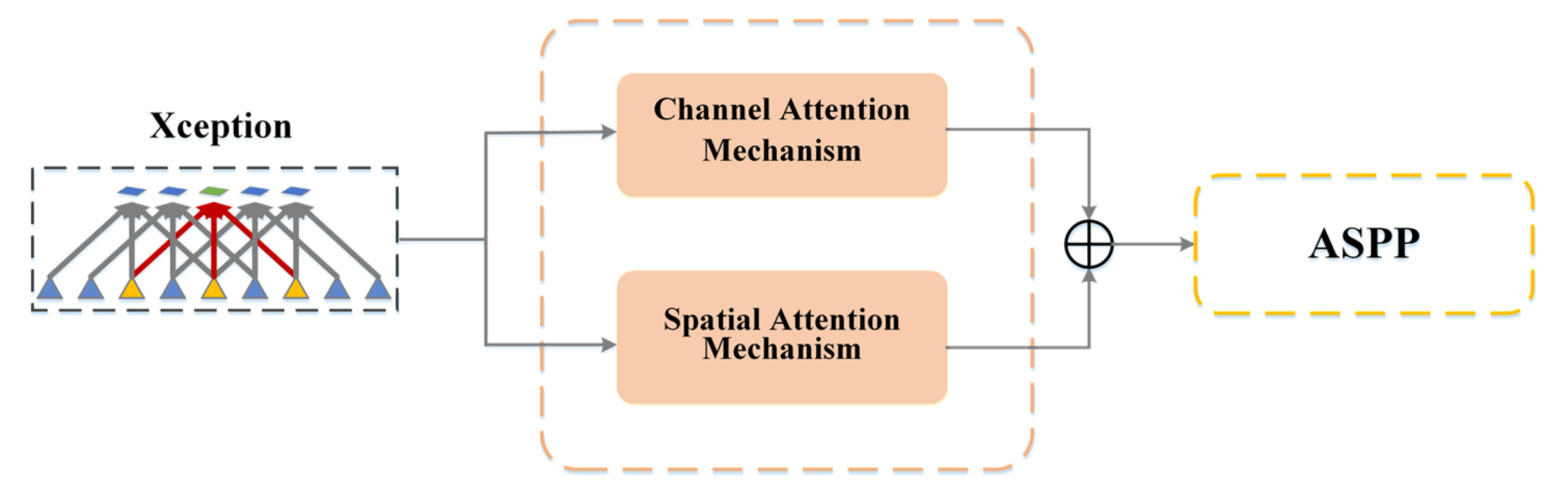
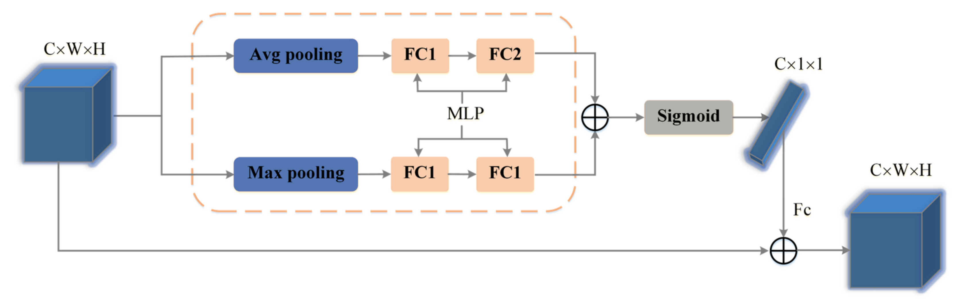
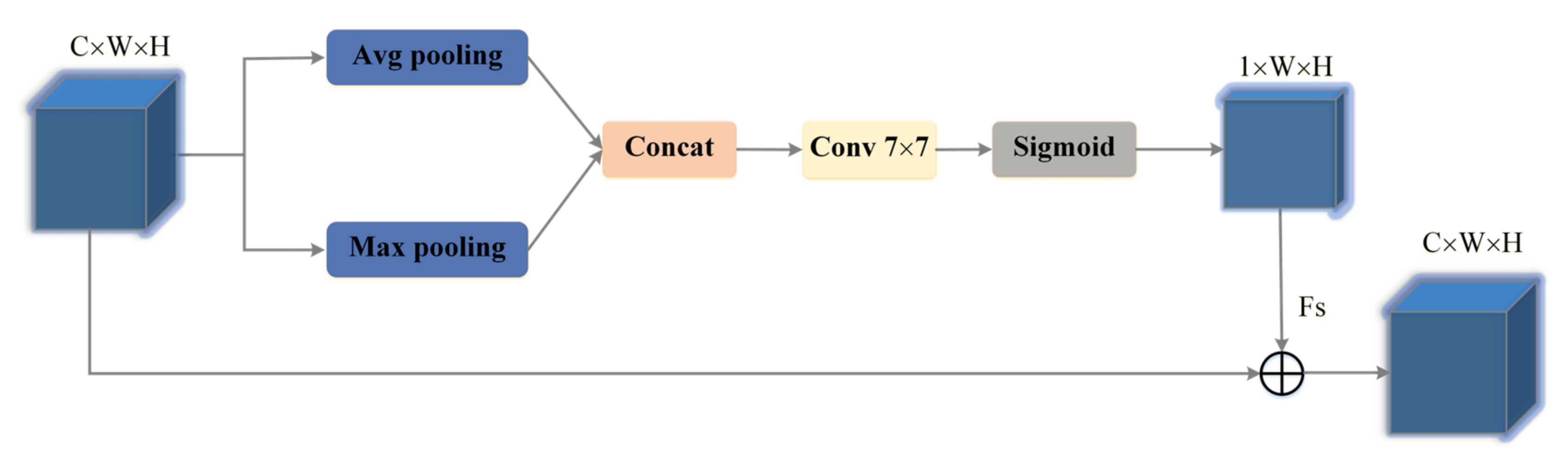
2.2.2. Improved DeepLab V3+ Model

DeepLab networks usually integrate shallow features with deep features, thus obtaining the high-level semantics between pixels and entity categories [60]. The encoder mainly extracts the depth feature information of the image, which is the key to achieving high-precision semantic segmentation. The encoder is mainly composed of DCNN and Atrous Spatial Pyramid Pooling (ASPP). We added the Double Attention Mechanism (DAM) to the ASPP module, so as to reduce accuracy loss (Figure 3). The specific operation is as follows: First, the global dependency relationship between features is captured in the spatial dimension and the channel dimension of features, respectively, to capture the context feature information and enhance the expression ability of features [61]; Then, the output of the two attention modules is added to further improve feature representation; Finally, a more accurate segmentation result is obtained.
The Channel Attention Mechanism (CAM) module selectively emphasizes the interconnected channel map by integrating the relevant characteristics in all channel maps. Therefore, this paper explicitly models the interdependence between channels by adding the CAM module. As Figure 4 shows, the original input feature map is multiplied by elements to obtain the channel attention weighted map.
The Spatial Attention Mechanism (SAM) module selectively aggregates the features of each location through the weighted sum of features of all locations. Regardless of distance, similar features are interrelated (Figure 5). As a consequence, in order to establish a richer context between local features, the SAM module is introduced.

2.2.3. Accuracy Assessment

Pixel accuracy is an evaluation index with which to calculate the proportion of the true value matched by the predicted value [62]. The mean Pixel Accuracy (mPA) represents the proportion of the number of classification pixels for each class to the average [63]. The mean Intersection over Union (mIoU) uses the mean value to represent the ratio of the intersection and union of the predicted set to the true set of the correct classification for each class [64]. The Kappa coefficient represents the coincidence degree between the classified image and the reference image, and it is an objective evaluation standard to test their consistency [65]. Both the mPA and mIoU are between 0 and 1, and the Kappa also usually falls between 0 and 1. Therefore, the closer the value is to 1, the better the semantic segmentation performance will be. The above three indicators are widely used in the evaluation of image semantic segmentation accuracy because of their simplicity and representation. All calculation formulae are shown below:
mPA   = 1 N i = 1 N n ii i = 1 N j = 1 N n ij
mIoU   = 1 N i = 1 N n ii j = 1 N n ij + j = 1 N n ji   n ii
Kappa = p o   p e 1     p e
where, N represents the total number of semantic segmentation classes, and nij is the pixel of class i divided into class j. The po is the number of the correctly classified samples divided by the total number of samples, and pe is the number of the misclassified samples divided by the total number of samples.

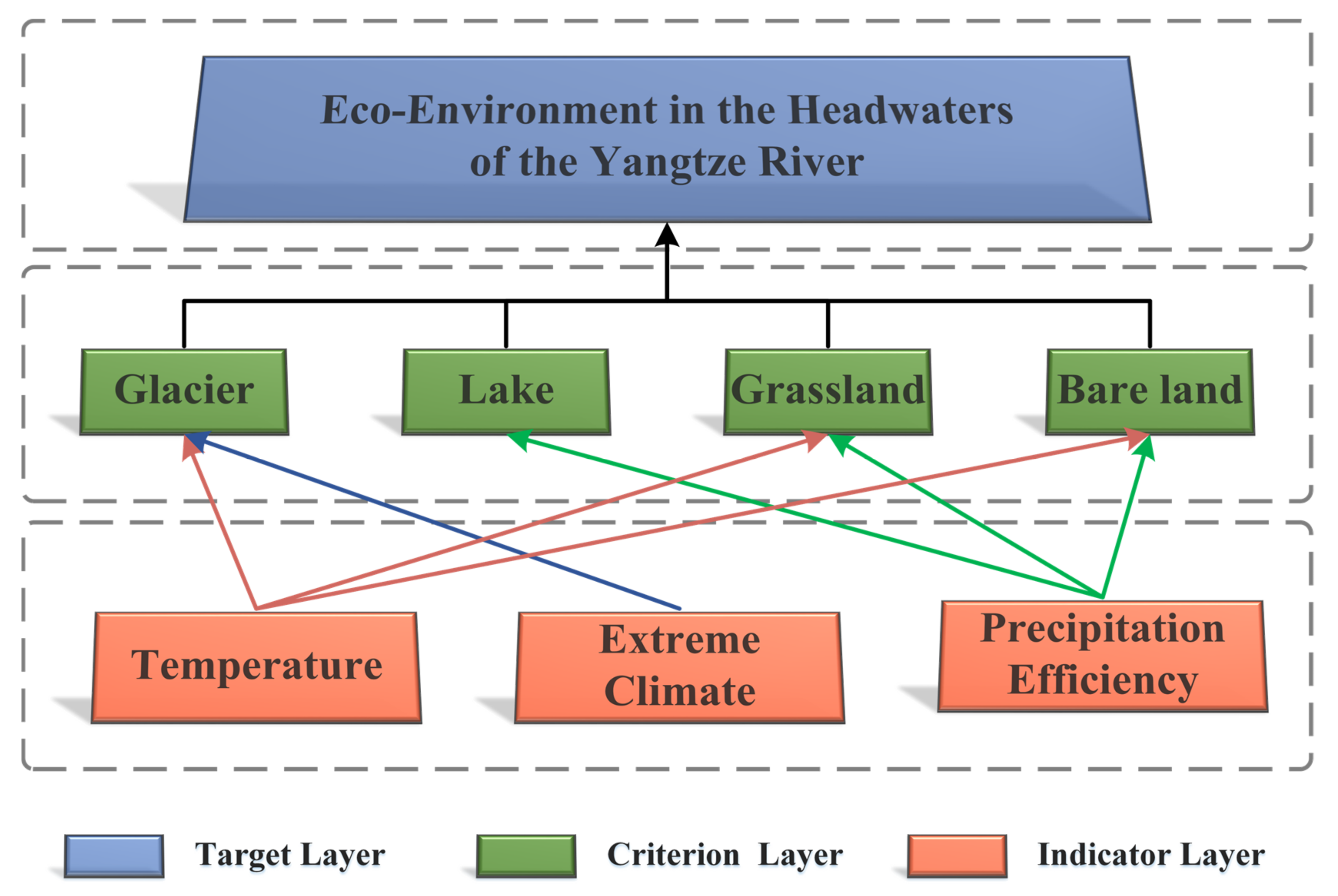
2.2.4. Elements Spatial Analysis

On the basis of the accurate extraction of eco-environment elements, a quantitative analysis of the spatial distribution characteristics and spatial relations can be conducted. Landscape connectivity is mainly controlled by the spatial distribution characteristics and spatial relationships of eco-environment elements, which provided the foundation from which to study the dynamic effects and ecological stress in the study area. Among them, Landscape Fragmentation (LF) and Shannon’s Diversity Index (SHDI) were used for the quantitative description [66]. The calculations of SHDI and LF were performed according to Formulas (4) and (5). LF refers to the process through which the landscape, from a single, homogeneous, and continuous whole, tends to become a complex, heterogeneous, and discontinuous patched mosaic [67]. LF reflects the complexity of the landscape spatial structure and the degree of interference caused by natural or human factors. SHDI is a measurement index based on information theory, the serious fragmentation of the landscape, and the lower mobility of the patches. This provides the conditions for the transformation and development of eco-environment analyses, from qualitative to quantitative, from static to dynamic, and from process to model. We propose the EF and the EIC based on the LF and SHDI to calculate eco-environment element connectivity [68,69,70]; the calculations were performed using Formulas (6) and (7).
LF   = N i A i
where, N i is the number of patches of landscape i, and A i is the total area of landscape i.
SHDI   = i = 1 S p i ln p i
where, S is the classes of landscape, and p i is the proportion of i landscape to the total landscape.
EF = 1 nm i = 1 n j = 1 m N ij A ij
where, n is the number of eco-environment elements, m is the number of classification scales, and N ij and A ij are the numbers and the areas of elements belonging to the m scale in class i, respectively.
EIC = i = 1 n j = 1 m ( q ij ln ( q ij ) ) i = 1 n ( q i ln ( q i ) )
where, n is the number of eco-environment elements, m is the number of classification scales, q ij is the proportion of the j scale to the total number of class i, and q i is the proportion of i element to the total elements.

3. Results

3.1. Experiment Data and Parameter

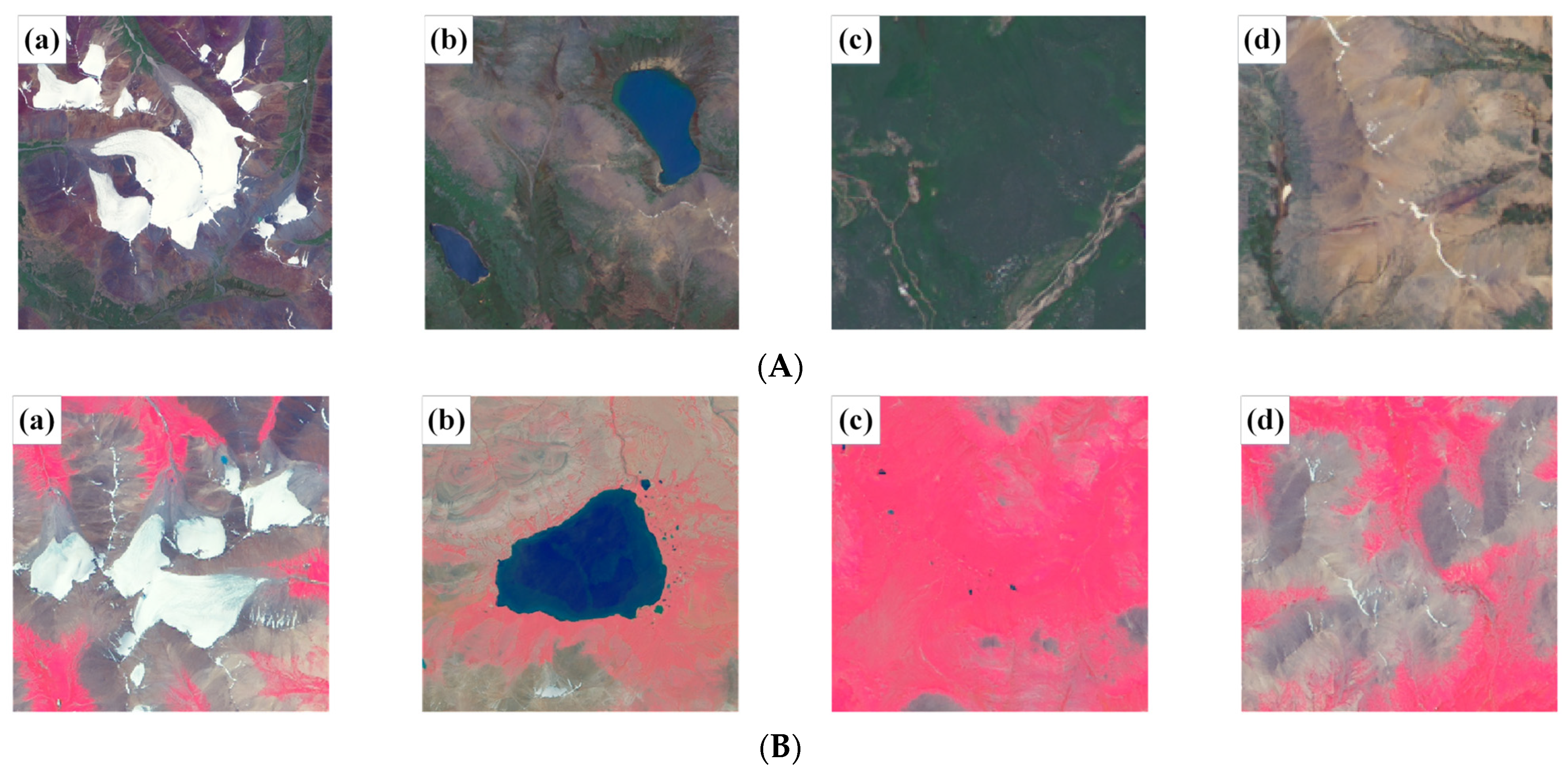
3.1.1. Identification Index

After radiation calibration and atmospheric correction processing, the radiation errors caused by atmospheric scattering and absorption in the “Sentinel-2” raw images were eliminated [71]. The samples obtained based on “Sentinel-2” images were selected to be exported into TIF datasets. We converted all samples from TIF format to IMG format, which was used as the input for the training [72]. According to the distribution, the identification indexes of eco-environment elements were established according to the surface reflection and spatial texture characteristics, which were used to establish a label system that the network was able to recognize [73]. The interpretation marks established in the eco-environment elements were verified in related articles. This laid the foundation for building sample sets (Figure 6). The interpretation signs are summarized as follows:
(1)
Glaciers have a relatively simple textural structure, with a bright tone in both true-color and false-color images. Glaciers have a high contrast with the surrounding environment. In regards to morphological structure, glaciers often appear with an arc-shaped boundary;
(2)
Water has a certain boundary in the remote sensing image. According to the mineral content, the depth of the water, and the imaging time, water is predominantly cyan or bluish green both in true-color and false-color images;
(3)
Grassland and bare land, as the largest portion of the study area, are relatively similar in terms of spatial distribution. In true-color images, grassland mainly has a green color and bare land mainly a tan and flesh pink color. In false-color images, grassland mainly has a red color, and bare land mainly has a tan and flesh pink color similar to in true-color images.

3.1.2. Sample Sets

There was a total of 5717 pictures annotated with eco-environment elements. All pictures with resolution of 10 m were collected from the Source of Three Rivers (Table 1, in which the number and size are non-dimensional). Sample sets were divided into mutual exclusion training sets and test sets, and the validation sets were included in the training sets. We trained the model on the training sets, and verified the accuracy of the extractive effect using the validation sets. We implemented model selection using the validation sets. Once the best parameters were identified, final training could be performed on the test sets. Finally, the model was used to train the remote sensing images in the study area, and the classification of eco-environment elements was obtained. The eco-environment elements in the training sets and test sets demonstrated spatial differences and feature similarity, so the generalization performance of the model was well reflected. The ratio of training sets to test sets was 7:3. The dataset ratio R of training sets to validation sets is discussed in Section 4.3. Eco-environmental element monitoring research was conducted in the study area.

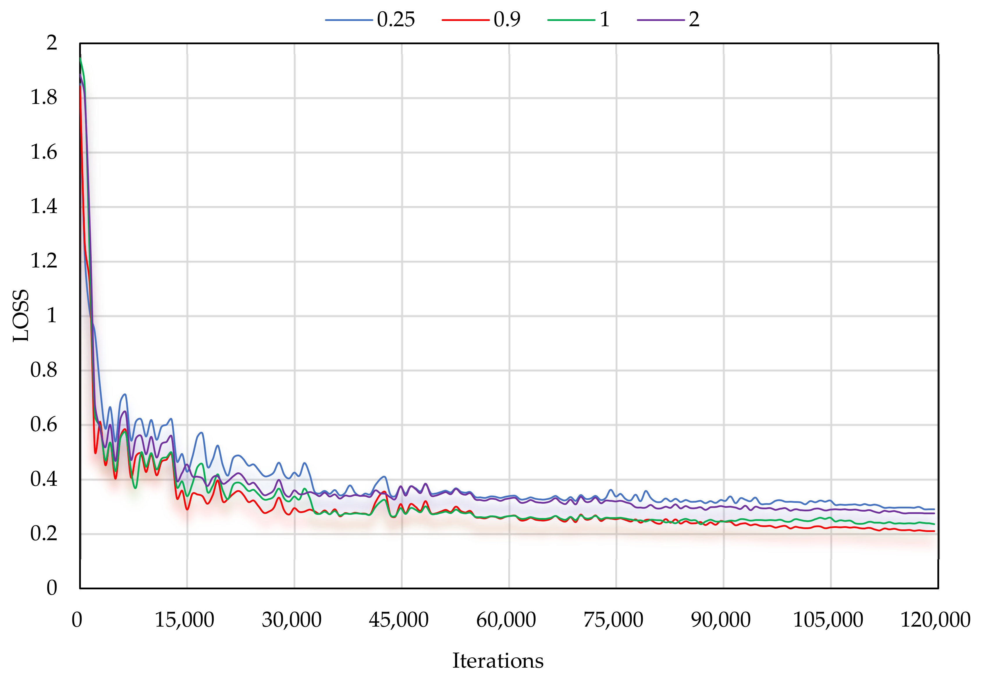
3.2. Parameters Setting

3.2.1. Parameters Index

In the process of pixel segmentation of the eco-environment elements, the parameter selection of the dataset ratio R of the training sets to validation sets, the learning rate Y t , and batch_size had the most impact on performance [74]. In this paper, the control variable method was used to comprehensively select the three parameters. We selected the momentum optimizer, which uses the objective function to optimize training parameters. The appropriate learning rate causes the optimizer to optimize the model parameters more effectively, and the poly learning rate was selected for optimization [75]. The training objective function includes the log-likelihood function and L2 regularization term [76,77,78]. The results calculated by Softmax represent the difference between the true label and the predicted label, and the regularization term can prevent overfitting to a certain extent [79]. The formulae are as follows:
Y t = X ( 1   t T ) p
Loss   = 1 K n = 1 N i = 1 K y true ni log y pred ni
where, Y t is the current learning rate, X is the initial learning rate, t is the current training times, and T is the total number of trainings. K is the total number of pixels with labels, N is the number of classes, y true ni is the probability of pixel i corresponding to class N, and y pred ni is the probability of pixel i being output by the network corresponding to class N.

3.2.2. Parameters Selection

As a result of the influence of computer GUP memory, the batch_size was fixed at 10 during the experiment. When Y t = 0.9 and the proportion of samples in the training sets and validation sets was 6:4, the training accuracy and validation accuracy were the highest (Table 2), so the parameter R was taken as 6:4. Using the same method, we set batch_size = 10, R = 6:4, and Y t as 0.25, 0.9, 0.1, and 2, respectively, for training. In the initial stage of training, the Loss values of all curves were large. With the increase in iterations, the Loss value continued to oscillate and decline slowly. When the model was iterated 60,000 times, the Loss values of all curves were basically stable and remained so until the end of the iteration. When Y t = 0.9 , the Loss value finally stabilized at 0.21, so the parameter Y t was taken as 0.9 (Figure 7). In order to avoid the introduction of a large amount of noise into the parameters, the remaining parameters that had little influence on the model were used in the training with their initial values. The final parameter values are shown in Table 3.

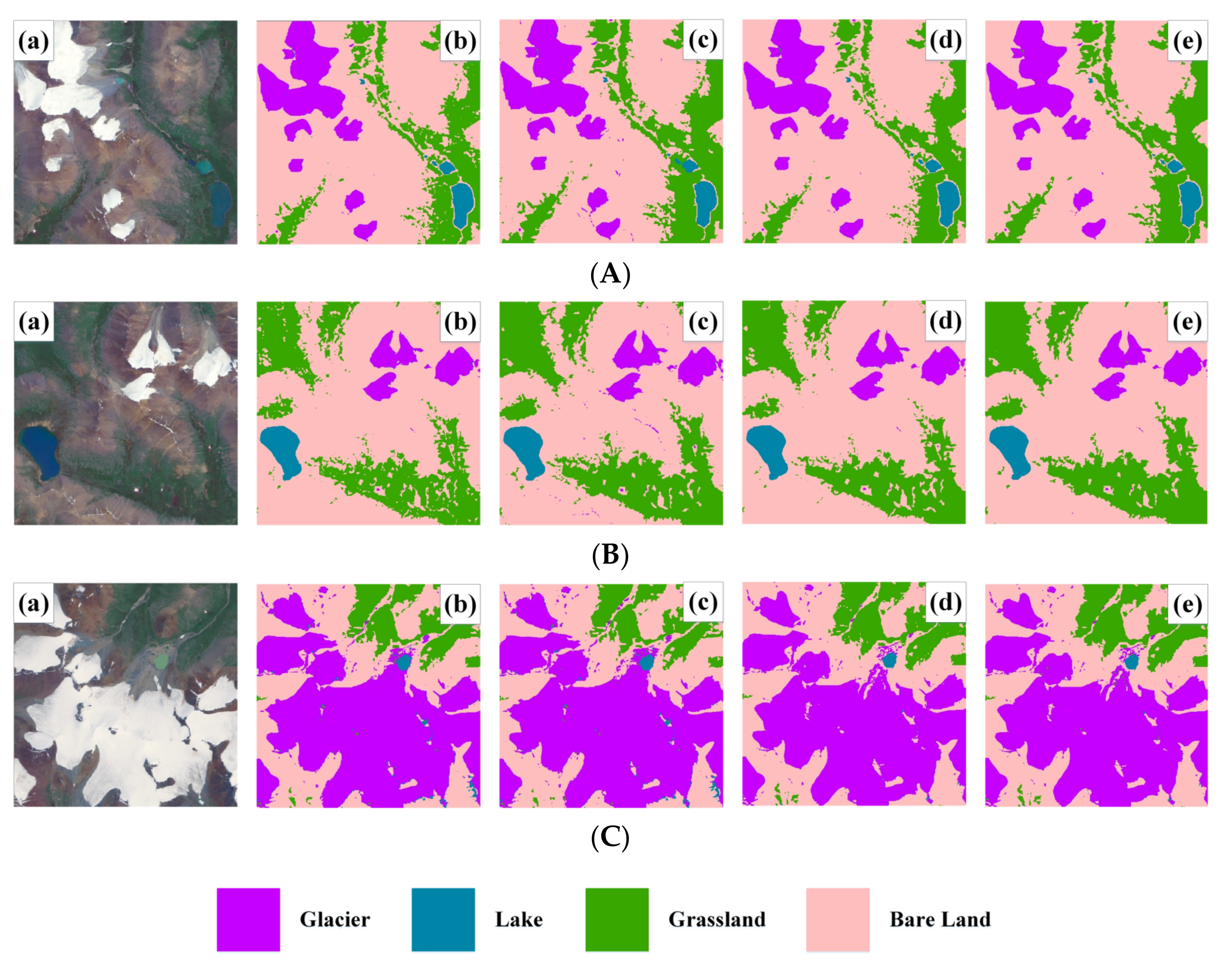
3.3. Results Analysis

In order to verify the performance of the DeepLab V3+ network and demonstrate its application value, we validated DeepLab V3+ and Support Vector Machine (SVM), UNet, and DeepLab V3 on the sample sets. The automatic identification results of different models are shown in Figure 8. Generally speaking, the classification based on the SVM and UNet methods demonstrated better extraction integrity. The eco-environmental elements were prone to misclassification. As compared with the other four methods, the extraction results of the eco-environment elements based on the DeepLab V3+ network exhibited better performance in terms of comprehensive positioning accuracy and extraction boundary integrity. The comparison results are summarized in the following:
(1)
SVM extracted the pixels that conformed to the glaciers, lakes, grasslands, and bare land to a certain degree. However, there was obvious misclassification in the extraction results of different classes. For this method, the mPA and Kappa of the SVM segmentation results were the worst, with values of 0.463 and 0.641, respectively. The segmentation results of SVM are greatly affected by other surface reflectivity features;
(2)
The extraction results of UNet were greatly affected by background interference and spectral features, and some frozen lakes were mistakenly classified as glaciers. As a result of the high altitude, some lakes were still frozen during this period, but they had various different shape characteristics as compared to glaciers. As the Table 4 shows, the lowest index of mIoU was recorded for UNet, indicating that this method could not semantically segment the eco-environment elements well. As a result, the extraction of grassland was more fragmented and the accuracy was lower;
(3)
DeepLab V3 had a good ability to identify the eco-environment elements. However, it needed to train many times to achieve better results for complex eco-environment elements. DeepLab V3 was able to accurately classify the eco-environment elements in the spatial position through high-cost training;
(4)
The performance of each index for DeepLab V3+ was superior to those of DeepLab V3, with the mAP, mIoU, and Kappa of the former being 0.639, 0.778, and 0.825, respectively. The extraction results based on DeepLab V3+ had a complete structure and obvious edge features, and it did not produce missing or wrong divisions for small areas of grassland. The DeepLab V3+ method demonstrated a good ability to distinguish the eco-environment elements in the headwaters of the Yangtze River.

4. Discussion

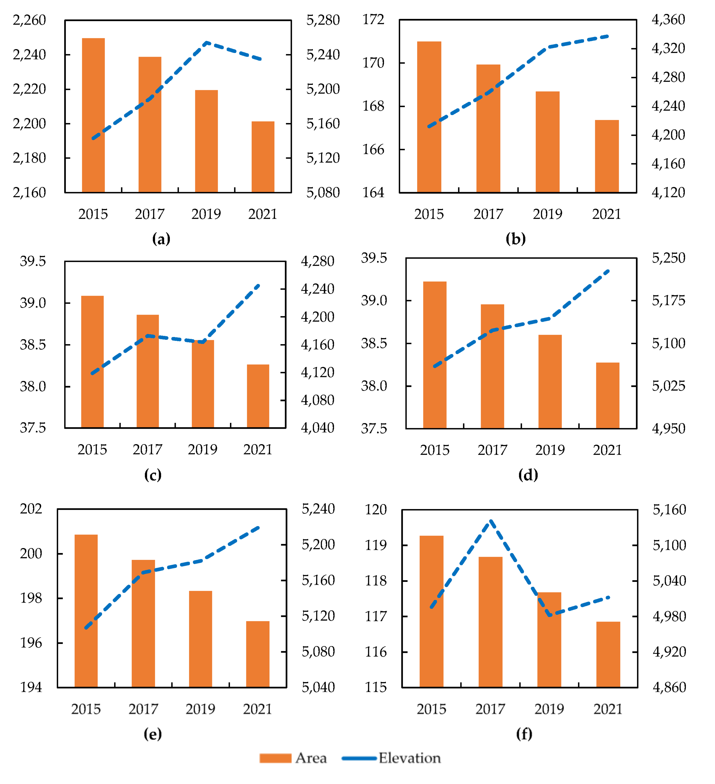
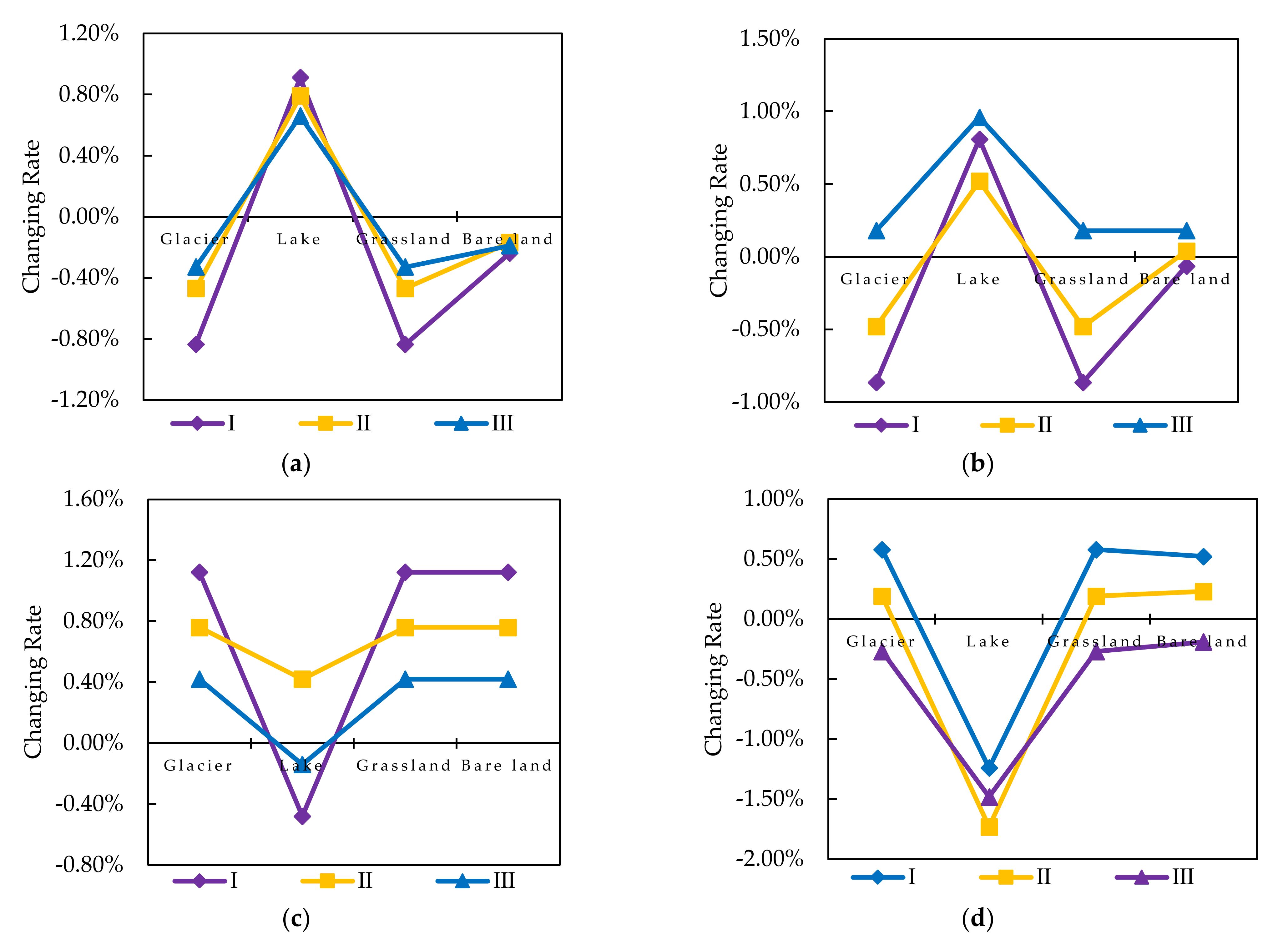
4.1. Elements Changes

Using the DeepLab V3+ network, each pixel was accurately extracted. The eco-environment elements extraction experimental results were pieced together from the original geographic information, and each pixel had its own function because of the spatial relationship. The changes in these elements in the study area under the different space-time states and scales of coverage were used to produce comparative statistics, as illustrated in Table 5. In this paper, every two years was set as an interval (Table 6). Taking Yushu City as an example, we found that the glaciers, lakes, grasslands, and bare land underwent constant development and changes. In the headwaters of the Yangtze River, the glaciers, lakes, grasslands, and bare land are interdependent and interlaced.

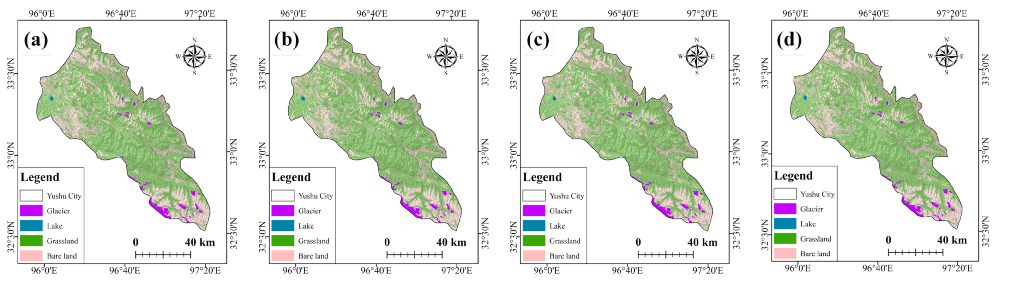
4.1.1. Glaciers Changes

As shown in Figure 9, the glaciers are mainly distributed to the southwest of Golmud City. There are other glaciers scattered in Southern Zaduo County, Southern Zhiduo County, Sortheastern Yushu City, Northern Qumalai County, and Western Chengduo County (Figure 10). By studying the distribution of glaciers, the overall trend of glacier change could be obtained. In general, the glaciers in the study area were decreasing and breaking up during the study period.
(1) The total area of glaciers in each region is shrinking. The total area of glaciers in the initial stage (2015) was 2818.98 km2, and the areas of glaciers in Golmud City, Yushu City, Chengduo County, Qumalai County, Zaduo County, and Zhiduo County were 2249.58, 170.99, 39.08, 39.22, 200.84, and 119.27, respectively. However, in 2021, the areas were 2201.33, 167.36, 38.26, 38.37, 196.97, and 116.85, respectively.
(2) The decrease in the glacier area was accompanied by an increase in the snowline altitude. As shown in Figure 11, the elevation distribution and change rate of the snowline altitude in each region was not the same (the changing rate was non-dimensional), with the snowline altitude equaling 5234, 4322, 4164, 5144, 5218, and 4982 m in 2021.
(3) The glacier changes at different scales in the headwaters of the Yangtze River generally exhibited different change rates, as shown in Figure 12. The number of large-scale glaciers in the study area remained unchanged, and the downward trend for medium-scale glaciers was slight as compared with the dramatic change seen in smaller-scale glaciers, as shown in Figure 13 (the unit of area is square kilometers (km2), while the unit of elevation is meters (m)).

4.1.2. Lakes Variation

Lakes are mainly located in the central or western regions of the study area, and there are relatively few lakes in Eastern Zhiduo County, Eastern Qumalai County, and most parts of Yushu City. Geographically, most lakes in the headwaters of the Yangtze River are located in uninhabited areas with high altitudes and are less affected by human activities. In the three periods, the changing trend for scales was different from that of area. Generally, increasing temperature and precipitation were conducive to the expansion of the area of glacier-replenished lakes.
As shown in Figure 14 and Figure 15, there were 4072 smaller-scale lakes, 89 small lakes, 15 medium lakes, and 2 large lakes in 2015. In the initial stage, the total number of large lakes was two, representing 21.28% of all lakes, and the proportions of medium-scale, small-scale, and smaller-scale lakes were 34.98%, 20.87%, and 22.87%, respectively. By 2021, the number of large-scale, medium-scale, small-scale, and smaller-scale lakes was 2, 17, 93, and 3927, accounting for 23.64%, 37.27%, 20.67%, and 18.42% of the total area. As a result of the influence of various factors, the total number of lakes continued to increase, but the quantity of large-scale lakes remained unchanged, and the quantity and area of small lakes was reduced to different degrees.

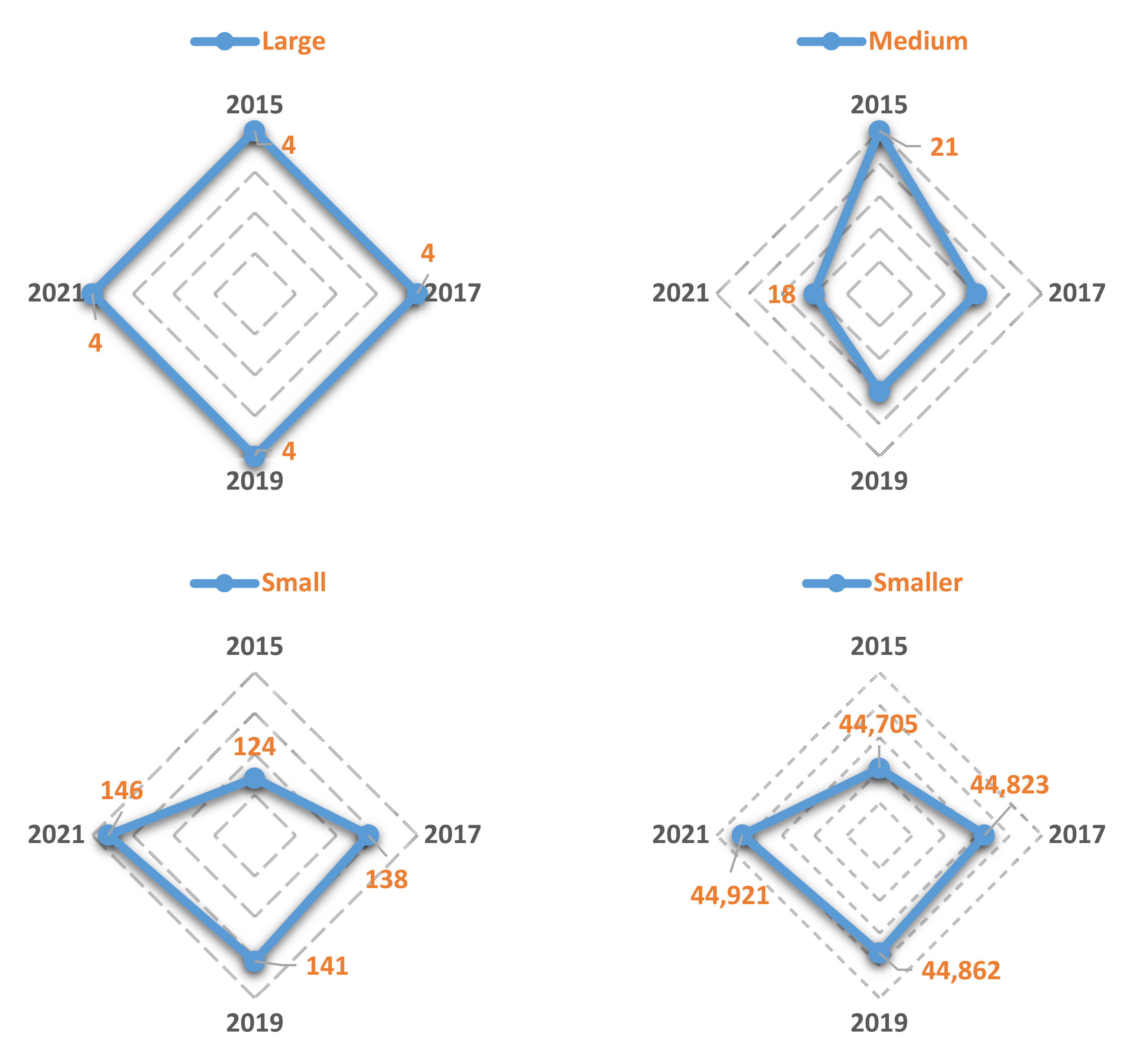
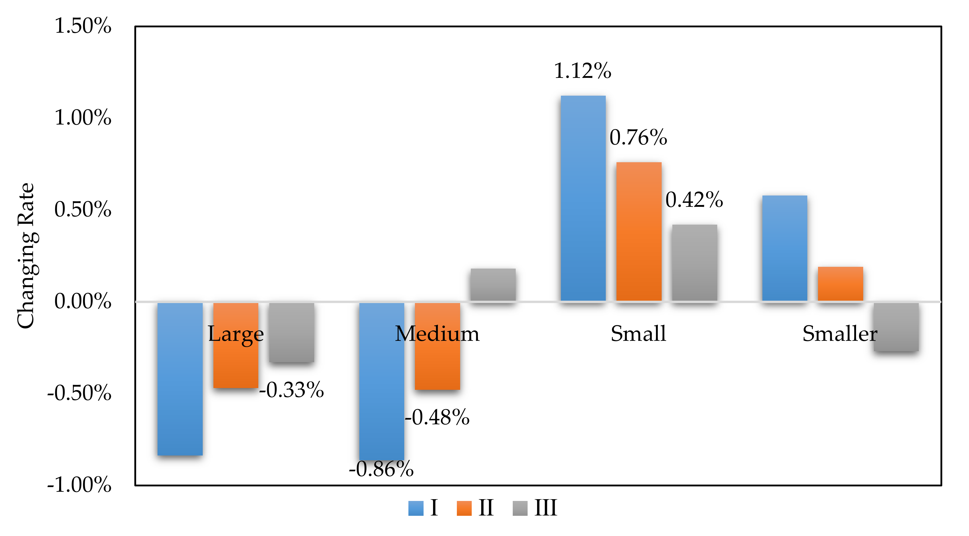
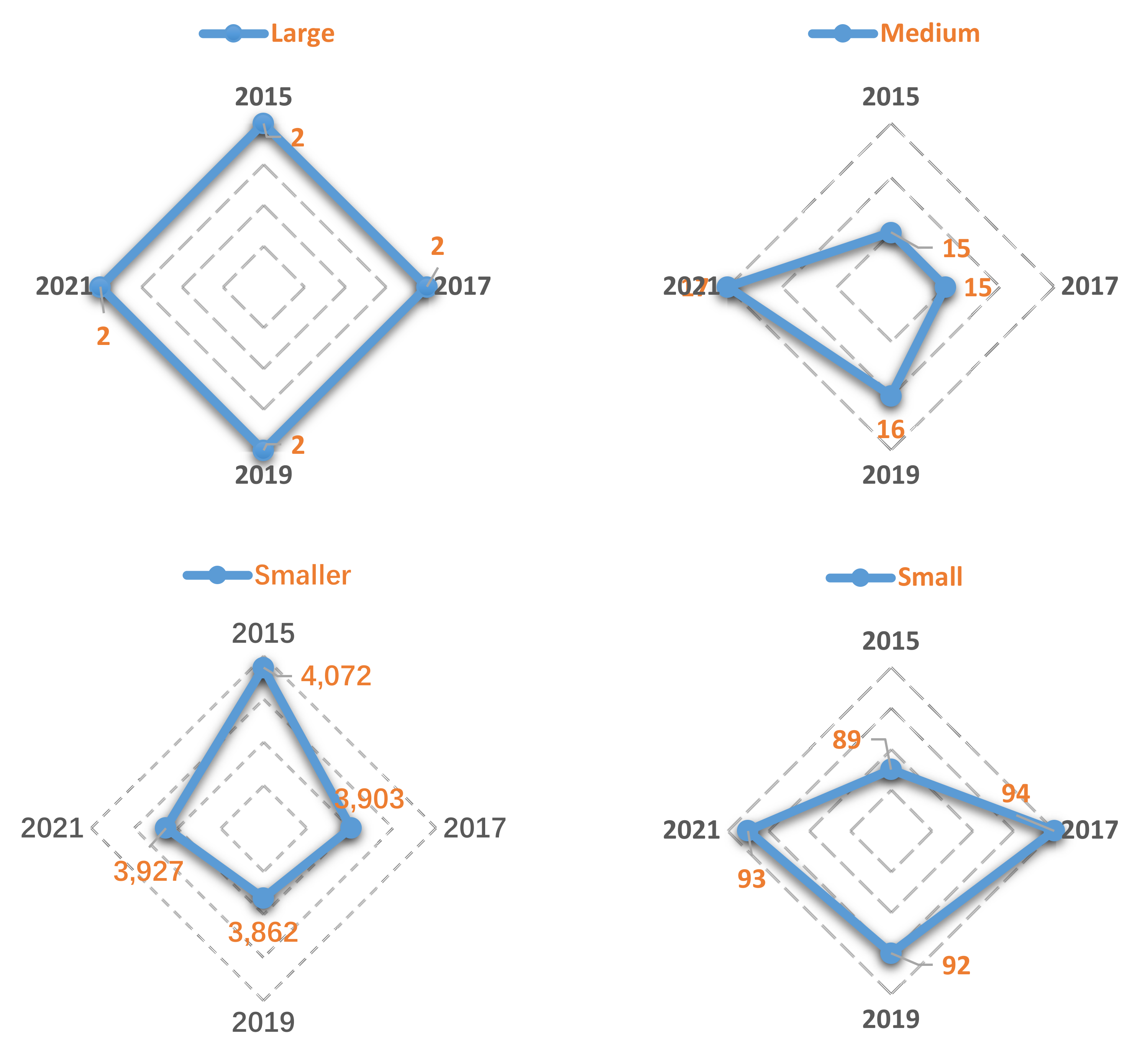
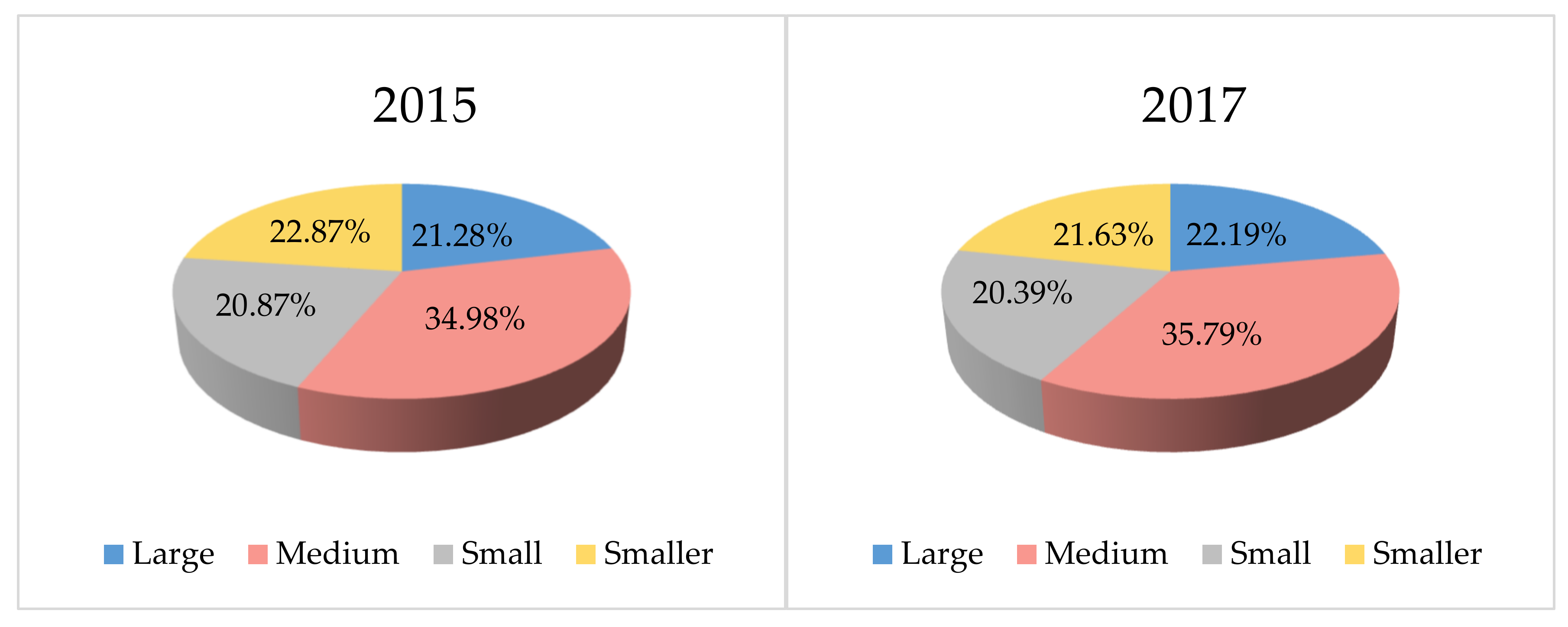
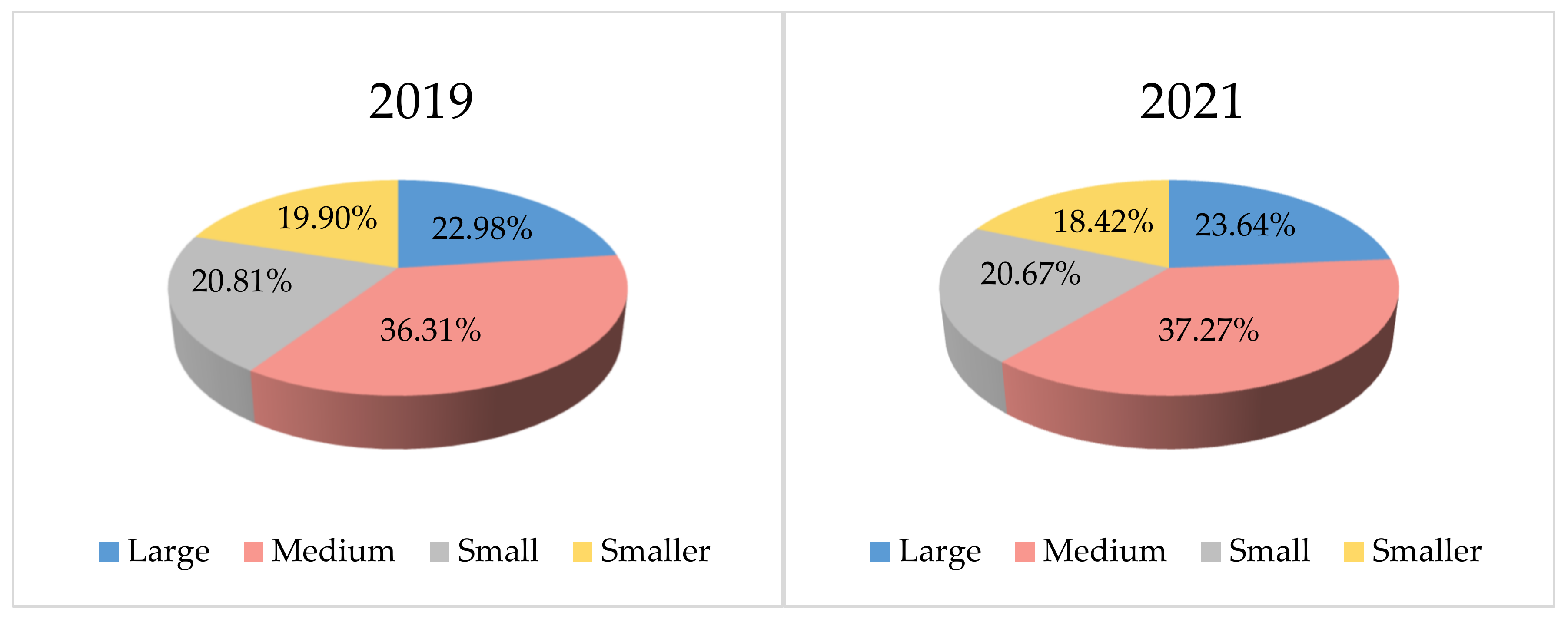
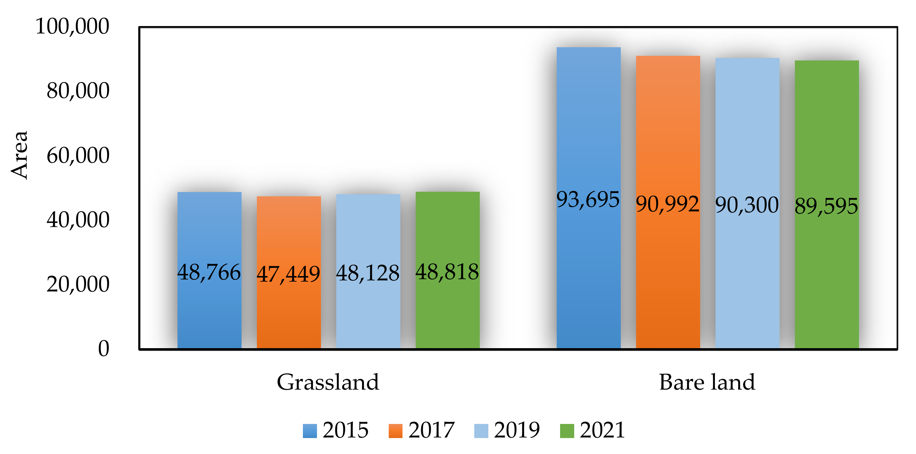
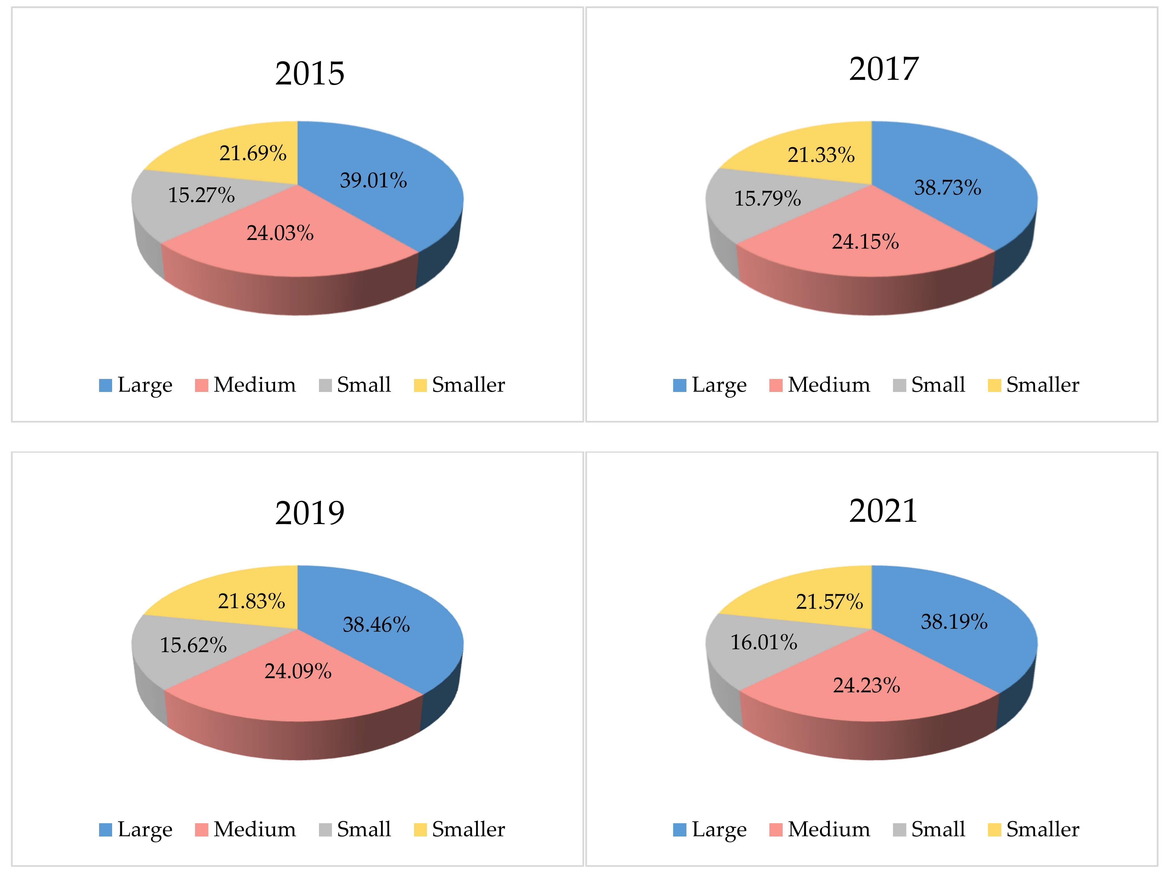
4.1.3. Grasslands and Bare Land
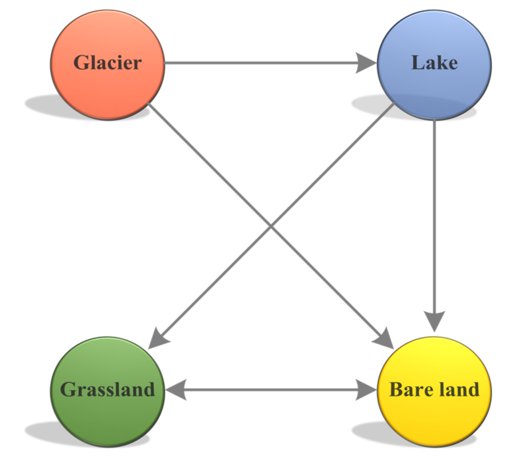
The grasslands represent the main area covered with vegetation in the headwaters of the Yangtze River and the coverage is an important index to measure the surface vegetation coverage in the study area. As a result of the typical continental plateau climate, the sparsely covered and uncovered vegetation areas, which we called bare land, were extremely fragile and sensitive, with complicated changes in vegetation cover.
(1) Grasslands are widely distributed in the Eastern Zhiduo County, Eastern Qumalai County, Western Chengduo County, Southeastern Zaduo County, and most parts of Yushu City. In this region, bare land mainly exists in the alpine desert areas, such as most parts of Golmud City, Northern Qumalai County, and Northern Zaduo County. According to the statistics in Figure 16 (the unit of area is square kilometers), the area of grassland in the study area was 48,796 km2 in 2015, and 47,448, 48,127, and 48,817 km2 in 2017, 2019, and 2021, respectively, exhibiting a slight increase overall.
(2) According to the statistics in Table 7 and Figure 17, small-scale and smaller-scale grassland areas increased and the larger-scale areas decreased slightly. However, the bare land area did not continue to increase as originally envisaged. A comprehensive comparison showed that the grassland coverage in the study area was directly or indirectly affected by unique climate factors.

4.2. Dynamic Effect

Global climate change affects the moisture and energy exchange between atmosphere and earth systems and finally influences the distribution of eco-environment elements [80,81]. As an individual whole, the study area is frequently involved in complex material circulation and energy flow with the outside world. The headwaters of the Yangtze River are a community of life. The system scientifically guides mankind to explore the endogenous relationship between human beings and the natural environment in a highly condensed and vividly illustrative way. Therefore, this paper attempts to analyze the dynamic effects of this region from a systematic, holistic, and multiscale perspective.

4.2.1. Systematic

The community of life in the headwaters of the Yangtze River has a distinct gradation. The indicators of different dimensions can be divided into the indicator layer, the criterion layer, and the target layer from low to high, and there is a clear logical relationship between different levels, i.e., the dynamic systematic effects [82]. As shown in Figure 18, the individual eco-environment element is the criterion layer of the system, and it reflects a certain aspect of the development of the community of life in the headwaters of the Yangtze River, which is represented by the target layer [83]. Ultimately, the comprehensive eco-environment elements reflect the overall situation of the region. The indicator layer mainly includes temperature, extreme climate, and precipitation efficiency. There are differences in the location, function, and other attributes of different elements in the eco-environment, and there are also differences in the basic characteristics, such as the structure and function of different types of eco-environment.

4.2.2. Holistic

There are relationships, interplay, and restrictions in eco-environment elements. Once the eco-environment is damaged to a certain extent, it will affect the normal operation of the whole eco-environment. From 2015 to 2021, as Table 8 shows (the unit of area is km2), the areas of glacier and bare land reduced from 2818.99 to 2759.04 and from 93,695.39 to 89,595.21, respectively. Moreover, the areas of lake and grassland increased from 1424.37 to 1532.69 and from 46,766.02 to 48,817.83, respectively. The overall eco-environment elements are constantly transforming. Taking the glaciers as an example, changes in these areas can cause variation in the energy exchange between the atmosphere and earth systems and the snowmelt runoff. The continuous melting of glaciers leads to an increase in runoff, which is conducive to the expansion of glacial-replenished lakes and grasslands. The increase in lakes has the most direct effect on the development of the surrounding grassland ecosystem. Furthermore, the changes in grasslands and bare land can affect water retention and groundwater storage in soil. As shown in Figure 19, the holistic of dynamic effects in the headwaters of the Yangtze River are ultimately reflected in the interaction and mutual development of the overall eco-environment elements.

4.2.3. Multiscale

There are large differences in the structural complexity and functional diversity of ecosystems at different scales. The change rates of various eco-environment elements in the headwaters of the Yangtze River at different scales in the three time periods are shown in Figure 20. The area change rate of each scale element in the three periods exhibits a similar trend. With the increase in the change rate of the smaller-scale glaciers, the smaller-scale lakes, the grasslands, and bare land generally increased. Thus, it can be concluded that the changes in areas of glaciers, lakes, and grasslands were consistent in the smaller-scale. This also appears in small-scale, medium-scale, and large-scale eco-environment element changes. There are differences in the position, function, and other attributes of the eco-environment elements on different scales in the ecosystem, and the results of their interaction also differ.

4.3. Ecological Stress

The ecological stress in the headwaters of the Yangtze River represents a natural disturbance to the structure and function of the ecosystem caused by human action, and this direct or indirect interference often exceeds the scope of ecological rehabilitation [84]. In this paper, the ecological landscape was introduced in order to scientifically define ecological stress [85,86]. Ecologically, the landscape is a spatially heterogeneous region that repeatedly appears in a similar form, and it is a natural complex with classification significance [87]. Therefore, the different eco-environment elements are also the different landscapes that have different continuities in terms of spatial structural features.
With the intensification of global warming and the increasing intensity of the Indian summer monsoon, the climate in the headwaters of the Yangtze River exhibits a warm and humid trend. Therefore, the eco-environment in this area has experienced drastic changes. Specifically, rising temperatures lead to accelerating glacial melting, a reduction in permafrost, fluctuations in the number and areas of small lakes, and serious desertification of the land. As Figure 21 shows, as time goes on, although the trends of the two differ, the EF and EIC keep increasing, which indicates that, during to the combined effect of nature and humans, the eco-environment elements are oriented towards complex, heterogeneous, and discontinuous processes (EF and EIC are non-dimensional). Eco-environment element fragmentation is serious, and the community of life has a relatively low level of connectivity between the eco-environment elements.

5. Conclusions

The headwaters of the Yangtze River are a complicated system composed of different eco-environment elements, and there is constant multilevel and multiscale material circulation and energy exchange in such elements. On the basis of a series of studies on the dynamic effects of ecological stress on eco-environment elements, we came to the following main conclusions:
(1)
In the process of eco-environment element identification, the improved DeepLab V3+ network was used to efficiently identify glaciers, lakes, grasslands, and bare land elements on the dataset established by “Sentinel-2” remote sensing images in the headwaters of the Yangtze River. The mAP, mIoU, and Kappa of the improved DeepLab V3+ method were 0.639, 0.778, and 0.825, respectively, which demonstrate a good ability to distinguish eco-environment elements;
(2)
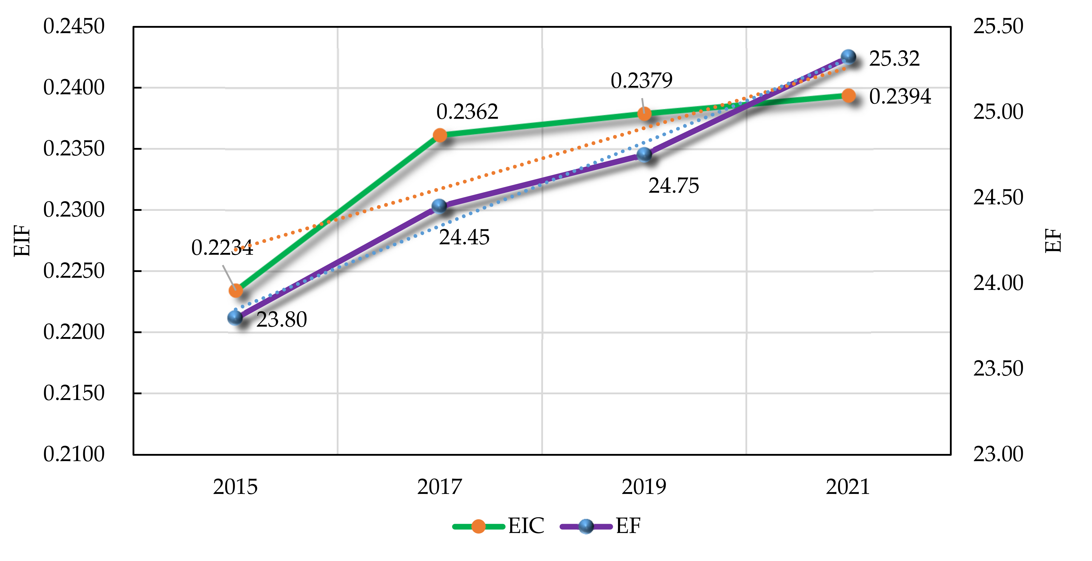
We propose using the EF and EIC to calculate the connectivity between eco-environment elements against the background of change and transformation. Between 2015 and 2021, EF gradually increased from 0.2234 to 0.2394, and EIC increased from 23.80 to 25.32, which indicates that the study area has a relatively low level of eco-environment elements connectivity. The eco-environment is oriented towards complex, heterogeneous, and discontinuous processes;
(3)
As a community of life, the study area is frequently involved in a complex material circulation and energy flow with the outside world. The eco-environment elements in the headwaters of the Yangtze River are a systematic, holistic, and multiscale whole within a constantly transforming system, and each of them is universally connected.

Author Contributions

Conceptualization, C.W.; Formal analysis, L.C.; Methodology, C.W.; Project administration, R.Z.; Software, L.C.; Supervision, R.Z.; Validation, C.W. and L.C.; Writing—original draft, C.W. All authors have read and agreed to the published version of the manuscript.

Funding

This research received no external funding.

Data Availability Statement

Due to the nature of this research, participants of this study did not agree for their data to be shared publicly, so supporting data is not available.

Conflicts of Interest

The authors declare no conflict of interest.

References

  1. Yue, W.Z.; Wang, T.Y. Rethinking on the Basic Issues of Territorial and Spatial Use Control in China. China Land Sci. 2019, 33, 8–15. [Google Scholar]
  2. Gao, H.; Feng, Z.; Zhang, T.; Wang, Y.; He, X.; Li, H.; Pan, X.; Ren, Z.; Chen, X.; Zhang, W.; et al. Assessing glacier retreat and its impact on water resources in a headwater of Yangtze River based on CMIP6 projections. Sci. Total Environ. 2021, 765, 142774. [Google Scholar] [CrossRef] [PubMed]
  3. Das, S.; Fime, A.A.; Siddique, N.; Hashem, M.M.A. Estimation of Road Boundary for Intelligent Vehicles Based on DeepLabV3+ Architecture. IEEE Access 2021, 9, 121060–121075. [Google Scholar] [CrossRef]
  4. Chen, B.; Zhang, X.; Tao, J.; Wu, J.; Wang, J.; Shi, P.; Zhang, Y.J.; Yu, C. The impact of climate change and anthropogenic activities on alpine grassland over the Qinghai-Tibet Plateau. Agric. For. Meteorol. 2014, 189–190, 11–18. [Google Scholar] [CrossRef]
  5. Cheng, G.D.; Wu, T.H. Responses of permafrost to climate change and their environmental significance, Qinghai-Tibet Plateau. J. Geophys. Res. Earth Surf. 2007, 112, F02S03. [Google Scholar] [CrossRef] [Green Version]
  6. Liu, J.; Chen, J.; Xu, J.; Lin, Y.; Yuan, Z.; Zhou, M. Attribution of runoff variation in the headwaters of the Yangtze River based on the Budyko hypothesis. Int. J. Environ. Res. Public Health 2019, 16, 2506. [Google Scholar] [CrossRef] [Green Version]
  7. Wang, J.; Schweizer, D.; Liu, Q. Three-dimensional landslide evolution model at the Yangtze River. Eng. Geol. 2021, 292, 106275. [Google Scholar] [CrossRef]
  8. Du, S.; Du, S.; Liu, B.; Zhang, X. Incorporating DeepLabv3+ and object-based image analysis for semantic segmentation of very high resolution remote sensing images. Int. J. Digit. Earth 2021, 14, 357–378. [Google Scholar] [CrossRef]
  9. Guo, B.; Luo, W.; Wang, D.L.; Jiang, L. Spatial and temporal change patterns of freeze-thaw erosion in the three-river source region under the stress of climate warming. J. Mt. Sci. 2017, 14, 1086–1099. [Google Scholar] [CrossRef]
  10. Makarevich, K.G. Hydrological aspects of the glacier regime in the north tien shan in the anomalously arid period of 1974–1978. Int. Assoc. Hydrol. Sci. Publ. 1982, 138, 43–50. [Google Scholar]
  11. Mellit, A.; Kalogirou, S. Artificial intelligence and internet of things to improve efficacy of diagnosis and remote sensing of solar photovoltaic systems: Challenges, recommendations and future directions. Renew. Sust. Energy Rev. 2021, 143, 110889. [Google Scholar] [CrossRef]
  12. Haefner, N.; Wincent, J.; Parida, V. Artificial intelligence and innovation management: A review, framework, and research agenda. Technol. Forecast Soc. 2021, 162, 120392. [Google Scholar] [CrossRef]
  13. Lary, D.J.; Alavi, A.H.; Gandomi, A.H. Machine learning in geosciences and remote sensing. Geosci. Front. 2016, 7, 3–10. [Google Scholar] [CrossRef] [Green Version]
  14. Bradley, B.A.; Mustard, J.F. Characterizing the landscape dynamics of an invasive plant and risk of invasion using remote sensing. Ecol. Appl. 2006, 16, 1132–1147. [Google Scholar] [CrossRef] [Green Version]
  15. Jiang, C.; Zhang, L.B. Climate Change and Its Impact on the Eco-Environment of the Three-Rivers Headwater Region on the Tibetan Plateau, China. Int. J. Environ. Res. Public Health 2015, 12, 12057–12081. [Google Scholar] [CrossRef] [Green Version]
  16. Menz, M.H.M.; Dixon, K.W.; Hobbs, R.J. Hurdles and opportunities for landscape-scale restoration. Science 2013, 339, 526–527. [Google Scholar] [CrossRef] [PubMed]
  17. O’Neill, R.V.; Hunsaker, C.T.; Jones, K.B.; Riitters, K.H.; Wickham, J.D.; Schwartz, P.M.; Goodman, I.A.; Jackson, B.L.; Baillargeon, W.S. Monitoring environmental quality at the landscape scale: Using landscape indicators to assess biotic diversity, watershed integrity, and landscape stability. BioScience 1997, 47, 513–519. [Google Scholar] [CrossRef] [Green Version]
  18. Han, P.; Long, D.; Han, Z.; Du, M.; Dai, L.; Hao, X. Improved understanding of snowmelt runoff from the headwaters of China’s Yangtze River using remotely sensed snow products and hydrological modeling. Remote Sens. Environ. 2019, 224, 44–59. [Google Scholar] [CrossRef]
  19. Guo, M.; Li, J.; Wang, Y.; Bai, P.; Wang, J. Distinguishing the relative contribution of environmental factors to runoff change in the headwaters of the Yangtze River. Water 2019, 11, 1432. [Google Scholar] [CrossRef] [Green Version]
  20. He, C.; Zhao, Y.; Huang, Q.; Zhang, Q.; Zhang, D. Alternative future analysis for assessing the potential impact of climate change on urban landscape dynamics. Sci. Total Environ. 2015, 532, 48–60. [Google Scholar] [CrossRef]
  21. Baguette, M.; Blanchet, S.; Legrand, D.; Stevens, V.M.; Turlure, C. Individual dispersal, landscape connectivity and ecological networks. Biol. Rev. 2013, 88, 310–326. [Google Scholar] [CrossRef] [PubMed]
  22. Mitchell, M.G.E.; Bennett, E.M.; Gonzalez, A. Linking landscape connectivity and ecosystem service provision: Current knowledge and research gaps. Ecosystems 2013, 16, 894–908. [Google Scholar] [CrossRef]
  23. Ahmed, N.; Wang, G.X.; Oluwafemi, A.; Munir, S.; Hu, Z.Y.; Shakoor, A.; Imran, M.A. Temperature trends and elevation dependent warming during 1965–2014 in headwaters of Yangtze River, Qinghai Tibetan Plateau. J. Mt. Sci. 2020, 17, 556–571. [Google Scholar] [CrossRef]
  24. Sang, Y.F.; Wang, Z.; Liu, C.; Gong, T. Temporal–Spatial Climate Variability in the Headwater Drainage Basins of the Yangtze River and Yellow River, China. J. Clim. 2013, 26, 5061–5071. [Google Scholar] [CrossRef]
  25. Ahmed, N.; Wang, G.; Booij, M.J.; Oluwafemi, A.; Hashmi, M.Z.-U.; Ali, S.; Munir, S. Climatic variability and periodicity for upstream sub-basins of the Yangtze River, China. Water 2020, 12, 842. [Google Scholar] [CrossRef] [Green Version]
  26. Coulon, A.; Cosson, J.F.; Angibault, J.M.; Cargnelutti, B.; Galan, M.; Morellet, N.; Petit, E.; Aulagnier, S.; Hewison, A.J.M. Landscape connectivity influences gene flow in a roe deer population inhabiting a fragmented landscape: An individual-based approach. Mol. Ecol. 2004, 13, 2841–2850. [Google Scholar] [CrossRef]
  27. Su, H.; Peng, Y.; Xu, C.; Feng, A.; Liu, T. Using improved DeepLabv3+ network integrated with normalized difference water index to extract water bodies in Sentinel-2A urban remote sensing images. J. Appl. Remote Sens. 2021, 15, 018504. [Google Scholar] [CrossRef]
  28. Landi, D.; Michele, G.; Marco, M. Analyzing the environmental sustainability of glass bottles reuse in an Italian wine consortium. Procedia CIRP 2019, 80, 399–404. [Google Scholar] [CrossRef]
  29. Silvestri, L.; Forcina, A.; Di Bona, G.; Silvestri, C. Circular economy strategy of reusing olive mill wastewater in the ceramic industry: How the plant location can benefit environmental and economic performance. J. Clean. Prod. 2021, 326, 129388. [Google Scholar] [CrossRef]
  30. Wang, G.X.; Wang, Y.B.; Kubota, J. Land-Cover Changes and Its Impacts on Ecological Variables in the Headwaters Area of the Yangtze River, China. Environ. Monit. Assess. 2006, 120, 361–385. [Google Scholar] [CrossRef]
  31. Yao, Z.; Liu, Z.; Huang, H.; Liu, G.; Wu, S. Statistical estimation of the impacts of glaciers and climate change on river runoff in the headwaters of the Yangtze River. Quat. Int. 2014, 336, 89–97. [Google Scholar] [CrossRef]
  32. Lovell, S.T.; Johnston, D.M. Designing landscapes for performance based on emerging principles in landscape ecology. Ecol. Soc. 2009, 14, 44. [Google Scholar] [CrossRef] [Green Version]
  33. Liu, D.; Cao, C.; Dubovyk, O.; Tian, R.; Chen, W.; Zhuang, Q.; Zhao, Y.; Menz, G. Using fuzzy analytic hierarchy process for spatio-temporal analysis of eco-environmental vulnerability change during 1990–2010 in Sanjiangyuan region, China. Ecol. Indic. 2017, 73, 612–625. [Google Scholar] [CrossRef]
  34. Garajeh, M.K.; Malakyar, F.; Weng, Q.H.; Feizizadeh, B.; Blaschke, T.; Lakes, T. An automated deep learning convolutional neural network algorithm applied for soil salinity distribution mapping in Lake Urmia, Iran. Sci. Total Environ. 2021, 778, 146253. [Google Scholar] [CrossRef]
  35. Kussul, N.; Lavreniuk, M.; Skakun, S.; Shelestov, A. Deep Learning Classification of Land Cover and Crop Types Using Remote Sensing Data. IEEE Geosci. Remote Sens. Lett. 2017, 14, 778–782. [Google Scholar] [CrossRef]
  36. Maggiori, E.; Tarabalka, Y.; Charpiat, G.; Alliez, P. Convolutional Neural Networks for Large-Scale Remote-Sensing Image Classification. IEEE Trans. Geosci. Remote Sens. 2017, 55, 645–657. [Google Scholar] [CrossRef] [Green Version]
  37. Benediktsson, J.A.; Pesaresi, M.; Arnason, K. Classification and feature extraction for remote sensing images from urban areas based on morphological transformations. IEEE Trans. Geosci. Remote Sens. 2003, 41, 1940–1949. [Google Scholar] [CrossRef] [Green Version]
  38. Fauvel, M.; Benediktsson, J.A.; Chanussot, J.; Sveinsson, J.R. Spectral and Spatial Classification of Hyperspectral Data Using SVMs and Morphological Profiles. IEEE Trans. Geosci. Remote Sens. 2008, 46, 3804–3814. [Google Scholar] [CrossRef] [Green Version]
  39. Cao, Y.; Zhang, W.; Bai, X.; Chen, K. Detection of excavated areas in high-resolution remote sensing imagery using combined hierarchical spatial pyramid pooling and VGGNet. Remote Sens. Lett. 2021, 12, 1269–1280. [Google Scholar] [CrossRef]
  40. Xie, J.; He, N.; Fang, L.; Plaza, A. Scale-free convolutional neural network for remote sensing scene classification. IEEE Trans. Geosci. Remote Sens. 2019, 57, 6916–6928. [Google Scholar] [CrossRef]
  41. Ocer, N.E.; Kaplan, G.; Erdem, F.; Kucuk Matci, D.; Avdan, U. Tree extraction from multi-scale UAV images using Mask R-CNN with FPN. Remote Sens. Lett. 2020, 11, 847–856. [Google Scholar] [CrossRef]
  42. Wang, C.; Chang, L.; Zhao, L.; Liu, R. Automatic Identification and Dynamic Monitoring of Open-Pit Mines Based on Improved Mask R-CNN and Transfer Learning. Remote Sens. 2020, 12, 3474. [Google Scholar] [CrossRef]
  43. Francis, L.M.; Sreenath, N. Live detection of text in the natural environment using convolutional neural network. Future Gen. Comput. Syst. 2019, 98, 444–455. [Google Scholar] [CrossRef]
  44. Mao, T.X.; Wang, G.X.; Zhang, T. Impacts of Climatic Change on Hydrological Regime in the Three-River Headwaters Region, China, 1960–2009. Water Resour. Manag. 2016, 30, 115–131. [Google Scholar] [CrossRef]
  45. Jiang, L.G.; Yao, Z.J.; Liu, Z.F.; Wang, R.; Wu, S. Hydrochemistry and its controlling factors of rivers in the source region of the Yangtze River on the Tibetan Plateau. J. Geochem. Explor. 2015, 155, 76–83. [Google Scholar] [CrossRef]
  46. Yang, J.P.; Ding, Y.J.; Chen, R.S. Causes of glacier change in the source regions of the Yangtze and Yellow rivers on the Tibetan Plateau. J. Glaciol. 2003, 49, 539–546. [Google Scholar]
  47. Wu, W.H.; Yang, J.D.; Xu, S.J.; Yin, H. Geochemistry of the headwaters of the Yangtze River, Tongtian He and Jinsha Jiang: Silicate weathering and CO2 consumption. Appl. Geochem. 2008, 23, 3712–3727. [Google Scholar] [CrossRef]
  48. Gascon, F.; Bouzinac, C.; Thépaut, O.; Jung, M.; Francesconi, B.; Louis, J.; Lonjou, V.; Lafrance, B.; Massera, S.; Gaudel-Vacaresse, A.; et al. Copernicus Sentinel-2A Calibration and Products Validation Status. Remote Sens. 2017, 9, 584. [Google Scholar] [CrossRef] [Green Version]
  49. Naegeli, K.; Damm, A.; Huss, M.; Wulf, H.; Schaepman, M.; Hoelzle, M. Cross-Comparison of Albedo Products for Glacier Surfaces Derived from Airborne and Satellite (Sentinel-2 and Landsat 8) Optical Data. Remote Sens. 2017, 9, 110. [Google Scholar] [CrossRef] [Green Version]
  50. Williamson, A.G.; Banwell, A.F.; Willis, I.C.; Arnold, N.S. Dual-satellite (Sentinel-2 and Landsat 8) remote sensing of supraglacial lakes in Greenland. Cryosphere 2018, 12, 3045–3065. [Google Scholar] [CrossRef] [Green Version]
  51. Diakogiannis, F.I.; Waldner, F.; Caccetta, P.; Wu, C. ResUNet-a: A deep learning framework for semantic segmentation of remotely sensed data. ISPRS J. Photogramm. Remote Sens. 2020, 162, 94–114. [Google Scholar] [CrossRef] [Green Version]
  52. Frohn, R.C.; Autrey, B.C.; Lane, C.R.; Reif, M. Segmentation and object-oriented classification of wetlands in a karst Florida landscape using multi-season Landsat-7 ETM+ imagery. Int. J. Remote Sens. 2021, 32, 1471–1489. [Google Scholar] [CrossRef]
  53. Zhong, Y.F.; Zhu, Q.Q.; Zhang, L.P. Scene Classification Based on the Multifeature Fusion Probabilistic Topic Model for High Spatial Resolution Remote Sensing Imagery. IEEE Trans. Geosci. Remote Sens. 2015, 53, 6207–6222. [Google Scholar] [CrossRef]
  54. Chen, L.C.; Zhu, Y.K.; Papandreou, G. Encoder-Decoder with Atrous Separable Convolution for Semantic Image Segmentation. In Proceedings of the 2018 European Conference on Computer Vision (ECCV), Munich, Germany, 8–14 September 2018; pp. 801–818. [Google Scholar]
  55. Wu, D.; Yin, X.; Jiang, B.; Jiang, M.; Li, Z.; Song, H. Detection of the respiratory rate of standing cows by combining the Deeplab V3+ semantic segmentation model with the phase-based video magnification algorithm. Biosyst. Eng. 2020, 192, 72–89. [Google Scholar] [CrossRef]
  56. Peng, H.; Xue, C.; Shao, Y.; Chen, K.; Xiong, J.; Xie, Z.; Zhang, L. Semantic segmentation of litchi branches using DeepLabV3+ model. IEEE Access 2020, 8, 164546–164555. [Google Scholar] [CrossRef]
  57. He, H.; Yang, D.; Wang, S.; Wang, S.; Li, Y. Road Extraction by Using Atrous Spatial Pyramid Pooling Integrated Encoder-Decoder Network and Structural Similarity Loss. Remote Sens. 2019, 11, 1015. [Google Scholar] [CrossRef] [Green Version]
  58. Krizhevsky, A.; Sutskever, I.; Hinton, G.E. ImageNet Classification with Deep Convolutional Neural Networks. Commun. ACM 2017, 60, 84–90. [Google Scholar] [CrossRef]
  59. Barmpoutis, P.; Stathaki, T.; Dimitropoulos, K.; Grammalidis, N. Early Fire Detection Based on Aerial 360-Degree Sensors, Deep Convolution Neural Networks and Exploitation of Fire Dynamic Textures. Remote Sens. 2020, 12, 3177. [Google Scholar] [CrossRef]
  60. Chen, L.C.; Papandreou, G.; Kokkinos, I.; Murphy, K.; Yuille, A.L. DeepLab: Semantic Image Segmentation with Deep Convolutional Nets, Atrous Convolution, and Fully Connected CRFs. IEEE Trans. Pattern Anal. Mach. Intell. 2018, 40, 834–848. [Google Scholar] [CrossRef] [Green Version]
  61. Zhan, Z.Q.; Zhang, X.M.; Liu, Y.; Sun, X.; Pang, C.; Zhao, C.B. Vegetation Land Use/Land Cover Extraction from High-Resolution Satellite Images Based on Adaptive Context Inference. IEEE Access 2020, 8, 21036–21051. [Google Scholar] [CrossRef]
  62. Romera, E.; Alvarez, J.M.; Bergasa, L.M.; Arroyo, R. ERFNet: Efficient Residual Factorized ConvNet for Real-Time Semantic Segmentation. IEEE Trans. Intell. Transp. Syst. 2018, 19, 263–272. [Google Scholar] [CrossRef]
  63. Volpi, M.; Tuia, D. Dense Semantic Labeling of Subdecimeter Resolution Images with Convolutional Neural Networks. IEEE Trans. Geosci. Remote Sens. 2017, 55, 881–893. [Google Scholar] [CrossRef] [Green Version]
  64. Ghorbanzadeh, O.; Blaschke, T.; Gholamnia, K.; Meena, S.R.; Tiede, D.; Aryal, J. Evaluation of Different Machine Learning Methods and Deep-Learning Convolutional Neural Networks for Landslide Detection. Remote Sens. 2019, 11, 196. [Google Scholar] [CrossRef] [Green Version]
  65. Devalla, S.K.; Chin, K.S.; Mari, J.M.; Tun, T.A.; Strouthidis, N.G.; Aung, T.; Thiéry, A.H.; Girard, M.J.A. A Deep Learning Approach to Digitally Stain Optical Coherence Tomography Images of the Optic Nerve Head. Investig. Ophthalmol. Vis. Sci. 2018, 59, 63–74. [Google Scholar] [CrossRef] [PubMed] [Green Version]
  66. Gorelick, R. Combining richness and abundance into a single diversity index using matrix analogues of Shannon’s and Simpson’s indices. Ecography 2006, 29, 525–530. [Google Scholar] [CrossRef]
  67. Chao, A.; Shen, T.J. Nonparametric estimation of Shannon’s index of diversity when there are unseen species in sample. Environ. Ecol. Stat. 2003, 10, 429–443. [Google Scholar] [CrossRef]
  68. Fischer, J.; Lindenmayer, D.B. Landscape modification and habitat fragmentation: A synthesis. Glob. Ecol. Biogeogr. 2007, 16, 265–280. [Google Scholar] [CrossRef]
  69. Leinster, T.; Cobbold, C.A. Measuring diversity: The importance of species similarity. Ecology 2012, 93, 477–489. [Google Scholar] [CrossRef] [Green Version]
  70. Tscharntke, T.; Klein, A.M.; Kruess, A.; Steffan-Dewenter, I.; Thies, C. Landscape perspectives on agricultural intensification and biodiversity—ecosystem service management. Ecol. Lett. 2005, 8, 857–874. [Google Scholar] [CrossRef]
  71. Huang, L.; Wu, X.; Peng, Q.; Yu, X. Depth Semantic Segmentation of Tobacco Planting Areas from Unmanned Aerial Vehicle Remote Sensing Images in Plateau Mountains. J. Spectrosc. 2021, 2021, 6687799. [Google Scholar] [CrossRef]
  72. Wang, C.; Du, P.; Wu, H.; Li, J.; Zhao, C.; Zhu, H. A cucumber leaf disease severity classification method based on the fusion of DeepLabV3+ and U-Net. Comput. Electron. Agric. 2021, 189, 106373. [Google Scholar] [CrossRef]
  73. Czajkowska, J.; Badura, P.; Korzekwa, S.; Płatkowska-Szczerek, A. Automated segmentation of epidermis in high-frequency ultrasound of pathological skin using a cascade of DeepLab v3+ networks and fuzzy connectedness. Comput. Med. Imaging Graph. 2022, 95, 102023. [Google Scholar] [CrossRef] [PubMed]
  74. Akcay, O.; Kinaci, A.C.; Avsar, E.O.; Aydar, U. Semantic Segmentation of High-Resolution Airborne Images with Dual-Stream DeepLabV3+. ISPRS Int. J. Geo-Inf. 2022, 11, 23. [Google Scholar] [CrossRef]
  75. Wang, W.J.; Su, C. Convolutional Neural Network-Based Pavement Crack Segmentation Using Pyramid Attention Network. IEEE Access 2020, 8, 206548–206558. [Google Scholar] [CrossRef]
  76. Liu, F.Y.; Shen, C.H.; Lin, G.S.; Reid, I. Learning Depth from Single Monocular Images Using Deep Convolutional Neural Fields. IEEE Trans. Pattern Anal. Mach. Intell. 2016, 38, 2024–2039. [Google Scholar] [CrossRef] [PubMed] [Green Version]
  77. Manukian, H.; Traversa, F.L.; Di Ventra, M. Accelerating deep learning with memcomputing. Neural Netw. 2019, 110, 1–7. [Google Scholar] [CrossRef] [Green Version]
  78. Yeo, K.; Melnyk, I. Deep learning algorithm for data-driven simulation of noisy dynamical system. J. Comput. Phys. 2019, 376, 1212–1231. [Google Scholar] [CrossRef] [Green Version]
  79. Tomczak, J.M. Learning Informative Features from Restricted Boltzmann Machines. Neural Process. Lett. 2016, 44, 735–750. [Google Scholar] [CrossRef] [Green Version]
  80. Qin, B.Q.; Huang, Q. Evaluation of the climatic change impacts on the inland lake—A case study of Lake Qinghai, China. Clim. Change 1998, 39, 695–714. [Google Scholar] [CrossRef]
  81. Xu, W.X.; Liu, X.D. Response of vegetation in the Qinghai-Tibet Plateau to global warming. Chin. Geogr. Sci. 2007, 17, 151–159. [Google Scholar] [CrossRef]
  82. Ma, Z.; Zhou, L.; Yu, W.; Yang, Y.; Teng, H.; Shi, Z. Improving TMPA 3B43 V7 Data Sets Using Land-Surface Characteristics and Ground Observations on the Qinghai-Tibet Plateau. IEEE Geosci. Remote Sens. Lett. 2018, 15, 178–182. [Google Scholar] [CrossRef]
  83. Sun, T.; Li, H.; Wu, K.; Chen, F.; Zhu, Z.; Hu, Z. Data-Driven Predictive Modelling of Mineral Prospectivity Using Machine Learning and Deep Learning Methods: A Case Study from Southern Jiangxi Province, China. Minerals 2020, 10, 102. [Google Scholar] [CrossRef] [Green Version]
  84. Walter, J.; Jentsch, A.; Beierkuhnlein, C.; Kreyling, J. Ecological stress memory and cross stress tolerance in plants in the face of climate extremes. Environ. Exp. Bot. 2013, 94, 3–8. [Google Scholar] [CrossRef]
  85. Chesson, P.; Huntly, N. The roles of harsh and fluctuating conditions in the dynamics of ecological communities. Am. Nat. 1997, 150, 519–553. [Google Scholar] [CrossRef] [Green Version]
  86. Palmer, M.A.; Ambrose, R.F.; Poff, N.L. Ecological theory and community restoration ecology. Restor. Ecol. 1997, 5, 291–300. [Google Scholar] [CrossRef] [Green Version]
  87. Sheriff, M.J.; Bell, A.; Boonstra, R.; Dantzer, B.; Lavergne, S.G.; McGhee, K.E.; MacLeod, K.J.; Winandy, L.; Zimmer, C.; Love, O.P. Integrating ecological and evolutionary context in the study of maternal stress. Integr. Comp. Biol. 2017, 57, 437–449. [Google Scholar] [CrossRef] [PubMed] [Green Version]
Figure 1. The location on the headwaters of the Yangtze River. (a) The location of the study area on the Qinghai-Tibet Plateau; (b) the location of the study area in the Yangtze River Basin; (c) the geomorphological and drainage map of the headwaters of the Yangtze River.
Remotesensing 14 02225 g001aRemotesensing 14 02225 g001b
Figure 2. DeepLab V3+ network generalization diagram.
Remotesensing 14 02225 g002
Figure 3. The DAM module structure diagram of the improved DeepLab V3+ network.
Remotesensing 14 02225 g003
Figure 4. Channel attention mechanism module.
Remotesensing 14 02225 g004
Figure 5. Spatial attention mechanism module.
Remotesensing 14 02225 g005
Figure 6. The interpretation signs of eco-environment elements. (a) Glacier; (b) water; (c) grassland; (d) bare land. (A) is the true-color image and (B) is the false-color image.
Remotesensing 14 02225 g006
Figure 7. Evaluation of Loss curve with the Yt changes.
Remotesensing 14 02225 g007
Figure 8. The extraction results of eco-environment elements. (a) The raw image; (b) SVM; (c) UNet; (d) DeepLab V3; (e) DeepLab V3+. Where (AC) represent the three typical regions of the headwaters of the Yangtze River.
Remotesensing 14 02225 g008
Figure 9. The spatial distribution of each eco-environment element in the initial stage.
Remotesensing 14 02225 g009
Figure 10. The changes in the eco-environment elements in Yushu City. (a) 2015; (b) 2017; (c) 2019; (d) 2021.
Remotesensing 14 02225 g010
Figure 11. The glacier area and elevation distribution. (a) Golmud City; (b) Yushu City; (c) Chengduo County; (d) Qumalai County; (e) Zaduo County; (f) Zhiduo County.
Remotesensing 14 02225 g011
Figure 12. The changes in the number of glaciers at different scales.
Remotesensing 14 02225 g012
Figure 13. The glacier change statistics at different scales.
Remotesensing 14 02225 g013
Figure 14. Changes in the number of lakes at different scales.
Remotesensing 14 02225 g014
Figure 15. Changes in proportion of lake areas at different scales.
Remotesensing 14 02225 g015aRemotesensing 14 02225 g015b
Figure 16. The changes to grassland and bare land areas.
Remotesensing 14 02225 g016
Figure 17. The changes to grassland areas at different scales.
Remotesensing 14 02225 g017
Figure 18. The systematic indicators of the headwaters of the Yangtze River.
Remotesensing 14 02225 g018
Figure 19. The holistic changes in the headwaters of the Yangtze River.
Remotesensing 14 02225 g019
Figure 20. The multiscale change rate of the different eco-environment elements. (a) Large scale; (b) medium scale; (c) small scale; (d) smaller scale.
Remotesensing 14 02225 g020
Figure 21. The changes in the EF and EIC in the headwaters of the Yangtze River.
Remotesensing 14 02225 g021
Table 1. The parameter of sample sets.
NameNumberResolution (m)Size
sample sets571710521 × 521
Table 2. Determination of the dataset ratio R.
RYtBatch_SizeTraining AccuracyValidation Accuracy
6:40.9100.9130.901
7:30.9100.8230.837
8:20.9100.8790.864
Table 3. Values of various parameters in the DeepLab V3+ networks.
RYtBatch_SizeRegularization TermEval_ScalesIterations
6:40.9100.0001[0.5:0.25:1.75]120,000
Table 4. The segmentation evaluation results of eco-environment elements.
SVMUNetDeepLab V3DeepLab V3+
mPA0.4780.4630.5970.639
mIoU0.4930.5170.7390.778
Kappa0.6740.6410.8020.825
Table 5. The scale classification results of each eco-environment elements.
ScaleLargeMediumSmallSmaller
Area (km2)>10010–1001–10<1
Table 6. Time series representation.
Period2015–20172017–20192019–2021
Representation
Table 7. The changes to bare land areas at different scales.
LargeMediumSmallSmaller
201595.13%1.59%0.98%2.30%
201795.34%1.61%0.97%2.08%
201995.29%1.69%1.01%2.01%
202195.41%1.64%0.96%1.99%
Table 8. The area changes in the different eco-environment elements.
GlacierLakeGrasslandBare Land
20152818.991424.3746,766.0293,695.39
20172804.911458.7047,448.8190,992.35
20192781.351495.6148,127.6590,300.16
20212759.041532.6948,817.8389,595.21
Publisher’s Note: MDPI stays neutral with regard to jurisdictional claims in published maps and institutional affiliations.

