Article

Deep-Sea Seabed Sediment Classification Using Finely Processed Multibeam Backscatter Intensity Data in the Southwest Indian Ridge

1
First Institute of Oceanography, Ministry of Natural Resources, Qingdao 266061, China
2
Key Laboratory of Marine Surveying and Mapping, Ministry of Natural Resources, Qingdao 266590, China
3
College of Geoexploration Science and Technology, Jilin University, Changchun 130026, China
*
Author to whom correspondence should be addressed.
Remote Sens. 2022, 14(11), 2675; https://0-doi-org.brum.beds.ac.uk/10.3390/rs14112675
Submission received: 29 March 2022 / Revised: 26 May 2022 / Accepted: 30 May 2022 / Published: 2 June 2022

Abstract

:
In 2007, China discovered a hydrothermal anomaly in the Longqi hydrothermal area of the Southwest Indian Ridge. It was the first seabed hydrothermal area discovered in the ultraslow spreading ocean ridge in the world. Understanding the types of seabed sediments in this area is critical for studying the typical topography and geological characteristics of deep-sea seabed hydrothermal areas. The traditional classification of deep-seabed sediments adopts box sampling or gravity column sampling and identifies the types of seabed sediments through laboratory analysis. However, this classification method has some shortcomings, such as the presence of discrete sampling data points and the failure of full-coverage detection. The geological sampling in deep-sea areas is particularly inefficient. Hence, in this study, the EM122 multibeam sonar data collected in the Longqi hydrothermal area, Southwest Indian Ridge, in April 2019 are used to analyze multibeam backscatter intensity. Considering various errors in the complex deep-sea environment, obtaining backscatter intensity data can truly reflect seabed sediment types. Through unsupervised and supervised classification, the seabed sediment classification in the Longqi hydrothermal area was studied. The results showed that the accuracy of supervised classification is higher than that of unsupervised classification. Thus, unsupervised classification is primarily used for roughly classifying sediment types without on-site geological sampling. Combining the genetic algorithm (GA) and the support vector machine (SVM) neural network, deep-sea sediment types, such as deep-sea clay and calcareous ooze, can be identified rapidly and efficiently. Based on comparative analysis results, the classification accuracy of the GA-SVM neural network is higher than that of the SVM neural network, and it can be effectively applied to the high-precision classification and recognition of deep-sea sediments. In this paper, we demonstrate the fine-scale morphology and surface sediment structure characteristics of the deep-sea seafloor by finely processing high-precision deep-sea multibeam backscatter intensity data. This research can provide accurate seabed topography and sediment data for the exploration of deep-sea hydrothermal resources and the assessment of benthic habitats in deep-sea hydrothermal areas.

1. Introduction

The seabed sediment type is an essential marine environmental parameter, and its distribution has scientific and practical significance for marine scientific research, marine engineering construction, and marine resources exploration. With the large-scale development and utilization of marine resources, a fast and accurate method is urgently required to understand the types and distribution of seabed sediments comprehensively and systematically.
Multibeam sonar technology is a new generation of underwater acoustic detection technology developed in the 1960s. The multibeam echo sounder system can obtain high-precision data of seabed topography and seabed backscatter intensity. The backscatter intensity corresponds to the reflection and scattering abilities of the seabed to sound waves. It depends on the incident angle of the sound waves, the roughness of the seabed, the acoustic parameters of sediments (such as density, sound velocity, attenuation, and scattering), and the propagation of sound waves in water and reflects the characteristics of different seabed sediment types [1]. Sediments are classified based on backscatter intensity data and traditional geological samples, providing a fast and effective detection method for seabed sediment distribution [2].
Researchers have employed spectrum analysis [3,4], texture analysis [5,6,7,8], statistical analysis [9,10,11], cluster analysis [12], geomorphometric analysis [13,14,15], neural networks [16,17,18,19,20,21,22,23,24], and other methods to classify and identify seabed sediments. However, most of these studies focus on the nearshore shallow water areas; due to the influence of the complex marine environment in the deep sea, it is more difficult to use multibeam to classify the seabed sediments there than in shallow water, and few studies have been reported on the classification of acoustic sediments in deep-sea areas [25,26]. On the basis of previous studies, this paper focuses on the classification of the deep-sea seabed, especially the classification of the seabed sediment of the mid-ocean ridge hydrothermal area which has been rarely carried out using the multibeam acoustic method. This study solves the correction of deep-sea acoustic wave propagation loss and the correction of seabed terrain slope influence. The high-precision neural network classification model is used to classify and identify the submarine hydrothermal area, which provides important technical support for the development and utilization of deep-sea resources. In this study, based on the April 2019 data from the Southwest Indian Ridge, the deep-water multibeam sonar data collected from Longqi hydrothermal area and the fine processing and analysis of the area’s backscatter intensity data, combined with seabed geological sampling data, the classification of deep-seabed sediments in Longqi hydrothermal area was studied by unsupervised and supervised classifications. The results showed that combining the genetic algorithm (GA) and the support vector machine (SVM) neural network could obtain higher classification accuracy than an SVM neural network. Acoustic seabed classification using a multibeam echo sounder has wide application prospects for deep-sea seabed sediment classification.
Studies have shown that human activities have profoundly affected the entire ocean system. Both shallow and deep waters have been or will be directly or indirectly affected by human activities [27,28,29]. The deep-sea hydrothermal area is an important part of the ocean system. Our research helps to understand the fine seabed topography and sediment characteristics of the hydrothermal area in the Southwest Indian Ridge with the high-precision underwater acoustic detection method and technology.

2. Materials and Methods

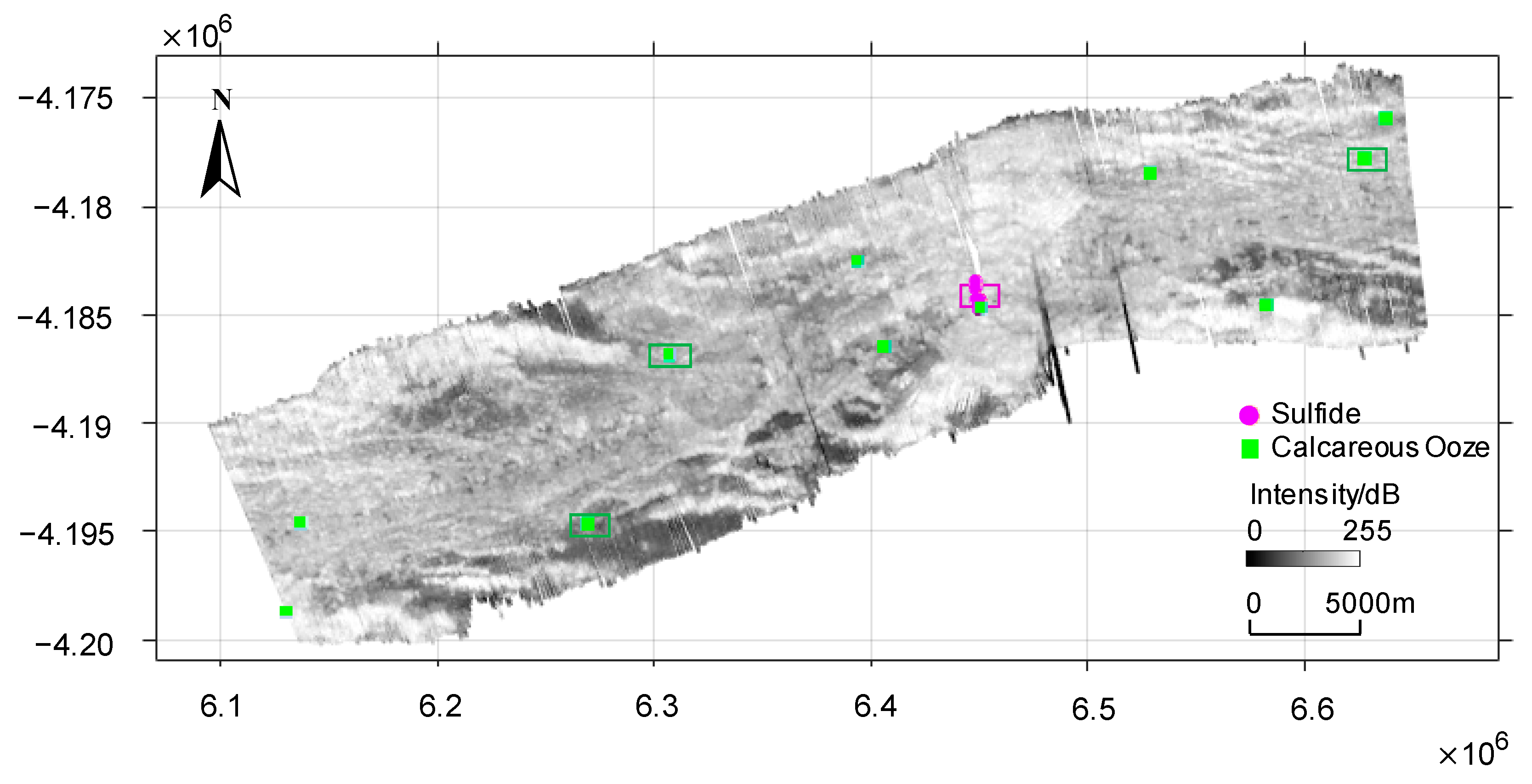
2.1. Overview of the Study Area

The mid-ridge of the Southwest Indian Ocean is approximately 8000 km long, starting from the Bouvet Triple Junction (BTJ, 55°S, 00°40′W) in the West and the Rodrigues Triple Junction (RTJ, 25°30′S, 70°E) in the East, which forms the boundary between the African and Antarctic Plates [30]. The West end of the Southwest Indian Ridge meets the Atlantic Ridge and America–Antarctica Ridge at the BTJ. At the Eastern end of the Southwest Indian Ridge, it meets the Central Indian Ridge and Southeast Indian Ridge at the RTJ. The expansion rate of the Indian Ocean ridge is 13–16 mm/a, which belongs to the ultraslow expansion mid-ocean ridge [31,32,33,34].
The Longqi hydrothermal area (37°47′S, 49°39′E) is the hydrothermal anomaly area discovered in the Southwest Indian Ridge in 2007, and it is the first area with hydrothermal activity discovered in the global ultraslow spreading oceanic ridge [31,32,33,34]. The water depth of the Longqi hydrothermal area is approximately 2100–3400 m. The Longqi hydrothermal point is located on a high hill at the Southeast end of the ridge valley at a depth of approximately 1755 m. The topography of the surrounding area significantly fluctuates; it is higher in the South and lower in the West. Overall, it has a steep slope, and basalt appears on the seabed with few surface sediments [31,32,33,34] (Figure 1).
An EM122 high-precision deep-water multibeam echo sounder system, which is produced by the Kongsberg company of Norway, is used in the topographic and geomorphological survey of the Southwest Indian Ridge. Its working frequency is 12 kHz, the depth measurement range is 20–11,000 m, the beam spacing is 1° × 1°, the number of beams is 288, and the coverage width is typically 6 times that of the water depth, to more than 30 km. EM 122 uses both CW and FM pulse forms, its effective pulse length is 1 ms CW to 100 ms FM. FM sweep with pulse compression on reception was used to increase the maximum useful swath width, as well as the resolution; the range sampling rate is 3.03 kHz (25 cm). The system was used to acquire a large amount of high-precision multibeam sonar data in the Longqi hydrothermal area of the Southwest Indian Ocean. Pushcore was used to acquire deep-sea sediment sampling data, providing a large amount of detailed data for the quantitative study of the topography and the distribution characteristics of surface sediments in the hydrothermal seabed area.

2.2. Fine Processing of Deep-Sea Multibeam Backscatter Intensity Data

The backscatter intensity represents the reflection and scattering abilities of seabed media. It depends on the incident angle of the sound waves, the roughness of the seabed, and the physical characteristics of the sediments.
The seabed backscatter intensity can be expressed as [36,37,38]:
B S = B S B + 10 log A
Here, B S B is the intrinsic scattering intensity of the seabed, which typically depends on the incident angle θ of the beam. A represents the area of the beam irradiation, which can be obtained from the propagation speed ( c ) of sound waves in water, pulse width ( τ ) , transmitting beam width ( θ T ) , receiving beam width (θR), and incident angle (θ) of beams. For different values of θ , A corresponds to different areas.
{ B S N + 10 log ( θ T θ R R 2 ) ( θ = 0 ° ) B S O + 10 l o g c o s 2 θ + 10 log c τ θ T R 2 sin θ ( θ 0 )
When θ = 0°, BSB is approximately equal to a constant BSN. When θ ≠ 0°, BSB depends on the incident angle of the beam and the characteristics of seabed sediment types, and its variation obeys Lambert’s law.
BSN and BSO are the backscatter intensities of seabed sediment at the normal and oblique incidence of sound waves, respectively. BSO only reflects the characteristics of seabed sediment types. The incident angle θ can be determined according to Snell’s law.
Because of the absorption of sound waves by the sea, the energy of sound decays with increasing distance, and the variation of the seabed topography will affect the size of the beam irradiation area, leading to the deviation of intensity calculation. The original multibeam backscatter intensity cannot directly reflect the real seabed sediment characteristics; it must be subjected to fine postprocessing [21]. The commonly used deep-sea multibeam backscatter intensity postprocessing algorithm does not consider the effects of deep-sea acoustic signal propagation loss, seabed topography fluctuation, and central beam specular reflection on backscatter intensity. In this study, the effects of deep-sea acoustic signal propagation loss and seabed topography fluctuation on backscatter intensity were analyzed. We used sediment classification software independently developed by the research group. Furthermore, this process included an existing multibeam backscatter intensity data correction model that was improved, in particular, by taking into consideration factors such as the influence of the seabed topography and the influence of reflected signals in the central beam area, and obtained the backscatter intensity value, which can truly reflect the characteristics of seabed sediments using a median filtering algorithm (Figure 2).

2.2.1. Compensation for Propagation Loss of Deep-Sea Acoustic Signal

The acoustic signal transmitted by the multibeam echo sounder system weakens as the propagation time increases because of the expansion loss and absorption by seawater and seabed sediments. The loss of backscatter intensity is more significant in deep-sea detection; thus, it is necessary to amplify and compensate the signal intensity according to the time variation. Thus, the original level of the echo signal is achieved and the effect of the marine environment on the sound wave intensity is weakened.
In the process of multibeam sonar data acquisition, the system maintains the acoustic signal within a certain dynamic range for automatic gain processing. However, due to different working environments, this automatic gain processing method produces a large error. In the fine processing of multibeam backscatter intensity data, it is necessary to remove the system gain. Then, the gain is recalculated and added to the correction process. The time variable gain (TVG) of an EM series multibeam is calculated as follows:
G L = x log R + 2 α R + c
where x and c are typically set as fixed parameters of 20, and R represents the transmission distance of sound waves. α represents the absorption coefficient, which is related to the emission frequency of sound waves, seawater temperature, and salinity, and is 29 dB/km at 100 kHz.
After calculating the system gain of a multibeam using Formula (3), the real echo intensity level was obtained using the receiving transducer before correction, which is convenient for correction according to the real-time marine environment state.
According to the sonar equation, the propagation loss related to the distance (time) can be obtained as follows:
G L r = 2 × n × 10 log R + 2 α R / 10 3
The coefficient n (=1.5) is related to the beam emission angle; the EM122 series multibeam system has a transmission frequency of 12 kHz; the absorption coefficient α is 6 dB/km; and R represents the transmission distance of sound waves.

2.2.2. Correction of the Influence of Deep-Sea Seabed Terrain Slope

In the Longqi hydrothermal area, the seabed topography is complex, and the water depth varies significantly. The seabed terrain slope significantly influences the intensity of multibeam backscatter. In addition, the terrain influence correction model is complex. To obtain an accurate terrain influence correction model, an accurate seabed digital terrain model (Figure 3) was constructed using finely processed high-precision multibeam bathymetric data. Then, the terrain slope influence correction calculation was performed for each backscatter intensity value.
Considering terrain slope correction, the actual incident angel θ’ of the multibeam is:
θ = arccos ( V i V n V i V n )
Vi represents the incident angle vector and Vn represents the normal vector perpendicular to the seabed.
Due to the influence of terrain slope, area A of the beam irradiation changes, affecting the calculation accuracy of backscatter intensity. Thus, it needs to be corrected.
The total influence of seabed terrain on echo intensity is as follows:
Δ B s = 10 l o g c τ ψ t R 2 s i n ( θ + β ) + 10 l o g c o s ( θ + β ) ( 10 l o g c τ ψ t R 2 sin ( θ ) + 10 l o g c o s ( θ ) )
Among them, c represents the sound velocity, τ represents the pulse width, ψ t represents the received beamwidth, and β represents the slope angle.
β = arccos ( | C | A 2 + B 2 + C 2 )
After multiple filtering, the least square method was used to fit the surface for five consecutive pings. Then, the normal vectors (A, B, and C) of each sampling point were obtained, thereby obtaining the accurate slope angle.

2.3. Fuzzy ISODATA Unsupervised Sediment Classification

2.3.1. Principle of Algorithm

The fuzzy ISODATA algorithm [39] was used to select the initial cluster center according to the preset number of clusters. Then, the fuzzy matrix U is compared according to the criterion function. At the same time, it merges and decomposes the categories not meeting the requirements until they are satisfied. The fuzzy ISODATA algorithm differs from the traditional K-means clustering algorithm [40], mainly by introducing U and incorporating the two mechanisms of merging and splitting in the iterative process. When the number of samples belonging to a certain category is too small, the category is removed. Conversely, when the number of samples belonging to a certain category is too large and scattered, the category is divided into two subcategories.
Assume that the number of sampling matrix X = { X 1 , X 2 , , X N } is N and each sampling point contains S-dimensional features. Define the cluster center Z = { Z 1 , Z 2 , , Z K } . The construction criterion function is defined as follows:
J = i = 1 K i = 1 K [ μ i j ( L + 1 ) ] m | X j Z i | 2
where μ i j means the matrix element of membership matrix U . L represents the number of iterations. Through repeated iterations of the matrix U and the clustering center Z , the criterion function J was minimized.

2.3.2. Algorithm Flow

The fuzzy ISODATA algorithm flow is as follows:
  • Input the initial parameters and randomly select the initial cluster center Z i (0).
  • Calculate the initial membership matrix U(0) according to Formula (8).
  • Through the initial membership matrix U(0), calculate all kinds of new cluster centers Z i (0).
  • Choose whether to perform the split operation.
  • Judge the merge operation. If the distance between the categories is less than the set threshold or the number of samples in a category is less than the specified number, then the merge operation will be performed.
  • According to the new clustering results, calculate the distance d between each sample and each clustering center.
  • Calculate a new membership matrix.
  • Return to step 3 and repeat the iteration until it completes.

2.4. Improved SVM Supervised Sediment Classification

2.4.1. Classification Method

SVM is a new machine learning method proposed by Vapnik [41,42] based on statistical theory and structural risk minimization criteria. It is used to solve classification and function approximation problems. SVM has a stricter theoretical and mathematical foundation and stronger generalization ability than traditional machine learning methods, such as backpropagation neural networks. It does not have a local minimum problem. It is suitable for small sample learning and can solve the problems of local minima, nonlinearity, over-learning, and dimension disaster [42]. It is widely used in complex data classification, signal processing, and regression function estimation [43,44]. However, in practice, because the problem of selecting optimal parameters of SVM has not been satisfactorily solved, the commonly used SVM parameter selection generally adopts the exhaustive method. This method has many disadvantages, such as large calculation, long operation time, low optimization precision, and difficulty in obtaining optimal parameters.
GA is an adaptive optimization technique proposed by Holland [45] that is based on genetics and evolutionary mechanisms and is suitable for complex system optimization. Compared with traditional optimization algorithms, GA optimization has the advantages of high search efficiency, global optimal solution search, avoidance of falling into a local optimal solution, no influence of objective functions, and strong adaptability.
In this study, to solve the problems of difficult parameter selection and low precision of SVM, GA is used to build a GA–SVM classification model. Based on high-precision multibeam sonar data obtained from the Longqi hydrothermal area in the Southwest Indian Ocean, the multidimensional seabed topography and seabed intensity information features of the Longqi hydrothermal area were extracted and input to the GA–SVM optimization classification model. The experimental results showed that the model could further improve the classification accuracy and speed of deep-sea seabed sediments.

2.4.2. GA-SVM Classification Model

The SVM classification model maps sample space to high-dimensional space and then constructs the optimal decision function in the high-dimensional feature space [46]:
y = w T · φ ( x ) + b
Here, w represents a weight vector and b. represents the offset.
The SVM model is used to solve classification problems through optimizations [42],
m i n 1 2 w 2 + C i = 1 n ε i   , s . t . , y i ( w x i + b ) 1 ε i , ε i > 0
Here, ε i represents the introduced relaxation variable, and C represents the penalty factor. The Lagrange multiplier is introduced for an optimal calculation to obtain the SVM decision function [45]:
f ( x ) = s i g n [ i = 1 n α i y i K ( x i , y i ) + b ]
The value of the penalty factor C in the SVM classification model and the RBF parameter g directly affect the accuracy of SVM classification. In particular, C is proportional to the fitting degree of data. The larger the value of C , the higher the degree of data fitting. The RBF parameter g , i.e., linear indivisibility, is determined. g that is excessively large after the sample data are mapped to the high-dimensional feature space reduces the classification accuracy. Therefore, a reasonable selection of parameters is essential to ensure and improve the classification performance of SVM.
GA has a strong robustness and global optimization ability. Its greatest advantage is that only the objective function (fitness function) is used in the optimization process instead of the gradient and other auxiliary information. Its optimization process starts from the solution space point set to the global optimum. With this feature, we can choose the best optimization parameters for SVM, thereby improving the convergence speed and classification accuracy of the network. The specific optimization process is shown in Figure 4.

2.4.3. Feature Extraction

We extracted 24-dimensional feature information, including topographic factors and texture features, from the seabed topographic and sound intensity data obtained from the Longqi hydrothermal area in the Southwest Indian Ridge, as shown in Table 1.
R5, L5, E5, S5, and W5 constitute a one-dimensional vector set with a length of 5. They represent grayscale, edge, point, wave, and ripple characteristics, respectively, which are defined as follows:
{ L 5 = [ 1   4   6   4   1 ] E 5 = [ 1 2   0   2   1 ] S 5 = [ 1   0   2   0 1 ] W 5 = [ 1   2   0 2   1 ] R 5 = [ 1 4   6 4   1 ]
S5R5, L5R5, L5S5, E5S5, E5W5, S5W5 are obtained by the convolution of the corresponding texture vector.

3. Results

3.1. Processed Results of Deep-Sea Multibeam Backscatter Intensity Data

3.1.1. Results of Compensation for Propagation Loss of Deep-Sea Acoustic Signal

In the Formula (4), n and α can be adjusted during data processing to obtain the best sonar image. As shown in Figure 5, after the acoustic signal is corrected, and most of the outliers of sound intensity are effectively eliminated. In the red square area of the Figure 5b,c, the intensity changes are balanced, and the intensity value of noise is restored to a normal magnitude after TVG correction. The image darkening caused by transmission loss is improved, and the intensity value of the abnormal bulge is reduced (Figure 5).

3.1.2. Results of Correction of the Influence of Deep-Sea Seabed Terrain Slope

The actual beam irradiation area A’ was calculated using Formulas (6) and (7). The seabed terrain slope and beam irradiation area were corrected using Formula (1). Finally, the BS, which is independent of the incident angle and only reflects the characteristics of the deep seabed, was obtained. As shown in Figure 6a, green and blue represent the sound intensity data corrected by TVG and the terrain slope, respectively. The abnormal mutation of the original sound intensity data is eliminated and the corrected sound intensity changes smoothly, preserving the intensity characteristic information. By correcting the effect of propagation loss and the seabed terrain slope, the image details in different areas were preserved, the influence of the intensity change was weakened, and the speckle noise in the image was removed by median filtering. We obtained backscatter intensity data reflecting real seabed sediment characteristics to generate sonar images (Figure 6b,c). The details of the image are clear, the transition of the survey line is natural, and the bright band in the central area was successfully removed. The trend characteristics of the backscatter intensity changing with the incident angle can be observed. However, when they are combined with the sound intensity variation graph, information about seabed sediments in the strip coverage area can be visually described. Thus, the types of seabed sediments can be accurately and quantitatively analyzed.

3.2. Deep-Sea Sediment Classification Results Using Fuzzy ISODATA Unsupervised

Four areas were selected as the test data of the fuzzy ISODATA classification algorithm from the seabed sediment sampling data collected in the Longqi hydrothermal area in the third leg of Dayang 52 voyage (Figure 1) and the sediment sampling data collected in this area through the census of seafloor sediments in the world’s ocean [52]. One of these is sulfide and has a total of 9000 samples (as shown in the purple box in Figure 7). There are 9000 samples in 3 calcareous ooze sediment areas (as shown in the green box in Figure 7).
The fuzzy ISODATA algorithm was used to obtain the distribution of seabed sediment types in the Longqi hydrothermal area in the Southwest Indian Ridge (Figure 8).

3.3. Deep-Sea Sediment Classificaiton Results Using Improved SVM Supervised Sediment Classification

To verify the effectiveness of the GA–SVM classification model in classifying deep-seabed sediments, two types of seabed sediments—sulfide and calcareous ooze—were selected in the Longqi hydrothermal area in the Southwest Indian Ridge (Figure 7). In total, 9000 sulfide samples (4500 training and test samples) and 9000 calcareous ooze samples (4500 training and test samples) were collected.
Training data were input into the SVM and GA–SVM classification models for training and learning, respectively. Then, the models were tested with the test data. Finally, the entire Longqi hydrothermal area was classified by sediment; the classification results of the two classifiers are shown in Figure 9.

4. Discussion

Previous studies mainly focused on acoustic sediment classification in shallow seas. This study achieves the automatic identification and classification of deep-seabed sediment types using an acoustic remote sensing method, which has important theoretical and practical significance for deep-sea resource investigation, deep-sea marine engineering applications, and deep-sea marine scientific research.
First, the unsupervised fast classification of deep-seabed sediment was realized using the fuzzy ISODATA algorithm, and the overall classification accuracy and Kappa coefficient were calculated according to Formulas (13)–(15) [53,54].
Overall = x i i N
kappa   = Overall p e 1 p e
p e = i = 1 n ( j = 1 n x i j + i = 1 n x j i ) N 2
where, x i i is the number of correctly classified, N is the total number of samples, j = 1 n x i j is the sum of the i-th row, and i = 1 n x j i is the sum of the i-th column elements.
As shown in Figure 8, unsupervised classification does not require an in-depth understanding of the image to be classified in advance. It can quickly classify the types according to the set types. However, compared with supervised classification, its classification accuracy is lower (shown in Table 2). In addition, because the input data is unlabeled, unsupervised classification has no definite result. The fuzzy ISODATA unsupervised classification is mainly used to roughly classify sediment types without on-site geological sampling.
Second, combining GA with the SVM neural network can rapidly and efficiently identify deep-sea sulfide, deep-sea calcareous ooze, and other sediment types. Figure 9 and Table 3 show that the classification accuracy of the GA-SVM model is higher than that of the SVM neural network, achieving up to 89.10% and 89.66% classification accuracy for deep-sea sulfide and calcareous ooze, respectively. Based on experimental comparison and analysis results, the classification accuracy of the GA-SVM model is significantly higher than that of the SVM model, and the overall accuracy reaches 89.66%. It can be effectively applied to high-precision deep-sea sediment classification and recognition.
Due to the lack of more sampling data of different types of sediment in the Longqi hydrothermal area, our multibeam acoustic sediment classification test has certain limitations. In future research, we will collect more sediment sampling data in deep water areas and extend the acoustic sediment classification method to identify various types of seabed sediments.

5. Conclusions

In this study, the EM122 multibeam sonar data collected in the Longqi hydrothermal area in the Southwest Indian Ridge, in April 2019 were used to analyze multibeam backscatter intensity data considering various errors in the complex deep-sea environment. Thus, backscatter intensity data truly reflecting the seabed sediment types were obtained. Through unsupervised and supervised classification, the classification of seabed sediments in the Longqi hydrothermal area was studied. The results showed that the accuracy of supervised classification is higher than that of unsupervised classification. Unsupervised classification is mainly used to roughly classify sediment types without on-site geological sampling. The classification accuracy of the GA-SVM algorithm is better than that of the traditional SVM algorithm and ISODATA algorithm. However, due to parameter iterative optimization and training, it takes longer than the other two methods. When there is enough sampling data, the GA-SVM algorithm is recommended.
Through this research work, we can provide accurate seabed topography and sediment data for the exploration of deep-sea hydrothermal resources and the assessment of benthic habitats in deep-sea hydrothermal areas, thereby contributing to a comprehensive understanding of the impact of human activities on the deep-sea environment.

Author Contributions

Conceptualization, Q.T.; methodology, Q.T.; software, D.D. and X.J.; validation, Q.T. and J.L.; formal analysis, Q.T.; investigation, L.Y. and W.S.; data curation, Q.T. and J.L.; writing–original draft preparation, Q.T., J.L., D.D. and X.J.; writing–review and editing, J.L. and N.L.; visualization, D.D. and N.L.; supervision, Q.T. and J.L.; project administration, Q.T.; funding acquisition, Q.T. All authors have read and agreed to the published version of the manuscript.

Funding

This work was supported by the National Natural Science Foundation of China (41876111), the National Key R&D Program of China (2018YFC0309901), and the Key Laboratory of Ocean Geomatics, Ministry of Natural Resources, China (Grant No. 2021B04).

Data Availability Statement

The datasets generated during the current study are not publicly available due to data not being public but are available from the corresponding author upon reasonable request.

Acknowledgments

We thank the captain and crew of the R/V Dayangyihao during the third leg of the COMRA DY52nd cruise, as well as for the EM122 sonar data and seabed sediment samples data obtained on this cruise.

Conflicts of Interest

The authors declare no conflict of interest.

References

  1. Urick, R.J. Principles of Underwater Sounder, 3rd ed.; McGraw-Hill: New York, NY, USA, 1983. [Google Scholar]
  2. Anderson, J.T.; Holliday, D.V.; Kloser, R.; Reid, D.G.; Simard, Y. Acoustic seabed classification: Current practice and future directions. ICES J. Mar. Sci. 2008, 65, 1004–1011. [Google Scholar] [CrossRef]
  3. Reut, Z.; Pace, N.G.; Heaton, M.J.P. Computer classification of sea beds by sonar. Nature 1985, 314, 426–428. [Google Scholar] [CrossRef]
  4. Pace, N.G.; Gao, H. Swathe seabed classification. IEEE J. Ocean. Eng. 1988, 13, 83–90. [Google Scholar] [CrossRef]
  5. Subramaniam, S.; Barad, H.; Martinez, A.B.; Bourgeois, B. Seafloor characterization using texture. In Proceedings of the IEEE Southeastcon’93, Charlotte, NC, USA, 4–7 April 1993; Volume 93, pp. 299–317. [Google Scholar]
  6. Mitchell, N.C.; Hughes Clarke, J.E. Classification of seafloor geology using multibeam sonar data from the Scotian Shelf. Mar. Geol. 1994, 121, 143–160. [Google Scholar] [CrossRef]
  7. Pican, N.; Trucco, E.; Ross, M.; Lane, D.M.; Petillot, Y.; Tena Ruiz, I. Texture analysis for seabed classification: Co-occurrence matrices vs. self-organizing maps. In Proceedings of the IEEE OCEANS’98, Nice, France, 28 September–1 October 1998; Volume 1, pp. 424–428. [Google Scholar]
  8. Blondel, P.; Gómez Sichi, O. Textural analyses of multibeam sonar imagery from Stanton Banks, Northern Ireland continental shelf. Appl. Acoust. 2009, 70, 1288–1297. [Google Scholar] [CrossRef]
  9. Huseby, R.B.; Milvang, O.; Solberg, A.S.; Bjerde, K.W. Seabed classification from multibeam echosounder data using statistical methods. In Proceedings of the IEEE OCEANS’93, Victoria, BC, Canada, 18–21 October 1993; Volume 3, pp. 229–233. [Google Scholar]
  10. Alevizos, E.; Snellen, M.; Simons, D.G.; Siemes, K.; Greinert, J. Acoustic discrimination of relatively homogeneous fine sediments using Bayesian classification on MBES data. Mar. Geol. 2015, 370, 31–42. [Google Scholar] [CrossRef]
  11. Simons, D.G.; Snellen, M. A Bayesian approach to seafloor classification using multi-beam echo-sounder backscatter data. Appl. Acoust. 2009, 70, 1258–1268. [Google Scholar] [CrossRef]
  12. Lucieer, V.; Lucieer, A. Fuzzy clustering for seafloor classification. Mar. Geol. 2009, 264, 230–241. [Google Scholar] [CrossRef]
  13. Menandro, P.S.; Bastos, A.C.; Boni, G.; Ferreira, L.C.; Vieira, F.V.; Lavagnino, A.C.; Moura, R.L.; Diesing, M. Reef Mapping Using Different Seabed Automatic Classification Tools. Geosciences 2020, 10, 72. [Google Scholar] [CrossRef] [Green Version]
  14. Janowski, L.; Kubacka, M.; Pydyn, A.; Popek, M.; Gajewski, L. From acoustics to underwater archaeology: Deep investigation of a shallow lake using high-resolution hydroacoustics-The case of Lake Lednica, Poland. Archaeometry 2021, 63, 1059–1080. [Google Scholar] [CrossRef]
  15. Misiuk, B.; Lecours, V.; Dolan, M.F.; Robert, K. Evaluating the Suitability of Multi-Scale Terrain Attribute Calculation Approaches for Seabed Mapping Applications. Mar. Geod. 2021, 44, 327–385. [Google Scholar] [CrossRef]
  16. Alexandrou, D.; Pantzartzis, D. Seafloor classification with neural networks. In Proceedings of the Engineering in the Ocean Environment, Washington, DC, USA, 24–26 September 1990; pp. 18–23. [Google Scholar]
  17. Kavli, T.; Carlin, M.; Madsen, R. Seabed classification using artificial neural networks and other nonparametric methods. In Proceedings of the International Conference on Acoustic Classification and Mapping of the Seabed, Bath, UK, 15–17 December 1993; pp. 141–148. [Google Scholar]
  18. Michalopoulou, Z.H.; Alexandrou, D.; de Moustier, C. Application of neural and statistical classifiers to the problem of seafloor characterization. IEEE J. Ocean. Eng. 1995, 20, 190–197. [Google Scholar] [CrossRef]
  19. Chakraborty, B.; Kaustubha, R.; Hegde, A.; Pereira, A. Acoustic seafloor sediment classification using self-organizing feature maps. IEEE Trans. Geosci. Remote Sens. 2001, 39, 2722–2725. [Google Scholar] [CrossRef]
  20. Ojeda, G.Y.; Gayes, P.T.; Van Dolah, R.F.; Schwab, W.C. Spatially quantitative seafloor habitat mapping: Example from the northern South Carolina inner continental shelf. Estuarine. Coast. Shelf Sci. 2004, 59, 399–416. [Google Scholar] [CrossRef]
  21. Tang, Q.H.; Lei, N.; Li, J.; Wu, Y.T.; Zhou, X.H. Seabed mixed sediment classification with multibeam echo sounder backscatter data in Jiaozhou Bay. Mar. Georesour. Geotechnol. 2015, 33, 1–11. [Google Scholar] [CrossRef]
  22. Ji, X.; Yang, B.S.; Tang, Q.H. Seabed sediment classification using multibeam backscatter data based on the selecting optimal random forest model. Appl. Acoust. 2020, 167, 107387. [Google Scholar] [CrossRef]
  23. Tang, Q.H.; Liu, X.Y.; Ji, X.; Li, J.; Chen, Y.L.; Lu, B. Using seabed acoustic imagery to characterize and classify seabed sediment types in the pockmark area of the North Yellow Sea, China. Appl. Acoust. 2021, 174, 107748. [Google Scholar] [CrossRef]
  24. Ji, X.; Yang, B.S.; Tang, Q.H. Acoustic seabed classification based on multibeam echosounder backscatter data using the PSO-BP-AdaBoost algorithm: A case study from Jiaozhou Bay, China. IEEE J. Ocean. Eng. 2021, 46, 509–519. [Google Scholar] [CrossRef]
  25. Zhang, K.; Li, Q.; Zhu, H.; Yang, F.; Wu, Z. Acoustic Deep-Sea Seafloor Characterization Accounting for Heterogeneity Effect. IEEE Trans. Geosci. Remote Sens. 2020, 58, 3034–3042. [Google Scholar] [CrossRef]
  26. Cui, X.D.; Yang, F.L.; Wang, X.; Ai, B.; Luo, Y.; Ma, D. Deep learning model for seabed sediment classification based on fuzzy ranking feature optimization. Mar. Geol. 2021, 432, 106390. [Google Scholar] [CrossRef]
  27. Halpern, B.S.; Walbridge, S.; Selkoe, K.A.; Kappel, C.V.; Micheli, F.; D’Agrosa, C.; Bruno, J.F.; Casey, K.S.; Ebert, C.M.; Fox, H.E.; et al. A Global Map of Human Impact on Marine Ecosystems. Science 2008, 319, 948–952. [Google Scholar] [CrossRef] [PubMed] [Green Version]
  28. Halpern, B.S.; Frazier, M.; Potapenko, J.; Casey, K.S.; Koenig, K.; Longo, C.; Lowndes, J.S.; Rockwood, R.C.; Selig, E.R.; Selkoe, K.A.; et al. Spatial and temporal changes in cumulative human impacts on the world’s ocean. Nat. Commun. 2015, 6, 7615. [Google Scholar] [CrossRef] [PubMed] [Green Version]
  29. Madricardo, F.; Foglini, F.; Campiani, E.; Grande, V.; Catenacci, E.; Petrizzo, A.; Kruss, A.; Toso, C.; Trincardi, F. Assessing the human footprint on the sea-floor of coastal systems: The case of the Venice Lagoon, Italy. Sci. Rep. 2019, 9, 6615. [Google Scholar] [CrossRef] [PubMed]
  30. Van Dover, C.L.; Humphris, S.E.; Fornari, D.; Cavanaugh, C.M.; Collier, R.; Goffredi, S.K.; Hashimoto, J.; Lilley, M.D.; Reysenbach, A.L.; Shank, T.M.; et al. Biogeography and ecological setting of Indian Ocean hydrothermal vents. Science 2001, 294, 818–823. [Google Scholar] [CrossRef] [PubMed] [Green Version]
  31. Tao, C.H.; Lin, J.; Guo, S.Q.; John Chen, Y.S.; Wu, G.H.; Han, X.Q.; German, C.R.; Yoerger, D.R.; Zhou, N.; Li, H.M.; et al. The DY115–19 (Legs 1–2) and DY115–20 (Legs 4–7) Science Parties, First active hydrothermal vents on an ultraslow-spreading center: Southwest Indian Ridge. Geology 2012, 40, 47–50. [Google Scholar] [CrossRef]
  32. Tao, C.H.; Li, H.M.; Jin, X.B.; Zhou, J.P.; Wu, T.; He, Y.H.; Deng, X.M.; Gu, C.H.; Zhang, G.Y.; Liu, W.Y. Seafloor hydrothermal activity and polymetallic sulfide exploration on the southwest Indian ridge. Chin. Sci. Bull. 2014, 59, 2266–2276. [Google Scholar] [CrossRef]
  33. Tao, C.; Wu, T.; Liu, C.; Li, H.; Zhang, J. Fault inference and boundary recognition based on near-bottom magnetic data in the Longqi hydrothermal field. Mar. Geophys. Res. 2017, 38, 17–25. [Google Scholar] [CrossRef]
  34. Tao, C.H.; Seyfried, W.E.; Lowell, R.P.; Liu, Y.L.; Liang, J.; Guo, Z.K.; Ding, K.; Zhang, H.T.; Liu, J.; Qiu, L.; et al. Deep high-temperature hydrothermal circulation in a detachment faulting system on the ultra-slow spreading ridge. Nat. Commun. 2020, 11, 1300. [Google Scholar] [CrossRef] [Green Version]
  35. GEBCO Compilation Group (2021) GEBCO 2021 Grid (doi:10.5285/c6612cbe-50b3-0cff-e053-6c86abc09f8f). Available online: https://www.bodc.ac.uk/data/published_data_library/catalogue/10.5285/c6612cbe-50b3-0cff-e053-6c86abc09f8f/ (accessed on 28 March 2022).
  36. Lurton, X.; Dugelay, S.; Augustin, J.M. Analysis of multibeam echo-sounder signals from the deep seafloor. In Proceedings of the IEEE OCEANS’94, Brest, France, 13–16 September 1994; Volume 3, pp. 213–218. [Google Scholar]
  37. Zietz, S.; Satriano, J.H.; Geneva, A. Development of physically-based ocean bottom classification analysis system using multibeam sonar backscatter. In Proceedings of the IEEE OCEANS’96, Fort Lauderdale, FL, USA, 23–26 September 1996; Volume 3, pp. 1058–1063. [Google Scholar]
  38. Gonidec, Y.L.; Lamarche, G.; Wright, I.C. Inhomogeneous substrate analysis using EM300 backscatter imagery. Mar. Geophys. Res. 2003, 24, 311–327. [Google Scholar] [CrossRef]
  39. Bezdek, J.C. A convergence theorem for the fuzzy ISODATA clustering algorithms. IEEE Trans. Pattern Anal. Mach. Intell. 1980, PAMI-2, 1–8. [Google Scholar] [CrossRef]
  40. MacQueen, J. Some methods for classification and analysis of multivariate observations. In Proceedings of the 5th Berkeley Symposium on Mathematical Statistics and Probability; Berkeley, University of California Press: Oakland, CA, USA, 1967; pp. 281–297. [Google Scholar]
  41. Vapnik, V.N. The Nature of Statistical Learning Theory; Springer: Berlin/Heidelberg, Germany, 1995. [Google Scholar]
  42. Vapnik, V.N. An overview of statistical learning theory. IEEE Trans. Neural Netw. 1999, 10, 988–999. [Google Scholar] [CrossRef] [PubMed] [Green Version]
  43. Burges, C. A tutorial on support vector machines for pattern recognition. Data Min. Knowl. Discov. 1998, 2, 121–167. [Google Scholar] [CrossRef]
  44. Smola, A.J.; Schölkopf, B. A tutorial on support vector regression. Stat. Comput. 2004, 14, 199–222. [Google Scholar] [CrossRef] [Green Version]
  45. Holland, J.H. Adaptation in Natural and Artificial System; The University of Michigan Press: Ann Arbor, MI, USA, 1975; pp. 12–27. [Google Scholar]
  46. Yu, E.; Cho, S. GA-SVM wrapper approach for feature subset selection in keystroke dynamics identity verification. In Proceedings of the International Joint Conference on Neural Networks, Portland, OR, USA, 20–24 July 2003; Volume 3, pp. 2253–2257. [Google Scholar]
  47. Moya, E.; Neto, A.A. Side scan sonar images attributes characterization for seabed mapping. In Proceedings of the 2015 IEEE/OES Acoustics in Underwater Geosciences Symposium (RIO Acoustics), Rio de Janeiro, Brazil, 29–31 July 2015; pp. 1–4. [Google Scholar]
  48. Mougiakakou, S.G.R.; Golemati, S.; Gousias, I.; Nicolaides, A.N.; Nikita, K.S. Computer-aided diagnosis of carotid atherosclerosis based on ultrasound image statistics, laws’ texture and neural networks. Ultrasound Med. Biol. 2007, 33, 26–36. [Google Scholar] [CrossRef]
  49. Manjunath, B.S.; Ma, W.Y. Texture features for browsing and retrieval of image data. IEEE Trans. Pattern Anal. Mach. Intell. 1996, 18, 837–842. [Google Scholar] [CrossRef] [Green Version]
  50. Howarth, P.; Rüger, S. Evaluation of texture features for content-based image retrieval. In International Conference on Image and Video Retrieval; Springer: Berlin/Heidelberg, Germany, 2004; pp. 326–334. [Google Scholar]
  51. Ojala, T.; Pietikainen, M.; Maenpaa, T. Multiresolution gray-scale and rotation invariant texture classification with local binary patterns. IEEE Trans. Pattern Anal. Mach. Intell. 2002, 24, 971–987. [Google Scholar] [CrossRef]
  52. Dutkiewicz, A.; Müller, R.D.; O’Callaghan, S.; Jónasson, H. Census of seafloor sediments in the world’s ocean. Geology 2015, 43, 795–798. [Google Scholar] [CrossRef]
  53. Diesing, M.; Mitchell, P.J.; O’Keeffe, E.; Gavazzi, G.; Bas, T.L. Limitations of predicting substrate classes on a sedimentary complex but morphologically simple seabed. Remote Sens. 2020, 12, 3398. [Google Scholar] [CrossRef]
  54. Pontius, R.G., Jr.; Millones, M. Death to kappa: Birth of quantity disagreement and allocation disagreement for accuracy assessment. Int. J. Remote Sens. 2011, 32, 4407–4429. [Google Scholar] [CrossRef]
Figure 1. Schematic location of Longqi hydrothermal area (The basemap elevation data comes from the GEBCO [35]).
Remotesensing 14 02675 g001
Figure 2. Fine processing flowchart of deep-sea multibeam backscatter intensity data.
Remotesensing 14 02675 g002
Figure 3. High-precision seabed DTM (100 m × 100 m grid) in the Longqi hydrothermal area.
Remotesensing 14 02675 g003
Figure 4. Flowchart of GA-SVM neural network calculation.
Remotesensing 14 02675 g004
Figure 5. Influence of propagation loss on backscatter intensity: (a) correction intensity diagram of acoustic signal propagation loss; (b) original sonar image without TVG correction; and (c) seabed sonar image after TVG correction.
Remotesensing 14 02675 g005
Figure 6. Influence of seabed topography fluctuation on backscatter intensity and corrected intensity image in the Longqi hydrothermal area: (a) sound intensity contrast chart after TVG correction and terrain slope correction; (b) original sonar image without terrain slope correction; and (c) seabed sonar image after terrain slope correction.
Remotesensing 14 02675 g006aRemotesensing 14 02675 g006b
Figure 7. Location and type distribution of seabed geological sampling points in Longqi hydrothermal area.
Remotesensing 14 02675 g007
Figure 8. Seabed sediment classification results using unsupervised Fuzzy ISODATA.
Remotesensing 14 02675 g008
Figure 9. Results of seabed sediment classification by supervised SVM and GA–SVM: (a) seabed sediment classification results using SVM; and (b) seabed sediment classification results using GA–SVM.
Remotesensing 14 02675 g009aRemotesensing 14 02675 g009b
Table 1. Statistical table of 24-dimensional characteristic information.
NumberCharacteristicsDescriptionNumberCharacteristicsDescription
1GrayIntensity value13GLCM [47]Correlation
2DepthDepth14 Contrast
3Terrain factorSlope15 Variance
4 Curvature16 Inverse different moment
5Laws [48]Laws microscopic filter operator-L5R517 Mean
6 Laws microscopic filter operator- L 5 S 5 18 Dissimilarity
7 Laws microscopic filter operator- E 5 S 5 19Gabor [49]
8 Laws microscopic filter operator- E 5 W 5 20 45°
9 Laws microscopic filter operator- S 5 W 5 21 90°
10 Laws microscopic filter operator- S 5 R 5 22Tamura [50]Contrast
11GLCM [47]Energy23 Roughness
12 Entropy24LBP [51]Local binary pattern feature
Table 2. Classification accuracy of fuzzy ISODATA unsupervised sediment.
MethodClassification Accuracy (%)Overall (%)Kappa
ISODATASulfide/83.47
Calcareous ooze/85.43
85.450.689
Table 3. Classification accuracy of SVM and GA-SVM.
MethodClassification Accuracy (%)Overall (%)Kappa
SVMSulfide/84.81
Calcareous ooze/86.10
85.460.7091
GA-SVMSulfide/89.10
Calcareous ooze/89.66
89.660.7932
Publisher’s Note: MDPI stays neutral with regard to jurisdictional claims in published maps and institutional affiliations.

