Article

Mapping the Levels of Soil Salination and Alkalization by Integrating Machining Learning Methods and Soil-Forming Factors

1
College of Land Science and Technology, China Agricultural University, Beijing 100193, China
2
Key Laboratory of Agricultural Land Quality, Ministry of Natural Resources, Beijing 100193, China
3
Institute of Agricultural Remote Sensing and Information Technology Application, Zhejiang University, Hangzhou 310058, China
4
College of Plant Science, Tarim University, Alar 843300, China
5
State Key Laboratory of Resources and Environmental Information System, Beijing 100101, China
*
Author to whom correspondence should be addressed.
These authors contributed equally to this work.
Remote Sens. 2022, 14(13), 3020; https://0-doi-org.brum.beds.ac.uk/10.3390/rs14133020
Submission received: 11 May 2022 / Revised: 11 June 2022 / Accepted: 20 June 2022 / Published: 23 June 2022
(This article belongs to the Special Issue Remote Sensing of Soil Salinity: Detection and Quantification)

Abstract

:
Accurate updating of soil salination and alkalization maps based on remote sensing images and machining learning methods plays an essential role in food security, biodiversity, and desertification. However, there is still a lack of research on using machine learning, especially one-dimensional convolutional neural networks (CNN)s, and soil-forming factors to classify the salinization and alkalization degree. As a case study, the study estimated the soil salination and alkalization by Random forests (RF) and CNN based on the 88 observations and 16 environmental covariates in Da’an city, China. The results show that: the RF model (accuracy = 0.67, precision = 0.67 for soil salination) with the synthetic minority oversampling technique performed better than CNN. Salinity and vegetation spectral indexes played the most crucial roles in soil salinization and alkalinization estimation in Songnen Plain. The spatial distribution derived from the RF model shows that from the 1980s to 2021, soil salinization and alkalization areas increased at an annual rate of 1.40% and 0.86%, respectively, and the size of very high salinization and alkalization was expanding. The degree and change rate of soil salinization and alkalization under various land-use types followed mash > salinate soil > grassland > dry land and forest. This study provides a reference for rapid mapping, evaluating, and managing soil salinization and alkalization in arid areas.

1. Introduction

Soil salinity (including soil salinization and alkalization) is a process of water-soluble salts accumulating on the soil surface layer. The saline soil with many salt ions and alkali ions prevents plant cells from absorbing water. The salt and alkali ions become toxic ions when they exceed a threshold level, seriously harming plant growth [1]. Hence, the process profoundly impacts sustainable agricultural development and food security [2,3]. Soil salinization is more likely to occur in areas with low relief and high underground water, intensive evaporation and light rainfall, and human interference. Especially, diverse land-use patterns significantly impact soil salt migration and accumulation. Food and Agriculture Organization of the United Nations reported that the area of soil salinization accounts for 8.7% of the earth’s continental area (https://www.fao.org/, accessed on 1 April 2022) and is increasing [4]. Various practices have been proposed to slow or even reverse the process of accumulating water-soluble salts to reduce soil salinization’s effects on the ecological environment and food security [5,6]. These practices require rapid and accurate mapping [7].
Traditional mapping, characterized as time-consuming, expensive, and laborious, could not provide real-time information for improving and preventing soil salinization. Contrary to the traditional mapping, digital soil mapping (DSM) can quickly obtain real-time and high-resolution spatial distribution and even spatiotemporal change information of soil salt at a large scale [8]. The principle of DSM for soil salinity is to build models between dependent variables (soil salinity) and soil formation factors, including topography, biology, climate, parent material, time, spatial location, and soil itself [9]. Thus, DSM provides a scheme for updating soil salinization information in real time.
Recently, many studies have reported that the application of remote sensing data (such as MODIS, Landsat, and Sentinel) in soil salt monitoring is a current and future research hotspot [8,10,11]. The coarse resolution of MODIS images limited their application. Compared with Landsat, the Sentinel-2 images have a higher spatial resolution (10 m) in the red, blue, green, and near-infrared spectrum. These bands can be combined and calculated to obtain various salinity and vegetation spectral indices, including salinity indices II (SI2) [12], normalized vegetation index (NDVI) [13], and canopy response salinity index (CRSI) [14]. Previous studies have revealed that Sentinel-2 combined with machine learning methods can further mine the correlation between dependent variables and remote sensing images [15,16,17,18]. Most of these studies found that random forest (RF) with Sentinel-2 MSI presented a good performance for soil salt prediction. Wang et al. (2020) compared four models with Sentinel-2 MSI bands and found that the RF model performs better than the Convolutional Neural Network (CNN) [16]. Recently, the CNN model with remote sensing images has gradually been used in soil properties prediction [19,20,21]. However, few studies have applied the one-dimensional CNN model in soil salt classification. The research that uses machine learning, especially one-dimensional CNN with soil-forming factors to classify salinity and alkalinity, is still lacking.
The study transforms the continuous data into the classification data according to the classification standard of salinization, which reduced the calculation and simplified the scheme. The overall goal of the research was to estimate and analyze the classification and causes of soil salination and alkalization by RF and CNN. The study’s specific objectives include: (1) evaluating the performance of RF and CNN in the classification of soil salination and alkalization. (2) Describe the spatial distribution of soil salination and alkalization derived from the best model and analyze the influencing factors. (3) Quantify the temporal variation in soil salination and alkalization and discuss the effects of land-use types on the change.

2. Materials and Methods
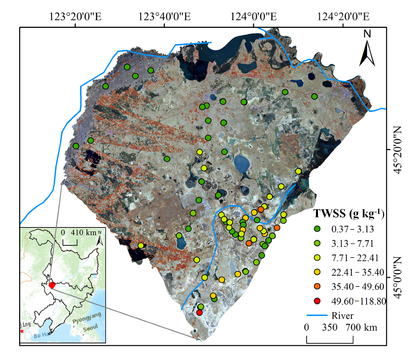
2.1. Study Area

The study area is located in Da’an city, Jilin Province, China, between 123°08′45″–124°21′56″E and 44°57′00″–45°45′51″N (Figure 1). It covers a total area of 487,900 hm2 and is a part of the Songnen basin. The average elevation is 120–160 m. The climate is temperate continental monsoon type with an average annual rainfall of 413.7 mm, an average annual temperature of 4.3 °C, and average annual evaporation of 1756.9 mm. Tao er, Nenjiang, and Huolin rivers are in the study area’s northwest, northeast, and central parts, respectively. According to the World Reference Base for Soil Resources, the soil is developed on the loess sediments and is characterized by four dominant soil types: Chernozem, Cambisol, Solonetz, and Solonchaks. Due to the flat terrain, light rainfall, intense evaporation, shallow groundwater, and human factors, salinization with carbonate as the dominant salt mineral has been noted in many areas in Da’an. In addition, bubble marsh is scattered all over the place. The study area is located in one of the world’s three largest soda saline soil regions and is a reserve food resource in China. Hence, choosing this region as the study area is representative and significant.

2.2. Data

2.2.1. Soil Sampling and Soil Analysis

The soil survey and sampling were conducted from 16 May 2021 to 25 May 2021. The sampling scheme considered the land-use type, salinization degree, and accessibility of sampling sites. Under this sampling scheme, a total of 88 topsoil samples (0–5 cm) were randomly selected. At each sampling site, a portion of 2 kg soil was collected and labeled. The geographical coordinates of each sample were recorded. After being air-dried, grounded, and passed through a 2 mm mesh, the soil was analyzed in the laboratory. The total water-soluble salt (TWSS), calcium ion (Ca2+), magnesium ion (Mg2+), sodium ion (Na+), potassium ion (K+), carbonate ion (CO32−), bicarbonate ion (HCO3), sulfate ion (SO42−), chloride ion (Cl), and pH were determined according to the conventional soil physical and chemical analysis methods. TWSS was measured by residue drying method, Ca2+, Mg2+, and SO42− were determined by EDTA complexometric titration method, and Na+ and K+ were determined by flame photometry. Soil suspension with a soil–water ratio of 1:5 was used to determine soil pH by electric potential method, CO32− and HCO3 were determined by double indicator neutralization titration, and Cl was determined by silver nitrate titration. The soil salination and alkalization classification in the 1980s was derived from the exchangeable sodium percentage (ESP) (%) and topsoil salinity (ECE) (Ds/m) data in the Harmonized World Soil Database [22].

2.2.2. Environmental Covariates

Table 1 shows the environmental factors, including terrain, vegetation, soil self, and climate data. Shuttle Radar Topography Mission (SRTM) provides a digital elevation model (DEM) with a 30 m spatial resolution. Other terrain factors, including curvature, valley depth (Vdepth), negative openness (Openn), topographic wetness index (TWI), and multi-resolution valley bottom flatness (MrVBF), were calculated from DEM through SAGA GIS [23].
The study used the Google Earth Engine (GEE) platform to obtain and process the Sentinel-2–MSI data. The Sentinel-2–MSI data was launched by the European Space Agency (ESA) and provided by the Copernicus Open Access Hub (https://scihub.copernicus.eu/, accessed on 5 December 2021). Sentinel-2–MSI Level–2A images between 15 April 2021 and 30 May 2021 were selected according to the soil sampling time. They were computed by running sen2cor. The study set a threshold value of cloud percentage (10%) in GEE to reduce the influence of the cloud cover on the remote sensing images. The average reflectance of four bands with a 10 m spatial solution (B2 (Blue), B3 (Green), B4 (Red), and B8 (Visible near-infrared)) of Sentinel-2A images during the sampling periods were processed to calculate soil vegetation index and soil salinity index. The NDVI was calculated by (B8 − B4)/(B8 + B4), the SI2 was obtained by B3 × B4/B2, and the CRSI was calculated by [(B4 × B8) − (B2 × B3)]/[(B4 × B8) + (B2 × B3)]. These salinity and vegetation spectral indexes were obtained in Google Earth Engine (GEE).
The soil type and soil texture were acquired from the Second Soil National Survey (https://www.resdc.cn/, accessed on 5 December 2021). The soil texture was reflected by the percentage of sand, silt, and clay content. The study only uses the clay content. The land-use type in 2021 with a 30 m spatial resolution was obtained from the Resource and Environmental Science Data Center (https://www.resdc.cn/, accessed on 5 December 2021), which contains six classes (cropland, Forest, grassland, waters, impervious surface, and unused land) and 26 subclasses.
Climate data, including annual mean precipitation (AMP) and annual mean temperature (AMT), were calculated from the monthly data drawn from the CRU and WorldClim (http://loess.geodata.cn/, accessed on 5 December 2021). The original resolution of the Climate data is 1 km. All the environmental covariates were finally resampled to 30 m using the bilinear method in ArcGIS 10.2.

2.3. Methods

2.3.1. Data Treatment

The source, process, and degree of soil salinization vary in different regions, so it is necessary to determine the classification standard of salinization according to local conditions. The study used TWSS and ESP as quantitative indexes for soil salinity and alkalinity classification according to the classification standard proposed by Yang et al. (1986) [18]. ESP is calculated by
ESP = 0.0126 + 0.01475 × SAR 1 + ( 0.0126 + 0.01475 × SAR ) × 100
SAR = [ Na + ] { [ Ca 2 + ] + [ Mg 2 + ] 2 } 1 2  
The degree of soil salinity was divided into non-salinized soil, weakly salinized soil, moderately salinized soil, highly salinized soil, and very highly salinized soil according to the TWSS index. According to the ESP, the degree of soil alkalization was divided into non-alkalized, weakly alkalized, moderately alkalized, highly alkalized, and very highly alkalized soil (Table 2).
Table 3 shows the statistics of classification results according to Table 2. The number of different levels varied greatly. For example, the number of class I in salinization was approximately seven times as large as class II (Table 3). In other words, the datasets had an imbalanced problem. However, many machine learning algorithms are unsuitable for unbalanced classification data [24] because the prediction error is large in the minority class. The synthetic minority oversampling technique (SMOTE) [25], adaptive synthetic sampling, and one-sided selection method [26,27] were proposed to overcome the problem of class imbalance. These studies have reported that SMOTE performed better than the other two. SMOTE analyzes characters of the minority class and composes new samples based on the characters to form balanced datasets. SMOTE was conducted using the function of “SMOTE ()” from the “DMwR” package in R 4.0.2 [28].

2.3.2. Random Forest

RF, proposed by Breiman [29], can be used for classification and regression. Previous studies have shown that RF showed good accuracy and robustness in soil salt prediction [16,30,31]. RF is a bagging ensemble learning method based on decision trees. As a critical procedure in the RF, bagging is a parallel integrated method based on Boostrap Sampling and enables a sufficient subset to be learned to avoid the poor performance of individual learners. In addition, RF introduces the random selection of factors. Hence, RF has a strong learning ability and superior generalization. The final classification result is obtained by the maximum voting method. The RF in the study was carried out from the “Caret” Package in R 4.0.2. The parameters of the RF model include the number of trees (ntree) and the number of selected factors in each node (mtry). The study obtained the best parameters by parameter grid search and ten-fold cross-validation in the training set. Each factor’s Mean Decrease Gini (MDG) was derived from the RF model to evaluate the sensitivity of 16 environmental covariates to the degree of soil salinization and alkalinization.

2.3.3. Convolutional Neural Network

Deep learning aims to realize the brain’s cognitive process by constructing a neural network model with many hidden layers. As a kind of deep learning model, CNN [32,33] is characterized by adding convolutional layers between the input and output layers of the network structure. The typical CNN model includes an input layer, convolutional layers, pooling layers, full connection layers, and an output layer. The key procedure is that the convolution kernel slides on the input vector, performs dot product operation with the input vector, and adds the offset to the input value. The procedure is as follows: (1) calculate the weight value of the convolutional layer through training data; (2) input the weights and results generated from the convolutional layer into the activation layer, which cause nonlinear changes; (3) input the data obtained in the previous step into the pooling layer, which can further extract data features, reduce the data dimension, and prevent overfitting; and (4) recut the tensor from the pooling layer into some vector, multiply it by the weight matrix, add the bias value, and apply the activation function. In general, the Softmax function is used for classification.
In the study, as shown in Figure 2, the one-dimensional CNN was conducted as follows: a one-dimensional matrix of 16 environmental factors was converted into a 16 × 1 two-dimensional matrix to prepare input data. Then, for soil salinization, the input layer was calculated in three convolution layers and two max-pooling layers. For soil alkalization, the input layer was calculated in two convolution layers and one max-pooling layer. Each convolution layer used a 4 × 1 convolution kernel with ReLU as the activation function. The data are then reduced to one dimension using the full connection layer with Softmax as the activation function. A drop-out layer with a probability parameter of 0.3 was added after the full connection layer to avoid overfitting, and the sample data of batch processing are set to 30. The model adopted the gradient descent method and took “Sparse_categorical_crossentropy” as the loss function. The adaptive moment estimation (Adam) optimizer with an initiated learning rate of 0.2 was used to minimize the label errors. The “callback_early_stopping” function in the “keras” package was used to prevent overfitting.

2.4. Statistical Assessment

The study manually adjusted the random seed to randomly divide the observation into a training set and test set by 7:3 to ensure the existence of every class in both the training set and test set. In the training set, the SMOTE method was used to solve the problem of classification imbalance, and then the RF and CNN models were conducted. The number of the different classes before and after data resampling by SMOTE is shown in Table 4. The optimal parameters of the RF model were obtained by ten-fold cross-validation with the minimum mean squared error (MMSE). Five indices were used to test the model’s performance: accuracy, precision, recall, F-score, and kappa. The calculation was as follows:
Accuracy = T P + T N T P + T N + F N + F P  
Precision = T P T P + F P  
Recall   = T P T P + F N  
F - score   = 2 ×   Precision   ×   Recall     Precision   +   Recall    
Kappa   = Accuracy p e     1 p e
where TP is truly positive, FP is falsely positive; FN is falsely negative; TN is truly negative; and p e is the hypothetical probability of chance agreement.

3. Results

3.1. Exploratory Data Analysis

Table 5 shows that the mean value of TWSS is 13.27 g kg−1 in the study area with a maximum and minimum value of 118.8 g kg−1 and 0.37 g kg−1, respectively. According to the classification standard in Table 2, the soil in the study area belonged to severe salinization. In addition, the content of CO32−, HCO3, Cl, and SO42− accounted for 38.08%, 30.41%, 15.89%, and 15.62%, respectively, in the total amount of anion. The sum of CO32− and HCO3 accounted for more than two-thirds of the total anions. The content of Na+ accounted for 68%, which was equal to the sum of the proportions of CO32− and HCO3. The finding indicated that the salt type in the study area is mainly Na2CO3 and NaHCO3. The coefficient of variation (CV) presents the spatial variability of soil properties, including the low (<0.1), moderate (0.1−1), and high (>1) variability [34]. According to this standard, the CV of pH was 0.09, belonging to low variability. The CV of other salinization indexes ranged from 0.78 to 2.74, presenting a strong spatial variation. The result indicated that these anions, cations, and TWSS have significant spatial variability. In addition, the study analyzed the correction among the TWSS, ESP, and 14 numerical variables. As shown in Figure 3, the AMP (0.40) and Y (0.37) attained the highest correction with the TWSS, followed by SI2 (0.28) and CRSI (−0.29). The ESP exhibited the most strong relationship with SI2 (0.28), Y (−0.26), and AMP (0.25).

3.2. Evaluation of the Models

As shown in Table 6, the kappa of the RF model with imbalanced data was 0.31 and 0.07 in soil salinization and soil alkalization validation, respectively. Especially, some evaluation indexes were NA because the original RF model can only predict one or two of the five categories, indicating that the RF model with imbalanced data performed poorly. Conversely, the RF model with resampled data by SMOTE predicted all the soil salinization and alkalization classes and significantly increased the accuracy. Compared with the RF model, the accuracyp and precisionp of the RF–SMOTE model increased by 15.52% and 91.43%, respectively, for soil salinization prediction. A similar trend was observed in the soil alkalization degree prediction. Thus, the resampling technique by the SMOTE showed the powerful capability of data balancing, greatly improving the model’s performance. Then, the SMOTE method was combined with the RF and CNN model to estimate soil salinization and alkalization. As presented in Table 6, the RF–SMOTE model for soil salinization prediction achieved higher accuracy than CNN–SMOTE, in which accuracyp, precisionp, and kappap were 0.67, 0.67, and 0.52, respectively. Similarly, for soil alkalization estimation, the accuracyp, precisionp, and kappap of RF–SMOTE improved by 23%, 19%, and 70%, respectively, compared with the CNN–SMOTE. Thus, the study concluded that the RF–SMOTE model performed better than the CNN–SMOTE.

3.3. Importance of Predictors

As shown in Figure 4, the most crucial factor in the soil salinization was the Pre with an MDG value of 5.28, followed by y (3.93), Openn (3.71), Soiltype (3.3), Tmp (2.88), and TWI (2.89). The vegetation spectral indices, including NDVI (2.42) and CRSI (2.17), were moderately related to soil salinization. In the RF model for soil alkalization, the MDG values of SI2 (6.45), Openn (5.35), and NDVI (5.00) ranked first in all predictors, followed by Vdepth (3.95) and CRSI (2.98). The result was generally consistent with that in Figure 3, indicating that the salinity spectral indices, vegetation spectral indices, and terrain factors played an essential role in soil alkalinization classification. The MSD values of clay and DEM were less than two, which was the least important factor for soil salinization and alkalization.

3.4. Mapping Using the Best Model

Figure 5 presents the maps of the study area’s soil salinization and alkalization degree in 2021 derived from the RF–SMOTE model. The soil salinization and alkalization severity increased from northwest to southeast of the study area. The very low salinity and alkalinity areas were located northwest of the study area and accounted for 33.72% and 54.29% (Figure 6). These regions were mainly farmland because they were suitable for growing crops. For soil salinization, very high and high salinization was mainly distributed in the non-cultivated region with an area of 60.25% and 0.9%, respectively. The moderate salinization with an area of 4.35% was mainly located in irrigated land, and the low salinization with an area of 1.59% was mainly distributed in the middle of the study area. For soil alkalization, very high and high alkalinity areas accounted for 5.14% and 11.77%, respectively, and were located nearby Nen River, bubble marsh, and lowland field. With an area of 23.13%, the low alkalization occurred at the edge of small lakes and farmland gully. In general, levels I and II of soil salinization accounted for a larger area than that of soil alkalization, indicating that the soil salinization of the study area was more severe than soil alkalization.
The study compared the proportion of soil salinization and alkalization under five levels in 2021 with that in the 1980s. As shown in Figure 6, the area of soil salinization and alkalization (the sum of I, II, III, and IV proportion) presented an apparent upward trend from the 1980s to 2021 at an annual rate of 1.39% and 0.88%, respectively. The percentage of severe soil salinization and alkalization (Levels I and II) showed a similar increasing trend at an annual rate of 1.43% and 0.38%, respectively. Overall, the areal extent of very high salinization and alkalization was expanding. Then, the study selected six main land-use types and analyzed the percentage of soil salinization and alkalization under these land-use types in the 1980s and 2021. As shown in Figure 7, for soil salinization, both the size in 2021 and change rate of level I and II area under distinct land-use types followed the order of mash > salinate soil > grassland > forest > dry land > water field. For soil alkalinization, very high and high alkalization mainly occurred in the marsh, salinate field, and grassland that is bare or with low vegetation coverage. The degree of soil alkalinization was low in forest and dryland with relatively thick vegetation. Similarly, the increment of the levels I and II alkalized area under various land-use types followed mash > salinate soil > grassland > dry land. The size of very high and high soil alkalized areas even decreased in the forest.

4. Discussion

4.1. Estimation Capabilities of SMOTE and Different Models

The study indicated that the SMOTE resampling techniques could overcome the class imbalance problem and thus improve the model’s performance. The model with balanced training datasets by SMOTE could fully extract the characteristics of each class and enhance the prediction accuracy of classes with only a few instances. Similar to the result, Taghizadeh-Mehrjardi et al. (2019) reported that the accuracy of the RF model trained on the balanced data (accuracy = 0.58) improved by 10% more than the RF with imbalanced data [35]. Sharififar et al. (2019) also showed that the calibration performance improved after the SMOTE method combing with RF [36], as also reported by Lauron and Pabico (2016) [37]. Hence, the SMOTE technology was used to balance the dataset in the study. After processing the dataset by the SMOTE, the study compared the performance of RF and CNN and found that the RF–SMOTE model performed better than the CNN–SMOTE. Wang et al. (2020) reported that the estimation capabilities of the RF model were better than the one-dimensional CNN [16]. Conversely, a great accuracy (accuracy > 0.9) was obtained by an automated CNN model with 704 samples in soil salinity prediction [38]. The opposite result may be due to the different amounts of training data. In the study, a total of only 56 and 58 data were used to train models for soil salinization and alkalinization, respectively (Table 4). CNN model was more suitable for the training process with a large training set to prevent overfitting [39]. Traditional machine learning methods, such as RF, are more advantageous for models with fewer training samples. On the other hand, although 1D CNN was characterized by small computational cost, it could not extract features around the pixel to fully leverage the spatial context of a soil observation such as 2D CNN [40,41].

4.2. Effects of Soil-Forming Factors on Soil Salinization and Alkalinization

As reported by many studies, the climate plays the most important role in soil salt variability. Especially in arid and semi-arid regions, the soil salt migrates to the soil surface with the evaporation of soil water, resulting in salt accumulation in topsoil. After rainfall, the amount of precipitation determines the salt leaching rate, leading to the heterogeneous distribution of soil salinity. In the study area, the evaporation of the study area is three to four times as much as precipitation, so it is not surprising that the Pre ranked first in soil salt estimation (5.28). At present, salinity and vegetation spectral indexes have shown satisfactory performance in salt prediction worldwide [42,43,44]. Nevertheless, affected by the soil moisture, vegetation coverage, salt tolerance, and others [45,46,47], the performance of these indexes varies with the local conditions. In this study, SI2, NDVI, openn, and CRSI contributed most to soil alkalinization prediction, which may be because the red, blue, green, and visible near-infrared are the most sensitive bands to soil pH in Songnen Plain [44]. Hence, the study highlights the application of SI2, NDVI, and CRSI in soil alkalinization estimation in Songnen Plain. On the other hand, the result reflected the significance of vegetation to the spatial distribution of alkalization. This result may be because the soil pH in the study area was 7.29–10.22 with a mean value of 8.57 (Table 4), mostly exceeding the suitable pH value for most plant growth (6.5–7.5) [48]. Soil alkalinity can severely harm the growth of plants by osmotic and specific ion effects [49].

4.3. The Spatial and Temporal Variation Characteristics of Soil Salinization and Soil Alkalinization

The study summarized the characteristics of salinization and alkalization as follows: (1) according to the composition of soil salt, the soil in the area belongs to the soda saline soil, which is consistent with the findings of previous studies [50,51]. (2) Very high soil salinization and alkalization were mainly located around the Nen River, bubble marsh, and lowland fields. The result may be because the salt is mainly concentrated in floodplains and sediment. In addition, global warming, lower rainfall, and more intensive evaporation have led to widespread droughts and salt accumulation. (3) The areal extent of high and very high salinization and alkalization was expanding, and its increasing rate is consistent with previous findings [52,53]. Similar to the results, some studies have reported that the areas of saline–alkali land in Da’an city increased by 4.69 and 2.65 × 10⁴ hm2 during 1986–2006 and 1986–2000 [54,55]. The phenomenon that soil salinization is becoming more severe may be due to climate change and human activities. Because of global warming, enhanced evaporation and reduced rainfall will exacerbate soil salinization, especially in dry areas. On the other hand, human activities had a crucial impact on soil variability [56]. The fertilizer application and land-use change [57,58] due to some policies and irrigation farming [59,60] are related to the expanding saline soil. This hypothesis has been confirmed by many previous studies focusing on the soil salinization of Songnen Plain [61]. (4) Severe salinization (levels I and II) was more widespread and increased faster than severe alkalization. This finding may be related to the different occurrence mechanisms of soil salinization and alkalization. Soil salinization refers to the process by which the salts from surface water, groundwater, and parent material accumulate vertically or horizontally along with the soil water movement due to evaporation. The mechanism of soil alkalization is the hydrolysis of calcium carbonate, sodium carbonate, and exchangeable sodium. In salinized soil, enough anions and cations are combined to prevent the hydrolysis of exchangeable sodium. Nevertheless, the salt ion concentration decreases when desalting occurs, leading to exchangeable sodium hydrolyzing and soil alkalization. Hence, alkalization occurred based on the salinization process. Studies have reported that high salt concentration in the soil had an inhibitory effect on ESP [62]. (5) For both the 1980s and 2021, the very high and high salinization and alkalization mainly occurred in the marsh, salinate field, and grassland that is bare or has low vegetation coverage. In contrast, the salinization degree was low in forest and dryland with relatively thick vegetation. Severe soil salinization and alkalization were toxic to plant roots [63]. On the other hand, due to the discreteness of Na+, saline soil was more susceptible to erosion and thus detrimental to vegetation. Perri et al. (2018) reported that vegetation coverage change was directly related to salinization [64].

5. Conclusions

The study combined sixteen environmental covariates and the observed soil data with RF and CNN models to classify soil salinization and alkalization levels in the western Songnen Plain.
The results are as follows: (1) The SMOTE method can overcome the loss of minority classes in prediction and improve classification accuracy. The RF model with SMOTE resampled balanced data performed better (accuracy = 0.67, precision = 0.67 for soil salination) than the CNN model. (2) From the 1980s to 2021, the size of soil salinization and alkalization areas showed an apparent upward trend at an annual rate of 1.40% and 0.86%, respectively, and the area of very high salinization and alkalization was expanding. (3) SI2, NDVI, and CRSI played the most crucial role in soil alkalinization estimation. (4) Both the degree and change rate of soil salinization and alkalization under various land-use types followed mash > salinate soil > grassland > dry land and forest due to the various vegetation coverage.
This study provides a reference for rapidly mapping, evaluating, and managing soil salination and alkalization in arid areas.

Author Contributions

Conceptualization, W.J. and Y.Y.; methodology, Y.Y. and K.K.; investigation, K.K. and Y.H.; writing—original draft preparation, Y.Y. and K.K.; writing—review and editing, W.J., Z.S., J.P., Q.Z. and W.L.; supervision, W.J. and B.L.; project administration, W.J., C.Z. and B.L.; funding acquisition, W.J., B.L. and C.Z.; All authors have read and agreed to the published version of the manuscript.

Funding

This study was funded by the Key Laboratory of Spectroscopy Sensing, Ministry of Agriculture and Rural Affairs, P.R. China (2020ZJUGP001), the National Natural Science Foundation of China (Project NO. 42001048), the State Key Laboratory of Resources and Environmental Information System (2020), and the Chinese Universities Scientific Fund (2020TC205).

Data Availability Statement

The data presented in this study are available on request from the corresponding author.

Conflicts of Interest

The authors declare no conflict of interest.

References

  1. Yadav, S.; Atri, N. Impact of salinity stress in crop plants and mitigation strategies. In New Frontiers in Stress Management for Durable Agriculture; Springer: Singapore, 2020; pp. 49–63. [Google Scholar] [CrossRef]
  2. Metternicht, G.I.; Zinck, J.A. Remote sensing of soil salinity: Potentials and constraints. Remote Sens. Environ. 2003, 85, 1–20. [Google Scholar] [CrossRef]
  3. Daliakopoulos, I.N.; Tsanis, I.K.; Koutroulis, A.; Kourgialas, N.N.; Varouchakis, A.E.; Karatzas, G.P.; Ritsema, C.J. The threat of soil salinity: A European scale review. Sci. Total Environ. 2016, 573, 727–739. [Google Scholar] [CrossRef] [PubMed]
  4. Doolittle, J.A.; Brevik, E.C. The use of electromagnetic induction techniques in soils studies. Geoderma 2014, 223, 33–45. [Google Scholar] [CrossRef] [Green Version]
  5. Qadir, M.; Noble, A.D.; Schubert, S.; Thomas, R.J.; Arslan, A. Sodicity-induced land degradation and its sustainable management: Problems and prospects. Land Degrad. Dev. 2006, 17, 661–676. [Google Scholar] [CrossRef]
  6. Ayars, J.E.; Hoffman, G.J.; Corwin, D.L. Leaching and root zone salinity control. Agric. Salin. Assess. Manag. 2012, 12, 371–403. [Google Scholar]
  7. Hassani, A.; Azapagic, A.; Shokri, N. Predicting long-term dynamics of soil salinity and sodicity on a global scale. Proc. Natl. Acad. Sci. USA 2020, 117, 33017–33027. [Google Scholar] [CrossRef]
  8. Hopmans, J.W.; Qureshi, A.S.; Kisekka, I.; Munns, R.; Grattan, S.R.; Rengasamy, P.; Ben-Gal, A.; Assouline, S.; Javaux, M.; Minhas, P.S. Critical knowledge gaps and research priorities in global soil salinity. Adv. Agron. 2021, 169, 1–191. [Google Scholar]
  9. McBratney, A.B.; Santos, M.M.; Minasny, B. On digital soil mapping. Geoderma 2003, 117, 3–52. [Google Scholar] [CrossRef]
  10. Sahour, H.; Gholami, V.; Vazifedan, M. A comparative analysis of statistical and machine learning techniques for mapping the spatial distribution of groundwater salinity in a coastal aquifer. J. Hydrol. 2020, 591, 125321. [Google Scholar] [CrossRef]
  11. Wang, X.; Zhang, F.; Ding, J.; Latif, A.; Johnson, V.C. Estimation of soil salt content (SSC) in the Ebinur Lake Wetland National Nature Reserve (ELWNNR), Northwest China, based on a Bootstrap-BP neural network model and optimal spectral indices. Sci. Total Environ. 2018, 615, 918–930. [Google Scholar] [CrossRef]
  12. Nicolas, H.; Walter, C. Detecting salinity hazards within a semiarid context by means of combining soil and remote-sensing data. Geoderma 2006, 134, 217–230. [Google Scholar]
  13. Gitelson, A.A.; Kaufman, Y.J.; Merzlyak, M.N. Use of a green channel in remote sensing of global vegetation from EOS-MODIS. Remote Sens. Environ. 1996, 58, 289–298. [Google Scholar] [CrossRef]
  14. Wu, W.; Al-Shafie, W.M.; Mhaimeed, A.S.; Ziadat, F.; Nangia, V.; Payne, W.B. Soil salinity mapping by multiscale remote sensing in Mesopotamia, Iraq. IEEE J. Stars 2014, 7, 4442–4452. [Google Scholar] [CrossRef]
  15. Wang, J.; Ding, J.; Yu, D.; Ma, X.; Zhang, Z.; Ge, X.; Teng, D.; Li, X.; Liang, J.; Lizaga, I. Capability of Sentinel-2 MSI data for monitoring and mapping of soil salinity in dry and wet seasons in the Ebinur Lake region, Xinjiang, China. Geoderma 2019, 353, 172–187. [Google Scholar] [CrossRef]
  16. Wang, N.; Xue, J.; Peng, J.; Biswas, A.; He, Y.; Shi, Z. Integrating Remote Sensing and Landscape Characteristics to Estimate Soil Salinity Using Machine Learning Methods: A Case Study from Southern Xinjiang, China. Remote Sens. 2020, 12, 4118. [Google Scholar] [CrossRef]
  17. Wang, J.; Peng, J.; Li, H.; Yin, C.; Liu, W.; Wang, T.; Zhang, H. Soil Salinity Mapping Using Machine Learning Algorithms with the Sentinel-2 MSI in Arid Areas, China. Remote Sens. 2021, 13, 305. [Google Scholar] [CrossRef]
  18. Davis, E.; Wang, C.; Dow, K. Comparing Sentinel-2 MSI and Landsat 8 OLI in soil salinity detection: A case study of agricultural lands in coastal North Carolina. Int. J. Remote Sens. 2019, 40, 6134–6153. [Google Scholar] [CrossRef]
  19. Tziolas, N.; Tsakiridis, N.; Ben-Dor, E.; Theocharis, J.; Zalidis, G. Employing a multi-input deep convolutional neural network to derive soil clay content from a synergy of multi-temporal optical and radar imagery data. Remote Sens. 2020, 12, 1389. [Google Scholar] [CrossRef]
  20. Hegazi, E.H.; Yang, L.; Huang, J. A Convolutional Neural Network Algorithm for Soil Moisture Prediction from Sentinel-1 SAR Images. Remote Sens. 2021, 13, 4964. [Google Scholar] [CrossRef]
  21. Yin, Q.; Li, J.; Ma, F.; Xiang, D.; Zhang, F. Dual-Channel Convolutional Neural Network for Bare Surface Soil Moisture Inversion Based on Polarimetric Scattering Models. Remote Sens. 2021, 13, 4503. [Google Scholar] [CrossRef]
  22. Nachtergaele, F.; van Velthuizen, H.; Verelst, L.; Batjes, N.H.; Dijkshoorn, K.; van Engelen, V.; Fischer, G.; Jones, A.; Montanarela, L. The harmonized world soil database. In Proceedings of the 19th World Congress of Soil Science, Soil Solutions for a Changing World, Brisbane, BNE, Australia, 1–6 August 2010; pp. 34–37. [Google Scholar]
  23. Conrad, O.; Bechtel, B.; Bock, M.; Dietrich, H.; Fischer, E.; Gerlitz, L.; Wehberg, J.; Wichmann, V.; Böhner, J. System for automated geoscientific analyses (SAGA) v. 2.1. 4. Geosci. Model Dev. 2015, 8, 1991–2007. [Google Scholar] [CrossRef] [Green Version]
  24. He, H.; Garcia, E.A. Learning from Imbalanced Data. IEEE Trans. Knowl. Data Eng. 2009, 21, 9. [Google Scholar]
  25. Chawla, N.V.; Bowyer, K.W.; Hall, L.O.; Kegelmeyer, W.P. SMOTE: Synthetic minority over-sampling technique. J. Artif. Intell. Res. 2002, 16, 321–357. [Google Scholar] [CrossRef]
  26. Branco, P.; Ribeiro, R.P.; Torgo, L. UBL: An R package for utility-based learning. arXiv 2016, arXiv:1604.08079. [Google Scholar]
  27. Batista, G.E.; Prati, R.C.; Monard, M.C. A study of the behavior of several methods for balancing machine learning training data. ACM SIGKDD Explor. Newsl. 2004, 6, 20–29. [Google Scholar] [CrossRef]
  28. R Core Team. R: A Language and Environment for Statistical Computing; R Core Team: Vienna, Austria, 2013. [Google Scholar]
  29. Breiman, L. Random forests. Mach. Learn. 2001, 45, 5–32. [Google Scholar] [CrossRef] [Green Version]
  30. Hu, J.; Peng, J.; Zhou, Y.; Xu, D.; Zhao, R.; Jiang, Q.; Fu, T.; Wang, F.; Shi, Z. Quantitative estimation of soil salinity using UAV-borne hyperspectral and satellite multispectral images. Remote Sens. 2019, 11, 736. [Google Scholar] [CrossRef] [Green Version]
  31. Wu, W.; Zucca, C.; Muhaimeed, A.S.; Al Shafie, W.M.; Fadhil Al Quraishi, A.M.; Nangia, V.; Zhu, M.; Liu, G. Soil salinity prediction and mapping by machine learning regression in Central Mesopotamia, Iraq. Land Degrad. Dev. 2018, 29, 4005–4014. [Google Scholar] [CrossRef]
  32. LeCun, Y.; Bottou, L.; Bengio, Y.; Haffner, P. Gradient-based learning applied to document recognition. Proc. IEEE 1998, 86, 2278–2324. [Google Scholar] [CrossRef] [Green Version]
  33. LeCun, Y.; Boser, B.; Denker, J.S.; Henderson, D.; Howard, R.E.; Hubbard, W.; Jackel, L.D. Backpropagation applied to handwritten zip code recognition. Neural Comput. 1989, 1, 541–551. [Google Scholar] [CrossRef]
  34. Zheng, L.; Guo, J.; Liu, E. Preliminary investigation of the spatial variability of soil infiltration indexes. In Proceedings of the 2011 International Conference on New Technology of Agricultural, Zibo, China, 27–29 May 2011; pp. 558–562. [Google Scholar]
  35. Taghizadeh Mehrjardi, R.; Schmidt, K.; Eftekhari, K.; Behrens, T.; Jamshidi, M.; Davatgar, N.; Toomanian, N.; Scholten, T. Synthetic resampling strategies and machine learning for digital soil mapping in Iran. Eur. J. Soil Sci. 2020, 71, 352–368. [Google Scholar] [CrossRef]
  36. Sharififar, A.; Sarmadian, F.; Malone, B.P.; Minasny, B. Addressing the issue of digital mapping of soil classes with imbalanced class observations. Geoderma 2019, 350, 84–92. [Google Scholar] [CrossRef]
  37. Lauron, M.L.C.; Pabico, J.P. Improved sampling techniques for learning an imbalanced data set. arXiv 2016, arXiv:1601.04756. [Google Scholar]
  38. Garajeh, M.K.; Malakyar, F.; Weng, Q.; Feizizadeh, B.; Blaschke, T.; Lakes, T. An automated deep learning convolutional neural network algorithm applied for soil salinity distribution mapping in Lake Urmia, Iran. Sci. Total Environ. 2021, 778, 146253. [Google Scholar] [CrossRef]
  39. Wang, F.; Shi, Z.; Biswas, A.; Yang, S.; Ding, J. Multi-algorithm comparison for predicting soil salinity. Geoderma 2020, 365, 114211. [Google Scholar] [CrossRef]
  40. Padarian, J.; Minasny, B.; McBratney, A.B. Using deep learning for digital soil mapping. Soil 2019, 5, 79–89. [Google Scholar] [CrossRef] [Green Version]
  41. Wadoux, A.M. Using deep learning for multivariate mapping of soil with quantified uncertainty. Geoderma 2019, 351, 59–70. [Google Scholar] [CrossRef] [Green Version]
  42. Zhang, T.; Qi, J.; Gao, Y.; Ouyang, Z.; Zeng, S.; Zhao, B. Detecting soil salinity with MODIS time series VI data. Ecol. Indic. 2015, 52, 480–489. [Google Scholar] [CrossRef]
  43. Ivushkin, K.; Bartholomeus, H.; Bregt, A.K.; Pulatov, A.; Kempen, B.; De Sousa, L. Global mapping of soil salinity change. Remote Sens. Environ. 2019, 231, 111260. [Google Scholar] [CrossRef]
  44. Bai, L.; Wang, C.; Zang, S.; Zhang, Y.; Hao, Q.; Wu, Y. Remote sensing of soil alkalinity and salinity in the Wuyu’er-Shuangyang River Basin, Northeast China. Remote Sens. 2016, 8, 163. [Google Scholar] [CrossRef] [Green Version]
  45. Ding, J.; Yu, D. Monitoring and evaluating spatial variability of soil salinity in dry and wet seasons in the Werigan–Kuqa Oasis, China, using remote sensing and electromagnetic induction instruments. Geoderma 2014, 235, 316–322. [Google Scholar] [CrossRef]
  46. Ji, W.; Adamchuk, V.I.; Biswas, A.; Dhawale, N.M.; Sudarsan, B.; Zhang, Y.; Rossel, R.A.V.; Shi, Z. Assessment of soil properties in situ using a prototype portable MIR spectrometer in two agricultural fields. Biosyst. Eng. 2016, 152, 14–27. [Google Scholar] [CrossRef]
  47. Ji, W.; Viscarra Rossel, R.A.; Shi, Z. Accounting for the effects of water and the environment on proximally sensed vis–NIR soil spectra and their calibrations. Eur. J. Soil Sci. 2015, 66, 555–565. [Google Scholar] [CrossRef]
  48. Huang, C.; Xu, J. Changes in soil organic carbon of terrestrial ecosystems in China: A mini-review. Soil Sci. China Agric. Press 2010, 53, 766–775. [Google Scholar] [CrossRef] [PubMed]
  49. Läuchli, A.; Epstein, E. Plant responses to saline and sodic conditions. Agric. Salin. Assess. Manag. 1990, 71, 113–137. [Google Scholar]
  50. Zhang, X.; Huang, B.; Liang, Z.; Zhao, Y.; Sun, W.; Hu, W. Study on salinization characteristics of surface soil in western Songnen Plain. Soils 2013, 45, 1332–1338. [Google Scholar]
  51. Zhang, X.; Li, L. Characteristics and current situation of salinized soil in Da’an city, Jilin province. Chin. J. Soil Sci. 2001, 32, 26–30. [Google Scholar]
  52. Liu, D.; Song, K.; Wang, D.; Zhang, S. Dynamic change of land-use patterns in west part of Song Plain. Sci. Geol. Sin. 2006, 26, 277–283. [Google Scholar]
  53. Li, Q.; Qiu, S.; Deng, W. Study on the secondary saline-alkalization of land in Song Plain. Sci. Geol. Sin. 1998, 18, 268–272. [Google Scholar]
  54. Zhang, Z.; Ma, H.; Liu, Q.; Zhu, W.; Zhang, T. Development and drives of land salinization in Songnen Plain. Geol. Resour. 2007, 16, 120–124. [Google Scholar]
  55. Liu, Z.; Yan, M.; He, Y. Research on land saline-alkalized in the west of Jinlin province. Resour. Sci. 2004, 26, 111–116. [Google Scholar]
  56. Hu, B.; Shao, S.; Ni, H.; Fu, Z.; Hu, L.; Zhou, Y.; Min, X.; She, S.; Chen, S.; Huang, M. Current status, spatial features, health risks, and potential driving factors of soil heavy metal pollution in China at province level. Environ. Pollut. 2020, 266, 114961. [Google Scholar] [CrossRef] [PubMed]
  57. Yang, X.; Ali, A.; Xu, Y.; Jiang, L.; Lv, G. Soil moisture and salinity as main drivers of soil respiration across natural xeromorphic vegetation and agricultural lands in an arid desert region. CATENA 2019, 177, 126–133. [Google Scholar] [CrossRef]
  58. Mahowald, N.M.; Randerson, J.T.; Lindsay, K.; Munoz, E.; Doney, S.C.; Lawrence, P.; Schlunegger, S.; Ward, D.S.; Lawrence, D.; Hoffman, F.M. Interactions between land use change and carbon cycle feedbacks. Glob. Biogeochem. Cycles 2017, 31, 96–113. [Google Scholar] [CrossRef]
  59. Shahid, S.A.; Zaman, M.; Heng, L. Soil salinity: Historical perspectives and a world overview of the problem. In Guideline for Salinity Assessment, Mitigation and adaptation Using Nuclear and Related Techniques; Springer: Cham, Switzerland, 2018; pp. 43–53. [Google Scholar]
  60. Pulido-Bosch, A.; Rigol-Sanchez, J.P.; Vallejos, A.; Andreu, J.M.; Ceron, J.C.; Molina-Sanchez, L.; Sola, F. Impacts of agricultural irrigation on groundwater salinity. Environ. Earth Sci. 2018, 77, 197. [Google Scholar] [CrossRef] [Green Version]
  61. Sun, G.; Wang, H. Large scale development to saline-alkali soil and risk control for the Songnen Plain. Resour. Sci. 2016, 38, 407–413. [Google Scholar]
  62. Li, B.; Wang, Z.; Liang, Z.; Chi, C. Relationship between salinization and alkalization of sodic soil in Da’an city. Chin. J. Soil Sci. 2007, 25, 443–446. [Google Scholar]
  63. Brady, N.C.; Weil, R.R.; Weil, R.R. The Nature and Properties of Soils; Prentice Hall: Upper Saddle River, NJ, USA, 2008. [Google Scholar]
  64. Perri, S.; Suweis, S.; Entekhabi, D.; Molini, A. Vegetation controls on dryland salinity. Geophys. Res. Lett. 2018, 45, 11669–11682. [Google Scholar] [CrossRef]
Figure 1. Distribution map of soil samples in the study area. TWSS is the total water-soluble salt.
Remotesensing 14 03020 g001
Figure 2. The architecture of the one-dimensional Convolutional Neural Network (CNN) for (a) soil salinization and (b) soil alkalinization modeling.
Remotesensing 14 03020 g002
Figure 3. Correlation coefficients between the TWSS, exchangeable sodium percentage (ESP), and environmental covariates.
Remotesensing 14 03020 g003
Figure 4. Mean Decrease Gini of each factor derived from the random forest.
Remotesensing 14 03020 g004
Figure 5. The spatial distribution of degrees of soil salinization (a) and soil alkalization (b) from RF–SMOTE with 16 environmental covariates.
Remotesensing 14 03020 g005
Figure 6. (a) Soil salinization and (b) soil alkalization variation under five levels from the 1980s to 2021.
Remotesensing 14 03020 g006
Figure 7. Percentage of soil salinization (a) and alkalization (b) under different main land-use types in the 1980s and 2021.
Remotesensing 14 03020 g007
Table 1. Environmental covariates for predicting soil salination and alkalization.
ThemeEnvironmental FactorsOriginal ResolutionSource
Geographical coordinatesX30 m
Y30 m
TerrainDEM, m30 mhttp://www.resdc.cn/, accessed on 5 December 2021
Curvature30 mCalculated from DEM
Vdepth30 mCalculated from DEM
Openn30 mCalculated from DEM
TWI30 mCalculated from DEM
MrVBF30 mCalculated from DEM
VegetationNDVI10 mSentinel-2A
CRSI 10 mSentinel-2A
SI210 mSentinel-2A
SoilLand use (2021)30 mhttp://www.resdc.cn/, accessed on 5 December 2021
Soil type1:1,000,000http://www.resdc.cn/, accessed on 5 December 2021
Clay, %250 mhttp://www.resdc.cn/, accessed on 5 December 2021
ClimateAMT, °C1000 mhttp://www.geodata.cn/, accessed on 5 December 2021
AMP, mm1000 mhttp://www.geodata.cn/, accessed on 5 December 2021
Key to terms: X, longitude; Y, latitude; DEM, digital elevation model; Vdepth, valley depth; Openn, negative openness; TWI, topographic wetness index; MrVBF, multi-resolution valley bottom flatness; NDVI, normalized difference vegetation index; CRSI, canopy response salinity index; SI2, salinity index II; AMT, Annual mean temp, °C; AMP, Annual mean precipitation, mm.
Table 2. Quantitative standard saline soil classification.
Class NumberClass NameIndex
Degree of salinization TWSS (%)
VVery low<0.1
IVLow0.1−0.3
IIIModerate0.3−0.5
IIHigh0.5−0.7
IVery high>0.7
Degree of alkalinization ESP (%)
VVery low<5
IVLow5−15
IIIModerate15−30
IIHigh30−47
IVery high>47
Notes: ESP is exchangeable sodium percentage; SAR is sodium adsorption ratio; TWSS is the total water-soluble salt.
Table 3. The number of observations in different levels.
Degree of SalinizationObservationsDegree of AlkalinizationObservations
I41I5
II6II6
III11III3
IV11IV17
V19V57
Table 4. The number of observations in different degrees under balanced and imbalanced datasets.
Soil SalinizationSoil Alkalinization
DegreeOriginalBalancedOriginalBalanced
I2916312
II515412
III88111
IV881111
V1493912
Table 5. Descriptive statistics of total water-solution salt (TWSS), pH, and base ions.
VariableNumberMeanSDMinMaxSkewKurtosisCV
pH888.570.767.2910.220.34−0.900.09
TWSS (g kg−1)8813.2718.970.37118.82.9211.371.43
CO32− (g kg−1)561.391.850.0111.262.9111.951.33
HCO3 (g kg−1)811.110.870.123.921.371.140.78
Cl (g kg−1)860.581.1506.963.5113.401.98
SO42− (g kg−1)880.571.56011.465.2230.122.74
Na+ (g kg−1)880.921.49012.115.02341.62
K+ (g kg−1)880.140.2000.921.712.421.43
Mg2+ (g kg−1)870.070.1100.693.3312.891.57
Ca2+ (g kg−1)880.220.520.024.878.0267.792.36
Notes: CV is the coefficient of variation; SD is the standard deviation.
Table 6. The performance of random forest (RF) and convolutional neural network (CNN) in the training and test set.
IndexRandom ForestRandom Forest–MOTEConvolutional Neural Network–SMOTE
SalinizationAlkalizationSalinizationAlkalizationSalinizationAlkalization
Accuracycv0.580.670.730.620.640.53
Precisioncv0.330.200.680.620.590.53
Recallcv0.26NA0.690.540.690.54
F-scorecvNANA0.680.580.600.52
Kappacv0.370.150.650.520.530.42
Accuracyp0.580.530.670.530.580.43
Precisionp0.350.220.670.510.560.43
RecallpNANA0.660.400.480.47
F-scorepNANA0.610.450.480.45
Kappap0.310.070.520.340.400.20
Notes: Rows with bolded font identify the best-performing model. Subscript cv represents the model’s performance in the training set, and p represents independent validation.
Publisher’s Note: MDPI stays neutral with regard to jurisdictional claims in published maps and institutional affiliations.

