
Cold Atom Interferometry for Enhancing the Radio Science Gravity Experiment: A Phobos Case Study


1
Faculty of Aerospace Engineering, Delft University of Technology, Kluyverweg 1, 2629 HS Delft, The Netherlands
2
ESA—European Space Agency, Keplerlaan 1, 2201 AZ Noordwijk, The Netherlands
*
Author to whom correspondence should be addressed.
†
Current address: Department of Mechanical and Aerospace Engineering, Sapienza University of Rome, Via Eudossiana 18, 00184 Rome, Italy.
Remote Sens. 2022, 14(13), 3030; https://0-doi-org.brum.beds.ac.uk/10.3390/rs14133030
Submission received: 27 May 2022
/
Revised: 16 June 2022
/
Accepted: 20 June 2022
/
Published: 24 June 2022
(This article belongs to the Special Issue Methods of Precise Orbit Determination and Autonomous Navigation for Interplanetary Space Probes)
Abstract
:Interplanetary missions have typically relied on Radio Science (RS) to recover gravity fields by detecting their signatures on the spacecraft trajectory. The weak gravitational fields of small bodies, coupled with the prominent influence of confounding accelerations, hinder the efficacy of this method. Meanwhile, quantum sensors based on Cold Atom Interferometry (CAI) have demonstrated absolute measurements with inherent stability and repeatability, reaching the utmost accuracy in microgravity. This work addresses the potential of CAI-based Gradiometry (CG) as a means to strengthen the RS gravity experiment for small-body missions. Phobos represents an ideal science case as astronomic observations and recent flybys have conferred enough information to define a robust orbiting strategy, whilst promoting studies linking its geodetic observables to its origin. A covariance analysis was adopted to evaluate the contribution of RS and CG in the gravity field solution, for a coupled Phobos-spacecraft state estimation incorporating one week of data. The favourable observational geometry and the small characteristic period of the gravity signal add to the competitiveness of Doppler observables. Provided that empirical accelerations can be modelled below the nm/s level, RS is able to infer the 6 × 6 spherical harmonic spectrum to an accuracy of 0.1–1% with respect to the homogeneous interior values. If this correlates to a density anomaly beneath the Stickney crater, RS would suffice to constrain Phobos’ origin. Yet, in event of a rubble pile or icy moon interior (or a combination thereof) CG remains imperative, enabling an accuracy below 0.1% for most of the 10 × 10 spectrum. Nevertheless, technological advancements will be needed to alleviate the current logistical challenges associated with CG operation. This work also reflects on the sensitivity of the candidate orbits with regard to dynamical model uncertainties, which are common in small-body environments. This brings confidence in the applicability of the identified geodetic estimation strategy for missions targeting other moons, particularly those of the giant planets, which are targets for robotic exploration in the coming decades.

1. Introduction
Gravity measurements play a crucial role in exploratory missions to small bodies, insofar as they help predict their dynamical behaviour and—in combination with shape—reveal their internal mass distribution, shedding light on formation theories leading to their accretion [1,2]. This is especially true for highly irregular and heterogeneous bodies, where a thorough gravity field description is needed to execute proximity operations. Radio Science (RS) stands out as the established method for interplanetary gravity recovery via the detection of gravitational signatures on the spacecraft’s trajectory. Yet the weak signatures of small bodies, coupled with the prominent influence of confounding accelerations, hinder the attainable resolution of the inferred solutions.
Ongoing maturement in quantum technology ([3] and references therein) has promoted Cold Atom Interferometry (CAI) as a strong contender for the next generation of gravity sensors [4]. Leveraging the wave–particle duality of atoms, CAI uses quantum interference to measure their reactivity to inertial forces. The sensitivity scales quadratically with the measurement time, which is drastically extended in microgravity as the atoms are in free-fall. This has encouraged numerical studies assessing their potential as spaceborne gravity gradiometers [5,6,7] benchmarking the recovered gravity field solution to that obtained via the Gravity field and steady-state Ocean Circulation Explorer (GOCE) [8]. In fact, GOCE has highlighted the main drawbacks of electrostatic-based gradiometers, notably their poor accuracy at low frequencies and their complex time-varying calibration [9]. These issues are mitigated with CAI-based Gradiometry (CG), as its working principle and lack of mechanical parts guarantee absolute measurements with intrinsic long-term stability and repeatability, suppressing the need for re-calibration [10].
In light of the above considerations, Phobos is examined as a science case for a thorough gravity field investigation. Astronomical observations and the RS experiments from Mars EXpress (MEX) flybys in 2010 and 2013 [11] provided constraints for Phobos’ mass [12] and topography [13], with the corresponding density suggesting a fractured and porous moon filled with either water-ice or voids or a combination thereof. These clues prompted studies [14,15,16,17] linking its geodetic observables to various formation hypotheses. Indeed, the origin of Phobos—and its twin Deimos—remains elusive, with hypotheses of an asteroidal capture [18], disruption of a common parent [19], co-accretion [20], or post-collisional re-accretion of ejecta material [21]. Ambiguities associated with each theory make it impossible to converge towards a definite answer, yet the latter would contribute to our understanding of terrestrial moons and the solar system as a whole [22]. Moreover, in the prospect of human explorer missions projected for the 2030s, these moons could serve as staging bases for refuelling transiting spacecraft, teleoperating critical machinery and developing habitable infrastructure ahead of planetary landings [23]. In essence, Phobos’ physical properties are known just well enough to define a mission strategy, whilst maintaining strong grounds for a geodetic investigation. Its small-body nature suggests that CG can significantly bolster the RS gravity field solution, and therefore constitutes a suitable framework for this study.
It is worth mentioning that the Japanese Martian Moons Exploration (MMX) mission [24], envisaged for launch in 2024, plans to explore Phobos and return >10 g of regolith material just >2 cm beneath the surface [25]. Nonetheless, the MMX instrument configuration is geared for remote observations rather than geodetic sensing. Additionally, whilst a detailed laboratory sample analysis might pinpoint the most likely formation hypothesis, it is unclear whether such samples will be representative of the entire body. In fact, different spectra (red and blue) have been observed on the two hemispheres of Phobos [22] which could be attributed to spatial/compositional variations in its surface properties or perhaps to a fine layer of “alien” material [26]. Hence, detailed measurements of its deep interior will serve to interlink MMX’s remote and in situ observations to paint a more comprehensive picture of Phobos’ origin.
This work aims to investigate the potential of CG in strengthening the RS experiment for gravity field recovery of small bodies, using Phobos as a science case. Due to the challenging dynamical environment and different nature of the two experiments, a broad class of orbits is considered. A covariance analysis is adopted to evaluate the relative contribution of RS and CG in the gravity field solution, for a mission duration of one week. The manuscript is organised as follows. Section 2 provides an overview of the key geodetic measurements for constraining Phobos’ interior. The dynamical model and orbit strategies are presented in Section 3, focusing on how the former’s uncertainties influence the robustness of the latter and the corresponding orbit determination solution. Section 4 describes the implementation of CAI for two gradiometer concepts. Section 5 outlines the methodology used to assess the performance of RS and CG for gravity field recovery. Section 6 presents the solution accuracies for both methods and compares them to the imposed science goals, leading to a conclusion in Section 7.
The numerical simulations undertaken in this work have relied on the interlinking of the Tudat software developed at the Delft University of Technology (find the latest documentation at: https://docs.tudat.space/en/latest/; accessed on 26 May 2022) and the code for processing GOCE’ gravity gradiometry measurements, detailed in [27].
2. Phobos Interior Models and Science Goals
Ref. [22] scrutinise the evidence which prompted the development of conflicting theories on the origins of the Martian moons. Surface reflectance spectra match those of primitive low-albedo asteroids [11,18] which escaped from the belt. If these originate from beyond the snow line, water ice is expected to make up a significant part of the body, as is the case for Ceres [28]. Nonetheless, even in the presence of water ice, a capture scenario would require unexpectedly high tidal dissipation rates to account for their current near-circular, near-equatorial orbits. Ref. [19] reinforce this hypothesis by combining geophysical and tidal-evolution modelling to propose that both moons originate from the disintegration of a common progenitor, that possibly formed in situ. This hypothesis is consistent with RS data from the 2013 MEX flyby [12] which supports a high degree of porosity, a natural consequence of debris re-accretion at Mars’ orbit. This may entail a case of post-collisional re-accretion of ejecta material from Mars itself [21].
In light of these arguments, Ref. [14] devise four categories of heterogeneous interiors for Phobos: a loosely-held rubble pile structure, a heavily fractured interior, a porous compressed family or an icy moon. Phobos’ shape is there discretised into cubes filled in accordance with density expectations for each interior. The resulting distributions for their geodetic observables were computed, including the spherical harmonics gravity field reported in Table 1. Comparing these values to the homogeneous case and to each other, the science goals needed to constrain Phobos’ origin are established.
For a spherical harmonic gravity field expansion (Appendix A), degree-1 coefficients are linked to properties of the impact crater at Stickney: a heavily fractured interior would present a local decrease in density, whereas the porous compressed would show the opposite. A 1% accuracy on and would suffice to distinguish them. A 5% fix on and would corroborate the degree-1 findings and possibly reveal an icy moon interior [14], but an even higher accuracy would be beneficial in characterising the density layers within Phobos (models in [15]). Concerning the higher degrees, some icy models exhibit lower density at the surface (due to evaporation) whereas the heavily fractured and porous compressed present an asymmetrical pattern. Overall, the authors of [14,15] suggest that the rubble pile and icy moons would be hardest to differentiate due to their well-mixed interiors (5–10% coefficient overlap up to degree-10), whilst the others are uniquely distinguishable (10–40% overlap).
Phobos is locked in spin-orbit resonance, but a small longitudinal libration persists (see Figure 3), driven by Mars’ gravitational torque on Phobos’ eccentric orbit. If combined with accurate estimates of and , an estimate of can provide additional clues to its interior structure. Finally, the Love Number may distinguish a rubble pile and monolithic interior [32] and corroborate studies propagating Phobos’ orbit backwards in time [19]. Inferring via the time-varying influence of degree-2 harmonics would be challenging, as for synchronously locked bodies the permanent tide overshadows the time-varying component [33]. The most evident manifestations of are likely to be the tidally-induced surface deformations on Stickney crater’s rim, spanning from 10 cm to 1 mm depending on the interior [15].
3. Dynamical Model and Orbit Design
The equations of motion are integrated using a fixed step, variable-order Adams–Bashforth–Moulton integrator [34] and include the following accelerations:
- Degree-10 spherical harmonics of Mars and (homogeneous) Phobos, including mutual effects
- Point-mass attraction from the Sun and Deimos
- Cannonball-type solar radiation pressure (spacecraft only)
Timesteps of 75 s and 300 s were selected for the spacecraft and Phobos, respectively. Due to Phobos’ higher-order perturbations, the spacecraft dynamics will depend on the start epoch, though only slightly. One that guarantees a favourable observation geometry with Earth’s ground stations is selected, as reported in Table 2. Due to the difficulty of capturing Phobos’ rotational/dynamical coupling via a single libration value [35], a fully locked model is assumed, similar to the approach by [36]. Consequently, no tidal model for Phobos is applied, and the time-varying influence of the longitudinally-asymmetric is omitted. Properly capturing the rotational–orbital–tidal coupling of Phobos would require the estimation of many libration amplitudes [32,37], the estimation of a dynamical rotational state [38], or the fully dynamical modelling (including tides) as proposed in [39]. Each of these approaches is beyond the scope of the current work, which focuses on comparing the RS and CAI instruments for Phobos gravity field determination.
This work uses the latest spice ephemeris [42] which reflects the knowledge of the Martian system and is computationally efficient for the orbit design phase. Yet it is critical to note that during parameter estimation (Section 5.5) Phobos is numerically propagated, and its initial state is incorporated into the covariance analysis, which enables a robust estimation of its state and propagation of its associated uncertainty.
Phobos lies closer to its primary’s surface than any other planetary moon, and due to its very small mass compared to its primary, Phobos’ sphere of influence is contained within it [43]. This prohibits the use of Keplerian orbits, and instead one must resort to Quasi-Satellite Orbits (QSO) whereby Mars is the dominant attractor, and Phobos is orbited in the sense of relative motion. In light of the MMX mission, Refs. [44,45,46] have advanced QSO and maintenance strategies. To gain a physical understanding of the dynamics for planning efficient manoeuvres, these typically adopt the elliptic Hill formulation for a time-invariant system, or omit higher-order terms of Phobos’ gravity field. This is incompatible with the present experiment, which is less concerned with constructing a high-fidelity orbit strategy for Phobos, focusing instead on the performance of CG in recovering the full harmonic spectrum for small bodies. To this end, a larger variety of orbital geometries is considered here.
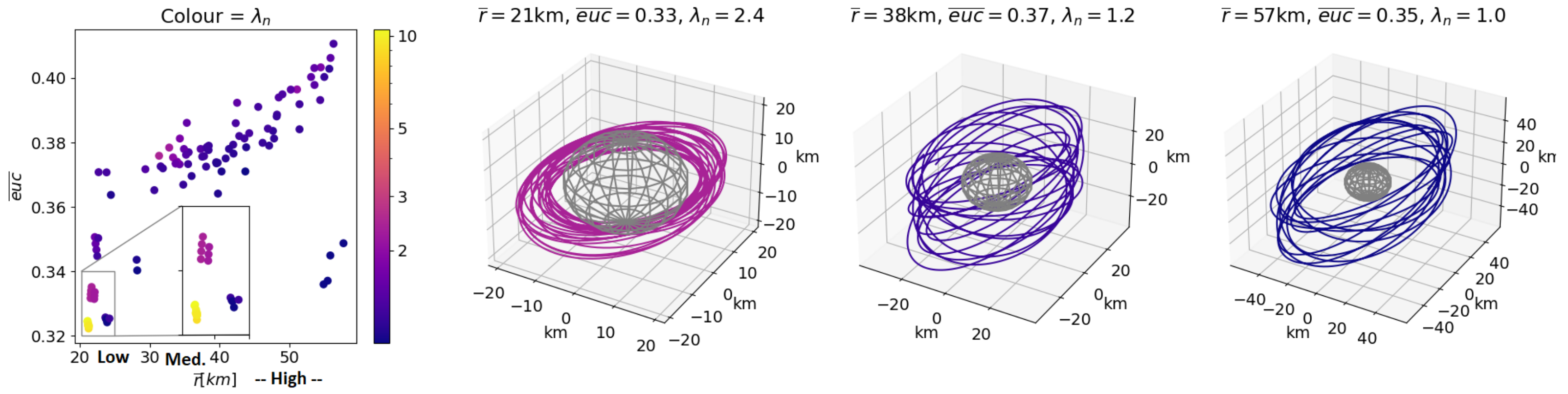
A grid search with a differential corrector step (details in [44]) set out to find a set of initial conditions leading to orbits which stay bound to Phobos for one week. This timespan can guarantee an acceptable geodetic solution accuracy, without incurring excessive costs in terms of orbit maintenance and computational runtime. The search yielded a total of 7000 suitable initial conditions; to make this number compatible with parameter estimation without sacrificing the diversity in orbital geometries, these solutions were classified in accordance with three objectives:
- Proximity, expressed by the mean distance between Phobos’ CoM and the spacecraft (). Close orbits are expected to perform well in the estimation as the gravitational influence on the spacecraft is more pronounced.
- Coverage, computed as the mean euclidean norm of all ground track points mapped in latitude and longitude space (). This is desired to better observe the moon’s surface and decorrelate the influence of individual harmonics.
- Stability, expressed by the largest modulus of the eigenvalues of the state transition matrix after one period. This matrix expresses the linear mapping of the spacecraft state after one period, and its eigenvalues indicate the stability to initial perturbations. This quantity has been normalised by the number of revolutions to ensure a fair comparison across the orbits, i.e.,
A non-dominated objective sorting algorithm yielded a subset of 102 optimal solutions, also known as a Pareto Front (PF). This is depicted in Figure 1 with three representative orbits. The “low” orbits generally have an unfavourable coverage and a precarious stability, “high” orbits display the opposite, and “medium” orbits somewhere in between. Finally, a sensitivity analysis was performed to investigate the robustness of the PF solutions with regard to injection and dynamical model errors. The associated maintenance budgets were validated against those obtained from the above literature.
4. Cold Atom Interferometry
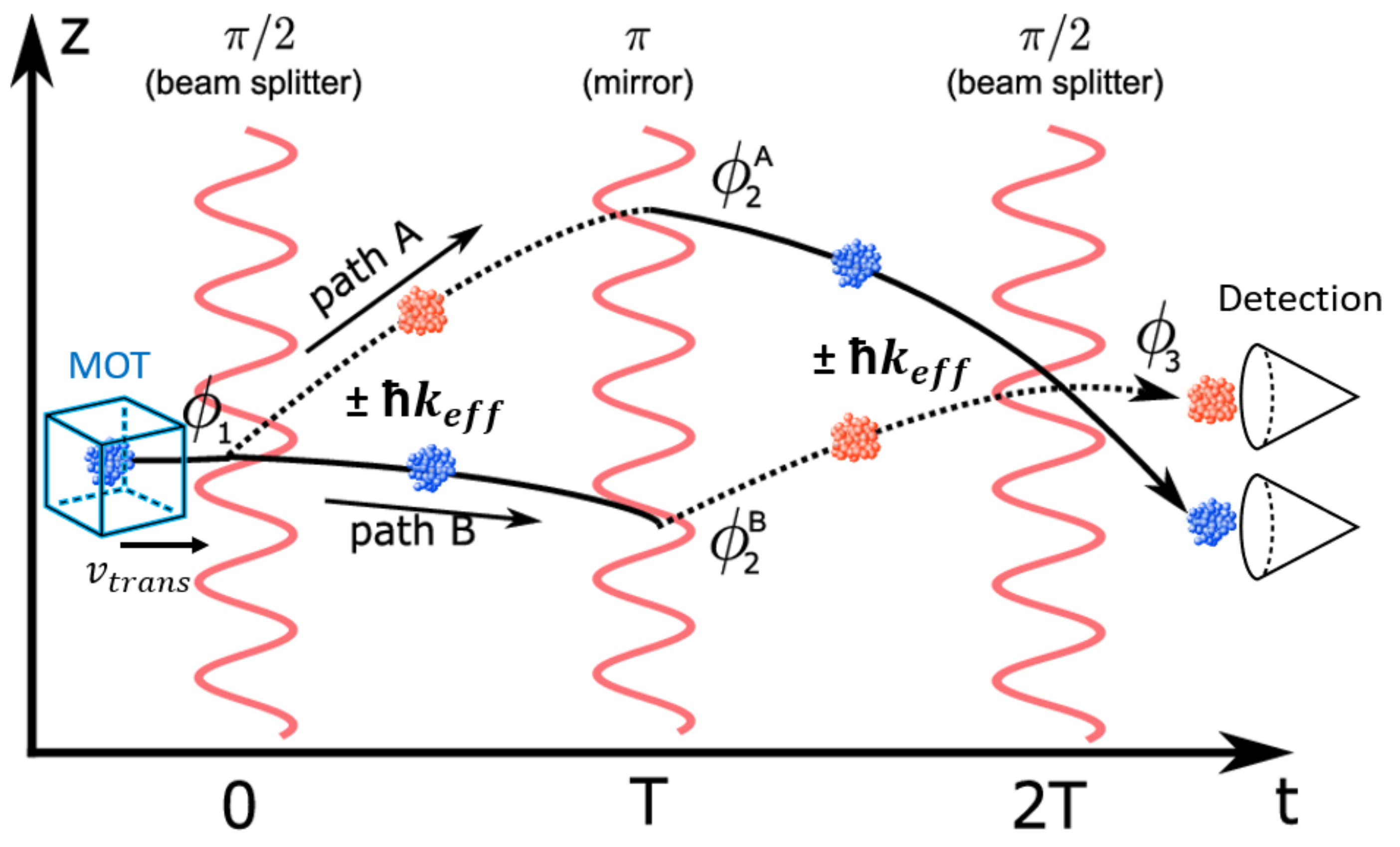
The considered Mach–Zehnder type interferometer with Raman diffraction is shown in Figure 2. A Magneto-Optical Trap (MOT) captures the atomic cloud and cools it to extreme temperatures that are needed to manifest the wave duality of atoms. Inside the interference chamber, the momentum conservation between the atoms and the light field entails that any absorption (emission) of a photon with Raman momentum vector must result in a momentum recoil of () [10]. The first pulse acts as a beamsplitter, causing an equal superposition of quantum states propagating freely along two paths. A second pulse applied at time T fully inverts the states of the two populations, delivering photon recoils to both clouds to rejoin them at time 2T. The last Raman pulse closes the interferometer sequence. Due to the different gravitational acceleration acting on the paths, a phase difference is accumulated, which is recovered at the output ports by monitoring the normalised population in the two hyperfine states.
An additional pulse may be added, separating the initial cloud by a baseline d, such that two measurements are obtained in gradiometric fashion. This suppresses common vibration noise sources such as light shifts and magnetic field gradients [5]. Assuming a detection noise at the quantum projection limit, the gradiometric sensitivity is:
where the total measurement time is required for cooling. The dependency highlights the readout accuracy gained by operating CAI in microgravity. However, the rotation experienced by the CAI setup, coupled with the non-zero transverse velocity, gives rise to an additional phase shift due to the Sagnac effect [10]. This and the thermal expansion of the atomic cloud result in trajectories that do not close perfectly at the third beam splitting pulse, which negatively affects the readout quality. Two strategies can mitigate this effect (detailed in Appendix B), yielding the concepts in Table 3.
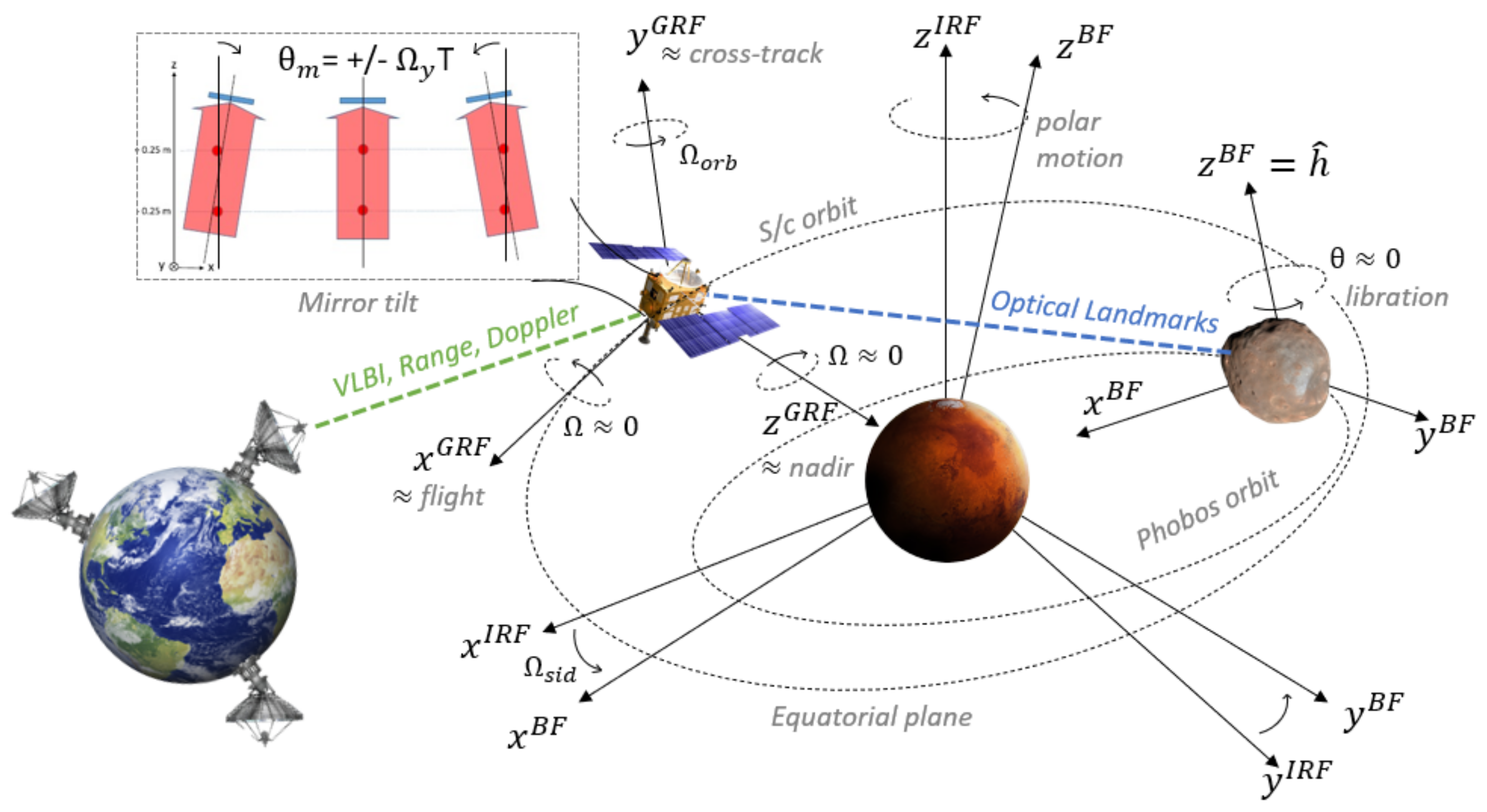
CAI 1 reaches ultracold atomic temperatures via Delta Kick collimation techniques [52] curtailing the need for rotation compensation. This yields a relatively simple setup with a high measurement rate, albeit with limited sensitivity. CAI 2 is based on rotation compensation that imposes an attitude and tilt-mirror control of 1 rad/s and 5 rad along the y axis, respectively, as depicted in Figure 3. This requirement is within the capabilities of fibre optic gyrometers of the ASTRIX 200 class and commercially-available star trackers. Weight and power estimates are adopted from [53] featuring comparable CAI dimensions and sensitivity (reduced values compared to Earth concepts, due to the absence of magnetic shielding and a less demanding cooling mechanism for CAI 2). These estimates are deemed impractical for interplanetary missions, nonetheless, ongoing technological developments are expected to significantly reduce these values. In fact, Ref. [54] aim to produce laser-cooled atoms on a CubeSat platform weighing just over 4 kg and consuming 40 W, albeit for higher atomic temperatures.
To contextualise the performance of the proposed CAI concepts, Table 3 reports the characteristics of GOCE’s electrostatic gradiometer, which enjoys an excellent sensitivity but only in a limited frequency bandwidth. Moreover, the latter suffers from bias instabilities, mainly due to temperature dependencies which affect the long-term stability of the measurements. Broadening the comparison, the current state-of-the-art accelerometer flies on ESA’s Laser Interferometer Space Antenna (LISA) Pathfinder [55] mission. Assuming a distance of 0.5 m between proof masses and a frequency bandwidth (imparted by Phobos’ and above) between and Hz, one may extrapolate a LISA-equivalent gradiometer sensitivity of less than mE. This performance is so outstanding, in fact, that Phobos’ gravity signal would become indistinguishable from the noise due to Mars’ gravity field uncertainty (see Appendix C). Several questions must be addressed before undertaking numerical simulations with a LISA gradiometer: (1) What are the logistical challenges associated with operation? (2) How accurately must the angular velocity be known to distinguish the gravity signal from the centrifugal acceleration? (3) What are the potential satellite-instrument coupling errors when orbiting around a body instead of a Lagrange point? These are left as interesting recommendations for future work.
5. Methodology
This section introduces the setup of the numerical simulations for gravity field recovery. The underlying mechanism for the parameter covariance calculation is described, along with the tracking settings and a summary of the sought parameters. Finally, the specific implementation of the RS and CG experiments is discussed.
5.1. Mission Setup
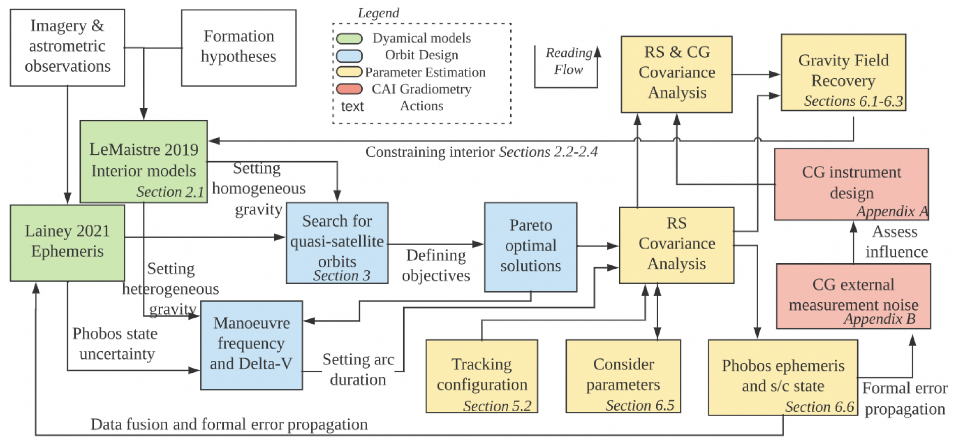
An overview of the setup driving the investigation is provided in Figure 4: two methodological distinctions are highlighted. Phobos’ ephemeris [42] rests on the assumption of a homogeneous interior, which is deemed the most statistically representative and is unaffected by high correlations on its degree-2 harmonics (see Table 2). Thence it is implemented for orbit design and parameter estimation. The heterogeneous interiors are then adopted to assess the maintainability of the candidate orbits, which will constrain the length of the data arcs in the RS experiment (Section 5.5). Another distinction is that RS includes the determination of the spacecraft and Phobos state, which are mapped as external noise on the CG measurements to strengthen the fidelity of the experiment. On the other hand, CG only contributes toward the gravity field solution. By relating to the science goals outlined in Section 2, the extent to which both experiments can constrain Phobos’ origin will finally be addressed.
5.2. Covariance Analysis
The sought gravity field solution influences Phobos’ dynamics, meaning that a full estimation would entail the re-integration of the variational equations at each iteration, which is not ideal considering the vast number of orbits. Moreover, this would result in a random realisation of the probability distribution defined by the covariance, unless dynamical model errors or non-Gaussian noise are introduced. Instead, a covariance analysis is adopted as a means of comparing the formal errors obtained via both experiments. After all, RS is an ineluctable part of all missions, hence the relative contribution of CG plays a stronger role than the absolute accuracy of the solution. The formal errors are obtained from the diagonal of the covariance matrix [34]:
with the design matrix (or Jacobian) and the weight matrix for the measurements. Here, we assume uncorrelated measurement noise, so that is diagonal. The orbital geometry cannot guarantee a full coverage, which may lead to ill-posedness in the estimation, especially for low-power harmonics.
This is avoided by introducing a priori knowledge via as done in Section 5.4. A potent strategy to account for the effect of unmodelled, systematic errors is to set up a consider covariance analysis. Parameters are appended to the covariance calculation process without actually being estimated. Instead, their uncertainty is mapped onto the covariance [34] as follows:
here is the Jacobian for the so-called consider parameters (see Table 4 whose covariance is the diagonal of . Note that their influence does not reduce with more observations, hence they act as a lower limit for the noise. This approach is adopted for RS and CG experiments in Section 6.5 and Appendix C, respectively.
5.3. Tracking Data
Tracking is performed via a combination of radiometric measurements originating from ground stations in Norcia (Australia), Robledo (Spain) and Goldstone (USA), as well as angular landmark positions obtained via optical imagery acquired by the spacecraft itself.
Doppler observables are modelled with a random noise of 30 m/s at 60 s integration time, which is typical for a two-way X-band system at favourable Sun–Earth–Mars angles [40,56]. The integration time can be tuned to balance the measurement volume and noise, which reduces with ≈. Range observables, being an absolute measure of distance, are sensitive to random errors as well as biases [57]. Based on X-band performances [58,59] a 2 m random noise and bias is set, and a cadence of 300 s. The spacecraft’s angular position is determined via Very Long Baseline Interferometry (VLBI), whose bias and noise levels are set to nrad with a cadence of 300 s [60].
Optical landmark tracking is very effective for targets that present distinctive surface features, like craters or boulders. Measurements display a strong sensitivity in the direction perpendicular to the line-of-sight, strongly supporting the retrieval of shape, rotation and ephemeris models as done for Eros [61] Vesta [56] and Bennu [62]. These data are influenced by uncertainties in the spacecraft position and camera pointing, which are hard to decouple. Moreover, merging optical and radiometric data is difficult as the former are dependent on the a priori knowledge of the shape and ephemeris of the body [63]. To this end, the effect of different pointing errors and biases (0.1–0.5 for MEX [64]) is investigated in Section 6.4. A total of 25 landmarks are scattered in latitude ranges , in accordance with Phobos’ shape models [30]. Similar to Vesta, images are captured every 5–10 min which is an optimistic assumption to compensate for the short mission duration. Since the spacecraft will tend to align with Mars, frequent pointing calibrations will be needed for imagery, yet these are deemed feasible as the relative velocity with respect to Phobos is of a few m/s.
5.4. Estimated Parameters
The full set of estimated and consider parameters is reported in Table 4.
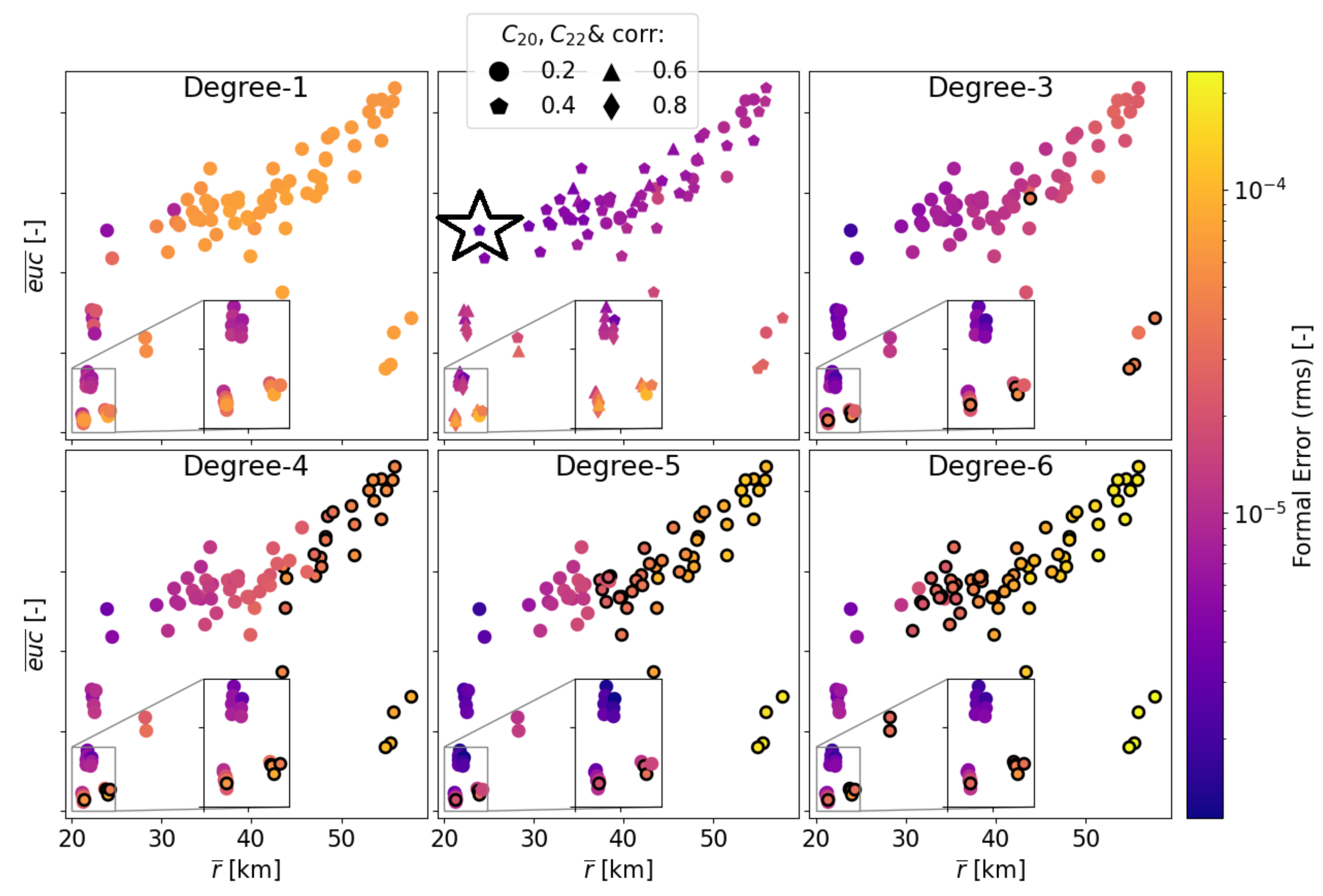
Setting a priori constraints for the gravity field is complicated by the lack of empirical evidence for the gravity spectra of small bodies. In fact, only Eros [61], Vesta [56], Ceres [28], and Bennu [59] have both gravity and shape accurately described. The Kaula rule is typically used for this intent, however, it was derived under the assumption of random point sources in the Earth’s “spherical” mantle, so it becomes invalid for small bodies [66]. They suggest a valid alternative relies on shape models and interior density assumptions, as long as the former are of higher order, a conservatively high value for the radius is chosen, and that the coefficients go to zero (in the mean) to satisfy Parseval’s theorem. Therefore, the maximum standard deviation of the spherical harmonics from the heterogeneous ensembles (i.e., from [14]) were set as a priori values for gravity. Most such values are traced back to the porous compressed interiors, exhibiting the largest spread. With a priori constraints, CG was able to infer the 10 × 10 spectrum (Section 6.3), whereas for RS-only this had to be truncated to degree-6, with the covariance forcing higher terms to zero as to prevent an ill-posed estimation (Section 6.1). As reported by the circled markers in Figure 5, degree-6 is where the formal errors cross the a priori values for a majority of orbits, whilst still ensuring a tolerable condition number for the gravity field columns in the inversion.
Figure 5.
Gravity field recovery via RS at 24 h/day tracking capacity. Vertical and horizontal axes indicate coverage and proximity of the orbital solutions. The formal error root-mean-square is grouped per degree. Shapes reflect the correlation between and . Circled markers indicate that the formal errors cross the a priori standard deviations for all coefficients at that degree. The star denotes the best orbit in terms of accuracy across degrees 1 to 3, further expended in Figure 6.

Two sets of consider parameters have been included. The first comprises the ground station positions, which are affected by uncertainties at the mm level even after correction for tidal and antenna deformation effects. The second are empirical accelerations, which absorb any unmodelled forces that cannot suitably be described due to limited knowledge of the spacecraft’s time-varying orientation, material properties, and surface temperatures [34]. Here, one is concerned with the risk that empirical accelerations will mask the gravity signal from high degrees. These are modelled as 3-axis constant and sinusoidal components with amplitudes as with missions to Eros and Mars (for axes that are unaffected by drag, [40]). Their lowest covariance values match that of OSIRIS-REx at Bennu, which is deemed optimistic, yet feasible in case a detailed panelled thermal radiation model is available. After their consider influence is assessed, their a priori is fixed and they are included in the regular estimation.
5.5. Hybrid-Arc Parameter Estimation
The spacecraft and Phobos states are estimated simultaneously, entailing a hybrid-arc approach whereby the dynamics of the spacecraft and Phobos are integrated into a multi-arc and single-arc fashion, respectively [67]. This offers the distinct advantage of incorporating all dynamical couplings, thus reducing the risk of misattributing a signal in the spacecraft’s dynamics to Phobos’ dynamics which is significant as both are dominated by Mars’ gravity. For the spacecraft, long arcs may lead to convergence issues due to the build-up of unmodelled forces, whereas short arcs may deteriorate the solution quality as not all effects are captured correctly. Arcs may also be sectioned at the manoeuvre times [40] to avoid having to estimate the associated velocity increments. This choice, further validated in Section 6.2, assigns smaller arcs for low orbits, since these are more challenging to maintain (compare in Figure 1).
5.6. Gradiometry
CAI measurements deliver point-wise gravity gradient measurements in the Gradiometer Reference Frame (GRF). These are related to the gravitational potential V Equation (A1) via the observational equation for gradiometry:
although V is tied to the BFF, its second-order partial derivatives (elaborated in [68]) are easily computed in the Local North-Oriented Frame (LNOF). Hence the gradients undergo a sequence of rotations [69]. Since we do not have access to real measurements, the simulator takes a gravitational model and the noise-free time series of the satellite orbit and attitude to set up and where (CAI 1) & (CAI 2). Both configurations are limited to one axis, meaning a single component on the diagonal of in Equation (4) is measured. Ref. [6] have demonstrated that the benefits of 3-axis measurements are concentrated around high-degree harmonics, which is beyond the scope of exploratory missions. It is important to emphasise the axis orientation is not constrained, but merely its uniqueness. Since the nature of the problem does not suggest a prevailing axis for which the gravity signal will be stronger, numerical simulations (Section 6.3) will cover all three cases, and the orientation which leads to the best gravity field solution will be selected.
The superiority of gradiometry over RS in recovering the finer harmonics was hypothesised in [70], who derive analytical expressions to compare the error spectra of both methods. These rest on a number of simplifying assumptions, yet they serve to illustrate the scaling of formal errors as a function of harmonic degree n:
with the Doppler noise, the spacecraft mean motion, and O() a power series of leading order x. This final term confirms the superiority of gradiometry at finer wavelengths. The middle term suggests that gradiometry is harshly affected by an increase in orbital altitude, which was the reason for GOCE’s low altitude (≈259 km) in spite of the adverse atmospheric environment. As a physical analogy, one can imagine that RS is incapable of detecting finer wavelengths, as these do not impart detectable signatures on the trajectory. Conversely, by differencing two closely-spaced accelerations, CG maintains a strong sensitivity to the high frequencies of the gravitational signal.
Four external noise sources affect gradiometry. Attitude control errors limit the ability to overcome attitude disturbances. Attitude knowledge errors hinder the process of geolocating the observables to Phobos’ CoM. For their assessment one must consider rotational dynamics and attitude quaternions for calibration [9] which is beyond the scope here. Instead, a covariance analysis (detailed in Appendix C) was implemented to verify that positioning and dynamical model errors do not compromise the fidelity of the CG experiment.
6. Results and Discussion
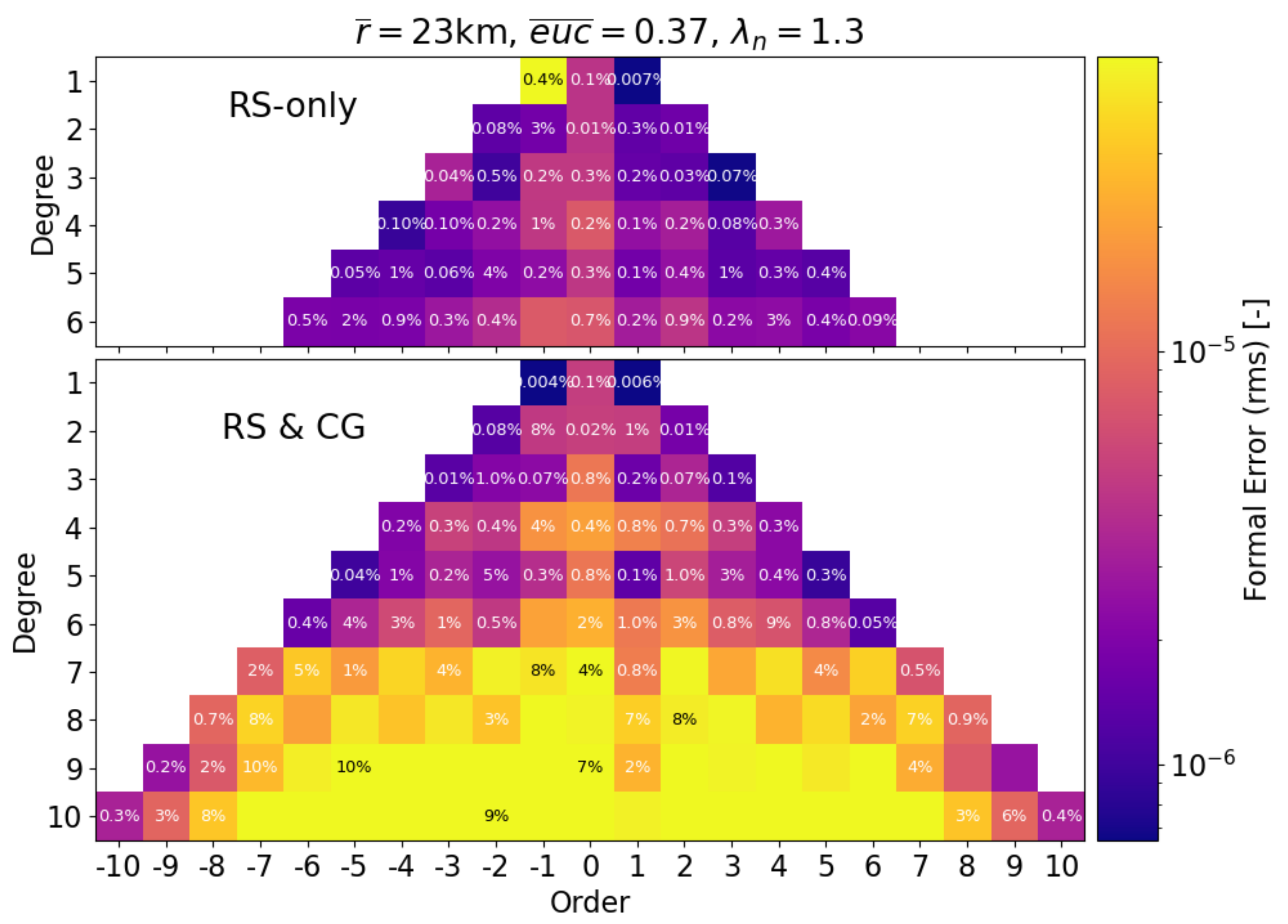
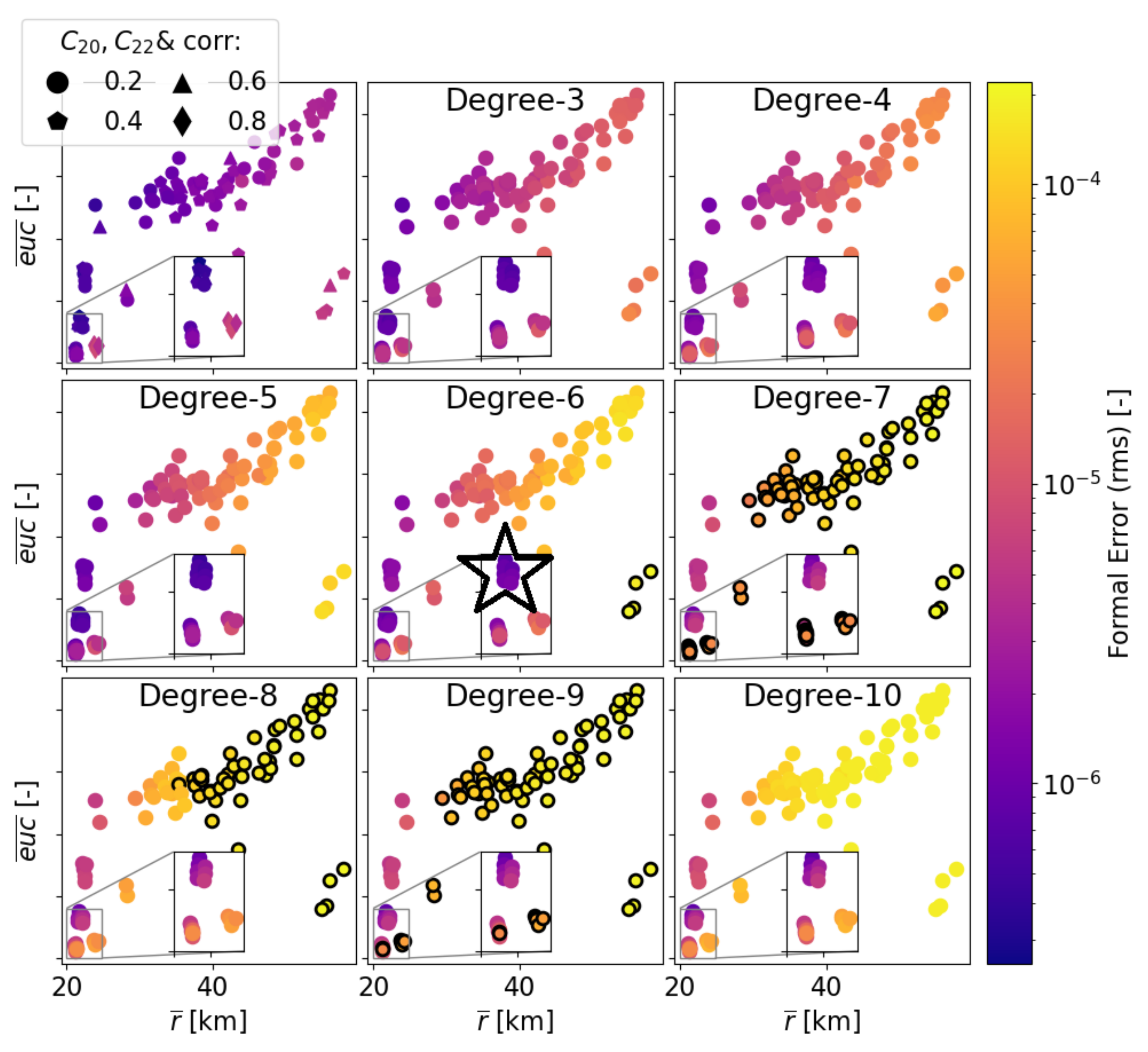
This section presents the outcome of the numerical simulations. The RS-only experiment is outlined in Section 6.1, and summarised in Figure 5 for all orbits in the PF which were generated in Section 3. The RS tracking settings are further tuned in Section 6.2. The combined RS and CG experiment is elaborated in Section 6.3, and plotted in Figure 7. These figures display the (root-mean-square) formal error of the spherical coefficients, grouped per degree. The star markers indicate the “best” case scenario, a compromise between solution accuracy and orbit maintainability, whose full harmonic spectrum is expanded in Figure 6 and Figure 8, respectively. Here, the error is reported as a percentage (x%) relative to the homogeneous values, to address the completion of the science goals formulated in Section 2. In Section 6.4 the contribution of tracking data types is analysed: note that VLBI and range observables have been excluded due to their negligible influence, and that the optical settings were tuned with the altitude to enforce competitiveness across orbits. Moreover, the influence of systematic uncertainties, assessed in Section 6.5 by means of a consider covariance analysis, hints at a true error for RS that is at least 2–3 times higher than the formal one. Finally, Section 6.6 qualitatively discusses the potential improvement of Phobos’ ephemeris and libration from the proposed setups.
6.1. Gravity Field Recovery, Radio Science Only
Figure 5 shows that RS is highly effective for resolving degrees 1 to 6 down to 10 (0.01% with respect to homogeneous), provided that the orbit altitude is kept low. The solution accuracy generally worsens with an increasing degree, yet lower orbits have a geometry that offsets this effect, maintaining a sensitivity to the finer components of the gravitational signal. Orbits with poor coverage underperform even at low altitudes, and tend to rely more on a priori values as reflected by the circled markers (clearly visible for degree-3). The condition number for the overall inversion is between and across the entire PF, mainly driven by the correlations affecting the state of Phobos and the spacecraft. The condition number for the gravity field parameters is between and , which is rather favourable.
Overall, RS seems well suited for recovering Phobos’ gravity field, which is encouraging in the prospect of the MMX mission. Comparing the percentages in the top pyramid of Figure 6 with the spherical coefficient overlap among various interiors ([14],Figures 12 and 13) it is foreseeable that most interiors can be distinguished, except for the rubble pile and icy “evenly distributed” sub-family. The latter only exhibit significant deviations with respect to the homogeneous models at degrees 7 to 9, which are difficult to resolve within one week of observations. Nevertheless, porosity may provide additional clues to discriminate the former, if the interior is monolithic.
Let us now focus more attentively on the individual harmonics. Degree-1 coefficients are resolved to less than 10 (0.01%) translating to an uncertainty in the CoM position of <14 m. At low orbits an accuracy of 10 is made possible by the fact that the optical bias is better resolved with Doppler data (details in Section 6.4) , which expresses the CoM position along (see Figure 3) features high correlations with the spacecraft state estimates. This is because this gravitational signature could be misinterpreted as Phobos approaching the spacecraft since the orbital motion occurs primarily in this (tangential) direction. Our degree-1 estimates are actually conservative since the real Phobos will feature more heterogeneity, meaning their signatures will be larger.
Degree-2 harmonics are inferred accurately to 10 (0.001%) for most orbits. In combination with degree-1, these would certainty (dis)prove a heavily fractured or porous compressed interior, and differentiate most ice-rock mixtures generated by [15]. Note that , , and are omitted from the rms computation, as they are of lower scientific importance (Section 2) and display a smaller signature meaning they would exacerbate the formal errors. Here, coverage plays a primary role in both the accuracy and correlation: the lowest (near-) planar orbits cannot distinguish from , as reflected by the markers’ shapes in Figure 5, nor from GM. Still, it is difficult to draw conclusions on the correlations across the PF due to the limited timeline of the mission and the short arc duration of low orbits (Section 5.5), the individual orbit geometry has a strong influence on the results.
Degrees 3 to 6 are constrained to 10 at low altitudes ensuring a good coverage, which is required to capture Phobos’ gravity variations at non-equatorial latitudes. It must be reckoned that the inclusion of these terms significantly increases the condition number for the inversion, especially for low-inclination orbits (see pink orbit in Figure 1). This is attributed to the fact that degree-2 and 4 coefficients display a similar temporal signature for satellites in a (near-)circular and (near-)equatorial orbit [71]. The same behaviour is visible for degrees 3 and 5, as well as degrees 4 and 6 of the same order. The inclusion of degree-7 and above terms would bias more solutions towards the a priori values, which should not be further restricted due to the high degree-to-degree variability in the models. Theoretically, one could attempt their recovery via the non-circled solutions in the degree-6 Figure 5, whose solution accuracy is slightly optimistic as these higher terms are neglected. Nonetheless, the current estimation is performed assuming a homogeneous interior, whereas the actual Phobos will present more heterogeneity. Hence many real coefficients will display a stronger signature, meaning the absolute solution accuracy will likely be higher, countering the former aspect.
6.2. Tracking Settings Adjustment
A two-step sensitivity analysis of the tracking settings was performed to investigate the robustness of the RS experiment. First, the arc duration was extended to test if the inclusion of additional tracking data would favour the estimation of higher harmonics. This was not the case, and instead proved to exacerbate the influence of systematic errors via the mismodelling of empirical accelerations (Section 6.5). Shortening the arcs did not yield benefits either: evidently, the gravity field signatures are best captured with arcs of 1–2 days. The present model relies on a state-of-the-art tracking system, with ground stations distributed uniformly around the globe operating 24/7. This is logistically challenging and entails high costs of operation. In fact, the MMX design team reserves 8 h/day for tracking, telecommanding and telemetry downlink [72]. Therefore, the complexity of the tracking system was alleviated. One option would be to reduce the number of ground stations from 3 to 2. However, due to planetary occultation by Mars (and visibility conditions on Earth), this may lead to blackout periods. Due to the short mission timeline, this may unfairly target some arcs more than others. Instead, the tracking time within each arc was reduced to 50% capacity, which mimics the strategy of actual missions whereby observation times are planned ahead to guarantee visibility. Although an average of 12 h/day is relatively high for interplanetary missions, it is deemed reasonable during exploratory phases, where a lot of data are gathered on the gravity field. Moreover, this is feasible for Mars since high-gain antenna pointing is not necessary. The tracking time reduction worsens the estimation accuracy by a factor of 2 in most cases, marginally worse than what one might expect from a theoretical point of view (formal errors worsen with in Section 5.2) probably due to the worsened coverage. The accompanying variation in condition number is unordered: for high coverage orbits, it worsens due to the reduction in observations, whereas for others it actually improves as a priori values gain more weight. Since a 12 h/day tracking capacity is both competitive and realistic, this setting is selected in the remainder of the experiment, displayed in Figure 7 and Figure 8.
6.3. Gravity Field Recovery, with CAI Gradiometry
The two configurations in Table 3 were tested individually along three orientations, for each orbit in the PF, resulting in a vast set of experiments. Considering that each estimation involves a degree-10 gravity field, a number of steps had to be taken to condense these into Figure 7. First, the CAI 1 concept was abandoned as it performed consistently worse than CAI 2 in terms of accuracy. Evidently, its higher measurement rate does not outweigh the sharper sensitivity of the latter. One may thus contemplate relaxing the time required for atomic cooling, which will significantly reduce the power demand in Table 3. Since the formal errors scale linearly with the gradiometric sensitivity equation (Equation (2)), the estimates shown hereafter will improve as CAI technology is enhanced, at least for the parameters where the a priori are inactive. Secondly, given that Figure 5 indicates that RS is highly capable of recovering Phobos’ gravity field up to degree-3 without crossing the a priori, only the CAI orientation leading to the highest accuracy for degree-4 and above was selected. It was noted that the performance of the cross-track orientation is poor (as hypothesised in Appendix B, whereas nadir and along-track display a similar efficacy. With this in mind, one may focus on the individual harmonics more attentively.
Degree-1 is improved by a factor of 10 compared to RS, yielding an accuracy better than . These are not shown here, the reason being as follows. Although theoretically a CoM fit to 1.4 m is achievable, realistically, this knowledge will be overshadowed by the uncertainty in Phobos’ ephemeris. Thence, for all intents and purposes, this improvement is insignificant from a science perspective. Nonetheless, it is important to note that the correlation which existed in for RS has now been removed. Degree-2 errors reduce by a factor of 10–15 with CG, meaning an accuracy surpassing . However, the degree-2 objectives can comfortably be achieved with RS alone, so the scientific repercussions of this gain remain to be further investigated. Perhaps their estimate would be accurate enough to detect the temporal modulation signature of . Comparing the markers’ shapes with Figure 5, it is evident that CG is highly effective for decorrelating and .
Comparing the colour pattern in Figure 7 with that in Figure 5, it is evident that CG maintains a higher sensitivity than RS at high degrees, as hypothesised in Section 5.6. The retrieval accuracy ranges from 10 to 10 (0.01%) for the orbits which guarantee a favourable correlation and proximity. Other orbits lead to high errors for degrees 7 to 9 (<100%) as reflected by the circled markers. This is mainly attributed to the indistinguishable low-power coefficients that are present at these degrees. The condition number for the gravity field terms is between and , namely two orders worse than for RS, yet tolerable nonetheless. Once again, the primary correlations affect the cosine harmonics of the same order, with the addition of degrees 7 with 9, and 8 with 10. Finally, whereas RS presents the lowest correlations at close proximity, for CG this occurs at the upper-left vertex of the PF. Evidently, a uniform coverage gains importance if the full spectrum is to be sampled. The overall accuracy gain from CG is immediately visible from the shading of the pyramids in Figure 8. With this configuration, all overlapping factors between the heterogeneous and homogeneous interiors of [14] can be resolved. In combination with shape models, this would reveal Phobos’ internal mass distribution, strongly discriminating between the various formation hypotheses.
6.4. Contribution of Tracking Data Types
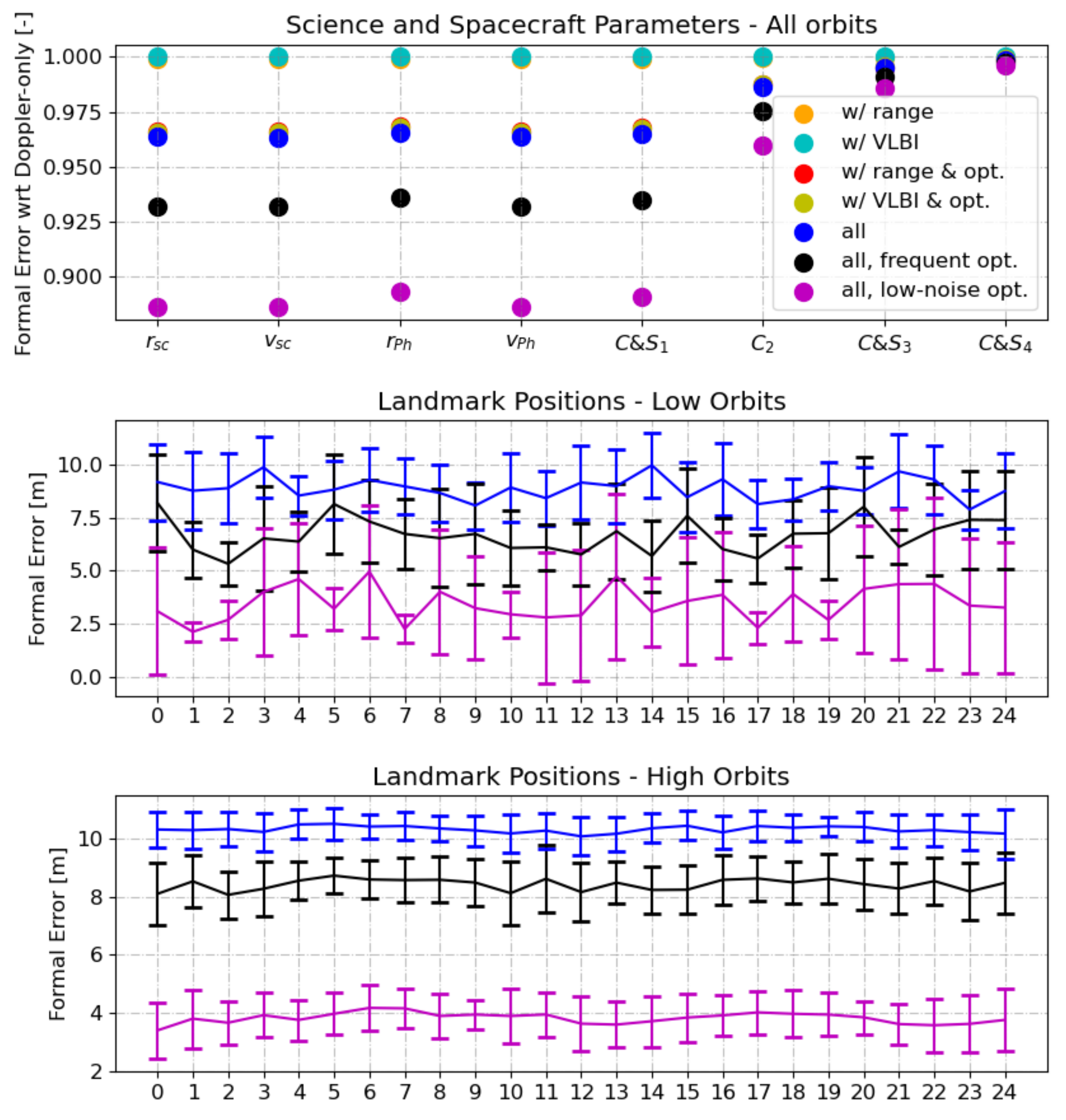
For RS, the onboard transponder design must balance logistical constraints and science return, thence one should investigate the contribution of each data type. This is shown in Figure 9 whereby the formal errors have been normalised with respect to the “nominal” Doppler-only case, due to the different physical scales of the estimated parameters. At first glance one learns that the inclusion of other data types yields a maximum improvement of 10% with respect to the nominal case for all parameters aside from the landmark positions, which can only be obtained via optical measurements (hence these are shown separately).
The superiority of Doppler data for recovering the geodetic parameters is evident. Due to the small characteristic period of the gravity signal, its signatures can only be observed in closely-spaced Doppler measurements [71]. This effect is magnified for higher degrees, as reflected by the narrowing of the markers. Another reason contributing to the superiority of Doppler is related to the observational geometry. The orbit planes of the spacecraft are close to that of Phobos, featuring small inclinations (<30) with respect to Mars’ equator. Consequently, the orbit plane is viewed edge-on from the Earth, meaning velocity changes are effectively captured in the line-of-sight direction. This effect is more pronounced for the low, mostly planar orbits, hence the higher estimation accuracy (see Figure 5). The same could be done for polar orbits with the right precession, however, these are too challenging to maintain. The addition of VLBI and range (“hidden” behind the former) yield no benefit for gravity field determination. Since VLBI measures linear position perpendicular to the line-of-sight with an accuracy in the order of 100 m, its contribution to the gravity field coefficients is negligible [71]. In light of these considerations, range and VLBI data have been omitted.
The inclusion of optical data enhances the state estimate of the spacecraft and Phobos by 4% to 12% depending on the camera settings. Moreover, Phobos’ in-plane orbital components are effectively decorrelated. This is accompanied by an improvement in the degree-1 harmonics since the CoF can better be distinguished from the CoM, which also propagates in the higher-degree spectrum. For the nominal case (blue marker in Figure 9) a 4% improvement in Phobos’ state is accompanied by a 2% improvement in and . This finding agrees with the experiment by the authors of [17], who (inversely) determine that a 2% improvement in Phobos’ CoF position reduces the uncertainty of all degree-2 coefficients by 0.52%. In contrast to Doppler data, the performance of optical tracking depends strongly on the orbit altitude. Low orbits miss many landmarks hence their estimation accuracy is not uniform, as reflected by the error bars in the middle plot. In contrast, the visibility entailed by the high orbits allows capturing the same landmark multiple times. This is highly beneficial for deriving shape and rotational properties as it enables “differenced” landmark observations independent of a priori shape models [62]. At high orbits, the camera performance plays a stronger role because the optical noise (particularly the bias) scales with altitude. This is harder to estimate with Doppler data, which is sensitive to the radial distance from Phobos, as its gravity influence is now weaker. It is therefore not surprising that OSIRIS-REx at Bennu is fitted with three cameras, each tailored to operate in a specific mission phase. The high orbits perform global mapping and shape determination while the closer ones focus on sample-site characterisation [73]. To mimic this behaviour and enforce competitiveness across the orbits for both experiments, the optical settings were tuned with the altitude: low orbits capture more images, whereas high orbits benefit from a lower noise.
6.5. Influence of Consider Parameters
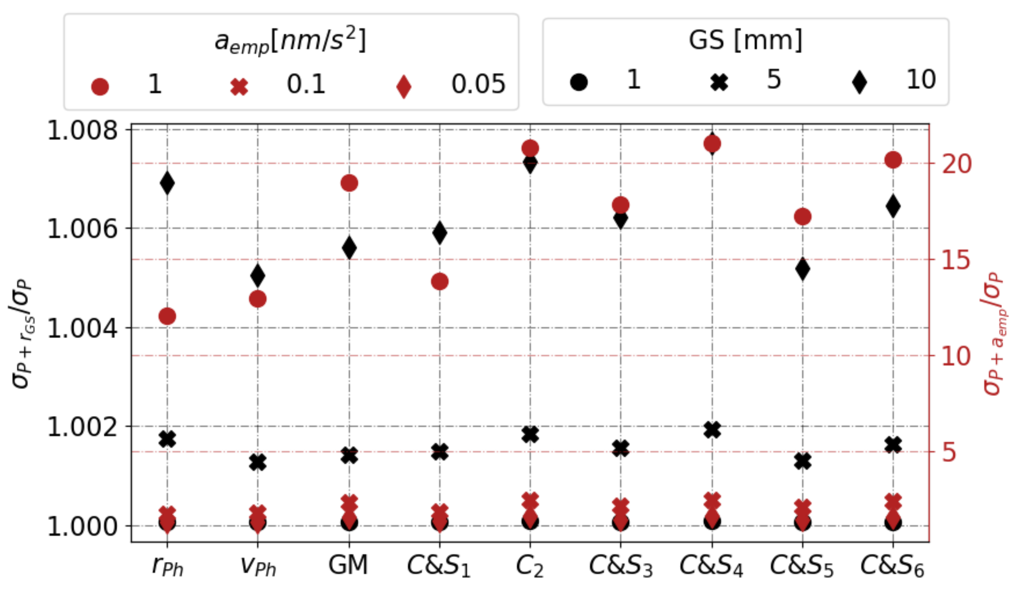
The relative loss in estimation accuracy due to the influence of systematic uncertainties, here taken into account by means of the consider parameters, is reported in Figure 10. Here, the averaged values across the PF are shown (since the trend is similar) although it should be noted that higher orbits are worse affected as their overall formal errors are larger.
Evidently, the ground station position uncertainty is negligible. This is primarily due to the fact that absolute measurements (range and VLBI) have been disregarded. The only concern is Phobos’ state estimate (also affecting the low degree harmonics) that could degrade by ≈1% for an uncertainty of 1 cm. Nonetheless, the latter is rather pessimistic of what can be achieved nowadays ([32] use 5 mm).
The risk associated with the mismodelling of empirical accelerations is severe, with formal errors degrading by a factor of 2–3 in the favourable case whereby 0.05 nm/s. Interestingly, this matches the empirical (a posteriori) true-to-formal error ratios for small-body missions to Eros [61] and Vesta [56] which were 2 and 3 for gravity field parameters, respectively. The worst-case scenario of 1 nm/s aggravates the errors by an order of magnitude, which is similar to the ratio determined for Mars orbiters [40] where atmospheric drag modelling errors are responsible for systematic uncertainties. This stresses the need for high-fidelity modelling of non-conservative forces (mainly the radiation pressure) as this has a confounding influence in small-body environments, particularly for lighter spacecraft. Here, the spacecraft dimensions are undefined, hence empirical accelerations are also included as regular parameters to prevent the formal errors from being overly optimistic. Generally, in the low orbits the along- and cross-track empirical accelerations correlate with the radiation pressure as their influence is confounded with gravity, whereas for high orbits their signature is more distinguishable. This is why for OSIRIS-REx the orientation and thermal diffusive properties were detailed so finely that the estimation of empirical accelerations could be omitted in the lowest orbit, to avoid masking the gravity signal [59]. One may therefore conclude that empirical accelerations must be modelled to below the nm/s level as these constitute a significant threat to the RS experiment, especially for the higher orbits. If this is not possible, one must resort to a gradiometer for direct gravity measurements, or an accelerometer to measure stochastic forces and remove their confounding influence in orbit determination, as done for BepiColombo at Mercury [74].
6.6. Ephemeris and Libration
In this study, we estimated the multi-arc dynamics of the spacecraft, along with the single-arc dynamics of Phobos, using a coupled estimation method [67]. Although our model omits the influence of librations (and their uncertainties) on the dynamics and its covariance, our model does include the linking of Phobos gravity field uncertainty to its state uncertainty. From these results, it is found that Phobos’ radial and tangential position with respect to Mars can be constrained to ~1 m for the planar orbits. These are also best suited for decorrelating Phobos’ velocity from its tangential position.
Modelling the long-term improvement in Phobos’ ephemeris requires data fusion of astrometric data [42] and the radiometric data simulated here, which is beyond the scope of this analysis. Moreover, properly accounting for the influence of Phobos’ rotational dynamics on its ephemeris over both the short-term (during the mission; see Section 3) and the long-term would ideally require a coupled translational-rotational model for the propagation and estimation of Phobos’ dynamics [38,75]. At the very least, it would require the estimation of a spectrum of libration amplitudes.
For the same reasons, we have not included Phobos’ rotational dynamics in our estimation. However, the simulated mission in this work would have a strong ability to constrain Phobos’ rotation as this is manifested in three independent datasets: (1) the kinematic influence of rotation on optical observables; (2) the influence of Phobos orientation on its orbital dynamics through coupling with its gravity field, causing a secular drift in its along-track component [29]; (3) the influence on the spacecraft dynamics through coupling with its gravity field. For case (1) the results in Figure 9 allow us to make a preliminary determination of the quality of the rotation estimate. There, we see estimated landmark position accuracy of ~2–10 m (depending on orbital configuration). Comparing to a maximum position deviation as a result of the libration of ~250 m (from 1.1 libration amplitude, 13 km long axis [13], we get a rough uncertainty estimate on the main libration amplitude of ~0.015–0.075 degrees. Whether this estimate will be degraded by the addition of additional estimated parameters representing the rotation, or if causes (2) or (3) listed above will provide even further improvements in the libration, is to be quantified by future work.
7. Conclusions
This work addresses the potential of Cold-Atom Interferometry for Gradiometry sensors (CG) as a means of strengthening the Radio Science (RS) gravity field experiment, using Phobos as a science case. The heterogeneous interiors in [14] served as guidance for outlining the key geodetic observables needed to constrain Phobos’ origin. The homogeneous interior was used to design Quasi-Satellite Orbits (QSO) ranked by proximity and surface coverage, which are strong drivers for the estimation quality. These metrics clash with the orbital stability (see Figure 1), thus requiring periodic correction manoeuvres that constrain the data arc lengths of the RS experiment. The CG experiment, on the other hand, is simulated for two single-axis instruments that trade-off measurement frequency and gradiometric sensitivity.
Due to the limited coverage of QSO, a priori constraints for the gravity field were required, stemming from the maximum standard deviation of the spherical harmonics in the heterogeneous ensembles. Provided that empirical accelerations can be modelled below the nm/s level, RS is able to infer the 6 × 6 spherical harmonic spectrum to an accuracy of 0.1–1% with respect to the homogeneous interior values, as shown in Figure 6. If this correlates to a density anomaly beneath the Stickney crater, as for the heavily fractured and porous compressed models, RS would suffice to distinguish them, especially if supported by a strong estimate for porosity and libration. Significant overlap is present in the harmonics for the rubble pile and icy moon interiors (or a combination thereof) making their spectra indistinguishable up to degree-6. The most significant deviations occur at degrees 7 to 9, which can only be detected via CG flying close to the moon. As illustrated in Figure 8, this would enable recovering the 10 × 10 spectrum (and higher) to an accuracy below 0.1% for most coefficients. In tandem with the topography and spectrometry observations by MMX, these gravity measurements would provide unequivocal clues on Phobos’ origin. It should be noted, however, that technological advancements must alleviate the power and weight requirements of CG to enhance its competitiveness in an instrument trade-off.
Phobos’ shape is unique, yet its dynamical environment presents similarities to that of other moons in the solar system. The JUpiter ICy moons Explorer (JUICE) [76] will be the first spacecraft to orbit an extraterrestrial moon. The higher ends of the gravity spectrum, within reach of CG, would strengthen topography correlation studies to reveal interesting phenomena such as isostatic compensation mechanisms [77]. To this end, the methodology outlined in this work may serve as a foothold to contemplate the role of CG in bolstering the geodetic investigation of future exploratory missions to small moons, particularly those of the giant planets, which are targets for robotic exploration in the coming decades.
Author Contributions
Conceptualization, M.P., D.D., C.S. and O.C.; Formal analysis, M.P.; Supervision, D.D., C.S. and O.C.; Writing—original draft, M.P.; Writing—review & editing, D.D., C.S. and O.C. All authors have read and agreed to the published version of the manuscript.
Funding
This research received no external funding.
Data Availability Statement
Data is available upon request to the corresponding author.
Acknowledgments
The authors would like to thank Sébastien Le Maistre for his valuable insight on Phobos’ interior, and Olivier Witasse for the guidance offered in the preliminary stages of the project.
Conflicts of Interest
The authors declare no conflict of interest.
Appendix A. Gravity Field Potential
A body’s gravitational potential can be expanded into spherical harmonics [78]:
where indicate the observer’s spherical coordinates in the Body-Fixed Frame (BFF), R the reference radius, the normalised Legendre functions of degree n and order m, and the associated spherical harmonic coefficients. For highly irregular bodies alternative formulations exist. Here spherical harmonics are used to ensure consistency with the literature and because the considered orbits lie well outside the circumscribing sphere of Phobos, guaranteeing series convergence. Coefficients at degree distinguish the Centre of Mass (CoM) from the Centre of Figure (CoF) hence non-zero values are indicative of density heterogeneity. Degree-2 values provide insight into the body’s ellipticity and obliquity, whereas higher degrees indicate local mass concentrations.
Appendix B. CAI Interferometer Phase Shift
The impact of physical perturbations on the phase readouts is investigated to address the need for compensation mechanisms as suggested by [7]. The Gradiometer Reference Frame (GRF), fixed to the satellite as illustrated in Figure 3, is orbiting at a nearly constant frequency with respect to the dominant attractor, in this case Mars (although Phobos’s gravity field will prevail for the low orbits, coincidentally, hence the same rotation is experienced). For the sake of simplicity, this work assumes = and . In reality, this is not the case due to strong third-body perturbations and, to a lesser extent, non-conservative forces. Nonetheless, dominates the conversion of the gradiometric measurements from the GRF to the BFF (see Section 5.6, hence this approach correctly deals with the influence of rotations at the leading orders. We discuss in the following the cases with and without compensation for rotation and gradient dephasing.
Without Compensation. Due to the Sagnac effect, the uncertainty in imprints a rotation-induced dephasing on the interferometer flight and nadir axes. The associated loss of contrast is negligible if the separation is much smaller than the coherence length of the atomic wavepackets [7] a requirement expressed in terms of the atomic temperature in Table A1. A secondary effect concerns the dephasing induced by the gravity gradient, for which a similar temperature limit and contrast loss can be derived [79]. To ensure a reliable detection, the combined effect of dephasings must be kept below the quantum projection limit.
With Compensation. An effective means of ensuring a fixed orientation in the frame of the atoms consists in actively tilting the first and the last retro-reflecting mirrors by an angle (see Figure 3). This method calls for external star trackers and gyrometers for measuring angular velocity. Any error in the latter will translate to a misalignment , with the associated dephasing reported in Table A1. The downside of retro-reflecting mirrors are the stringent dynamic requirements for operation, limiting CAI measurements to a single axis. Gravity gradient compensation mechanisms, demonstrated in [80], rely on an adequate tuning of the Raman wavevector at the second pulse. This offsets their influence across the gradiometric phase, nevertheless, small fluctuations persist [7].

Table A1.
Leading phase errors for differential CAI measurements.
| No Compensation | Compensated | |
|---|---|---|
| Any | ||
| Sagnac noise [rad] negligible for | ||
| Gradient noise [rad] negligible for |
Concerning the operational modes, inertial pointing () has been investigated in [6] for CG on Earth. To maintain the readout noise below 1mrad, spurious rotation rates must be kept below < 1.5 rad/s [5] which is extremely challenging from an engineering standpoint, especially considering the strong third body perturbations by Phobos. This concept is abandoned in favour of nadir pointing, for which . Compensation mechanisms are applicable to both nadir and flight directions, which are influenced by . The cross-track axis remains unaffected, meaning a simplified setup composed of fixed and parallel mirrors can be used [7]. Nonetheless, the nature of the problem suggests that this axis will underperform as it will mostly point away from Phobos, as demonstrated by the coplanar orbits in Figure 3.
The measurement time is highlighted as a key trade-off parameter. Extending it is beneficial for the overall sensitivity Equation (1) but it exacerbates the dephasing induced by rotation. Given that each measurement is averaged along the orbital path, longer measurements may not be able to resolve the finer harmonics. Finally, a large comes at the expense of a more voluminous instrument, given that the baseline must accommodate two counter-propagating clouds, , and the length should be , as illustrated in Figure 2.
Appendix C. Influence of External Noise on Gradiometry
Given that the main gravity signal is that of Mars, from which the modulation due to Phobos must be extracted, one must consider the noise on the gravity gradients associated with Mars’ gravity field. To this end, a covariance propagation is set up:
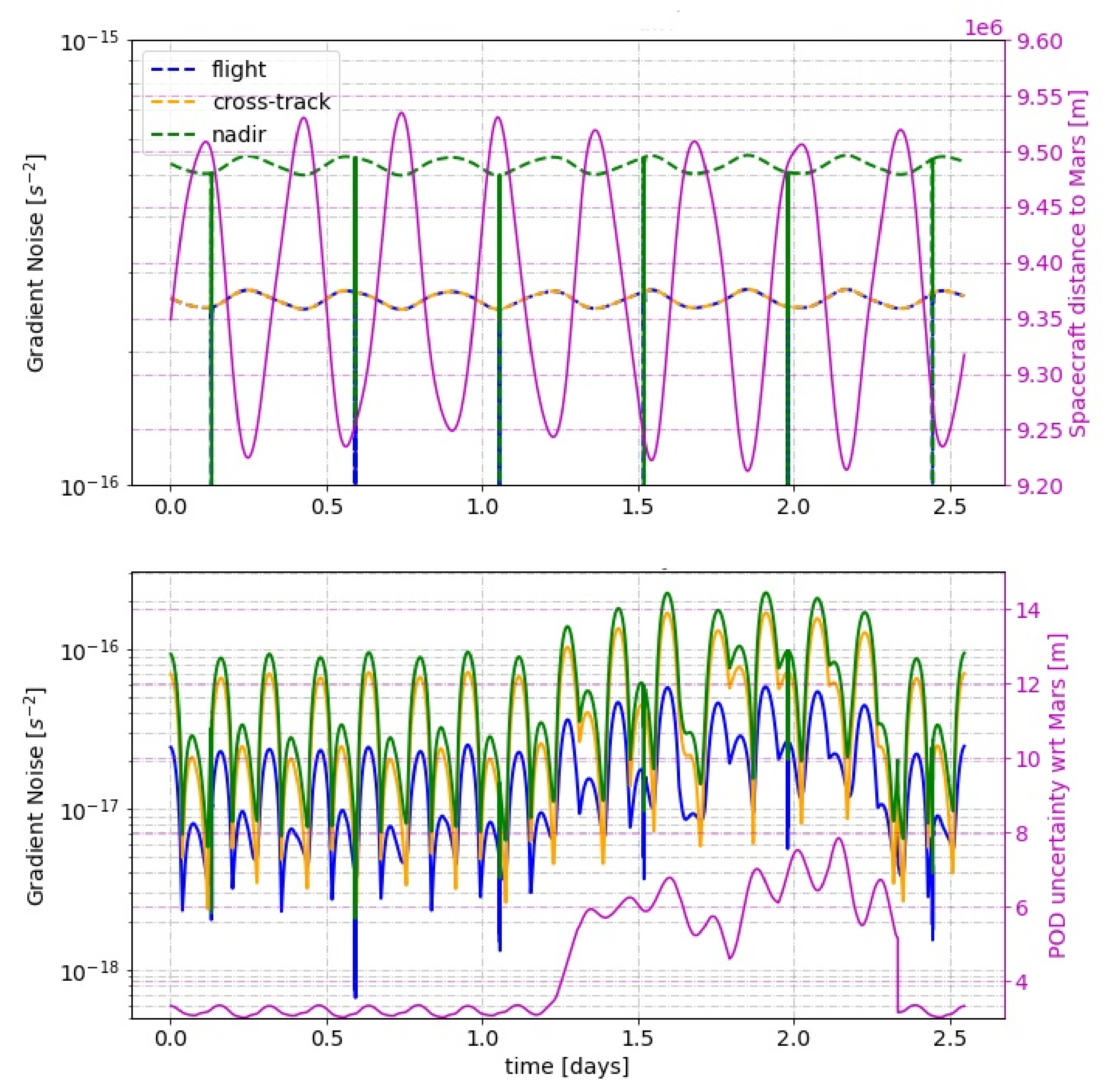
noting that the Jacobian is computed with respect to Mars’ gravity field. Figure A1 illustrates that the dominant noise contribution arises from the orbital eccentricity, acting via the term, as the spacecraft comes closer to Mars. The nadir (z) axis is the worst affected as it is aligned with Mars hence it receives the strongest signal. Still, the noise is far below the gradiometric sensitivity (). A secondary noise source arises from the uncertainty in the spacecraft state with respect to Mars. This is assessed as follows:
whereby the perturbed Jacobian is afflicted by the uncertainty in the spacecraft state with respect to Mars, obtained via formal error propagation. This too is orders below the gradiometric sensitivity, meaning that even if empirical acceleration uncertainties will degrade the spacecraft state estimate (see Figure 10) the gradiometer measurements will remain unaffected. Thence, the true-to-formal error ratio for CG is expected to be close to unity.
Figure A1.
Top: gradient noise from Mars gravity field uncertainty. A single orbit is representative of the entire front since all orbits are similar in the Mars-fixed frame. Bottom: gradient noise from spacecraft state uncertainty, for the worst-case orbit. Note that the arc length is 2.2 days, and tracking ends after 1.1 days (50% capacity) hence the uncertainty is highest after this point.

References
- Pieters, C.; Russell, C.T.; Nathues, A.; Raymond, C.; Jaumann, R.; Castillo-Rogez, J.; De Sanctis, M.C.; Prettyman, T. Evolution of Protoplanets from Detailed Analyses of the Surfaces of Vesta and Ceres by Dawn. In Proceedings of the 42nd COSPAR Scientific Assembly, Pasadena, CA, USA, 14–22 July 2018; Volume 42. [Google Scholar]
- Tricarico, P.; Scheeres, D.; French, A.; McMahon, J.; Brack, D.; Leonard, J.; Antreasian, P.; Chesley, S.; Farnocchia, D.; Takahashi, Y.; et al. Internal rubble properties of asteroid (101955) Bennu. Icarus 2021, 370, 114665. [Google Scholar] [CrossRef]
- Bongs, K.; Holynski, M.; Vovrosh, J.; Bouyes, P.; Condon, G.; Rasel, E.; Schubert, C.; Schleich, W.P.; Roura, A. Taking atom interferometric quantum sensors from the laboratory to real-world applications. Nat. Rev. Phys. 2019, 1. [Google Scholar] [CrossRef] [Green Version]
- Haagmans, R.; Siemes, C.; Massotti, L.; Carraz, O.; Silvestrin, P. ESA’s next-generation gravity mission concepts. Rend. Lincei. Sci. Fis. Nat. 2020, 31, 15–25. [Google Scholar] [CrossRef] [Green Version]
- Carraz, O.; Siemes, C.; Massotti, L.; Haagmans, R.; Silvestrin, P. A Spaceborne Gravity Gradiometer Concept Based on Cold Atom Interferometers for Measuring Earth’s Gravity Field. Microgravity Sci. Technol. 2014, 26, 139–145. [Google Scholar] [CrossRef] [Green Version]
- Douch, K.; Wu, H.; Schubert, C.; Müller, J.; Pereira dos Santos, F. Simulation-based evaluation of a cold atom interferometry gradiometer concept for gravity field recovery. Adv. Space Res. 2018, 61, 1307–1323. [Google Scholar] [CrossRef] [Green Version]
- Trimeche, A.; Battelier, B.; Becker, D.; Bertoldi, A.; Bouyer, P.; Braxmaier, C.; Charron, E.; Corgier, R.; Cornelius, M.; Douch, K.; et al. Concept study and preliminary design of a cold atom interferometer for space gravity gradiometry. Class. Quantum Gravity 2019, 36, 215004. [Google Scholar] [CrossRef] [Green Version]
- Rummel, R.; Yi, W.; Stummer, C. GOCE gravitational gradiometry. J. Geod. 2010, 85, 777–790. [Google Scholar] [CrossRef]
- Siemes, C.; Rexer, M.; Haagmans, R. GOCE star tracker attitude quaternion calibration and combination. Adv. Space Res. 2019, 63, 1133–1146. [Google Scholar] [CrossRef]
- Barrett, B.; Gominet, P.-A.; Cantin, E.; Antoni-Micollier, L.; Bertoldi, A.; Battelier, B.; Bouyer, P.; Lautier, J.; Landragin, A. Mobile and Remote Inertial Sensing with Atom Interferometers. arXiv 2013, arXiv:1311.7033. [Google Scholar]
- Witasse, O.; Duxbury, T.; Chicarro, A.; Altobelli, N.; Andert, T.; Aronica, A.; Barabash, S.; Bertaux, J.-L.; Bibring, J.-P.; Cardesin-Moinelo, A.; et al. Mars Express investigations of Phobos and Deimos. Planet. Space Sci. 2014, 102, 18–34. [Google Scholar] [CrossRef]
- Pätzold, M.; Andert, T.P.; Tyler, G.L.; Asmar, S.W.; Hausler, B.; Tellmann, S. Phobos mass determination from the very close flyby of Mars Express in 2010. Icarus 2014, 229, 92–98. [Google Scholar] [CrossRef]
- Willner, K.; Shi, X.; Oberst, J. Phobos’ shape and topography models. Planet. Space Sci. 2014, 102, 51–59. [Google Scholar] [CrossRef] [Green Version]
- LeMaistre, S.; Rivoldini, A.; Rosenblatt, P. Signature of Phobos’ interior structure in its gravity field and libration. Icarus 2019, 321, 272–290. [Google Scholar] [CrossRef]
- Dmitrovskii, A.A.; Khan, A.; Boehm, C.; Bagheri, A.; van Driel, M. Constraints on the interior structure of Phobos from tidal deformation modeling. Icarus 2022, 372, 114714. [Google Scholar] [CrossRef]
- Guo, X.; Yan, J.; Andert, T.; Yang, X.; Pätzold, M.; Hahn, M.; Ye, M.; Liu, S.; Li, F.; Barriot, J.P. A lighter core for Phobos? Astron. Astrophys. 2021, 651, A110. [Google Scholar] [CrossRef]
- Yang, X.; Yan, J.; Andert, T.P.; Ye, M.; Patzold, M.; Hahn, M.; Jin, W.; Li, F.; Barriot, J.-P. The low-degree gravity field of Phobos from two Mars Express flybys. In Proceedings of the European Planetary Science Congress (EPSC-DPS Joint Meeting), Spokane, WA, USA, 25–30 October 2019; Volume 13, p. EPSC-DPS2019-1521. [Google Scholar]
- Pajola, M.; Lazzarin, M.; Dalle Ore, C.M.; Cruikshank, D.P.; Roush, T.L.; Magrin, S.; Bertini, I.; La Forgia, F.; Barbieri, C. Phobos as a D-type captured asteroid, spectral modeling from 0.25 to 4.0 μm. Astrophys. J. 2013, 777, 127. [Google Scholar] [CrossRef] [Green Version]
- Bagheri, A.; Khan, A.; Efroimsky, M.; Kruglyakov, M.; Giardiani, D. Dynamical evidence for Phobos and Deimos as remnants of a disrupted common progenitor. Nat. Astron. 2021, 5, 539–543. [Google Scholar] [CrossRef]
- Safranov, V.S.; Pechernikova, G.V.; Ruskol, E.L.; Vitjaev, A.V. Protosatellite Swarms. In Satellites; University of Arizona Press: Tucson, AZ, USA, 1986; pp. 89–116. [Google Scholar]
- Canup, R.; Salmon, J. Origin of Phobos and Deimos by the impact of a Vesta-to-Ceres sized body with Mars. Sci. Adv. 2018, 4. [Google Scholar] [CrossRef] [Green Version]
- Rosenblatt, P. The origin of the Martian moons revisited. Astron. Astrophys. Rev. 2011, 19, 44. [Google Scholar] [CrossRef]
- Nallapu, R.T.; Dektor, G.; Kenia, N.; Uglietta, J.; Ichikawa, S.; Herreras-Martinez, M.; Choudhari, A.; Chandra, A.; Schwartz, S.; Asphaug, E.; et al. Trajectory design of perseus: A cubesat mission concept to Phobos. Aerospace 2020, 7, 179. [Google Scholar] [CrossRef]
- Campagnola, S.; Yam, C.H.; Tsuda, Y.; Ogawa, N.; Kawakatsu, Y. Mission analysis for the Martian Moons Explorer (MMX) mission. Acta Astronaut. 2018, 146, 409–417. [Google Scholar] [CrossRef]
- Usui, T.; Bajo, K.I.; Fujiya, W.; Furukawa, Y.; Koike, M.; Miura, Y.; Sugahara, H.; Tachibana, S.; Takano, Y.; Kuramoto, K. The Importance of Phobos Sample Return for Understanding the Mars-Moon System. Space Sci. Rev. 2020, 216. [Google Scholar] [CrossRef]
- Pieters, C. Compositional implications of the color of Phobos. First Mosc. Sol. Syst. Symp. 2010, 123, 43. [Google Scholar]
- Siemes, C. Digital Filtering Algorithms for Decorrelation within Large Least Squares Problems. Ph.D. Thesis, University of Bonn, Bonn, Germany, 2008. [Google Scholar]
- Konopliv, A.; Park, R.; Vaughan, A.T.; Bills, B. The Ceres gravity field, spin pole, rotation period and orbit from the Dawn radiometric tracking and optical data. Icarus 2018, 299, 411–429. [Google Scholar] [CrossRef]
- Jacobson, R.; Lainey, V. Martian satellite orbits and ephemerides. Planet. Space Sci. 2014, 102, 35–44. [Google Scholar] [CrossRef]
- Willner, K.; Oberst, J.; Hussmann, H.; Giese, B.; Hoffmann, H.; Matz, K.D.; Roatsch, T.; Duxbury, T. Phobos control point network, rotation, and shape. Earth Planet. Sci. Lett. 2010, 294, 541–546. [Google Scholar] [CrossRef]
- Shi, X.; Willner, K.; Oberst, J.; Ping, J.; Ye, S. Working models for the gravitational field of Phobos. Sci. China Phys. Mech. Astron. 2012, 55, 358–364. [Google Scholar] [CrossRef]
- Dirkx, D.; Vermeersen, L.; Noomen, R.; Visser, P. Phobos laser ranging: Numerical Geodesy experiments for Martian system science. Planet. Space Sci. 2014, 99, 84–102. [Google Scholar] [CrossRef]
- Dirkx, D. Interplanetary Laser Ranging: A Nalysis for Implementation in Planetary Science Missions. Ph.D. Thesis, Delft University of Technology, Delft, The Netherlands, 2015. [Google Scholar]
- Montenbruck, O.; Gill, E. Satellite Orbits: Models, Methods and Applications; Springer: Berlin/Heidelberg, Germany, 2000. [Google Scholar]
- Rambaux, N.; Castillo-Rogez, J.; Le Maistre, S.; Rosenblatt, P. Rotational motion of Phobos. Astron. Astrophys. 2012, 548, A14. [Google Scholar] [CrossRef] [Green Version]
- Lainey, V.; Duriez, L.; Vienne, A. New accurate ephemerides for the Galilean satellites of Jupiter-I. Numerical integration of elaborated equations of motion. Astron. Astrophys. 2004, 420, 1171–1183. [Google Scholar] [CrossRef] [Green Version]
- Le Maistre, S.; Rosenblatt, P.; Rambaux, N.; Castillo-Rogez, J.C.; Dehant, V.; Marty, J.C. Phobos interior from librations determination using Doppler and star tracker measurements. Planet. Space Sci. 2013, 85, 106–122. [Google Scholar] [CrossRef]
- Dirkx, D.; Mooij, E.; Root, B. Propagation and estimation of the dynamical behaviour of gravitationally interacting rigid bodies. Astrophys. Space Sci. 2019, 364, 37. [Google Scholar] [CrossRef] [Green Version]
- Boué, G.; Correia, A.; Laskar, J. Complete spin and orbital evolution of close-in bodies using a Maxwell viscoelastic rheology. Celest. Mech. Dyn. Astron. 2016, 126, 31–60. [Google Scholar] [CrossRef] [Green Version]
- Genova, A.; Goossens, S.; Lemoine, F.G.; Mazarico, E.; Neumann, G.A.; Smith, D.E.; Zuber, M.T. Seasonal and static gravity field of Mars from MGS, Mars Odyssey and MRO radio science. Icarus 2016, 272, 228–245. [Google Scholar] [CrossRef] [Green Version]
- Konopliv, A.; Park, R.; Folkner, W. An improved JPL Mars Gravity Field and Orientation from Mars Orbiter and Lander Tracking Data. Icarus 2016, 274, 253–260. [Google Scholar] [CrossRef]
- Lainey, V.; Pasewaldt, A.; Robert, V.; Rosenblatt, P.; Jaumann, R.; Oberst, J.; Roatsch, K.; Willner, R.; Ziese, W. Mars moon ephemerides after 14 years of Mars Express data. Astron. Astrophys. 2021, 650, A64. [Google Scholar] [CrossRef]
- Scheeres, D.; Van Wal, S.; Olikara, Z.; Baresi, N. Dynamics in the Phobos environment. Adv. Space Res. 2019, 63, 476–495. [Google Scholar] [CrossRef]
- Chen, H.; Canalias, E.; Hestroffer, D.; Hou, X. Effective Stability of Quasi-Satellite Orbits in the Spatial Problem for Phobos Exploration. J. Guid. Control Dyn. 2020, 43, 2309–2320. [Google Scholar] [CrossRef]
- Baresi, N.; Dei Tos, D.A.; Ikeda, H.; Kawakatsu, Y. Trajectory Design and Maintenance of the Martian Moons eXploration Mission Around Phobos. J. Guid. Control Dyn. 2020, 44, 1–12. [Google Scholar] [CrossRef]
- Pushparaj, N.; Baresi, N.; Ichinomiya, K.; Kawakatsu, Y. Transfers around Phobos via bifurcated retrograde orbits: Applications to Martian Moons eXploration mission. Acta Astronaut. 2021, 181, 70–80. [Google Scholar] [CrossRef]
- Scheeres, D. Orbital Motion in Strongly Perturbed Environments; Springer: Berlin/Heidelberg, Germany, 2012. [Google Scholar]
- Hauth, M.; Freier, C.; Schkolnik, V.; Peters, A.; Wziontek, H.; Schilling, M. Atom interferometry for absolute measurements of local gravity. Proc. Int. Sch. Phys. “Enrico Fermi” 2014, 188, 557–586. [Google Scholar] [CrossRef]
- Floberghagen, R.; Fehringer, M.; Lamarre, D.; Muzi, D.; Frommknecht, B.; Steiger, C.; Pineiro, J.; Costa, A. Erratum to: Mission design, operation and exploitation of the Gravity field and steady-state Ocean Circulation Explorer (GOCE) mission. J. Geod. 2011, 85, 749–758. [Google Scholar] [CrossRef]
- Siemes, C.; Rexer, M.; Schlicht, A.; Haagmans, R. GOCE gradiometer data calibration. J. Geod. 2019, 93. [Google Scholar] [CrossRef]
- Fehringer, M.; André, G.; Lamarre, D.; Maeusli, D. A jewel in ESA’s crown—GOCE and its gravity measurement systems. ESA Bulletin. Bull. ASE. Eur. Space Agency 2008, 2008, 14–23. [Google Scholar]
- Kovachy, T.; Hogan, J.M.; Sugarbaker, A.; Dickerson, S.M.; Donnelly, C.A.; Overstreet, C.; Kasevich, M.A. Matter Wave Lensing to Picokelvin Temperatures. Phys. Rev. Lett. 2015, 114, 143004. [Google Scholar] [CrossRef] [Green Version]
- ESA. Study of a CAI Gravity Gradiometer Sensor and Mission Concepts, Preliminary Design: Reiteration; Doc Number: CAI-TN3; ESA: Paris, France, 2018. [Google Scholar]
- Devani, D.; Maddox, S.; Renshaw, R.; Cox, N.; Sweeny, H.; Cross, T.; Holynski, M.; Nolli, R.; Winch, J.; Bongs, K.; et al. Gravity sensing: Cold atom trap onboard a 6U CubeSat. CEAS Space J. 2020, 12, 539–549. [Google Scholar] [CrossRef]
- Armano, M.; Audley, H.; Baird, J.; Binetruy, P.; Born, M.; Bortoluzzi, D.; Brandt, N.; Castelli, E.; Cavalleri, A.; Cesarini, A.; et al. Sensor Noise in LISA Pathfinder: In-Flight Performance of the Optical Test Mass Readout. Phys. Rev. Lett. 2021, 126, 131103. [Google Scholar] [CrossRef] [PubMed]
- Konopliv, A.S.; Asmar, S.W.; Park, R.; Bills, B. The Vesta gravity field, spin pole and rotation period, landmark positions, and ephemeris from the Dawn tracking and optical data. Icarus 2014, 240, 103–117. [Google Scholar] [CrossRef]
- Thornton, C.L.; Border, J.S. Range and Doppler Tracking Observables. In Radiometric Tracking Techniques for Deep Space Navigation; John Wiley & Sons, Ltd.: Hoboken, NJ, USA, 2003; pp. 9–46. [Google Scholar]
- Iess, L.; Di Benedetto, M.; James, N.; Mercolino, M.; Simone, L.; Tortora, P. Astra: Interdisciplinary study on enhancement of the end-to-end accuracy for spacecraft tracking techniques. Acta Astronaut. 2014, 94, 699–707. [Google Scholar] [CrossRef]
- Scheeres, D.; Mcmahon, J.; French, A.; Brack, D.; Chesley, S.; Farnocchia, D.; Takahashi, Y.; Leonard, J.M.; Geeraert, J.; Page, B.; et al. The dynamic geophysical environment of (101955) Bennu based on OSIRIS-REx measurements. Nat. Astron. 2019, 3, 1. [Google Scholar] [CrossRef] [PubMed]
- Bocanegra-Bahamon, T.M.; Molera Calves, G.; Duev, D.A.; Gurvits, L.I.; Pogrebenko, S.V.; Cimo, G.; Dirkx, D.; Rosenblatt, P. Planetary Radio Interferometry and Doppler Experiment (PRIDE) technique: A test case of the Mars Express Phobos fly-by. A&A 2016, 593, A34. [Google Scholar] [CrossRef] [Green Version]
- Miller, J.K.; Konopliv, A.S.; Antreasian, P.G.; Bordi, J.J.; Chelsey, S.; Helfrich, C.E.; Owen, W.M.; Wang, T.C.; Williams, B.G.; Yeomans, D.K.; et al. Determination of Shape, Gravity, and Rotational State of Asteroid 433 Eros. Icarus 2002, 155, 3–17. [Google Scholar] [CrossRef]
- Goossens, S.; Rowlands, D.D.; Mazarico, E.; Liounis, A.J.; Small, J.L.; Highsmith, D.E.; Swenson, J.C.; Lyzhoft, J.R.; Ashman, B.W.; Getzandanner, K.M.; et al. Mass and Shape Determination of (101955) Bennu Using Differenced Data from Multiple OSIRIS-REx Mission Phases. Planet. Sci. J. 2021, 2, 219. [Google Scholar] [CrossRef]
- Park, R.; Vaughan, A.; Konopliv, A.; Ermakov, A.; Mastrodemos, N.; Castillo-Rogez, J.; Joy, S.P.; Nathues, A.; Polanskey, C.A.; Rayman, M.D.; et al. High-resolution shape model of Ceres from stereophotoclinometry using DAWN Imaging Data. Icarus 2019, 319, 812–827. [Google Scholar] [CrossRef]
- Burmeister, S.; Willner, K.; Schmidt, V.; Oberst, J. Determination of Phobos’ rotational parameters by an inertial frame bundle block adjustment. J. Geod. 2018, 92, 963–973. [Google Scholar] [CrossRef]
- Kosek, W.; Popinski, W.; Wnek, A.; Sosnica, K.; Zbylut-Gorska, M. Analysis of Systematic Errors in Geocenter Coordinates Determined From GNSS, SLR, DORIS, and GRACE. Pure Appl. Geophys. 2020, 177, 867–888. [Google Scholar] [CrossRef] [Green Version]
- Ermakov, A.; Bills, B. Power laws of topography and gravity spectra of the Solar System bodies: Topography and Gravity Power Laws. J. Geophys. Res. Planets 2018, 123, 2038–2064. [Google Scholar] [CrossRef]
- Fayolle, M.; Dirkx, D.; Lainey, V.; Gurvits, L.; Visser, P. Decoupled and coupled moons’ ephemerides estimation strategies—Application to the JUICE mission. Planet. Space Sci. 2022. revision submitted. [Google Scholar] [CrossRef]
- Freeden, W.; Nashed, M.; Sonar, T. Handbook of Geomathematics: Second Edition; Springer: Berlin/Heidelberg, Germany, 2015; pp. 1–3170. [Google Scholar] [CrossRef]
- Siemes, C. GOCE Gradiometer Calibration and LEVEL 1b Data Processing; ESA: Paris, France, 2012. [Google Scholar]
- Bills, B.; Ermakov, A. Simple models of error spectra for planetary gravitational potentials as obtained from a variety of measurement configurations. Planet. Space Sci. 2019, 179, 104744. [Google Scholar] [CrossRef]
- Dirkx, D.; Prochazka, I.; Bauer, S.; Visser, P.; Noomen, R.; Gurvits, L.I.; Vermeersen, B. Laser and radio tracking for planetary science missions: A comparison. J. Geod. 2018, 93, 2405–2420. [Google Scholar] [CrossRef] [Green Version]
- Matsumoto, K.; Hirata, N.; Ikeda, H.; Kouyama, T.; Senshu, H.; Yamamoto, K.; Noda, H.; Miyamoto, H.; Araya, A.; Araki, H.; et al. MMX geodesy investigations: Science requirements and observation strategy. Earth Planets Space 2021, 73, 226. [Google Scholar] [CrossRef]
- Smith, P.; Rizk, B.; Kinney, E.; Fellows, C.; Drouet d’Aubigny, C.; Merrill, C. The OSIRIS-REx Camera Suite (OCAMS). Lunar Planet. Inst. Sci. Conf. Abstr. 2013, 44, 26. [Google Scholar]
- Cappuccio, P.; Di Ruscio, A.; Iess, L.; Mariani, M. BepiColombo Gravity and Rotation Experiment in a Pseudo Drag-Free System. Aerosp. Res. Cent. 2020, 1095, AIAA 2020-1095. [Google Scholar] [CrossRef]
- Borderies, N.; Yoder, C.F. Phobos’ gravity field and its influence on its orbit and physical librations. Astron. Astrophys. 1990, 233, 235–251. [Google Scholar]
- Grasset, O.; Dougherty, M.; Coustenis, A.; Bunce, E.; Erd, C.; Titov, D.; Blanc, M.; Coates, A.; Drossart, P.; Fletcher, L.N.; et al. JUpiter ICy moons Explorer (JUICE: An ESA mission to orbit Ganymede and to characterise the Jupiter system. Planet. Space Sci. 2013, 78, 1–21. [Google Scholar] [CrossRef]
- De Marchi, F.; Di Achille, G.; Mitri, G.; Cappuccio, P.; Di Stefano, I.; Di Benedetto, M.; Iess, L. Observability of Ganymede’s gravity anomalies related to surface features by the 3GM experiment onboard ESA’s JUpiter ICy moons Explorer (JUICE) mission. Icarus 2021, 354, 114003. [Google Scholar] [CrossRef]
- Kaula, W.M. Theory of Satellite Geodesy: Applications of Satellites to Geodesy; Dover Publications: Mineola, NY, USA, 1966. [Google Scholar]
- Roura, A.; Zeller, W.; Schleich, W.P. Overcoming loss of contrast in atom interferometry due to gravity gradients. New J. Phys. 2014, 16, 123012. [Google Scholar] [CrossRef] [Green Version]
- D’Amico, G.; Rosi, G.; Zhan, S.; Cacciapuoti, L.; Fattori, M.; Tino, G. Canceling the Gravity Gradient Phase Shift in Atom Interferometry. Phys. Rev. Lett. 2017, 119, 253201. [Google Scholar] [CrossRef] [Green Version]
Figure 1.
Pareto Front for the non-dominated objective space of proximity, coverage, and stability. Three sample trajectories (low, medium, and high) are plotted in the BFF. The motion is retrograde (clockwise) to curtail the destabilising effect of the term which is “averaged out” in space due to the large relative angular motion between the spacecraft and Phobos [47].

Figure 2.
CAI measurement sequence adapted from [48]. The lines indicate the classical trajectories of the atoms under the influence of gravity, the colours represent two-level internal states.
Figure 2.
CAI measurement sequence adapted from [48]. The lines indicate the classical trajectories of the atoms under the influence of gravity, the colours represent two-level internal states.

Figure 3.
Illustrating the reference frames, rotations, observables and CAI rotation compensation.

Figure 4.
Flowchart summarising the methodology adopted in this work and the relevant sections.

Figure 6.
Formal errors for the gravity spectrum obtained via the best orbit in the RS experiment, marked by a star in Figure 5. This leads to the highest accuracy for degrees 1 to 3, and entails low maintenance costs. Errors are reported as absolute (colour) and homogeneous-normalised (percentage) values. Missing percentages indicate a formal error greater than 100%, some of which correspond to harmonics with very small magnitudes in the homogeneous model (mainly at degrees 7 and 9). Note that the true errors for the top pyramid could increase by a factor of 4–6 due to the influence of systematic uncertainties (see Figure 11) and a reduction in tracking capacity.

Figure 7.
Gravity field recovery for the combined experiment. RS tracking is 12 h/day, CG sensitivity is mE with measurements every 11 s. Shapes reflect the correlation between and . In contrast to Figure 5, here all the formal errors stay below the a-priori standard deviations, hence the circled markers indicate that the formal errors cross the homogeneous values. The star denotes the best (family of) orbits in terms of accuracy across degrees 4 to 10.

Figure 8.
Formal errors for the gravity spectrum obtained via the best orbit in the combined experiment, marked by a star in Figure 7. This is more unstable compared to Figure 6, but the gain in accuracy across the entire spectrum outweighs the associated maintenance costs. Note that the true errors for the top pyramid could increase by a factor of 2–3 due to the influence of systematic uncertainties (Section 6.5).

Figure 9.
(Top): orbit-averaged contribution of tracking data types on formal errors with respect to Doppler-only case for all parameters. (middle and bottom): influence of optical instrument performance (noise and image frequency) on landmark position accuracy. Markers and lines show mean, bars show maximum/minimum values. This figure only concerns the RS experiment.

Figure 10.
Formal error ratio: with(out) consider parameter influence, mean value across the PF.

Table 1.
Working models for Phobos’ gravity field.
| Group | Method | Remarks |
|---|---|---|
| [29] | Dynamical fitting of all astronomic observations, assume [30] libration value | High correlations between and . Rejects heavily fractured and supports porous compressed interior at |
| [12] | RS experiment from MEX flyby in 2010 | Insufficient accuracy due to an unfavourable flyby geometry |
| [17] | Includes 2013 MEX flyby and homogeneous a priori regularisation | Better accuracy and lower correlation. Supports porous compressed interior and [16] lighter core model |
| [13,31] [14] | Based on degree-45 shape model with assumptions on interior density | Modelled, not observed. Complete up to degree-10. Basis for this study |
Table 2.
Adopted dynamical model.
| Mars | |
|---|---|
| Gravitational param. | 42,828.37 km/s |
| Gravity field model | [40] |
| Rotation model | [41] |
| Phobos | |
| Gravitational param. | 7.11 × 10 km/s |
| Gravity field model | [14] |
| Rotation model | Synchronous |
| Ephemeris | [42] |
| Radius | 14 km |
| Semi-major axis | 9378 km |
| Orbital period | 7 h 39 m |
| Eccentricity | 0.0151 |
| Inclination | |
| Start epoch | 1 January 2030 |
| Frame origin | Mars CoM |
| Frame orientation | J2000 Ecliptic |
Table 3.
CAI-based gradiometer configurations, compared with GOCE.
| CAI 1 | CAI 2 | GOCE | |
|---|---|---|---|
| N/A | |||
| 1 pK | 1 nK | N/A | |
| Temperature stability | N/A | N/A | 10 mK over 200 s [49] |
| T | 2.6 s | 5 s | N/A |
| 462 mE | 37.5 mE | 5–100 mHz: 10 mE <5 mHz: noise >100 mHz: noise [50] | |
| Compensation | None | rad | N/A |
| Baseline | 70 cm | 50 cm | 50 cm |
| Laser Diameter | 1.55 mm | 0.25 m | N/A |
| Weight | 163.7 kg | 170.2 kg | 180 kg [51] |
| Power | 480 W | 560 W | 100 W [51] |
Table 4.
Estimated science (top) and mission (bottom) parameters. Note that is first appended as a consider parameter (which are marked with an asterisk), then estimated as a regular parameter.
Table 4.
Estimated science (top) and mission (bottom) parameters. Note that is first appended as a consider parameter (which are marked with an asterisk), then estimated as a regular parameter.
| Parameter Name | Symbol | A Priori Standard Deviation |
|---|---|---|
| Phobos initial state | 100 m, 0.3 mm/s [42] | |
| Phobos landmarks | 12 m from shape models [11] | |
| Phobos gravitational param. | GM | 0.7 km/s from flyby [12] |
| Phobos spherical harmonics | from heter. models [14] | |
| S/c initial states | 50 m, 3 cm/s from MMX [45] | |
| S/c radiation coefficient | 0.1 from Vesta & Eros missions | |
| S/c momentum wheel desat. | 4 cm/s from MEX | |
| Optical biases | 0.1–0.5 | |
| Range biases | 2 m | |
| VLBI biases | 1.5 nrad | |
| Ground station positions * | * 1–5–10 mm [65] | |
| S/c empirical accelerations * | 10 nm/s and * 1–0.01–0.05 nm/s |
Publisher’s Note: MDPI stays neutral with regard to jurisdictional claims in published maps and institutional affiliations. |
© 2022 by the authors. Licensee MDPI, Basel, Switzerland. This article is an open access article distributed under the terms and conditions of the Creative Commons Attribution (CC BY) license (https://creativecommons.org/licenses/by/4.0/).
Share and Cite
MDPI and ACS Style
Plumaris, M.; Dirkx, D.; Siemes, C.; Carraz, O. Cold Atom Interferometry for Enhancing the Radio Science Gravity Experiment: A Phobos Case Study. Remote Sens. 2022, 14, 3030. https://0-doi-org.brum.beds.ac.uk/10.3390/rs14133030
AMA Style
Plumaris M, Dirkx D, Siemes C, Carraz O. Cold Atom Interferometry for Enhancing the Radio Science Gravity Experiment: A Phobos Case Study. Remote Sensing. 2022; 14(13):3030. https://0-doi-org.brum.beds.ac.uk/10.3390/rs14133030
Chicago/Turabian StylePlumaris, Michael, Dominic Dirkx, Christian Siemes, and Olivier Carraz. 2022. "Cold Atom Interferometry for Enhancing the Radio Science Gravity Experiment: A Phobos Case Study" Remote Sensing 14, no. 13: 3030. https://0-doi-org.brum.beds.ac.uk/10.3390/rs14133030
Note that from the first issue of 2016, this journal uses article numbers instead of page numbers. See further details here.