Article

A Year-Long Total Lightning Forecast over Italy with a Dynamic Lightning Scheme and WRF

1
National Research Council of Italy—Institute of Atmospheric Sciences and Climate (CNR-ISAC), via del Fosso del Cavaliere 100, 00133 Rome, Italy
2
CIMA Research Foundation, Via A. Magliotto 2, 17100 Savona, Italy
3
Department of Earth Sciences, Hebrew University of Jerusalem, Givat Ram, Jerusalem 91904, Israel
4
Weather It Is, Ltd., Efrat 91344, Israel
5
Civil Protection Department, via Vitorchiano 4, 00189 Rome, Italy
*
Author to whom correspondence should be addressed.
Remote Sens. 2022, 14(14), 3244; https://0-doi-org.brum.beds.ac.uk/10.3390/rs14143244
Submission received: 9 June 2022 / Revised: 30 June 2022 / Accepted: 2 July 2022 / Published: 6 July 2022

Abstract

:
Lightning is an important threat to life and properties and its forecast is important for several applications. In this paper, we show the performance of the “dynamic lightning scheme” for next-day total strokes forecast. The predictions were compared against strokes recorded by a ground observational network for a forecast period spanning one year. Specifically, a total of 162 case studies were selected between 1 March 2020 and 28 February 2021, characterized by at least 3000 observed strokes over Italy. The events span a broad range of lightning intensity from about 3000 to 600,000 strokes in one day: 69 cases occurred in summer, 46 in fall, 18 in winter, and 29 in spring. The meteorological driver was the Weather Research and Forecasting (WRF) model (version 4.1) and we focused on the next-day forecast. Strokes were simulated by adding three extra variables to WRF, namely, the potential energies for positive and negative cloud to ground flashes and intracloud strokes. Each potential energy is advected by WRF, it is built by the electrification processes occurring into the cloud, and it is dissipated by lightning. Observed strokes were remapped onto the WRF model grid with a 3 km horizontal resolution for comparison with the strokes forecast. Results are discussed for the whole year and for different seasons. Moreover, statistics are presented for the land and the sea. In general, the results of this study show that lightning forecast with the dynamic lightning scheme and WRF model was successful for Italy; nevertheless, a careful inspection of forecast performance is necessary for tuning the scheme. This tuning is dependent on the season. A numerical experiment changing the microphysics scheme used in WRF shows the sensitivity of the results according to the choice of the microphysics scheme.

Graphical Abstract

1. Introduction

Lightning is a hazard to life and properties. In the USA, for example, flashes are as deadly as tornadoes [1,2,3,4,5,6,7,8,9,10,11,12], and in some years, hurricanes, but they are less deadly than floods and flash floods. In Italy, about 20–30 people are killed every year by flashes with even more injured (probably ten times the people killed according to Istituto Superiore di Sanità [13]). Lightning is an important issue for electrical companies, forest fires, and, in general, outdoor activities. The lightning forecast is also important for aviation [14,15] because while airplanes are built to withstand lightning strokes [16], they can suffer structural damage (e.g., [17,18]). Lightning can also affect airport ground operations.
The lightning forecast also gives an indication of the location of severe weather, since high values for total lightning are a good indicator of storm severity occurrence (e.g., [19,20,21,22,23,24,25]). Algorithms to identify total lightning jumps are used to predict severe weather because storms with lightning jumps are longer-lasting and are more likely to develop severe characteristics [11,24,26].
Lightning is a clear manifestation of deep convection as shown by the high lightning activity over the tropical areas in both northern and southern hemispheres [27], as well as by the larger number of flashes recorded in summer (June, July, and August in the northern hemisphere, and December, January, and February in the southern hemisphere), when surface heating forces the development of deep convective cells [28].
A lightning forecast can also be used within a lightning data assimilation [29,30,31]. The forecast of lightning during the assimilation period clearly shows where convection is simulated, helping to precisely address areas where false alarms are predicted. This can be used to reduce spurious convection predicted by models [32].
All of these applications show the potential importance of lightning, suggesting that it needs to be studied, monitored, and predicted.
Different methods have been reported in the literature to forecast lightning strokes from nowcasting to forecasting. Lightning nowcasting from observations is useful to predict flashes from minutes to one hour in the future [33,34,35,36,37,38]. These methods are based on lightning observation networks, where observed flashes are advanced in time to nowcast lightning strokes [35,39,40,41,42,43,44]; alternatively, some approaches use radar reflectivity nowcasting as a proxy for the lightning magnitude [45,46,47,48,49,50]. These nowcasting methods have a useful average lead time of around half an hour [51].
Data assimilation can be used to make highly accurate lightning forecasts from one hour to six hours using numerical weather prediction models (NWP) as, for example, in [31,52]. The same lightning scheme used to make such forecasts can be used to predict lightning for the next day, recognizing that all such forecasts are dependent on the accuracy of convective forecasts at such times.
Methods for forecasting lightning using NWP can be classified into two main groups. The first contains advanced one-dimensional [53,54] or three-dimensional [55,56,57] cloud models equipped with sophisticated electrification schemes. These schemes explicitly simulate the electrification processes and the electric breakdown [58,59]. In [60], Fierro et al., for example, implemented a physics-based, explicit lightning scheme within the Weather Research and Forecasting (WRF) model [61] that treats space charges as state variables and explicitly solves for the three components of the ambient electric field.
The second group includes simpler diagnostic schemes correlating the hydrometeors or other parameters computed by cloud-resolving models with the number of observed flashes [62,63,64,65,66,67]. For example, in ref. [66], Wong et al. revised the Price and Rind parameterizations by applying the same methodology in cloud-resolving models. They showed the need for validation and tuning of the parameterizations when applying the Price and Rind approach to cloud-resolving models. The need for calibration is discussed also in McCaul et al. [68], who compared different settings of the McCaul scheme [63] and recommend methods for its recalibration. These schemes are computationally efficient and show better performance than schemes forecasting lightning based on thermodynamic indices [69], which indirectly describe and quantify atmospheric processes related to lightning [70,71].
Lynn et al. [72] proposed the forecast of lightning through the dynamic lightning scheme (DLS), which is used in this paper. The dynamic lightning model is neither an explicit approach as no electrical field is calculated, nor is it a statistical approach wherein lightning values are calculated directly from the vertical velocity and hydrometeor masses or thermodynamic indices. The DLS uses the dynamic and microphysics fields from WRF to calculate the electrical potential energy for positive and negative cloud-to-ground and intracloud lightning, adding prognostic equations for three variables in the WRF model. The number of cloud-to-ground (positive and negative) and intracloud lightning is computed from these potentials whenever the potential energy is larger than the threshold energy, whose value depends on the type of lightning. According to the tripolar charge model for clouds [73], positive flashes originate from the upper part of the cloud, i.e., the stratiform anvil, negative flashes originate from the lower part of the cloud, and intracloud flashes can occur everywhere in the cloud. Assuming a tripolar charge model, however, is a limitation of the method because the charge structure of deep convection is often more complicated than a tripole [74].
An important parameter of the lightning scheme is the charge transferred in a time unit within the cloud, as shown by the sensitivity tests of Lynn et al. [31]. A complete analysis of this sensitivity is shown in this paper for the specific setting of the WRF model used here and for the Italian area.
Federico et al. [75] showed a lightning forecast over Italy using the RAMS (Regional Atmospheric Modeling System) model equipped with the Dahl et al. [45,76] electrification scheme. However, the aim of their work was limited to showing the feasibility of the method because their paper only evaluated the performance of the lightning forecast for two intense lightning events that occurred during the fall of 2011 and 2012.
This work makes a lightning forecast evaluation over Italy for a whole year using the DLS of Lynn et al. [72]. The analysis is performed for the four seasons within a year and compares the forecast over the land and the sea. A sensitivity test for the fall season shows the impact of changing the microphysical scheme of WRF on the lightning forecast.
This paper is organized as follows: Section 2 gives a short description of the WRF settings and the dynamical lightning scheme and introduces the case studies. Section 3 shows the results, discussing an example of a good forecast, then provides a comparison among the three settings for the DLS, discusses the dependence of forecast performance on the seasons, compares forecasts for over the land and the sea, and finally, discusses the results of a sensitivity numerical experiment aimed studying the impact of the microphysical scheme on the forecast of strokes. Conclusions are given in Section 4 and Appendix A summarizes the statistics used to verify the forecast.

2. Data and Methods

2.1. WRF Model

The numerical model used in this study is the WRF model with Advanced WRF dynamic (WRF-ARW), version 4.1.3 [77]. The simulations use one domain, with 635 × 635 grid points and 50 unevenly spaced vertical levels with a model top at 50 hPa. The model domain (Figure 1) covers the Central Mediterranean and the whole Italian territory. It has a horizontal grid spacing of 3 km. Figure 1 also shows the verification area, extending over Italy and the surrounding sea (6°E–19°E; 36.5°N–47°N).
The physical schemes employed include the Thompson microphysics scheme [78], the Mellor–Yamada–Janjic scheme using a one-dimensional prognostic turbulent kinetic energy scheme with local vertical mixing [79], the five-layer thermal diffusion for land surface processes scheme, the Monin–Obukhov (Janjic Eta) scheme for surface layer physics [80], the Dudhia scheme [81] for the short-wavelength radiative scheme, and the rapid radiative transfer model (RRTM, [82]) for the longwave radiative scheme. No cumulus parameterization was used as these are convection-allowing simulations.
Initial and boundary conditions for the simulations are taken from the integrated forecasting system (IFS) global model of the European Centre for Medium-Range Weather Forecasts (ECMWF). Specifically, we use the analysis-forecast cycle issued at 12 UTC on the day before the actual day to forecast. Hence, for each forecast day, we run the WRF model for 36 h starting at 12 UTC on the day before the actual starting time of the day to forecast. The first 12 h are used for the spin-up of the model and are discarded from the forecast performance evaluation. The initial and dynamic boundary conditions are used at 0.25° horizontal resolution and boundary conditions are updated every 3 h.
To consider the forecast variability with seasons, a total of 162 cases were selected for the year from 1 March 2020 to 28 February 2021. Further details about the simulations of this paper are given in Section 2.3 Case Studies.

2.2. The Dynamic Lightning Scheme and LINET Data

The dynamic lightning scheme (DLS) was proposed by Lynn et al. [72] and is used to simulate both cloud-to-ground (positive and negative) and intracloud strokes. In this paper, we report the main features of the DLS, but the reader is referred to Lynn et al. [72] for a detailed description.
The lightning forecast is computed from the WRF model dynamic and microphysical fields starting from the lightning potential index calculation (LPI, [65,83]). The LPI measures the kinetic energy of updrafts and downdrafts scaled by the potential of charge separations, which is a function of the hydrometeors mixing ratios (cloud, rain, snow, graupel, and ice). Lynn and Yair [83] and Yair et al. [65] specified that the LPI should be computed between the isotherms 0 °C and −20 °C, where the noninductive mechanism involving collisions between ice and graupel in the presence of supercooled water is most effective [84,85]. The LPI has the largest value when graupel exists in an equal ratio relative to water, ice, and snow.
The electric potential is computed by multiplying the LPI by the total mass of ice and dividing by the charge of 1 C (unit of V, J C−1 kg−1). The electric potential is computed for positive, negative, and intracloud lightning. Negative flashes originate from the lower part of the cloud, positive flashes originate from the upper part of the cloud, and intracloud flashes originate everywhere in the cloud. These assumptions are consistent with the tripolar charge model of Williams [73], but more complex electric structures can be present inside the clouds [73].
As the evolution of the cloud progresses, the charge and the electric potential builds up. The source term for this potential is referred in Lynn et al. [72] as the power index and depends on an important constant, whose units are coulombs, such that the appropriate amount of energy builds up over several model time steps. We will refer to this constant as the charge transferred in 1 s inside the convective and stratiform cloud. The number of strokes simulated (and, in some measure, their positions, because the electric potential is advected by WRF) is dependent on these parameters and three different magnitudes of charge transfer were used to calibrate the method as follows: L50, in which the charge transferred in 1 s is 0.5 × 10⁻⁴ C; L75, in which the charge transferred in 1 s is 0.75 × 10⁻⁴ C; and L100, in which the charge transferred in 1 s is 1.0 × 10⁻⁴ C. The three settings were used to simulate all 162 cases considered in this work.
When the potential energy value exceeds threshold values (this value is 5 × 10⁹ J for positive strokes and 1 × 10⁹ J for intracloud and negative strokes), it is converted into electrical energy by lightning strokes (cloud-to-ground or intracloud), immediately dissipating the energy and reducing the electric potential magnitude at that grid point. The same thresholds as Lynn et al. [72] are used. The sum of positive, negative, and intracloud lightning is considered for comparison with observed strokes.
In the DLS, the three electric potentials for positive, negative, and intracloud lightning are formulated in four-dimensional derivative equations so that the scheme can account for energy buildup in convective and stratiform clouds as well as its possible advection from convective to stratiform clouds. For this reason, the scheme was referred to as the dynamic lightning scheme.
Strokes data used to verify the model prediction are provided by the LINET (lightning detection network; [86,87]). LINET includes more than 500 stations worldwide. More than 200 sensors are in Europe, where there is the best lightning detection efficiency. This network covers the Italian territory and the western Mediterranean Sea. LINET sensors detect very low frequency (VLF) and low frequency (LF) waves emitted during a flash. LINET can measure both intracloud (IC) and cloud-to-ground (CG) discharges; nevertheless, in this paper we compare the total strokes observed by LINET with the total strokes simulated by the DLS ignoring the IC-CG difference. The data processing technique used to locate the strokes in three dimensions follows a 3D method ([87]), by which the height of IC lightning is also calculated. Position accuracy is about 75 m for CG and IC strokes.
The detection efficiency (DE) of lightning location networks depends on a variety of parameters, such as the sensitivity of antennae, handling of signals in the receiver, sensor baselines, and treatment in the central data processing unit. In LINET, these components have been optimized to improve IC and CG detection efficiency [87,88]. Among other factors, two characteristics are worth reporting here. First, the LINET sensor measures the magnetic flux of the lightning signal directly as a function of time rather than the time derivative with subsequent integration [87]. Second, LINET uses a time of arrival (TOA) method in the VLF/LF frequency range for lightning detection [86]. Only the arrival times of the signals are used for lightning detection, irrespective of their waveform. The difference of the travel time of high (IC lightning) compared to low (CG lightning) electromagnetic emissions is used for the discrimination between CG and IC and to calculate the emission height of the signals [86,87]. The ability of LINET to detect strokes for the target area, including weak signals (<5 kA), is discussed in [88].
For the above reasons, the DE of LINET is expected to be high over the verification area (hopefully >85–90% for total lightning). Nevertheless, a map showing the DE of the LINET network for different seasons and types of strokes over the verification area is not available and we cannot give a definitive answer about the DE of LINET for this study. For this reason, when comparing the strokes forecast and observations, we use the row LINET strokes without corrections for DE estimations. It is also worth noting that while the DE is high, it is less than 100%, so a small to moderate overestimation (10–15% of the observed value) of the forecasted strokes should be considered as a positive result.

2.3. Case Studies

With the above settings of the WRF model, and with the three settings of the DLS (L50, L75, and L100), 162 cases were simulated for 12 months from 1 March 2020 to 28 February 2021. A total of 486 (162 × 3) simulations were performed, where a change in the DLS setting required a new simulation of the WRF model. These cases were selected to simulate all the days with low, moderate, and high electric activity over Italy. Specifically, this criterion was followed: we focused on the area 6°E–19°E and 36.5°N–47°N (Figure 1) and we considered the number of observed strokes. The days with at least 10,000 strokes were considered for summer and September, and for the other months, the days with at least 3000 strokes were selected. These thresholds were chosen to account for most of the strokes recorded over Italy during the year while avoiding simulating days with marginal lightning activity in different seasons.
The distribution of the cases is as follows: 69 in summer, 46 in fall, 18 in winter, and 29 in spring (Table 1). This distribution is a result of the convection over Italy and the central Mediterranean, which is especially active in summer and fall.
The strokes distribution in different seasons for the whole year and for the subset of 162 cases considered in this paper is shown in Figure 2a. It is apparent that more strokes occur, by far, in summer and fall, followed by spring and winter. From Figure 2a, it follows that the 162 cases are well representative of the seasonal behavior. About 11.5 million strokes were recorded for the 162 cases out of a total of about 12 million that occurred over the whole year. Similar considerations apply to the distribution of the strokes within the hours of the day (Figure 2b), even if this aspect will not be further considered in this work. The 162 cases and the whole year show the strokes peak in the early afternoon (12:00–17:00 UTC, corresponding to 13:00–18:00 local time in winter, November and March, and 14:00–19:00 local time for all other months). This behavior is determined by surface warming, which triggers convective phenomena in summer and fall afternoons.
In addition to the 486 simulations introduced above, the 46 fall cases were simulated with the WSM6 [89] microphysics scheme to assess the impact of changing the microphysics scheme of WRF on the strokes forecast.

3. Results

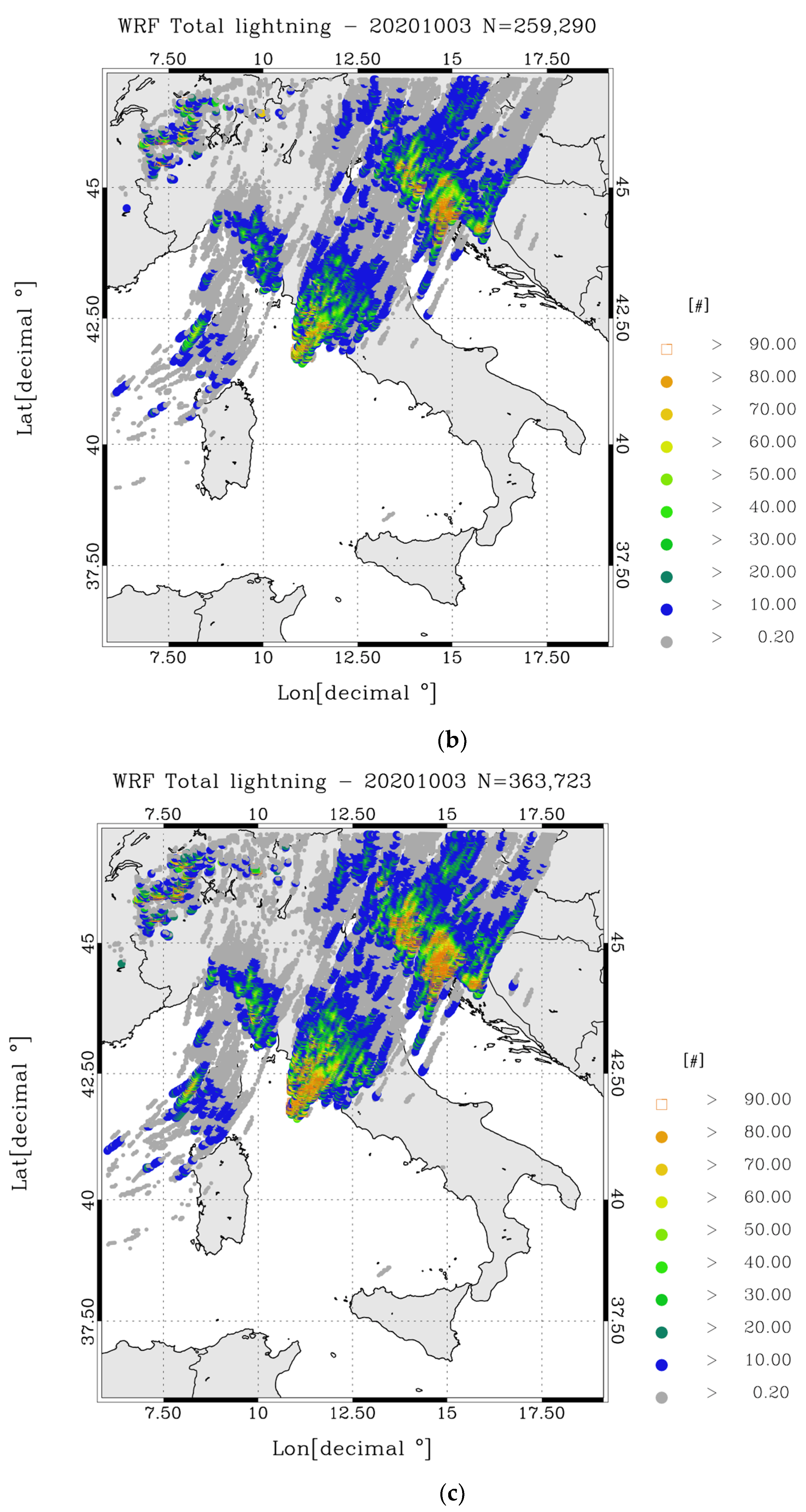
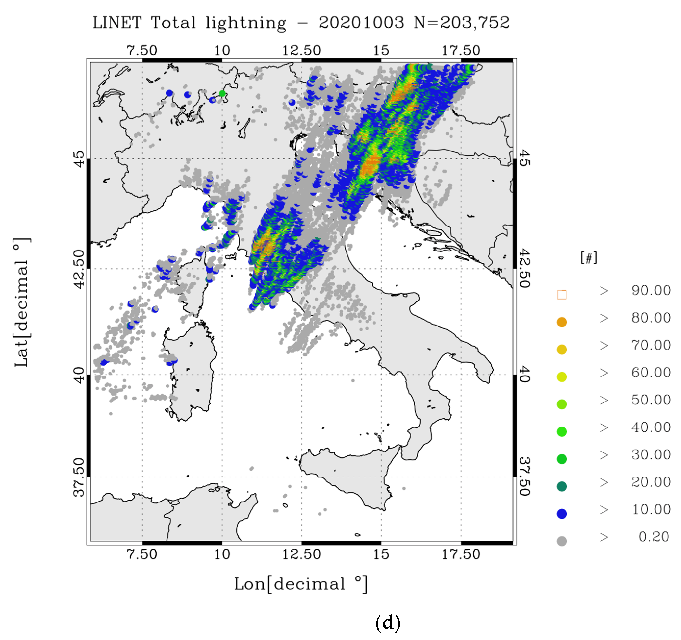
3.1. Example of Predicted Fields

In this section, we show the model output for the stroke density field from 3 October 2020 for the three different charge transfer configurations, L50, L75, and L100 (Figure 3, which shows the daily number of strokes per 9 km2 for the verifications area, i.e., the number of strokes observed/forecasted in a day in each WRF grid cell in the verification area). This was a well predicted event. Observations (Figure 3d) shows intense electrical activity with about 204,000 strokes recorded for the day. The total number of strokes is underestimated by L50, slightly overestimated by L75, and quite overestimated by L100.
The strokes spatial pattern is represented satisfactorily by all settings of the WRF and DLS, with intense electric activity over the Tyrrhenian Sea, Slovenia, and Croatia. For example, considering the scores (for a description of the statistics used in this paper, see Appendix A) for the L75 configuration and a threshold of 1 stroke per WRF grid cell (3 km by 3 km), the probability of detection is around 0.8.
WRF overestimates the electric activity over Liguria, Tuscany, Corse Island, and the Alps. This overestimation is confirmed by the scores: referring to the L75 configuration, frequency bias (FBIAS) is 1.5 for 1 stroke per WRF grid cell for the whole day, and the false alarm rate (FAR) is 0.5 for the same threshold, showing the model tendency to overestimate electrical activity over the area on this day.
As a final remark, we note that despite the different number of strokes predicted by L50, L75, and L100, the spatial patterns of the predicted strokes are similar among the configurations. This result shows that the lightning forecast closely follows the spatial pattern of convection simulated by WRF, even though the occurrence of lightning events is a result of generation and advection of the electric potential in DLS.

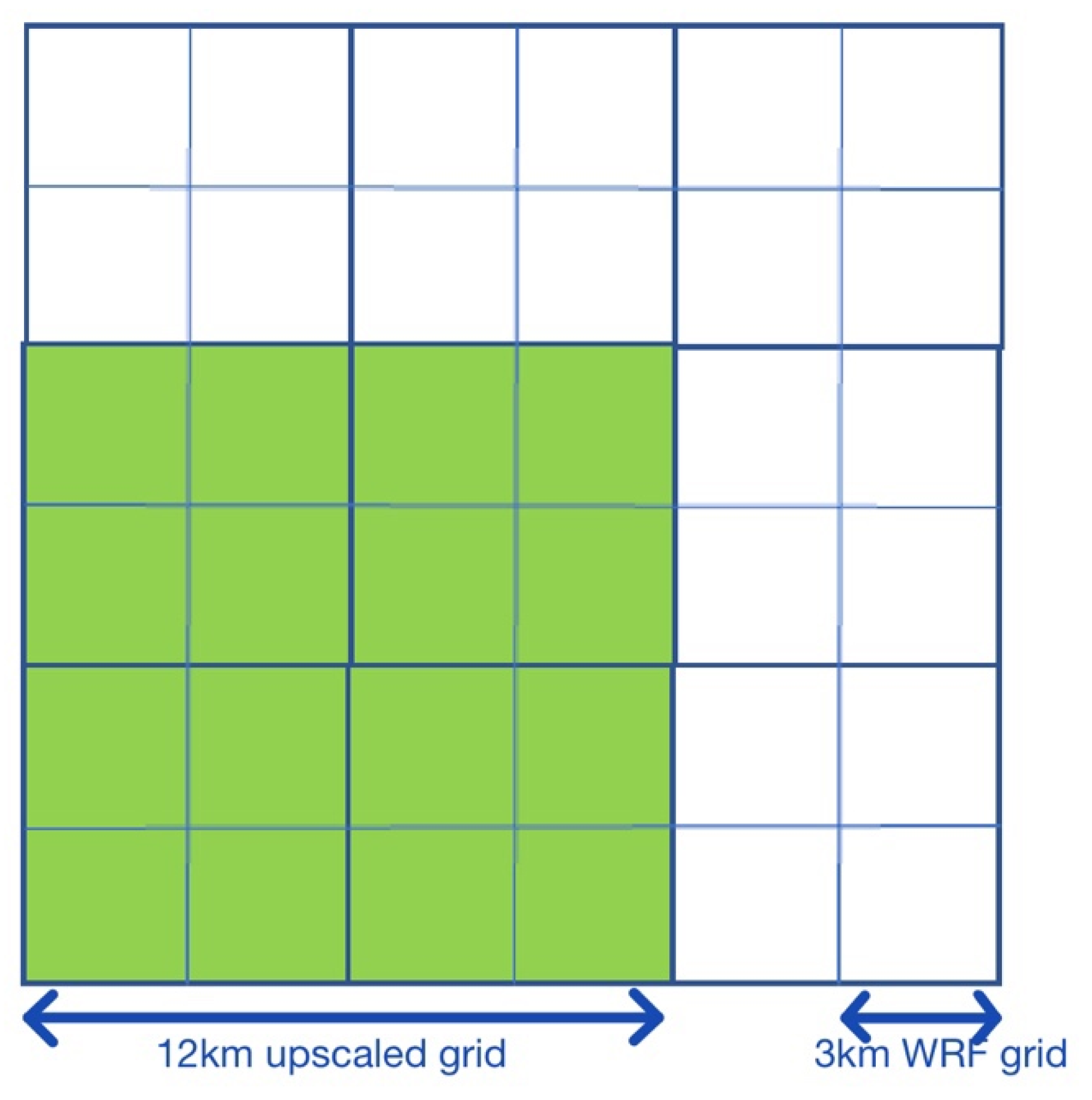
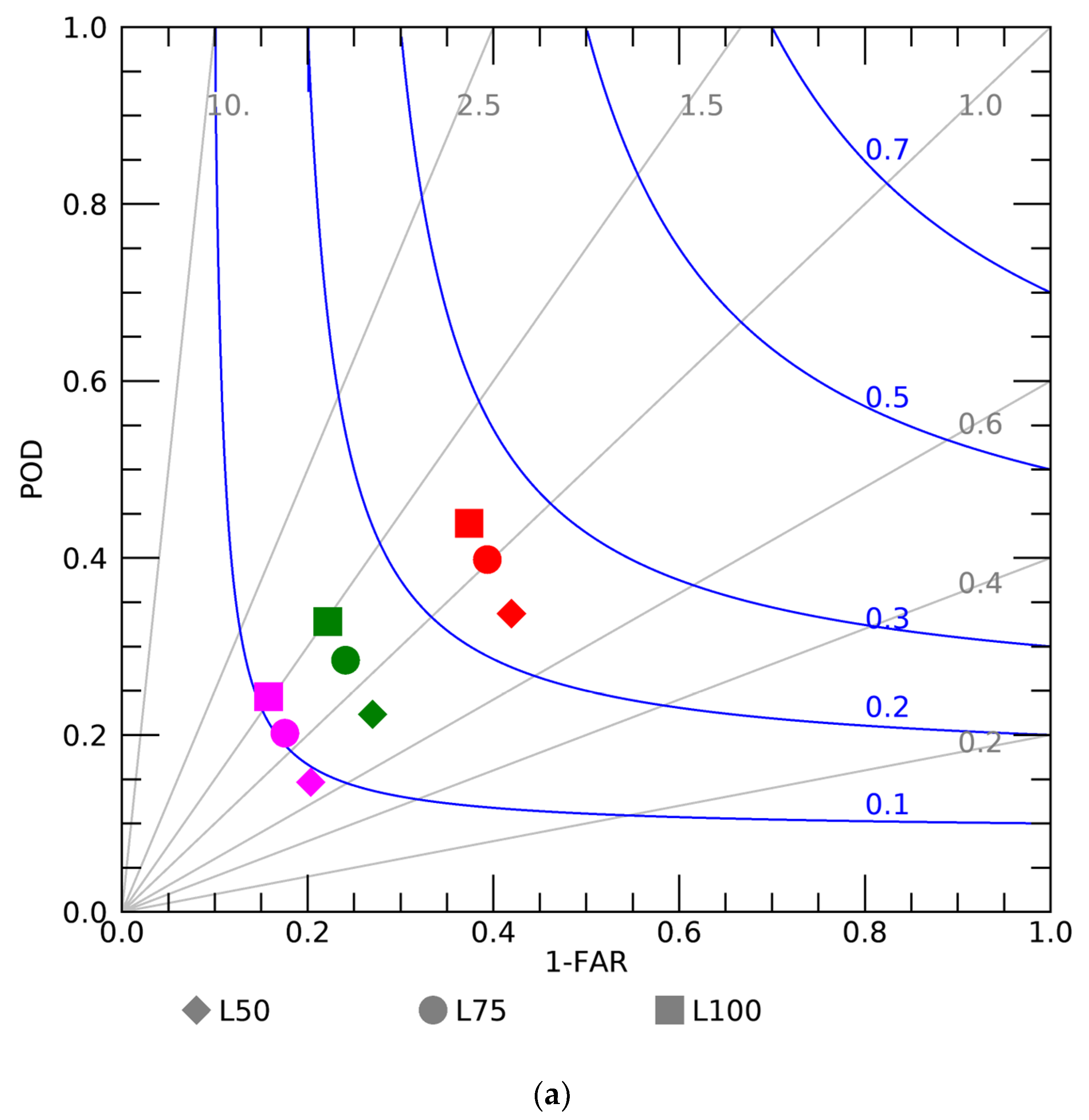
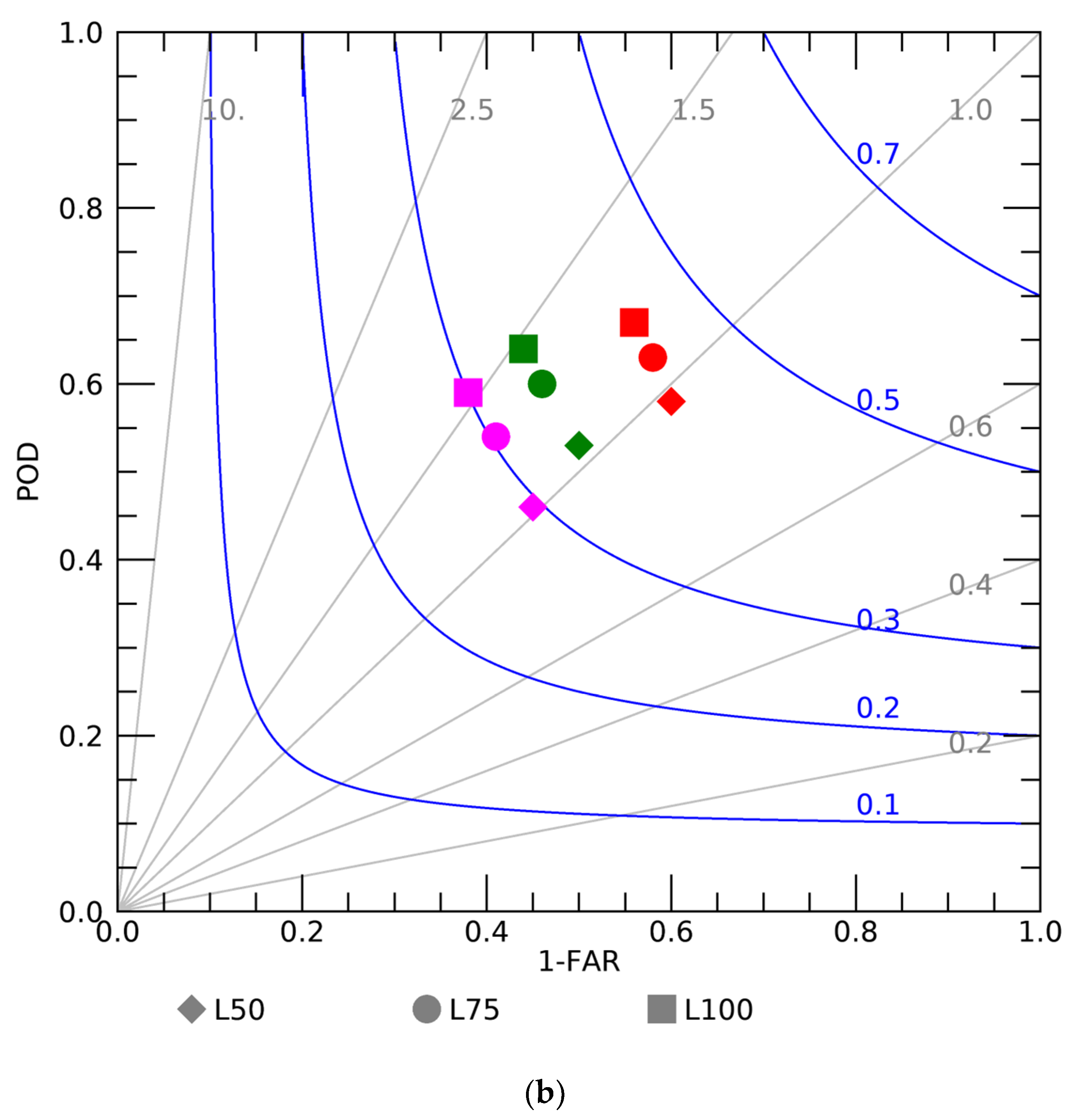
3.2. Comparison among L50, L75, and L100 Configurations and Upscaling of the Model Output

Table 2 shows the number of strokes simulated in different seasons and for the whole year, along with the Pearson correlation coefficient for the time series of daily observed and forecast strokes, both in the different seasons and for the whole year. For the computation of the Pearson correlation coefficient, the pairs used are the daily forecasted total strokes value and the corresponding daily observed value. The histogram in Figure 4 shows the numbers from Table 2 for visual inspection.
Considering the number of strokes for the whole year, it is apparent that the L100 configuration overestimates the number of strokes and L50 underestimates it. L75 gives a very good prediction of the total number of strokes for the whole year.
Considering the forecast behavior for different seasons, we note that L100 overestimates the number of strokes in all seasons, and L50 underestimates the number of strokes in all seasons except winter. All DLS configurations overestimated the strokes in winter. L75 overestimates the strokes in spring, fall, and winter, and underestimates their number in summer. The underestimation in summer is almost compensated by the overestimation in other seasons so that the total number of strokes forecasted by L75 is close to the number of strokes observed for the whole year. The result of this comparison shows that the performance of the DLS settings is dependent on the season. In summer, for example, the number of observed strokes fell between the L75 and L100 configurations, whereas it is between L50 and L75 in spring.
The correlation coefficients for the time series between daily simulated and observed strokes (Table 2) has values around 0.8 or higher for summer, fall, and winter, showing that the WRF model with DLS can predict the day-to-day variability of electric activity over Italy. The correlation coefficient was lower in spring compared to other seasons. The poorer performance of spring compared to other seasons will be further examined in Section 3.3.
Lightning is a manifestation of deep convection, whose characteristics vary with the seasons, and it is expected that a correct prediction of the convective environment would lead to a correct lightning prediction. This subject was investigated, among others, in Lynn [52], who considered the correlation between the fraction skill score (FSS, [90]) of the precipitation forecast and the corresponding score for the lightning forecast, finding a positive correlation for the two scores. Other convective parameters, such as radar reflectivity, could be considered in future studies.
In the remainder of this paper, we consider the statistical scores and analysis that consider the correct positioning of the strokes forecast within the verification domain (Figure 1). As shown in several studies [29,52,91,92], the forecast of lightning and severe weather are difficult tasks because they are typical of convective environments, which are difficult to predict precisely in space and time. The error in lightning forecast occurs because of WRF model errors in simulating convection and errors in the lightning scheme. In addition, most of lightning forecasts are performed using numerical weather prediction models (NWP) with high horizontal resolutions (1–5 km), which gives a more reliable representation of cloud types and structures compared to coarser horizontal resolution models. Nevertheless, the performance of high-resolution models, quantified by some statistical scores, can be worse than that of coarser horizontal resolution models because of the well-known double penalty error [93,94]. For these reasons, it is important to consider the lightning forecast performance not only for the WRF grid cell horizontal resolution (3 km in our case) but also for coarser horizontal resolutions or using scores that consider the neighborhood forecast, i.e., FSS.
In this paper we adopt a simple upscaling technique of the model output, shown in Figure 5. We sum the number of strokes simulated by WRF over an equal number of model grid cells in both horizontal directions. The number of grid cells summed in each direction is referred to as the upscale factor. Upscale factors of 1 (i.e., 3 km WRF grid), 2, 4, 8, and 16 are considered, which correspond to an evaluation of the model performance for grid cells with 3 km to 48 km horizontal dimensions. Figure 5 shows an example of applying an upscale factor of 4 to the WRF 3 km horizontal resolution grid. The horizontal grid spacing of the upscaled grid is 12 km and the grid cell is equivalent to sixteen grid cells in the WRF model.
As stated above, in the following section we show statistics for the daily lightning forecast that consider the position error of the strokes. Of course, upscaling the model output improves these statistics because we neglect a spatial error of d   2 , where d is the grid spacing, which increases for larger grids. Regarding the Department of Civil Protection (DPC), which issues meteorological alerts over Italy, upscaling the model does not limit the practical usefulness of the lightning forecast as all areas corresponding to grid cells from 3 km to 24 km are less than the DPC’s alert areas. For the 48 km grid, there are cases where the alert area is the same size as the upscaled grid.
Figure 6 shows the performance diagram for 6 km and 24 km horizontal grid cells (upscale factors of 2 and 8, respectively). The performance is shown for 1 stroke per grid cell, 10 strokes per grid cell, and 30 strokes per grid cell. For grid sizes, the performance decreases with the number of strokes, which is indicative of the convection intensity. The performance of the 24 km grid cell is better than that of the 6 km grid cell, as expected, because we are neglecting larger spatial errors for larger grid spacing. The frequency bias (FBIAS) of L75 is close to 1 for the 6 km horizontal resolution, whereas the FBIAS of L100 is larger than 1 and the FBIAS of L50 is less than 1. The threat scores (TS) for L100 and L75 have similar values for both 6 km and 24 km, whereas L50 has lower values. There is an increase in the FBIAS for the 24 km grid for all configurations, and L50 has the best FBIAS. In any case, TS is better for L75 and L100 compared to L50.
All in all, the L75 configuration has the best performance because its FBIAS is closer to 1 compared to L100 while having similar TS values, and the TS of L75 is always better than L50. This result is further supported by the number of flashes simulated in different seasons (Figure 4). For these reasons, L75 will be used when showing the performance of the DLS scheme in the following sections.

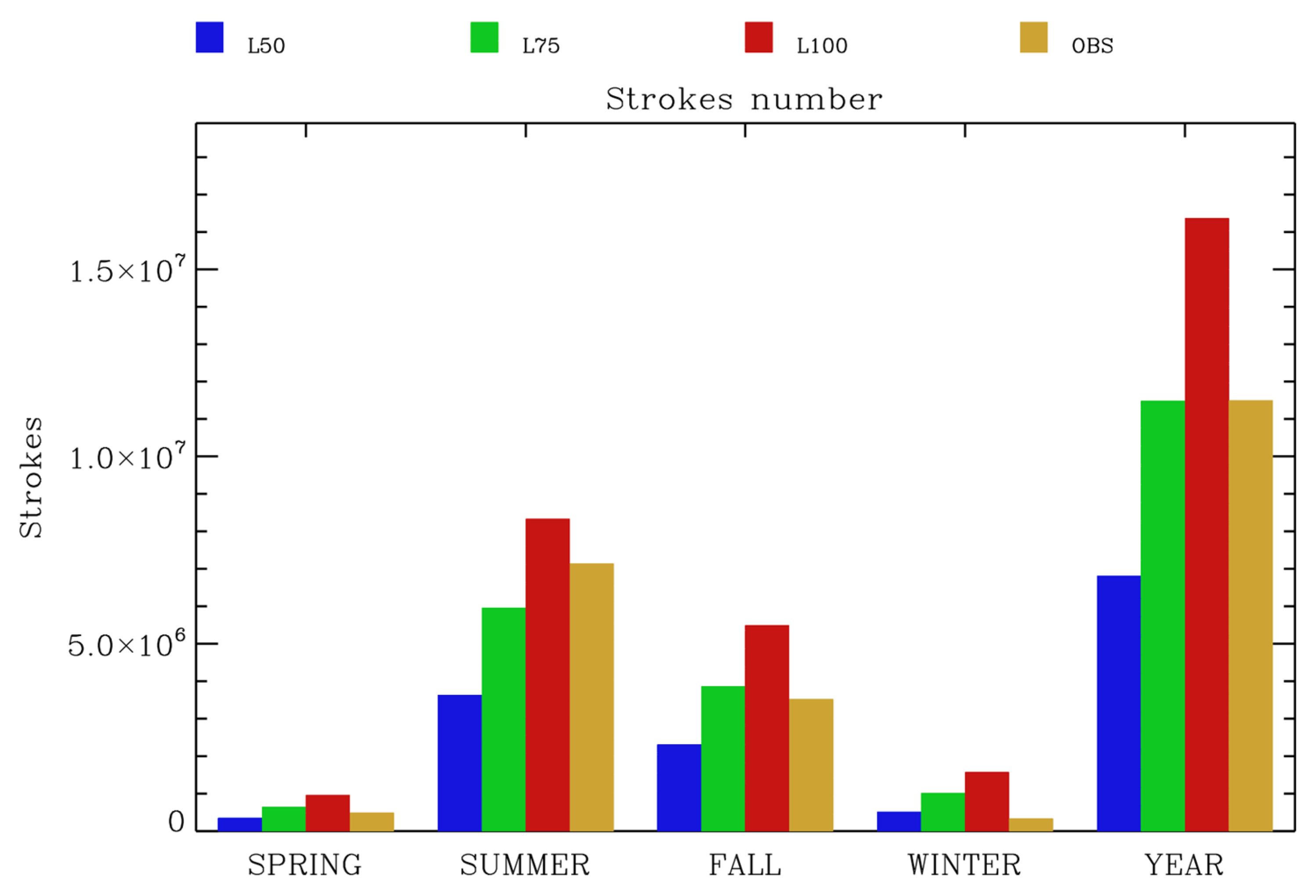
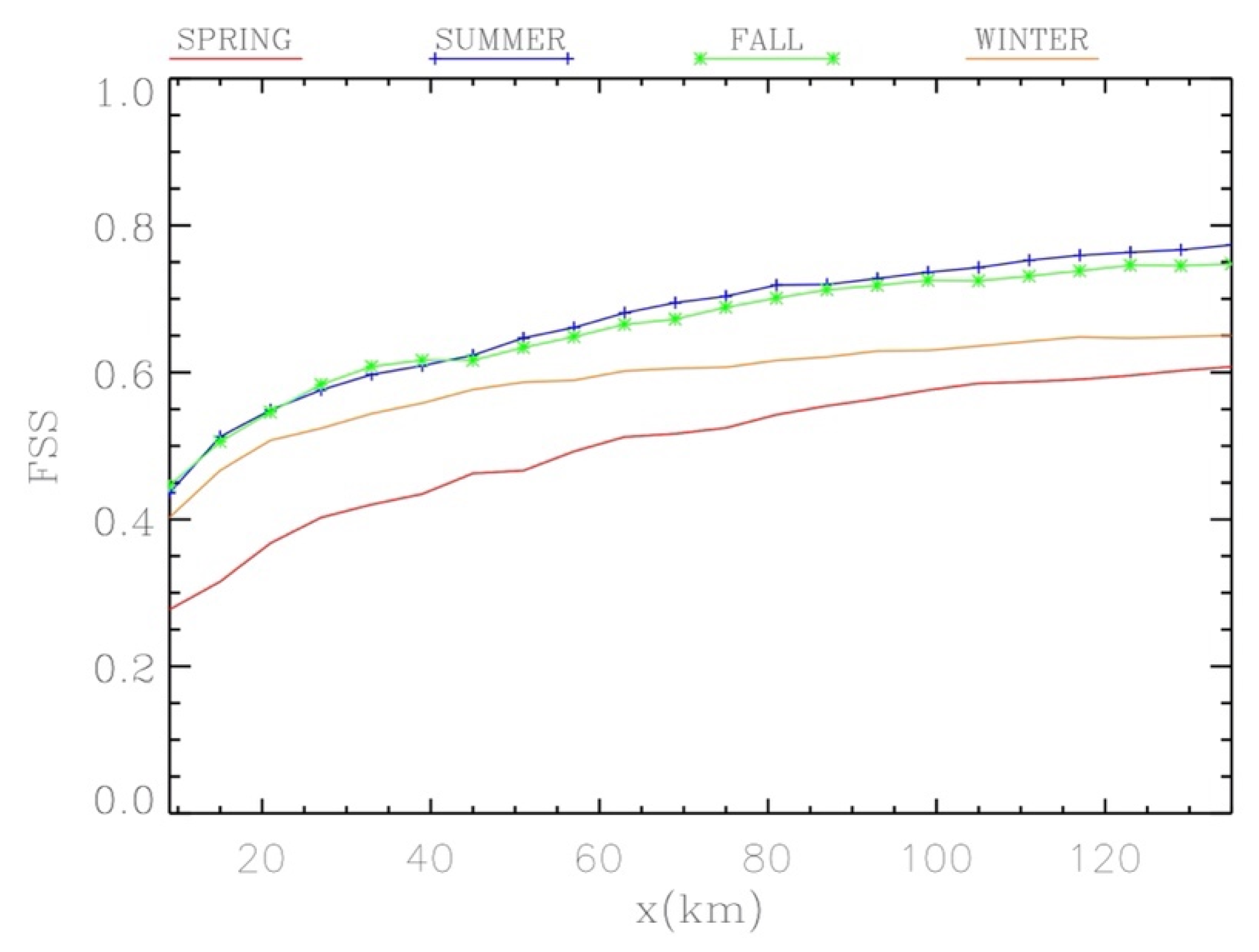
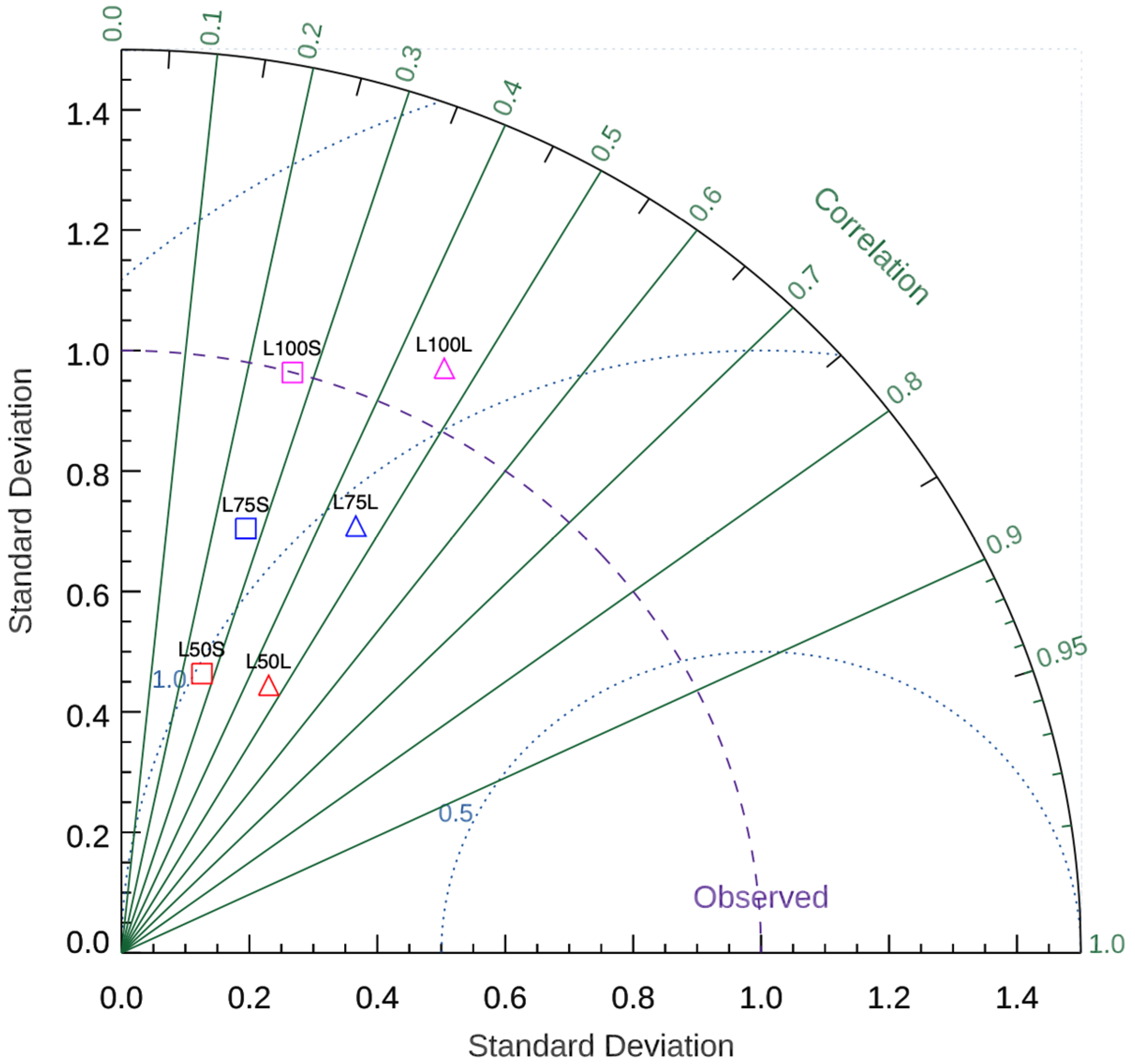
3.3. Performance in Different Seasons and Comparison between the Forecast over Land and over Sea

Because of the high variability of the Mediterranean climate and strokes distribution with seasons, it is important to consider the performance of the DLS in different seasons. This is studied in this section using the fraction skill score (FSS, [90]). This metric is a skill score based on the mean squared error of the forecasts relative to a worst-case reference forecast (see Appendix A for the details). This metric is well suited for evaluating forecasts produced by neighborhood approaches. The forecast is considered skillful for a scale x if FSS is greater than 0.5 + fo/2, where fo is the probability of occurrence of the forecasted event. We consider the event as having at least 1 stroke in a grid cell per day for the L75 configuration of the lightning scheme. The probability of occurrence of the forecast event fo is about 1% in winter and spring, and 2% in summer and fall. These probabilities were estimated considering the number of grid cells in which strokes were observed over the total number of grid cells.
Lynn [52] used a neighborhood approach to verify the lightning forecast made with the same dynamical scheme used here. Forecast probabilities of hourly lightning were evaluated using the method described in [92] and the optimal performance of the lightning forecast was found when the smoothing parameter σ = 48 km. With this length-scale, he computed the saving over climatology (SOC) for different cost to loss ratios as well as other statistics, including FSS (see his Figure 9a). He found (mostly) positive values for SOC for different forecast hours with the exception of the forecast hours from +7 h to +9 h, where negative values were found for cost to loss ratios greater than 0.2–0.25, depending on the forecasting hour. The FSS score was computed for each forecast hour for the length-scale of 48 km, showing a decreasing trend with increasing forecast time. Larger FSS values generally corresponded with larger values for the SOC. Interestingly, for the +9 h forecasting time, he found that the saving over climatology was still positive for a cost to loss ratio less than about 0.2 and for FSS = 0.48. This indicates that forecasts that are not considered useful based on FSS value can have an economic value to some users.
Considering the value of fo for different seasons and the result of Lynn [52], a 0.5 threshold was used to determine the scale of usefulness of the forecast.
The results for different seasons are shown in Figure 7. In summer and fall, FSS is greater than 0.5 at a 15 km length-scale; in winter, FSS is greater than 0.5 at a 21 km length-scale; and in spring, FSS is greater than 0.5 at a 63 km length-scale. Thus, the WRF model and DLS scheme performed better in summer and fall than winter, and the worst FSS score is for spring, highlighting a lower ability to forecast strokes in this season. Possible solutions to improve the lightning forecast, especially in spring, include an ensemble forecast and/or data assimilation at a local scale in a rapid update cycle (RUC) forecasting system (see Discussion for more detail).
The results for the FSS score show that the performance is similar for summer and fall, when the largest number of strokes is observed, followed by winter and finally spring. The FSS becomes greater than 0.5 for spatial scales smaller than the spatial dimensions of the meteorological alert areas used by the Civil Protection Department for summer, fall, and winter. For spring, the forecast becomes useful for scales (about 60 × 60 km2) larger than the meteorological alert areas used by the Civil Protection Department.
Another important point to consider for Italy is the comparison of the performance of the forecast of strokes over land and over sea. This is quantified considering the Taylor diagram for the whole period and a 48 km grid (upscale factor 16). The classification of land and sea grid points was carried out according to the WRF land-sea mask. Thus, when upscaling the forecast, a grid cell is classified as land if the number of land grid cell in the WRF model is greater than the sea grid cells and vice versa. After upscaling the forecast, it turned out that a few (6) grid cells (48 km length) had an equal number of WRF- grid cells labelled as land or sea, which could not be labelled as land or sea, so they were discarded from the analysis. The Taylor diagram is shown in Figure 8.
The results show that the strokes forecast is better over land than over sea for all DLS configurations (L50, L75, L100). The better performance over land the sea is likely caused by the orography, which acts as a triggering mechanism for convection and/or focuses convection on specific regions, effects that are at least partially represented by the WRF. The correlation coefficient is not high (about 0.45 for land grid points and 0.25–0.28 for sea grid points) showing the difficulty of precisely forecasting the position and amount of electrical activity for the following day, as the Taylor diagram considers both aspects of the strokes forecast. The low value of the correlation coefficient is expected because it is difficult to precisely predict convection one day in advance. Indeed, convection often develops on a small scale, usually embedded in larger scale meteorological systems, and sometimes, especially in summer, as a local phenomenon. Small meteorological systems are inherently difficult to predict one day in advance [11,36,44,95,96] and the correlation coefficient is expected to be low because lightning is a manifestation of a small-scale phenomenon.
The standard deviation of the observations is better represented by the L100 configuration, especially over the sea, whereas L75 and (especially) L50 underestimates the standard deviation of the observations both over land and sea. Similar results were obtained for smaller upscale factors; however, the value of the correlation decreases as the grid cell dimension decrease. For example, the correlation for the 24 km grid cell is about 0.35 for the land and 0.2 for the sea.

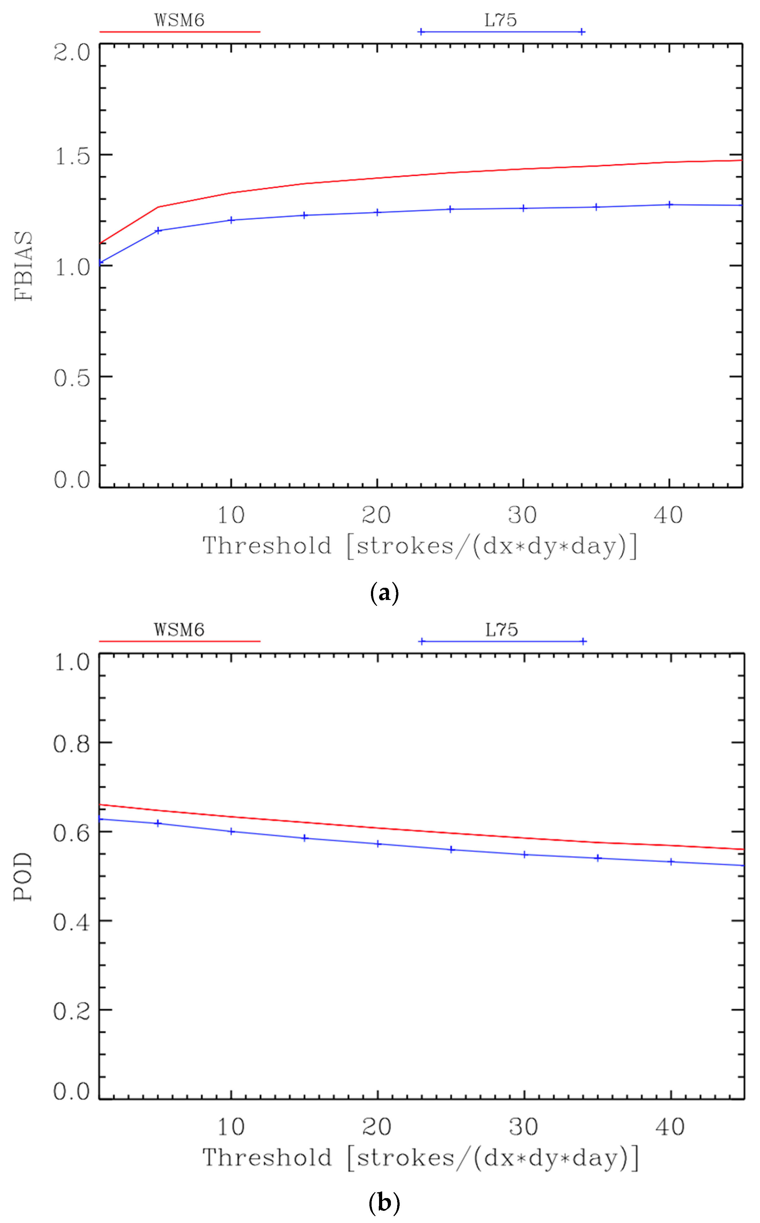
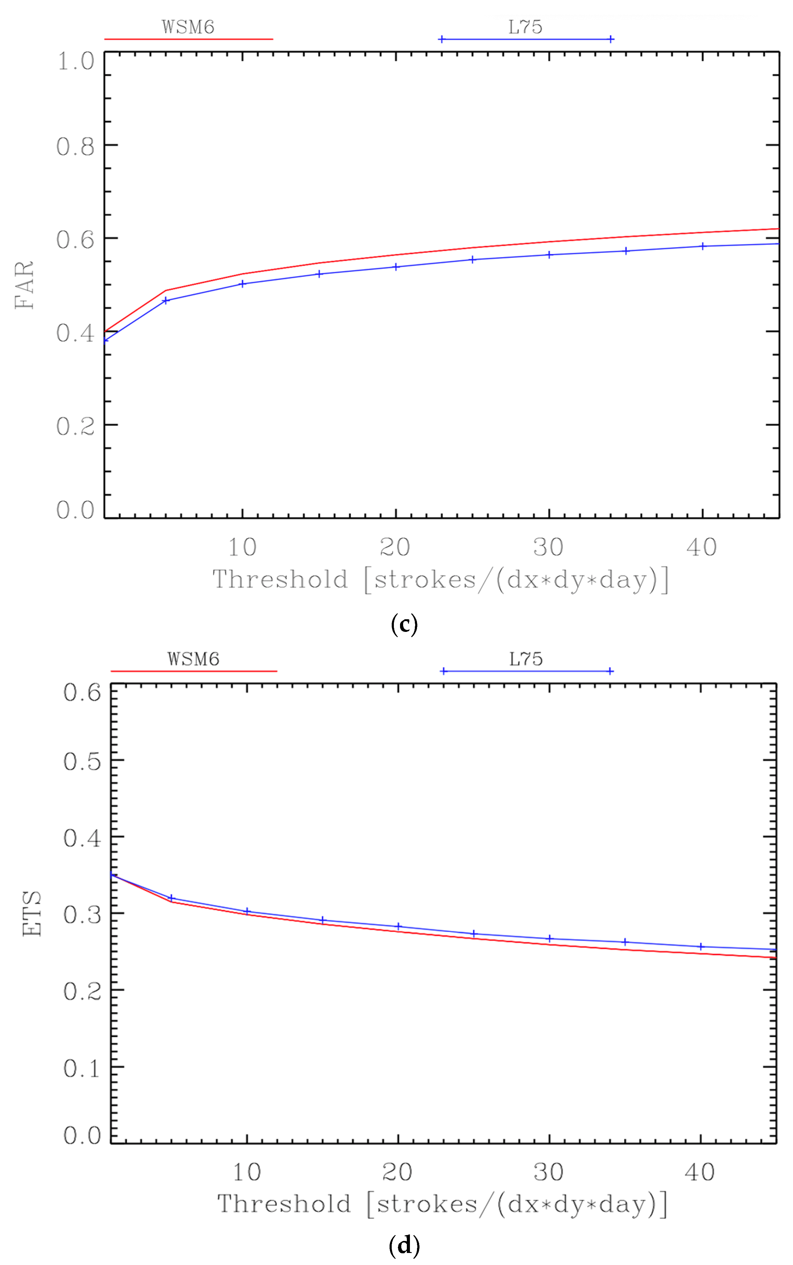
3.4. Sensitivity to the Microphysical Scheme

The electric potential and energy computed by the DLS depends on the hydrometeor mixing ratios (liquid water, graupel, snow, and ice), thus changing the microphysical scheme plays a major role in the lightning forecast. For this reason, we studied the sensitivity of the strokes forecast to the microphysical scheme by simulating the fall cases (46 cases) with the WSM6 microphysical scheme. This scheme and the Thompson scheme were chosen because they are both used by the DPC through agreements with CNR-ISAC and CIMA Foundation. The charge transferred in 1 s within the cloud is 0.75 × 10⁻⁴ C, so the impact of changing the microphysical scheme can be quantified by comparing WSM6 and L75 forecasts.
The results are shown for 24 km grid cells, but similar conclusions were found for other grid spacings. Comparing the FBIAS for the two different configurations, WSM6 produced higher values for all thresholds, showing that the WSM6 microphysical scheme predicts more convection compared to the Thompson scheme [97,98]. The larger FBIAS of the WSM6 configuration results in both larger POD and FAR scores than the Thompson scheme for all of the thresholds considered. The ETS score improves for higher POD and worsens for higher FAR, so the ETS of WSM6 and L75 are similar (Figure 9d). The results of this experiment show an important sensitivity of the forecast of strokes to the choice of the microphysical scheme used in the WRF, as expected. The L75 configuration is preferred in this work because of the tendency of WSM6 to overestimate convection, as shown by the FBIAS cores, and because the ETS score is slightly better for L75.
It is important to highlight that the scope of this test is to show how sensitive stroke prediction can be to a change in the microphysical scheme rather than developing a complete sensitivity test. The impact of changing the microphysical scheme on stroke prediction should be considered in other seasons, as microphysical regimes may vary among seasons so that results of the sensitivity test can be different. A full developed sensitivity test is beyond the scope of this paper, so the analysis in this section is only a preliminary study of the problem.

4. Discussion

In this paper, we applied the dynamic lightning scheme of Lynn et al. [72] to the WRF model for a year-long lightning forecast over Italy. A total of 162 days were considered, accounting for most of the strokes that occurred during the year and throughout the different seasons and times of the day. The forecast is issued for the next day using a WRF model configuration at 3 km horizontal resolution and 50 vertical levels.
Three different configurations of the lightning dynamic scheme were considered: L50, as in Lynn et al. [72], L75, and L100. These configurations differ for the key parameter of assumed charge transferred in one second within convective and stratiform clouds.
Among the three dynamic lightning scheme configurations considered, L75 accurately forecast the total number of strokes recorded in all cases, whereas L50 underestimated and L100 overestimated the number of strokes. However, the relative performance of L50, L75, and L100 for the number of strokes depended on the season. The time-series correlation of daily observed and forecasted strokes over the domain (6°E–19°E; 36.5°N–47°N) was around 0.75, depending on the season, with the largest value in winter (around 0.85) and the lowest in spring (around 0.65).
Qualitative scores (FBIAS, ETS, POD, FAR) computed for the 3 km grid and different strokes thresholds (from 1 stroke per grid cell per day to 45 strokes per grid cell per day) had low values, and upscaling of the model output by summing the forecast and observed strokes over grids with larger grid sizes (from 6 to 48 km), improved the results as spatial errors became smaller than the grid size. Upscaling does not limit the practical usefulness of the forecast, given that the meteorological alert areas used by the Department of Civil Protection have typical dimensions of 50 km by 50 km. Among the different configurations of the DLS, L75 performed slightly better. However, L50, L75, and L100 showed very similar spatial patterns for the predicted strokes, the main difference being the number of strokes simulated by each configuration.
The analysis of the fraction skill score showed that the best lightning forecast was for summer, followed by fall, winter, and spring. For spring, the forecast usefulness started at scales of around 60 km for a 1 stroke per grid cell per day event, which is larger than those used by the Civil Protection Department to issue meteorological alerts, so the forecast performance in this season is not satisfactory. For other seasons, the forecast is useful at scales well below those used by the Civil Protection Department to issue meteorological alerts. Future studies will consider the point of improving the lightning forecast, especially in spring. An important technique to improve the convective environments forecast is the use of data assimilation at the local scale in rapid update data assimilation/forecast cycles [99]. Among the local data, lightning plays a major role [29,30,32,52,100,101] and a study is underway to show the impact of lightning data assimilation on the strokes forecast. A further enhancement of the accuracy of convective cell prediction can be obtained by exploiting ensemble predictions, which have a long tradition in meteorology (see, for instance [102,103]) and has been adopted as a standard procedure by various meteorological agencies [104]. The lightning forecast could take advantage of ensemble forecasting by quantifying the predictability of convective events through the ensemble spread and by removing the most unpredictable components of the weather forecast through the ensemble mean. However, the use of the ensemble for lightning forecast needs considerable computing resources because of the high horizontal resolutions required to simulate flashes.
The lightning forecast performance varied between the sea and the land, where the analysis of the Taylor diagram showed a better performance over land than sea. This result is likely caused by a better WRF simulation of convection over land, where the effect of topography may trigger/focus the convection over specific areas.
Finally, the sensitivity of the strokes forecast to changing the microphysical parameterization scheme was investigated for a specific microphysics scheme. We considered the comparison between the WSM6 one-moment microphysics scheme and the Thompson microphysics scheme, which are both used in forecasting systems by the DPC. Results showed a better performance of the Thompson scheme in terms of FBIAS and FAR scores, whereas the POD was better for the WSM6 microphysics scheme. Minor differences were found for ETS, with the Thompson scheme performing slightly better. These results show that DLS performance is sensitive to the choice of the microphysics scheme, and the WSM6 scheme predicts more flashes compared to Thompson [97,98].

5. Conclusions

All in all, the results of this study show that the dynamic lightning scheme of Lynn et al. [72] can be applied with success over Italy for a next day strokes forecast, although careful calibration of the scheme is needed to produce better forecasts. The forecast quality depends on the season, spatial scales, and surface type.

Author Contributions

Conceptualization, S.F., B.H.L., S.D. and R.C.T.; methodology, S.F. and B.H.L., software, R.C.T. and S.F.; validation, M.L., R.C.T., B.H.L., S.P. and S.F.; data curation, S.F. and R.C.T.; writing—original draft preparation, S.F. and R.C.T.; writing—review and editing, B.H.L., S.P., M.L. and S.D.; funding acquisition, S.F. All authors have read and agreed to the published version of the manuscript.

Funding

This work was carried out within the framework of the AEROMET project funded by the Lazio Region government (contract n. A0375-2020-36588—“Progetti di Gruppi di Ricerca 2020” LazioInnova—FESR Fondo Europeo di Sviluppo Regionale Programma Operativo regionale del Lazio).

Data Availability Statement

LINET data can be acquired from Nowcast GmbH (https://www.nowcast.de/, accessed on 1 July 2022). Simulated flashes data can be requested from the corresponding author.

Acknowledgments

ECMWF is acknowledged for providing the computational resources through the project SPITFEDE as well as for providing initial and boundary conditions for WRF simulations. LINET data were provided by Nowcast GmbH (https://www.nowcast.de/, accessed on 1 July 2022) within a scientific agreement between H.D. Betz and the Satellite Meteorological Group of CNR-ISAC in Rome.

Conflicts of Interest

The authors declare no conflict of interest.

Appendix A

The forecast verification was assessed by several metrics. In this appendix, those statistics are briefly introduced. The Pearson (ordinary) correlation coefficient gives a measure of the association between two variables x and y [105]:
r x y = [ 1 / ( n 1 ) ] i = 1 n [ ( x i x ¯ ) ( y i y ¯ ) ] [ 1 / ( n 1 ) ] i = 1 n ( x i x ¯ ) 2 [ 1 / ( n 1 ) ] i = 1 n ( y i y ¯ ) 2
where the bar is the average value of the variable computed over the sample size n.
Scores from 2 × 2 dichotomous contingency tables (Table A1) are used to quantify the model performance. Scores are computed for different lightning density threshold values (the event): 1 stroke per grid cell per day, from 5 to 45 strokes per grid cell per day, and every 5 strokes per grid cell per day.
Table A1. Elements of the contingency table.
ObservedObserved
YESNO
ForecastYESab
ForecastNOcd
In particular, defining the hits (a, when both the forecast and the corresponding observation are above or equal to a threshold value), false alarms (b, when the forecast is above or equal to a threshold value while the corresponding observation is below the threshold value), misses (c, when the forecast is below a threshold value while the corresponding observation is above or equal to the threshold value), and correct no forecast (d, when both the forecast and the corresponding observation are below a threshold value). Starting with the elements in the contingency tables, summed over all the cases of the specific analysis considered, the following scores are calculated:
FBIAS = a + b a + c
POD = a a + c
TS = a a + b + c
ETS = a a r a + b + c a r ,   a r = ( a + b ) ( a + c ) a + b + c + d
FAR = b a + b
where ar is the probability of a correct forecast by chance when the yes/no forecast occurrence is independent from the observation. The frequency bias (FBIAS; range (0, +∞), where 1 is the perfect score, i.e., when no misses and false alarms occur) is the ratio of the number of yes forecasts of the event and the observed number of yes events. The probability of detection (POD; range (0, 1), where 1 is the perfect score and 0 is the worst value) is the proportion of correct forecasts over the total number of observed events. The threat score (TS; range (0, 1), where 1 is the perfect score and 0 is the worst score) is the number of correct forecasts of the event divided by the total number of occasions on which the event was observed and/or forecast. The equitable threat score (ETS; range (−1/3, 1), where 1 is the perfect score and 0 is a useless forecast) is the proportion of correct forecasts corrected for the probability of a correct forecast by chance, where the occurrence/non-occurrence of the event is independent from its observation.
The FAR (false alarm rate; range (0, 1), where 0 is the best forecast and 1 represents the worst forecast) is that proportion of forecasted events that fail to materialize.
A performance diagram (Figure 6 of the paper) is used to graphically represent the performance given by most of the above scores. The x-axis of the performance diagram shows the success ratio (1-FAR), and POD is along the y-axis. Different values for FBIAS lie on straight lines from the axes origin and are represented as grey lines. Different values for the threat score are represented by hyperboles in the performance diagram and are represented as blue lines. The model performance, quantified by the scores of a contingency table, is represented as a single point in the performance diagram.
The fraction skill score (FSS, [90]) is based on the mean squared error (MSE) of the forecast relative to the worst case. It is especially suited for verifications considering the neighborhood approach. It is given by:
FSS ( n ) = MSE ( n ) MSE ( n ) , r e f MSE ( n ) , p e r f e c t MSE ( n ) , r e f = 1 MSE ( n ) MSE ( n ) , r e f
where the MSE is given by:
MSE ( n ) = 1 N x N y i = 1 N x j = 1 N y [ O ( n ) , i , j M ( n ) , i , j ] MSE ( n ) , r e f = 1 N x N y [ i = 1 N x j = 1 N y O 2 ( n ) , i , j + i = 1 N x j = 1 N y M 2 ( n ) , i , j ]
In the above equations, Nx and Ny are the number of grid points in the x and y directions (635 in both directions in this paper). Fractions are generated for different spatial scales by changing the value of n, which can be any odd value up to 2N − 1, where N is the number of points along the longest side of the domain. In the statistics of this paper, n varies from 3 to 43, corresponding to spatial scales from 9 to 129 km. The FSS score is summed over all grid points in the domain, and it is defined such that the perfect (no) skill forecast has an FSS equal to 1 (0).
O(n),i,j is the resultant field of observed fractions for a square of length n obtained from the binary field Io and M(n),i,j is the resultant field of forecast fractions for a square of length n obtained from the binary field IM. Specifically, Io (IM) is 1 if the observed (forecast) lightning density per grid cell is above a threshold value, and Io (IM) is 0 if the observed (forecast) lightning density per grid cell is below this threshold. The corresponding formulae are as follows:
O ( n ) , i , j = 1 n 2 k = 1 n l = 1 n I O [ i + k 1 ( n 1 ) 2 , j + l 1 ( n 1 ) 2 ]
M ( n ) , i , j = 1 n 2 k = 1 n l = 1 n I M [ i + k 1 ( n 1 ) 2 , j + l 1 ( n 1 ) 2 ]
The Taylor diagram [106] provides a way of graphically summarizing how closely a pattern matches observations. The similarity between two patterns (forecast and observed daily lightning density) is quantified in terms of their correlation, their centered root mean square difference, and the amplitude of their variations (represented by their standard deviations). These diagrams are useful in evaluating the relative skill of different models. In this research, the Taylor diagram is used to quantify the relative skill of the prediction of strokes over land and over sea. Model root mean square errors and standard deviations are divided by the observation standard deviation for the graphical representation (see Figure 9). The distance of each point, which quantifies the statistics for each model, from the axes origin is the standard deviation of the model and values can be read on the x- or y-axis (a value of 1 means that the standard deviation of the model is equal to the standard deviation of the observations); the Pearson correlation coefficient for the model and observations is measured by the angle along the circumference arc (values are given in the outer circumference in Figure 9), and the centered root mean square difference between the model and observations is given by the radius of the dotted blue circumference corresponding to the model point. The centered root mean square difference is represented as units of observed standard deviation, and a value of 1 means that the centered root mean square difference is equal to the observation standard deviation. The best performance of the model is when the point representing the model statistics lies on the x-axis at the abscissa 1.

References

  1. American Meteorological Society. Lightning explodes dynamite. Mon. Weakly Rev. 1924, 52, 313. [Google Scholar] [CrossRef]
  2. American Meteorological Society. Loss of forty-seven head of cattle by a single lightning bolt. Mon. Weakly Rev. 1924, 52, 452. [Google Scholar] [CrossRef]
  3. Lopez, R.E.; Holle, R.L. Fluctuations of lightning casualties in the United States: 1959–1990. J. Clim. 1996, 9, 608–615. [Google Scholar] [CrossRef] [Green Version]
  4. Lopez, R.E.; Heitkamp, T.A. Lightning casualties and property damage in Colorado from 1950 to 1991 based on Storm Data. Weather Forecast. 1995, 10, 114–126. [Google Scholar] [CrossRef] [Green Version]
  5. Rorig, M.L.; Ferguson, S.A. The 2000 fire season: Lightning-caused fires. J. Appl. Meteorol. 2002, 41, 786–791. [Google Scholar] [CrossRef]
  6. Holle, R.L.; López, R.E.; Arnold, L.J.; Endres, J. Insured lightning-caused property damage in three western states. J. Appl. Meteorol. 1996, 35, 1344–1351. [Google Scholar] [CrossRef] [Green Version]
  7. Hodanish, S.; Holle, R.; Lindsey, D.T. A small updraft producing a fatal lightning flash. Weather Forecast. 2004, 19, 627–632. [Google Scholar] [CrossRef] [Green Version]
  8. Holle, R.L.; López, R.E.; Navarro, B.C. Deaths, injuries, and damages from lightning in the United States in the 1890s in comparison with the 1990s. J. Appl. Meteorol. 2005, 44, 1563–1573. [Google Scholar] [CrossRef] [Green Version]
  9. Ashley, W.S.; Gilson, C.W. A reassessment of U.S. lightning mortality. Bull. Am. Meteorol. Soc. 2009, 90, 1501–1518. [Google Scholar] [CrossRef]
  10. Wallmann, J.; Milne, R.; Smallcomb, C.; Mehle, M. Using the 21 June 2008 California lightning outbreak to improve dry lightning forecast procedures. Weather Forecast. 2010, 25, 14471462. [Google Scholar] [CrossRef]
  11. Schultz, C.J.; Petersen, W.A.; Carey, L.D. Preliminary development and evaluation of lightning jump algorithms for the real-time detection of severe weather. J. Appl. Meteorol. Climatol. 2009, 48, 2543–2563. [Google Scholar] [CrossRef] [Green Version]
  12. Koshak, W.J.; Cummins, K.L.; Buechler, D.E.; Vant-Hull, B.; Blakeslee, R.J.; Williams, E.R.; Peterson, H.S. Variability of CONUS lightning in 2003–2012 and associated impacts. J. Appl. Meteorol. Climatol. 2015, 54, 15–41. [Google Scholar] [CrossRef] [Green Version]
  13. Epicentro—Istituto Superiore di Sanità. Available online: www.epicentro.iss.it/fulmini/epidemiologia (accessed on 3 June 2022).
  14. Mäkelä, A.; Saltikoff, E.; Julkunen, J.; Juga, I.; Gregow, E.; Niemelä, S. Cold-season thunderstorms in Finland and their effect on aviation safety. Bull. Am. Meteorol. Soc. 2013, 94, 847–858. [Google Scholar] [CrossRef]
  15. Mazur, V.; Fisher, B.D.; Gerlach, J.C. Lightning strikes to a NASA airplane penetrating thunderstorms at low altitudes. J. Aircr. 1986, 23, 499–505. [Google Scholar] [CrossRef]
  16. Sweers, G.; Birch, B.; Gokcen, J. Lightning Strikes: Protection, Inspection, and Repair. Aero. 2012. Available online: https://www.boeing.com/commercial/aeromagazine/articles/2012_q4/4/ (accessed on 3 June 2022).
  17. Rash, C.E. When lightning strikes. AeroSaf. World 2010, 5, 18–23. [Google Scholar]
  18. Parodi, A.; Mazzarella, V.; Milelli, M.; Lagasio, M.; Realini, E.; Federico, S.; Torcasio, R.C.; Kerschbaum, M.; Llasat, M.C.; Rigo, T.; et al. A Nowcasting Model for Severe Weather Events at Airport Spatial Scale: The Case Study of Milano Malpensa. SIDs (SESAR Innovation Days). 2021. Available online: https://www.researchgate.net/profile/Riccardo-Biondi-2/project/SINOPTICA-H2020/attachment/61d353a4b3729f0f619eaa4f/AS:1108251361972224@1641239123907/download/SID_SINOPTICA_paper_final_revision.pdf?context=ProjectUpdatesLog (accessed on 3 June 2022).
  19. Goodman, S.J.; MacGorman, D.R. Cloud-to-ground lightning activity in mesoscale convective complexes. Mon. Weakly Rev. 1986, 114, 2320–2328. [Google Scholar] [CrossRef] [Green Version]
  20. Kane, R.J. Correlating lightning to severe local storms in the northeastern United States. Weather Forecast. 1991, 6, 3–12. [Google Scholar] [CrossRef] [Green Version]
  21. Smith, J.A.; Baeck, M.L.; Morrison, J.E.; Sturdevant-Rees, P. Catastrophic rainfall and flooding in Texas. J. Hydrometeorol. 2000, 1, 5–25. [Google Scholar] [CrossRef]
  22. McCaul, E.W.; Buechler, D.E.; Goodman, S.J.; Cammarata, M. Doppler radar and lightning network observations of a severe outbreak of tropical cyclone tornadoes. Mon. Weakly Rev. 2004, 132, 1747–1763. [Google Scholar] [CrossRef] [Green Version]
  23. Underwood, S.J. Cloud-to-ground lightning flash parameters associated with heavy rainfall alarms in the Denver, Colorado, Urban Drainage and Flood Control District ALERT Network. Mon. Weakly Rev. 2006, 134, 2566–2580. [Google Scholar] [CrossRef]
  24. Gatlin, P.N.; Goodman, S.J. A total lightning trending algorithm to identify severe thunderstorms. J. Atmos. Ocean. Technol. 2010, 27, 3–22. [Google Scholar] [CrossRef]
  25. Rudlosky, S.D.; Fuelberg, H.E. Documenting storm severity in the mid-Atlantic region using lightning and radar information. Mon. Weakly Rev. 2013, 141, 3186–3202. [Google Scholar] [CrossRef]
  26. Chronis, T.; Carey, L.D.; Schultz, C.J.; Schultz, E.V.; Calhoun, K.M.; Goodman, S.J. Exploring lightning jump characteristics. Weather Forecast. 2015, 30, 23–37. [Google Scholar] [CrossRef] [Green Version]
  27. Christian, H.J.; Blakeslee, R.J.; Boccippio, D.J.; Boeck, W.L.; Buechler, D.E.; Driscoll, K.T.; Goodman, S.J.; Hall, J.M.; Koshak, W.J.; Mach, D.M.; et al. Global frequency and distribution of lightning as observed from space by the Optical Transient Detector. J. Geophys. Res. 2003, 108, ACL 4-1–ACL 4-15. [Google Scholar] [CrossRef]
  28. Holle, R.L.; Said, R.K.; Brooks, W.A. Monthly GLD360 lightning percentages by continent. In Proceedings of the 7th International Lightning Meteorology Conference, Fort Lauderdale, FL, USA, 12–15 March 2018. [Google Scholar]
  29. Fierro, A.O.; Mansell, E.R.; Ziegler, C.L.; MacGorman, D.R. Application of a lightning data assimilation technique in the WRF-ARW Model at cloud-resolving scales for the tornado outbreak of 24 May 2011. Mon. Weakly Rev. 2012, 140, 2609–2627. [Google Scholar] [CrossRef]
  30. Torcasio, R.C.; Federico, S.; Comellas Prat, A.; Panegrossi, G.; D’Adderio, L.P.; Dietrich, S. Impact of lightning data assimilation on the short-term precipitation forecast over the Central Mediterranean Sea. Remote Sens. 2021, 13, 682. [Google Scholar] [CrossRef]
  31. Lynn, B.H.; Kelman, G.; Ellrod, G. An evaluation of the efficacy of using observed lightning to improve convective lightning forecasts. Weather Forecast. 2015, 30, 405–423. [Google Scholar] [CrossRef]
  32. Lai, A.; Gao, J.; Koch, S.E.; Wang, Y.; Pan, S.; Fierro, A.O.; Cui, C.; Min, J. Assimilation of radar radial velocity, reflectivity, and pseudo–water vapor for convective-scale NWP in a variational framework. Mon. Weakly Rev. 2019, 147, 2877–2900. [Google Scholar] [CrossRef]
  33. Roberts, R.D.; Rutledge, S. Nowcasting storm initiation and growth using GOES-8 and WSR-88D data. Weather Forecast. 2003, 18, 562–584. [Google Scholar] [CrossRef] [Green Version]
  34. Wilson, J.W.; Ebert, E.E.; Saxen, T.R.; Roberts, R.D.; Mueller, C.K.; Sleigh, M.; Pierce, C.E.; Seed, A. Sydney 2000 Forecast Demonstration Project: Convective storm nowcasting. Weather Forecast. 2004, 19, 131–150. [Google Scholar] [CrossRef]
  35. Sieglaff, J.M.; Cronce, L.M.; Feltz, W.F.; Bedka, K.M.; Pavolonis, M.J.; Heidinger, A.K. Nowcasting convective storm initiation using satellite-based box-averaged cloud-top cooling and cloud-type trends. J. Appl. Meteorol. Climatol. 2011, 50, 110–126. [Google Scholar] [CrossRef]
  36. Mecikalski, J.R.; Williams, J.K.; Jewett, C.P.; Ahijevych, D.; LeRoy, A.; Walker, J.R. Probabilistic 0–1-h convective initiation nowcasts that combine geostationary satellite observations and numerical weather prediction model data. J. Appl. Meteorol. Climatol. 2015, 54, 1039–1059. [Google Scholar] [CrossRef] [Green Version]
  37. Rossi, P.J.; Chandrasekar, V.; Hasu, V.; Moisseev, D. Kalman filtering–based probabilistic nowcasting of object-oriented tracked convective storms. J. Atmos. Ocean. Technol. 2015, 32, 461–477. [Google Scholar] [CrossRef]
  38. La Fata, A.; Amato, F.; Bernardi, M.; D’Andrea, M.; Procopio, R.; Fiori, E. Horizontal grid spacing comparison among Random Forest algorithms to nowcast Cloud-to-Ground lightning occurrence. Stoch Environ. Res. Risk Assess 2022. [Google Scholar] [CrossRef]
  39. Stern, A.D.; Brady, R.H.; Moore, P.D.; Carter, G.M. Identification of aviation weather hazards based on the integration of radar and lightning data. Bull. Am. Meteorol. Soc. 1994, 75, 2269–2280. [Google Scholar] [CrossRef] [Green Version]
  40. MacGorman, D.R.; Rust, W.D. The Electrical Nature of Storms; Oxford University Press: Oxford, MI, USA, 1998. [Google Scholar]
  41. Short, D.A.; Sardonia, J.E.; Lambert, W.C.; Wheeler, M.M. Nowcasting thunderstorm anvil clouds over Kennedy Space Center and Cape Canaveral Air Force Station. Weather Forecast. 2004, 19, 706–713. [Google Scholar] [CrossRef] [Green Version]
  42. Price, C. Lightning sensors for observing, tracking and nowcasting severe weather. Sensors 2008, 8, 157–170. [Google Scholar] [CrossRef] [PubMed] [Green Version]
  43. Saxen, T.R. The operational mesogammascale analysis and forecast system of the U.S. Army Test and Evaluation Command. Part IV: The White Sands Missile Range Auto Nowcast system. J. Appl. Meteorol. Climatol. 2008, 47, 1123–1139. [Google Scholar] [CrossRef] [Green Version]
  44. Kohn, M.; Galanti, E.; Price, C.; Lagouvardos, K.; Kotroni, V. Nowcasting thunderstorms in the Mediterranean region using lightning data. Atmos. Res. 2011, 100, 489–502. [Google Scholar] [CrossRef]
  45. Dahl, J.M.L.; Höller, H.; Schumann, U. Modeling the flash rate of thunderstorms. Part I: Framework. Mon. Weakly Rev. 2011, 139, 3093–3111. [Google Scholar] [CrossRef] [Green Version]
  46. Hondl, K.D.; Eilts, M.D. Doppler radar signatures of developing thunderstorms and their potential to indicate the onset of cloud-to-ground lightning. Mon. Weakly Rev. 1994, 122, 1818–1836. [Google Scholar] [CrossRef] [Green Version]
  47. Gremillion, M.S.; Orville, R.E. Thunderstorm characteristics of cloud-to-ground lightning at the Kennedy Space Center, Florida: A study of lightning initiation signatures as indicated by the WSR-88D. Weather Forecast. 1999, 14, 640–649. [Google Scholar] [CrossRef]
  48. Yang, Y.H.; King, P. Investigating the potential of using radar echo reflectivity to nowcast cloud-to-ground lightning initiation over southern Ontario. Weather Forecast. 2010, 25, 12351248. [Google Scholar] [CrossRef]
  49. Mosier, R.M.; Schumacher, C.; Orville, R.E.; Carey, L.D. Radar nowcasting of cloud-to-ground lightning over Houston, Texas. Weather Forecast. 2011, 26, 199–212. [Google Scholar] [CrossRef]
  50. Seroka, G.N.; Orville, R.E.; Schumacher, C. Radar nowcasting of total lightning over the Kennedy Space Center. Weather Forecast. 2012, 27, 189–204. [Google Scholar] [CrossRef] [Green Version]
  51. Walker, J.R.; MacKenzie, W.M., Jr.; Mecikalski, J.R.; Jewett, C.P. An enhanced geostationary satellite–based convective initiation algorithm for 0–2-h nowcasting with object tracking. J. Appl. Meteorol. Climatol. 2012, 51, 1931–1949. [Google Scholar] [CrossRef]
  52. Lynn, B.H. The Usefulness and Economic Value of Total Lightning Forecasts Made with a Dynamic Lightning Scheme Coupled with Lightning Data Assimilation. Weather Forecast. 2017, 32, 645–663. [Google Scholar] [CrossRef]
  53. Solomon, R.; Baker, M. A one-dimensional lightning parameterization. J. Geophys. Res. 1996, 101, 14983–14990. [Google Scholar] [CrossRef]
  54. Solomon, R.; Medaglia, C.M.; Adamo, C.; Dietrich, S.; Mugnai, A.; Biader Ceipidor, U. An explicit microphysics thunderstorm model. Int. J. Model. Simul. 2005, 25, 112–118. [Google Scholar] [CrossRef]
  55. Mansell, E.R.; MacGorman, D.R.; Ziegler, C.L.; Straka, J.M. Simulated three-dimensional branched lighting in a numerical thunderstorm model. J. Geophys. Res. 2002, 107, 4075. [Google Scholar] [CrossRef]
  56. Mansell, E.R.; MacGorman, D.; Ziegler, C.; Straka, J.M. Charge structure and lightning sensitivity in a simulated multicell thunderstorm. J. Geophys. Res. 2005, 110, D12101. [Google Scholar] [CrossRef] [Green Version]
  57. MacGorman, D.; Straka, J.; Ziegler, C. A lightning parameterization for numerical cloud models. J. Appl. Meteorol. 2001, 40, 459–478. [Google Scholar] [CrossRef]
  58. Barthe, C.; Molinie, G.; Pinty, J. Description and first results of an explicit electrical scheme in a 3D cloud resolving model. Atmos. Res. 2005, 76, 95–113. [Google Scholar] [CrossRef]
  59. Barthe, C.; Deierling, W.; Barth, M.C. Estimation of total lightning from various storm parameters: A cloud- resolving model study. J. Geophys. Res. 2010, 115, D24202. [Google Scholar] [CrossRef]
  60. Fierro, A.O.; Mansell, E.R.; MacGorman, D.R.; Ziegler, C.L. The implementation of an explicit charging and discharge lightning scheme within the WRF-ARW Model: Benchmark simulations of a continental squall line, a tropical cyclone, and a winter storm. Mon. Weakly Rev. 2013, 141, 2390–2415. [Google Scholar] [CrossRef]
  61. Skamarock, W.C. A Description of the Advanced Research WRF Version 3. NCAR Technical Note NCAR/TN-4751STR; CiteSeerX: Princeton, NJ, USA, 2008; 113p. [Google Scholar]
  62. Price, C.; Rind, D. A simple lightning parameterization for calculating global lightning distributions. J. Geophys. Res. 1992, 97, 9919–9933. [Google Scholar] [CrossRef]
  63. McCaul, E.W.; Goodman, S.J.; LaCasse, K.M.; Cecil, D.J. Forecasting lightning threat using cloud-resolving model simulations. Weather Forecast. 2009, 24, 709–729. [Google Scholar] [CrossRef]
  64. Yoshida, S.; Morimoto, T.; Ushio, T.; Kawasaki, Z. A fifth-power relationship for lightning activity from Tropical Rainfall Measuring Mission satellite observations. J. Geophys. Res. 2009, 114, D09104. [Google Scholar] [CrossRef]
  65. Yair, Y.; Lynn, B.H.; Price, C.; Kotroni, V.; Lagouvardos, K.; Morin, E.; Mugnai, A.; Llasat, M.C. Predicting the potential for lightning activity in Mediterranean storms based on the Weather Research and Forecasting (WRF) model dynamic and microphysical fields. J. Geophys. Res. 2010, 115, D04205. [Google Scholar] [CrossRef] [Green Version]
  66. Wong, J.; Barth, M.C.; Noone, D. Evaluating a lightning parameterization based on cloud-top height for mesoscale numerical model simulations. Geosci. Model Dev. 2013, 6, 429–443. [Google Scholar] [CrossRef] [Green Version]
  67. Lagasio, M.; Parodi, A.; Procopio, R.; Rachidi, F.; Fiori, E. Lightning Potential Index performances in multimicrophysical cloud-resolving simulations of a back-building mesoscale convective system: The Genoa 2014 event. J. Geophys. Res. 2017, 122, 4238–4257. [Google Scholar] [CrossRef]
  68. McCaul, E.W., Jr.; Priftis, G.; Case, J.L.; Chronis, T.; Gatlin, P.N.; Goodman, S.J.; Kong, F. Sensitivities of the WRF lightning forecasting algorithm to parameterized microphysics and boundary layer schemes. Weather Forecast. 2020, 35, 1545–1560. [Google Scholar] [CrossRef] [Green Version]
  69. Bright, D.R.; Wandishin, M.S.; Jewell, R.E.; Weiss, S.J. A Physically Based Parameter for Lightning Prediction and Its Calibration in Ensemble Forecasts. 2004. Available online: http://ams.confex.com/ams/pdfpapers/84173.pdf (accessed on 3 June 2022).
  70. Williams, E.; Renno, N. An analysis of the conditional instability of the tropical atmosphere. Mon. Weather Rev. 1993, 121, 21–36. [Google Scholar] [CrossRef] [Green Version]
  71. Romps, D.M.; Charn, A.B.; Holzworth, R.H.; Lawrence, W.E.; Molinari, J.; Vollaro, D. CAPE times P explains lightning over land but not the land-ocean contrast. Geophys. Res. Lett. 2018, 45, 12623–12630. [Google Scholar] [CrossRef] [Green Version]
  72. Lynn, B.H.; Yair, Y.; Price, C.; Kelman, G.; Clark, A.J. Predicting cloud-to-ground and intracloud lightning in weather forecast models. Weather Forecast. 2012, 27, 1470–1488. [Google Scholar] [CrossRef]
  73. Williams, E.R. The tripole structure of thunderstorms. J. Geophys. Res. 1989, 94, 13151–13167. [Google Scholar] [CrossRef]
  74. Stolzenburg, M.; Marshall, T.C.; Rust, W.D.; Smull, B.F. Horizontal distribution of electrical and meteorological conditions across the stratiform region of a mesoscale convective system. Mon. Weakly Rev. 1994, 122, 1777–1797. [Google Scholar] [CrossRef] [Green Version]
  75. Federico, S.; Avolio, E.; Petracca, M.; Panegrossi, G.; Sanò, P.; Casella, D.; Dietrich, S. Simulating lightning into the RAMS model: Implementation and preliminary results. Nat. Hazards Earth Syst. Sci. 2014, 14, 2933–2950. [Google Scholar] [CrossRef] [Green Version]
  76. Dahl, J.M.L.; Holler, H.; Schumann, U. Modeling the flash rate of thunderstorms. Part II: Implementation. Mon. Weather Rev. 2011, 139, 3112–3124. [Google Scholar] [CrossRef] [Green Version]
  77. Skamarock, W.C.; Klemp, J.B.; Dudhia, J.; Gill, D.O.; Liu, Z.; Berner, J.; Wang, W.; Powers, J.G.; Duda, M.G.; Barker, D.M.; et al. A Description of the Advanced Research WRF Version 4. No. NCAR/TN-556+STR, NCAR Technical Note; National Center for Atmospheric Research: Boulder, CO, USA, 2019; 145p. [Google Scholar] [CrossRef]
  78. Thompson, G.; Field, P.R.; Rasmussen, R.M.; Hall, W.D. Explicit forecasts of winter precipitation using an improved bulk microphysics scheme. Part II: Implementation of a New Snow Parameterization. Mon. Weakly Rev. 2008, 136, 5095–5115. [Google Scholar] [CrossRef]
  79. Janjic, Z.L. Nonsingular Implementation of the Mellor–Yamada Level 2.5 Scheme in the NCEP Meso Model; NCEP Office Note 437. 2002; 61p. Available online: http://www.emc.ncep.noaa.gov/officenotes/newernotes/on437.pdf (accessed on 3 June 2022).
  80. Chen, F.; Janjic, Z.; Mitchell, K. Impact of atmospheric surface-layer parameterizations in the new land-surface scheme of the NCEP mesoscale Eta model. Bound.-Layer Meteorol. 1997, 85, 391–421. [Google Scholar] [CrossRef]
  81. Dudhia, J. Numerical study of convection observed during the Winter Monsoon Experiment using a mesoscale two-dimensional model. J. Atmos. Sci. 1989, 46, 3077–3107. [Google Scholar] [CrossRef]
  82. Mlawer, E.J.; Taubman, S.J.; Brown, P.D.; Iacono, M.J.; Clough, S.A. Radiative transfer for inhomogeneous atmospheres: RRTM, a validated correlated-k model for the longwave. J. Geophys. Res. 1997, 102, 16663–16682. [Google Scholar] [CrossRef] [Green Version]
  83. Lynn, B.H.; Yair, Y. Prediction of lightning flash density with the WRF model. Adv. Geosci. 2010, 23, 11–16. [Google Scholar] [CrossRef] [Green Version]
  84. Takahashi, T. Electrical properties of oceanic tropical clouds at Ponape, Micronesia. Mon. Weakly Rev. 1978, 106, 1598–1612. [Google Scholar] [CrossRef] [Green Version]
  85. Saunders, C.P.R. Charge separation mechanisms in clouds. Space Sci. Rev. 2008, 137, 335–354. [Google Scholar] [CrossRef]
  86. Betz, H.-D.; Schmidt, K.; Oettinger, P.; Wirz, M. Lightning detection with 3D-discrimination of intracloud and cloud-to-ground discharges. J. Geophys. Res. Lett. 2004, 31, L11108. [Google Scholar] [CrossRef]
  87. Betz, H.-D.; Schmidt, K.; Laroche, P.; Blanchet, P.; Oettinger, P.; Defer, E.; Dziewit, Z.; Konarski, J. LINET—An international lightning detection network in Europe. Atmos. Res. 2009, 91, 564–573. [Google Scholar] [CrossRef]
  88. Petracca, M. Studio dell’Attività Elettrica Nelle Nubi Temporalesche ed Utilizzo dei Dati di Fulminazione per la Meteorologia Operativa. Ph.D. Thesis, University of Ferrara, Ferrara, Italy, 2016; 231p. [Google Scholar]
  89. Hong, S.-Y.; Lim, J.-O.J. The WRF single-moment 6-class microphysics scheme (WSM6). J. Korean Meteorol. Soc. 2006, 42, 129–151. [Google Scholar]
  90. Roberts, N.M.; Lean, H.W. Scale-selective verification of rainfall accumulations from high-resolution forecasts of convective events. Mon. Weakly Rev. 2008, 136, 78–97. [Google Scholar] [CrossRef]
  91. Uhlířová, I.B.; Popová, J.; Zbyněk, S. Lightning Potential Index and its spatial and temporal characteristics in COSMO NWP model. Atmos. Res. 2022, 268, 106025. [Google Scholar] [CrossRef]
  92. Sobash, R.A.; Kain, J.S.; Bright, D.R.; Dean, A.R.; Coniglio, M.C.; Weiss, S.J. Probabilistic forecast guidance for severe thunderstorms based on the identification of extreme phenomena in convection-allowing model forecasts. Weather Forecast. 2011, 26, 714–728. [Google Scholar] [CrossRef]
  93. Ebert, E.E. Fuzzy verification of high-resolution gridded forecasts: A review and proposed framework. Meteorol. Appl. 2008, 15, 51–64. [Google Scholar] [CrossRef]
  94. Kain, J.S.; Weiss, S.J.; Bright, D.R.; Baldwin, M.E.; Levit, J.J.; Carbin, G.W.; Schwartz, C.S.; Weisman, M.L.; Droegemeier, K.K.; Weber, D.B.; et al. Some Practical Considerations Regarding Horizontal Resolution in the First Generation of Operational Convection-Allowing NWP. Weather Forecast. 2008, 23, 931–952. [Google Scholar] [CrossRef]
  95. Kalnay, E. Atmospheric Modeling, Data Assimilation and Predictability; Cambridge University Press: Cambridge, UK, 2002. [Google Scholar] [CrossRef]
  96. Federico, S.; Petracca, M.; Panegrossi, G.; Transerici, C.; Dietrich, S. Impact of the assimilation of lightning data on the precipitation forecast at different forecast ranges. Adv. Sci. Res. 2017, 14, 187–194. [Google Scholar] [CrossRef] [Green Version]
  97. Avolio, E.; Federico, S. WRF simulations for a heavy rainfall event in southern Italy Verification and sensitivity tests. Atmos. Res. 2018, 20, 14–35. [Google Scholar] [CrossRef]
  98. Jankov, I.; Schultz, P.J.; Anderson, C.J.; Koch, S.E. The impact of different physical parameterizations and their interactions on cold season QPF in the American River Basin. J. Hydrometeorol. 2007, 8, 1141–1151. [Google Scholar] [CrossRef] [Green Version]
  99. Lagasio, M.; Parodi, A.; Pulvirenti, L.; Meroni, A.N.; Boni, G.; Pierdicca, N.; Marzano, F.S.; Luini, L.; Venuti, G.; Realini, E.; et al. A synergistic use of a high-resolution numerical weather prediction model and high-resolution earth observation products to improve precipitation forecast. Remote Sens. 2019, 11, 2387. [Google Scholar] [CrossRef] [Green Version]
  100. Federico, S.; Torcasio, R.C.; Avolio, E.; Caumont, O.; Montopoli, M.; Baldini, L.; Vulpiani, G.; Dietrich, S. The impact of lightning and radar reflectivity factor data assimilation on the very short-term rainfall forecasts of RAMS@ISAC: Application to two case studies in Italy. Nat. Hazards Earth Syst. Sci. 2019, 19, 1839–1864. [Google Scholar] [CrossRef] [Green Version]
  101. Fierro, A.O.; Gao, J.; Ziegl, C.L.; Calhoun, K.M.; Mansell, E.R.; MacGorman, D.R. Assimilation of flash extent data in the variational framework at convection-allowing scales: Proof of-concept and evaluation for the short-term forecast of the 24 May 2011 tornado outbreak. Mon. Weakly Rev. 2016, 144, 4373–4393. [Google Scholar] [CrossRef]
  102. Buizza, R.; Milleer, M.; Palmer, T.N. Stochastic representation of model uncertainties in the ECMWF ensemble prediction system. Q. J. R. Meteorol. Soc. 1999, 125, 2887–2908. [Google Scholar] [CrossRef]
  103. Leutbecher, M.; Palmer, T.N. Ensemble forecasting. J. Comput. Phys. 2008, 227, 3515–3539. [Google Scholar] [CrossRef]
  104. Toth, Z.; Kalnay, E. Ensemble Forecasting at NCEP and the Breeding Method. Mon. Weakly Rev. 1997, 125, 3297–3319. [Google Scholar] [CrossRef]
  105. Wilks, D.S. Statistical Methods in the Atmospheric Sciences; Elsevier Science: Oxford, UK, 2019. [Google Scholar]
  106. Taylor, K.E. Summarizing multiple aspects of model performance in a single diagram. J. Geophys. Res. 2001, 106, 7183–7192. [Google Scholar] [CrossRef]
Figure 1. WRF domain and verification area (domain around Italy). Locations cited in the text are also shown.
Remotesensing 14 03244 g001
Figure 2. (a) Total number of observed strokes in different seasons for all days (yellow) and the 162 cases studied (grey); (b) the hourly distribution of the strokes shown in (a).
Remotesensing 14 03244 g002
Figure 3. Strokes density field (number of strokes in 9 km2) for 3 October 2020 calculated with a charge transfer setting of (a) L50, (b) L75, (c) L100 for the lightning scheme; (d) LINET strokes density. The total number of strokes is shown in the figure title of each panel. The dots represent the daily rate, i.e., the number of strokes accumulated for the whole day in the model grid cells (3 km horizontal resolution). LINET daily data are remapped onto the model grid. Gray dots are smaller than other dots to avoid a large superposition of the dots.
Remotesensing 14 03244 g003aRemotesensing 14 03244 g003bRemotesensing 14 03244 g003c
Figure 4. Total number of strokes simulated (L50, L75, L100) and observed (OBS) for each season and for the year. The number of cases considered are shown in Table 1.
Remotesensing 14 03244 g004
Figure 5. The upscaling of the model output. The green cell has a horizontal resolution of 12 km as a result of applying an upscale factor of 4. The 3 km WRF grid is shown in blue.
Remotesensing 14 03244 g005
Figure 6. Performance diagram for grid cells of (a) 6 km and (b) 24 km. L50 is represented by a diamond, L75 is represented by a circle, and L100 by a square. Red symbols are used for 1 stroke per grid cell per day, green symbols for 10 strokes per grid cell per day, and magenta symbols for 30 strokes per grid cell per day. Grey lines indicate FBIAS with values in grey, and blue lines indicate the TS with values in blue.
Remotesensing 14 03244 g006aRemotesensing 14 03244 g006b
Figure 7. Fraction skill score for different scales for x from 9 to 129 km in 6 km increments. The FSS refers to the L75 configuration and the event forecast is 1 stroke per grid cell.
Remotesensing 14 03244 g007
Figure 8. Taylor diagram for the 162 cases studied and each configuration of the DLS. The number of 48 km grid cells classified as sea and land is 44,712 and 34,930, respectively. The cells containing an equal amount of WRF 3 km grid cells labelled as land or sea were discarded from the analysis. L50S is the result for L50 over the sea, L50L is the results for L50 over the land; L75S is the result for L75 over the sea, L75L is the result for L75 over the land; L100S is the result for L100 over the sea, L100L is the result for L100 over the land.
Remotesensing 14 03244 g008
Figure 9. (a) FBIAS, (b) POD, (c) FAR, and (d) ETS for different lightning thresholds (x-axis) for L75 (blue curves) and the same charge configuration using the WSM6 microphysical scheme (red curves). Scores are shown for 24 km grid cells.
Remotesensing 14 03244 g009aRemotesensing 14 03244 g009b
Table 1. Distribution of the selected days among the seasons.
SEASONNumber of Days
SUMMER69
FALL46
WINTER18
SPRING29
Table 2. Number of strokes simulated with the different charge transfer settings by the DLS (columns L50, L75, and L100) and observed by LINET (column OBS) for each season and for the whole year. The second number in each cell of the L50, L75, and L100 columns shows the correlation coefficient for the daily simulated and observed number of strokes for each season and for the whole year. The number of pairs used for each correlation are those from Table 1: 29 in spring, 69 in summer, 46 in fall, 19 in winter, 162 for the whole year.
SEASON/YEARL50L75L100OBS
SPRING352,397; 0.64647,563; 0.66968,901; 0.66494,678
SUMMER3,630,810; 0.765,954,415; 0.778337,,408; 0.777,140,804
FALL2,314,092; 0.763,861,155; 0.785,491,026; 0.773,528,789
WINTER521,886; 0.871,021,174; 0.851,574,974; 0.84332,347
YEAR6,819,185; 0.7711,484,307; 0.7716,372,309; 0.7711,496,618
Publisher’s Note: MDPI stays neutral with regard to jurisdictional claims in published maps and institutional affiliations.

