Spatial–Spectral Cross-Correlation Embedded Dual-Transfer Network for Object Tracking Using Hyperspectral Videos

Abstract

Hyperspectral (HS) videos can describe objects at the material level due to their rich spectral bands, which are more conducive to object tracking compared with color videos. However, the existing HS object trackers cannot make good use of deep-learning models to mine their semantic information due to limited annotation data samples. Moreover, the high-dimensional characteristics of HS videos makes the training of a deep-learning model challenging. To address the above problems, this paper proposes a spatial–spectral cross-correlation embedded dual-transfer network (SSDT-Net). Specifically, first, we propose to use transfer learning to transfer the knowledge of traditional color videos to the HS tracking task and develop a dual-transfer strategy to gauge the similarity between the source and target domain. In addition, a spectral weighted fusion method is introduced to obtain the inputs of the Siamese network, and we propose a spatial–spectral cross-correlation module to better embed the spatial and material information between the two branches of the Siamese network for classification and regression. The experimental results demonstrate that, compared to the state of the art, the proposed SSDT-Net tracker offers more satisfactory performance based on a similar speed to the traditional color trackers.

1. Introduction

Great strides have been made regarding object tracking in traditional color videos due in part to the availability of large-scale datasets with rich annotations [1]. However, this has limitations in many practical scenarios where one may encounter objects with the same color or shape as the background [2]. In other words, tracking in traditional color videos fails to track camouflaged or hidden objects. Fortunately, hyperspectral (HS) data can distinguish similar appearances of different materials ascribed to the abundant spectra, and this has been widely and successfully applied to many practical applications [3,4]. In particular, object tracking in HS videos can estimate the bounding box of an interesting object that significantly differs spatially or spectrally from plentiful background categories.

A series of efforts dedicated to achieving tracking in HS videos have been explored [5,6,7,8,9,10,11,12]. For example, Qian et al. [5] extracted a group of patches around the object as a convolution kernel to extract the features of each band but ignored the correlation between the bands. A material-based HS tracker (MHT) was proposed by Xiong et al. [6], which embeds spectral–spatial information of HS images (HSIs) into the histogram of multi-dimensional oriented gradients and then combines it with the global material abundance features. The above methods take advantage of handcrafted features, and in contrast, HS tracking methods based on deep feature extraction have also emerged.

Uzkent et al. [7] transformed HSIs into three-channel data and performed deep feature extraction through the VGGNet [8]. However, spectral information will inevitably be lost in the three-channel data after conversion. As an alternative, multiple bands can be selected for feature extraction; however, how to choose these bands is a crucial problem. Based on the contribution of each band in HSI, a band attention mechanism network (BAE-NET) similar to an autoencoder was proposed by Li et al. [9], which learns nonlinear spectral relationships and generates band weights according to the importance of each band.

Under the guidance of these weights, an HSI is grouped into several three-channel data. These converted data are used by several VITAL [10] trackers to generate weak trackers, which are then ensemble learned to obtain the object position. BAE-Net only considers spectral information but ignores the valuable temporal and spatial information, which leads to unstable tracking. Temporal and spatial information can be applied as a supplement to spectral information to constitute stronger object representation features, and thus Li et al. [11] proposed a spectral–spatial–temporal attention neural network (SST-Net) for HS object tracking, which can combine temporal, spectral, and spatial attention to better select appropriate bands for deep ensemble tracking.

Although the above methods have gained hopeful results, there are still many challenges that impede the advance of deep-learning models for HS object tracking. First, learning a deep convolutional neural network (CNN) usually requires estimating millions of parameters, which requires a mass of annotation data. This bottleneck currently limits the performance of CNNs on HS object tracking. Moreover, HS data have a lower spatial resolution due to the imaging mechanism and high-dimensional nature caused by massive spectral bands. The rich spectral information provides details of material composition, and spatial information can be utilized as a supplement to spectral information to improve the ability to identify objects. However, the high-dimensional nature of HS data makes training a deep CNN model consume a large amount of resources.

To overcome the limitation of fewer annotation data while taking full advantage of HS data, we propose a novel HS tracker based on transfer learning, i.e., spatial–spectral cross-correlation embedded dual-transfer network (SSDT-Net), for the first time in the field of HS tracking. Specifically, we first analyze the applicability of transfer learning on HS videos—that is, to explore whether the trained CNN can be extended to HS videos [4,13].

Then, in order to effectively apply transfer learning to HS videos, we propose a new dual-transfer strategy to address the problem of object tracking in HS videos. In addition, to fully and effectively make use of the rich spectral information brought by the high-dimensional characteristics of HS videos, we introduce a spectral weighted fusion method based on the structure tensor (ST), which considers the contribution of each band.

In particular, inspired by the successful application of Siamese CNNs on traditional color videos [14,15,16,17,18,19], we chose Siamese CNNs as feature extractors for HS videos. Finally, considering the difference in the spatial structure recognition ability of the spatial dimension and the material recognition ability of the spectral dimension in HS videos, we propose a novel cross-correlation module to effectively embed the spatial–spectral information of the two branches for classification and regression.

To summarize, compared with the existing HS object tracking algorithms, the main contributions of this work are the following.

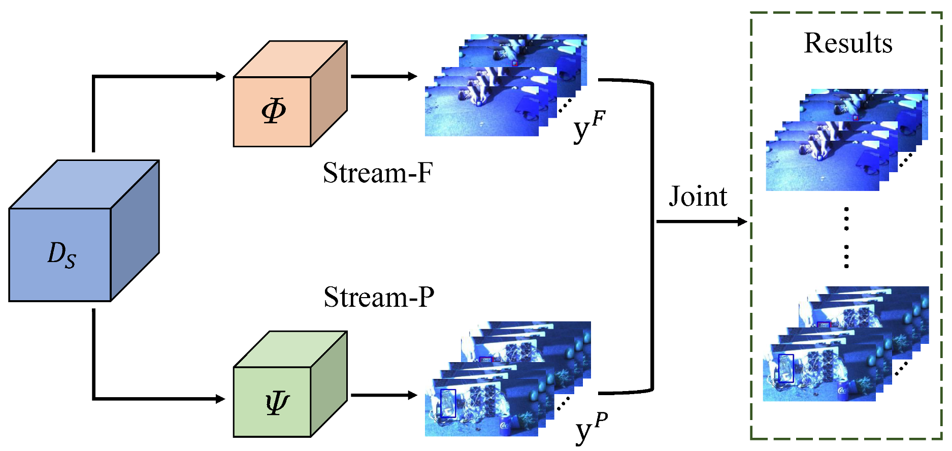
• For the first time, transfer learning technology was successfully applied in the field of HS object tracking. In particular, a new dual-transfer strategy is proposed—that is, the transfer learning method is adaptively selected according to the prior knowledge of the sample category, which not only solves the thorny problem of a lack of labeled data when learning deep models in the HS field but also verifies the applicability of transfer learning technology in the field of HS object tracking to a certain extent. This provides a flexible direction for future HS tracking research.
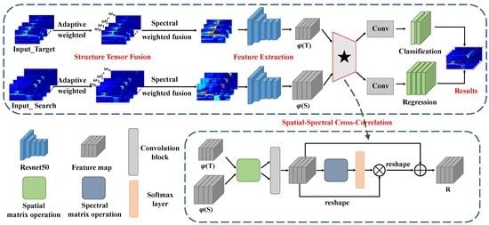
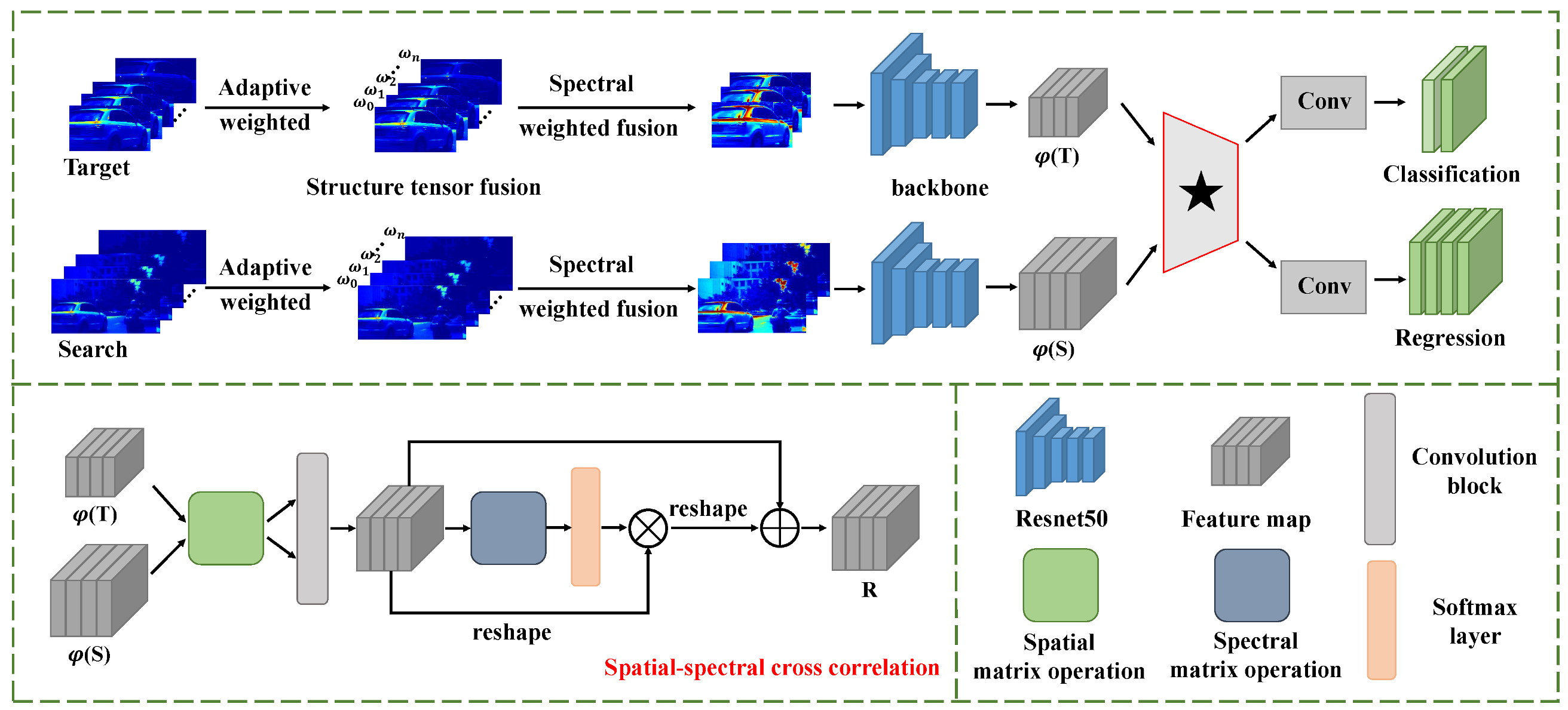
• For fully utilizing the spatial structure identification ability of the spatial dimension and the material identification ability of the spectral dimension in the HSIs, a novel spatial–spectral cross-correlation module is designed to better embed the spatial information and material information between the two branches of the Siamese network.
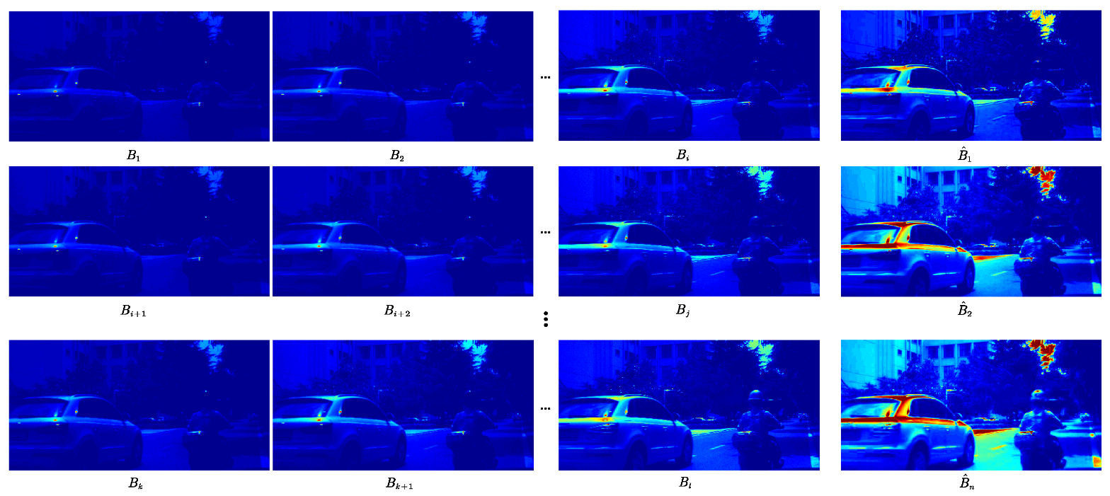
• Considering the high-dimensional characteristic of HS videos, we introduce an effective spectral weighted fusion method based on ST to gain the inputs of CNNs that consider the contribution rate to the significant information of each selected band to make our network more efficient.
• The experimental results demonstrate that, compared to the state of the art, the proposed SSDT-Net tracker offers more satisfactory performance based on a similar speed to the traditional color trackers. We provide an efficient and enlightening scheme for HS object tracking.

The rest of the paper is structured as follows. The basic theories related to transfer learning and trackers based on Siamese network structure are reviewed in Section 2. Section 3 details the proposed SSDT-Net. Section 4 displays our experimental results and comprehensive analyses of the method. Section 5 and Section 6 discuss and conclude our method, respectively.

2. Related Work

In this section, we briefly review two key aspects relevant to our work: hyperspectral video technology and the Siamese network-based trackers.

2.1. Hyperspectral Video Technology

Due to the limitations of sensors, traditional hyperspectral (HS) data are collected by sensors on satellites and are mostly used for remote sensing. However, recent advances in sensors have made it possible to collect HS sequences at close range at video rates. In paper [6], Xiong et al. published the first HS dataset captured by an HS camera in a close computer vision setting. They used a snapshot-spliced HS camera to collect the video. The HS camera can capture up to 180 HS images per second with each image having a spatial dimension of 512 × 256 pixels and a spectral dimension of 16 wavelengths ranging from 470 nm to 620 nm. During the collection of this dataset, the HS camera captures video at 25 frames per second (FPS).

To ensure high-quality hyperspectral images (HSIs), HS cameras also require pre-processing steps. This step includes spectral correction and image registration. Spectral correction mainly includes two steps: dark correction and spectral correction. The purpose of dark calibration is to eliminate the influence of noise generated by camera sensors by subtracting the dark frame from the captured image, where the dark frame is captured when the lens of an HS camera is covered by a lid. Spectral correction is designed to suppress the contribution of unnecessary second-order responses, such as the response to the wavelength leaking into the filter. The specific operation is to make the obtained spectrum more consistent with the expected spectrum by carrying out the sensor-specific spectral correction matrix for the obtained reflectivity.

At the same time, to more distinctly verify the advantages of material characteristics in target tracking and ensure a fair comparison with color-based tracking methods, Xiong et al. also obtained the RGB video corresponding to the HS video at the same frame rate from a close viewpoint and registered the HS sequence and color video so that they described almost the same scene. However, even then, there may be subtle differences between the two videos. Therefore, the authors of this dataset used the CIE color-matching function (CMFs) to convert HS videos into false color videos to ensure the complete consistency of data scenes. The CMFs represents the weight of each wavelength used to generate red, green, and blue channels in an HSI. Given an HSI $H\in {\mathbb{R}}^{W\times H\times B}$ with $W\times H$ pixels and B bands, we can convert the HSI to a CIE XYZ image using the following formula

$$I=\sum _{b=1}^{B}H\left(:,b\right)W\left(b,:\right)$$

(1)

where $W\in {\mathbb{R}}^{B\times 3}$ are the CMFs. The color transformation method in [20] is used to make the color intensity of the transformed image close to the corresponding RGB image collected.

Finally, in this paper, all experiments were performed based on this dataset, which contains videos of different modalities, namely HS, color, and false color. This enables our proposed HS tracker to be compared not only with other advanced HS trackers but also with other advanced color video trackers, which can more comprehensively demonstrate the advantages of our proposed algorithm.

2.2. Siamese Network-Based Trackers

The Siamese network is composed of two branches, which implicitly encode the original patches into another space and then fuse the two sets of information through a specific information embedding method. It is usually applied in contrastive tasks to compare the two branch features in the implicitly embedded space. Recently, the Siamese network has received extensive attention from the visual tracking community due to its well-balanced accuracy and speed [14,15,18].

Inspired by correlation-based approaches, recent mainstream trackers based on Siamese networks define visual tracking as a cross-correlation problem. They are anticipated to fully use the advantages of deep networks in end-to-end learning. SiamFC [14] first includes a fully connected convolution Siamese network to train the tracker and introduced the correlation layer as the fusion tensors, which greatly improved the fusion accuracy. Inspired by its success, many researchers have continued to study and propose novel models [17,21,22].

CFNet [17] introduces a correlation filter layer based on the SiamFC framework and conducts online tracking to improve the accuracy. DSiam [23] uses a dynamic Siamese network learning method through two online transformations of Siamese network branches, which obtains better tracking accuracy under the premise of balanced speed. SAsiam [21] constructs a double Siamese network consisting of semantic branches and appearance branches, which are trained separately for keeping the heterogeneity of features and integrated during testing for increasing the tracking accuracy.

To settle the problem of scale change, these Siamese networks adopt multi-scale search; however, this is time-consuming. To avoid the time-consuming steps in the stage of extracting multi-scale feature maps, the SiamRPN [16] tracker, inspired by the target detection region proposal network [24], utilizes the output of the Siamese network to extract region proposal through joint learning of the classification branch and regression branch. However, it is challenging to deal with disturbances that look similar to the object.

According to the structure of SiamRPN, DaSiamRPN [19] improves the resolution of the tracker through data enhancement, thus, obtaining more robust tracking results. Although these methods improve on the original SiamFC in many ways, the performance stall is mainly due to the weak backbone network (AlexNet) they use. SiamRPN++ [22] replaces AlexNet with ResNet [25]. During the training process, the position of the training object in the search area is moved randomly to eliminate the center deviation. This modification improves the tracking accuracy.

However, the performance evaluation of these existing Siamese network-based trackers is based on traditional color videos. To unleash the potential of the Siamese network for the processing of HS video, in this paper, we chose the Siamese network architecture as the backbone of our solution to solve the HS video tracking problem.

3. Proposed Method

We detail our proposed SSDT-Net for HS object tracking in this section. As shown in Figure 1 and Figure 2, our algorithm consists of five parts, dual-transfer strategy, spectral weighted fusion, feature extraction network, spatial–spectral cross-correlation module, and prediction head. The dual transfer strategy is a training method acting on the tracker. This strategy divides the target domain into two categories by measuring the similarity between the source domain and the target domain and adopts different training methods, while the inference method is unified.

The spectral weighted fusion is used as the data preprocessing module of the network. It calculates the significant information contribution rate of each band of HSI through ST and uses the contribution rate to perform adaptive weighted fusion on the original high-dimensional HSI data to make our network more efficient. The feature extraction network extracts the features of the search area and template and then uses the spatial–spectral cross-correlation module to obtain the similarity score matrix of the features. Finally, the prediction head performs binary classification and bounding box regression on the similarity matrix to generate the final tracking results. We present each component of SSDT-Net in detail in this section with some illustrations and discussions.

3.1. Dual Transfer

As is already known, traditional color videos contain millions of labeled natural images with thousands of categories. We use traditional color videos as the source domain for this transfer learning task. We first use our proposed spatial–spectral cross-correlation embedded network model to fully train on the source domain to obtain a knowledge weight, and then we fine-tune it on the HS dataset by freezing different numbers of network layers based on this knowledge weight. By analyzing the experimental results, we found that, for some categories, such as vehicles, animals, and people, the tracking accuracy increased as the number of frozen layers increased, while for other categories, such as paper, hard disk, circuit boards, and toys, as the number of frozen layers increased, the tracking accuracy became increasingly lower.

Then, we analyzed the reasons for this phenomenon in combination with the source domain and came to the conclusion that it is because the source domain we use is traditional RGB videos, and most of these datasets shoot scenes, such as vehicles, animals, and people. Therefore, in terms of the knowledge weight, we realize from the source domain training for these scenarios that the knowledge it learns is already very robust when used to test similar scenarios. On the contrary, if the feature extraction network is trained with very few such scenarios, it will lead to overfitting of the network, thereby, reducing the tracking accuracy. However, for scenarios where there is little or no presence in the source domain—that is, if the number of frozen layers is too many, a network on the dataset will not converge.

Based on the above analysis and inspired by [26], we propose a dual-transfer strategy that transfers traditional color video knowledge to the HS tracking task in different ways by measuring the similarity between the source domain and target domain. The specific operation is to use two different transfer learning methods according to the known prior information of each video category. As shown in Figure 1, the dual-transfer framework consists of two transfer learning streams.

Before formally introducing the strategy, we first introduce the notations used in this subsection. Let the source domain of transfer learning, i.e., traditional color videos, be represented by $D_S$, and the target domain of transfer learning, i.e., HS videos, be represented by $D_T$. The samples in the target domain that are similar to the source domain are defined as $D_{TF}$, and the samples in the target domain that are not similar to the source domain are defined as $D_{TP}$. The given test set of the target task is denoted as X. Similarly, the test set X can be divided into $X_F$ and $X_P$. Y represents the test results, consisting of $Y_F$ and $Y_P$. The following formula is established

$$\begin{array}{c}{D}_S=\{\{x_S^1,y_S^1\},\cdots ,\{x_S^M,y_S^M\}\}\hfill \\ D_T=\{\{x_T^1,y_T^1\},\cdots ,\{x_T^N,y_T^N\}\}\hfill \\ D_{TF}=\{\{x_T^1,y_T^1\},\cdots ,\{x_T^i,y_T^i\}\}\hfill \\ D_{TP}=\{\{x_T^{i+1},y_T^{i+1}\},\cdots ,\{x_T^N,y_T^N\}\}\hfill \\ X=\{\left\{x^1\right\},\cdots ,\left\{x^K\right\}\}\hfill \\ X_F=\{\left\{x^1\right\},\cdots ,\left\{x^j\right\}\}\hfill \\ X_P=\{\left\{x^{j+1}\right\},\cdots ,\left\{x^K\right\}\}\hfill \\ Y=\{\left\{y^1\right\},\cdots ,\left\{y^K\right\}\}\hfill \\ Y_F=\{\left\{y^1\right\},\cdots ,\left\{y^j\right\}\}\hfill \\ Y_P=\{\left\{y^{j+1}\right\},\cdots ,\left\{y^K\right\}\}\hfill \end{array}$$

(2)

where x is the data instance and y is the corresponding label or test results. The subscript represents the domain index and the superscript is the sample index. With these notations, the objective of HS tracking is to find a predict function f such that

$$Y=f\left(X,D_T,D_S\right)$$

(3)

For $D_{TF}$, we utilize the proposed spatial–spectral cross-correlation embedded network, which is first trained on $D_S$ and then used as knowledge to predict the outcome of the target task—that is, it is equivalent to transferring the knowledge of the source domain to obtain the features of the target domain. We call this a feature-based transfer learning method, which corresponds to stream-F in Figure 1. Denoting the classification and regression hypothesis as $\Phi \left(D_T,D_S\right)$ and considering Equation (3), the results of stream-F can be represented as

$$Y_F=f_F\left(X_F;\Phi \left(D_{TF},D_S\right)\right)$$

(4)

On the other hand, for $D_{TP}$, the knowledge parameters of the source domain are transferred to initialize our network, and $D_{TP}$ are trained based on knowledge weight parameters. We call this a parameter-based transfer learning method, which corresponds to stream-P in Figure 2. We denote the classification and regression in stream-P as $\Psi \left(D_T,D_S\right)$. Then, Equation (3) becomes

$$Y_P=f_P\left(X_P;\Psi \left(D_{TP},D_S\right)\right)$$

(5)

Combining Equations (4) and (5), the dual-transfer strategy is formulated as

$$Y=f_F\left(X_F;\Phi \left(D_{TF},D_S\right)\right)+f_P\left(X_P;\Psi \left(D_{TP},D_S\right)\right)$$

(6)

to integrate the two parts of the results together.

This method is different from some previous transfer learning methods. In this new scheme, we take full advantage of the prior knowledge of sample categories so that the existing knowledge is capable of solving different but related problems to a greater extent. We show that the transfer learning method is effective for the problem of object tracking in HS videos and that the proposed dual-transfer strategy is more effective than single transfer learning.

3.2. Spectral Weighted Fusion

To reduce the spectral dimensionality, we apply a spectral adaptive weighted fusion method. A band after spectral adaptive fusion is obtained by:

$${\widehat{B}}_n=\sum _{l=1}^L{\omega }_l{B}_l,n=1,2,\cdots ,N$$

(7)

where $B_l$ refers to the lth band and ${\left[{\omega }_1,{\omega }_2,\cdots {\omega }_L\right]}^T$ is the weight vector of each band. In particular, ST is exploited to obtain the weight vector adaptively, and the structure information of the image is represented with effect. According to Equation (7), the ST of the lth band at the ith pixel in an HSI can be expressed as:

$$S_i^l=\left[\begin{array}{cc}{\left(Y_i^l\right)}_x^2& {\left(Y_i^l\right)}_x{\left(Y_i^l\right)}_y\\ {\left(Y_i^l\right)}_x{\left(Y_i^l\right)}_y& {\left(Y_i^l\right)}_y^2\end{array}\right]$$

(8)

where $S_i^l$ is the ST of the lth band at the ith pixel. ${\left(Y_i^l\right)}_x=\left(\partial H^l/\partial x\right)$ and ${\left(Y_i^l\right)}_y=\left(\partial H^l/\partial y\right)$ stand for the gradient of the lth band at ith pixel along with the $x-$ and $y-$ directions. This ST $S_i^l$ can be decomposed as:

$$S_i^l=\left[\begin{array}{cc}{\eta }_{1,i}^l& {\eta }_{2,i}^l\end{array}\right]\left[\begin{array}{cc}{\lambda }_{1,i}^l& 0\\ 0& {\lambda }_{2,i}^l\end{array}\right]\left[\begin{array}{c}{\eta }_{1,i}^l\\ {\eta }_{2,i}^l\end{array}\right]$$

(9)

where ${\eta }_{1,i}^l$ and ${\eta }_{2,i}^l$ are the corresponding eigenvectors of the lth band at ith pixel and ${\lambda }_{1,i}^l,{\lambda }_{2,i}^l$ are the nonnegative eigenvalues of the lth band at the ith pixel. Assuming that ${\lambda }_{1,i}^l$ is the larger eigenvalue of the lth band at the ith pixel, i.e., ${\lambda }_{1,i}^l⩾{\lambda }_{2,i}^l$, then the larger eigenvalue, ${\lambda }_{1,i}^l$ indicates the edge strength of the lth band at the ith pixel, and the corresponding eigenvector, ${\eta }_{1,i}^l$, illustrates the direction in which the maximum gray value fluctuates.

If ${\lambda }_{1,i}^l>{\lambda }_{1,i}^{l+1}$, the edge strength of the lth band at the ith pixel is larger—that is, the lth band contains more structural information [27]. Therefore, its weight should be larger at the ith pixel. Similarly, the $\left(l+1\right)$th band should have a larger proportion of weight at the ith pixel in the case of ${\lambda }_{1,i}^l<{\lambda }_{1,i}^{l+1}$. When the eigenvalues of all bands are equal at the ith pixel, the weights of all bands are the same at this ith pixel, i.e., $1/l$.

Based on the analysis above, the weight vector for each band at the ith pixel can be gained by

$${\omega }_{d,i}=\frac{{\lambda }_{1,i}^l}{{\sum }_{d=1}^l{\lambda }_{1,i}^l},d=1,2,\cdots l$$

(10)

where ${\lambda }_{1,i}^l$ expresses the weight of the lth band at the ith pixel. In this way, the weight vector of each band can be obtained by Equation (10), and the appropriate bands can be adaptively weighted by Equation (7). Figure 3 shows the visualization results of the spectral weighted fusion of the l bands. It is clear that the fused bands can better represent the corners of the target. Finally, the sample band set consists of ${\widehat{B}}_1,{\widehat{B}}_2,\cdots ,{\widehat{B}}_n$. Considering the balance between computational cost and tracking performance, we set $n=3$.

3.3. Common Feature Extraction

Here, we make use of the CNN to structure the Siamese network structure to extract the common features. The Siamese network structure is comprised of two branches: one branch that learns the feature expression of the target T, and the other one that learns the feature presentation of the search area S. The two branches share the same CNN structure as their backbone networks, producing two feature maps $\phi \left(T\right)$ and $\phi \left(S\right)$. Low-level features, such as corners, shapes, edges, and colors, are indispensable visual attributes in location recognition, while high-level features are the key to semantic attribute recognition.

Therefore, many methods utilize the fusion of high-level and low-level features to better characterize the feature information of an image [22,28]. Here, we also consider the aggregate of multi-layer deep features to extract the common features. We utilize the modified ResNet-50 in [22] as our backbone model. To accomplish better recognition and inference discrimination, we associate the features extracted from the last three residual blocks of the backbone, which are expressed as ${\Gamma }_3\left(S\right),{\Gamma }_4\left(S\right)$, and ${\Gamma }_5\left(S\right)$. Specifically, the channel-wise concatenation is expressed as:

$$\phi \left(S\right)=Cat\left({\Gamma }_3\left(S\right),{\Gamma }_4\left(S\right),{\Gamma }_5\left(S\right)\right)$$

(11)

Then, to take full advantage of the abundant spatial–spectral information of two common feature maps, $\phi \left(T\right)$ and $\phi \left(S\right)$, we propose a spatial–spectral cross-correlation module to embed the information of these two branches as discussed in the next subsection.

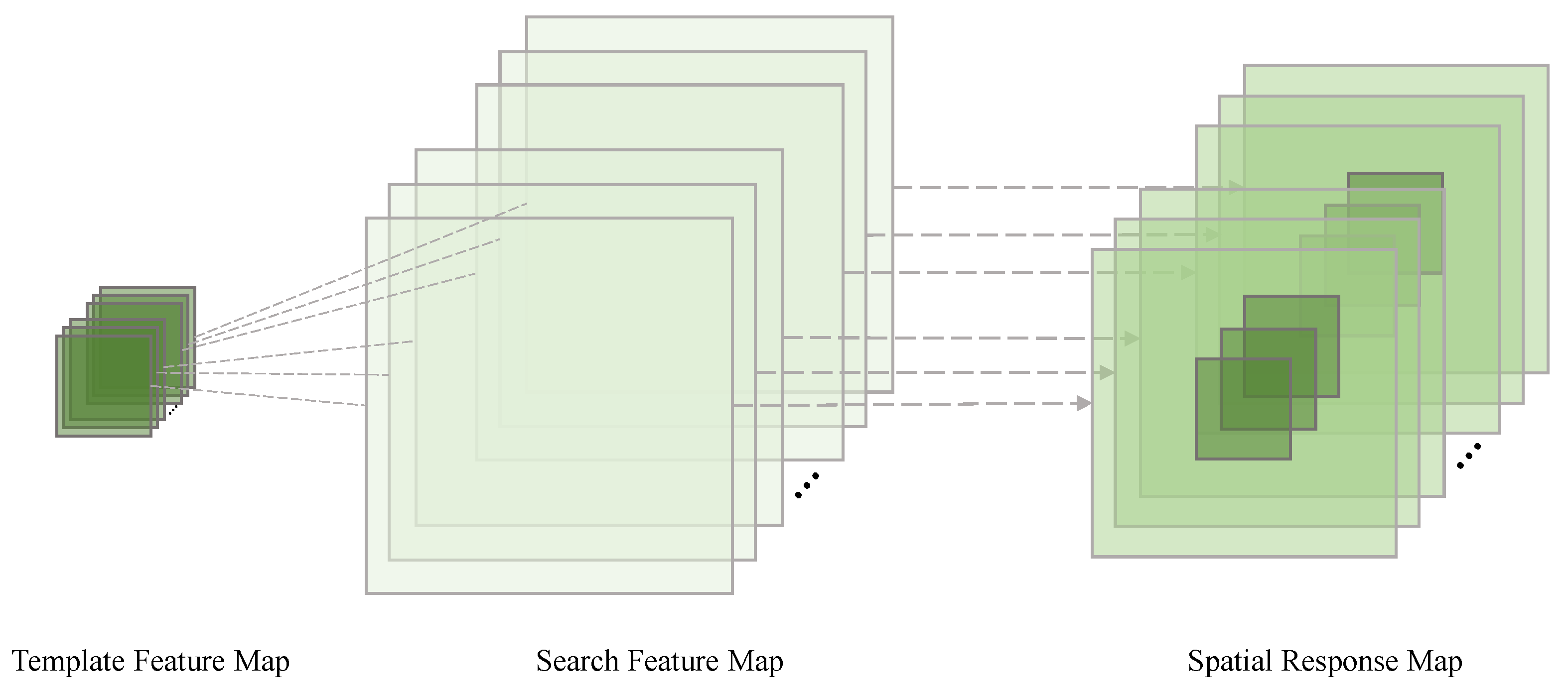
3.4. Spatial–Spectral Cross-Correlation

The cross-correlation module is the essential operation of embedding the information of two branches. As we know, in some deep learning trackers for traditional color videos, such as SiamFC, SiamRPN, and SiamRPN++, some cross-correlation modules are proposed. SiamFC gains a single-channel response map for object localization by taking advantage of a cross-correlation layer. SiamRPN scales the channels by adding a large convolution layer so that the cross-correlation module can embed higher levels of information (UP-XCorr). In SiamRPN++, the depth-wise cross-correlation (DW-XCorr) is proposed, which performs the cross-correlation operation channel by channel to achieve efficient information association.

Figure 2 shows a spatial–spectral cross-correlation (SS-XCorr) module. The module first performs spatial matrix operations on the output features $\phi \left(T\right)$ and $\phi \left(S\right)$ of the feature extraction network. Then, we subject them to a grouped convolution operation to spatially correlate each channel to generate a response map $R_1^{W\times H\times B}$. The response map $R_1^{W\times H\times B}$ has the same number of channels as the common feature maps $\phi \left(T\right)$ and $\phi \left(S\right)$. The specific operation process is shown in Figure 4.

Here, we use the template feature map as the convolution kernel of the convolution, the search feature map as the input of the convolution, and use grouped convolution to perform channel-by-channel spatial cross-correlation operations on the template and search feature maps to obtain the spatial response map. For HS data, the channel dimension can be equivalent to the spectral dimension. Taking advantage of the hyperspectral correlation between adjacent bands, we can highlight the channels with more important information in the spatial response map. Therefore, we perform spectral matrix operations on the response map $R_1^{W\times H\times B}$, and we use a softmax layer to gain the spectral attention map $X^{B\times B}$.

Moreover, we perform a matrix multiplication between the transformation of $R_1^{W\times H\times B}$ and $X^{B\times B}$ and reshape their result to $R_1^{{}^{\prime }W\times H\times B}$. Then, we perform an element-wise sum operation between $R_1$ and $R_1^{\prime }$ to gain the final response map $R^{W\times H\times B}$. The generated response map R models the long-range semantic correlation between spectral–spatial feature maps, and it includes massive information for classification and regression.

Figure 5a,b are the visualization results of the similarity matrix using the DW-XCorr module and the SS-XCorr module, respectively. It is evident that our proposed SS-XCorr module enhances the discrimination of distractors in the target tracking task.

3.5. Bounding Box Prediction

Every position in the response map R can be mapped back to the input search area S. The bounding box prediction task is divided into two subtasks: one is the classification of target and background, and the other is the regression branch for the positioning of the target bounding box. For the response map $R^{W\times H\times L}$, the classification branch outputs a feature map $D_{W\times H\times 2}^{cls}$ for classification, and the regression branch produces a regression feature map $D_{W\times H\times 4}^{reg}$. As shown in Figure 2, each point in $D_{W\times H\times 2}^{cls}$ involves a $2D$ vector, which represents positive and negative scores of each anchor at the corresponding position on the input search region. Similarly, each point in $D_{W\times H\times 4}^{reg}$ involves a $4D$ vector, which expresses the distances between the anchor and the relevant ground truth.

Inspired by [24], we also utilize the cross-entropy loss for classification and the smooth $L_1$ loss with normalized coordinates for regression. Let $A_x,A_y,A_w$, and $A_h$ represent the center point and shape of the anchor boxes, respectively, and $G_x,G_y,G_w$, and $G_h$ represent those of the ground truth boxes, respectively. The normalized distance is:

$$\begin{array}{c}{d}_x=\left(G_x-A_x\right)/A_w,d_y=\left(G_y-A_y\right)/A_h\hfill \\ d_w=ln\left(G_w/A_w\right),d_h=ln\left(G_h/A_h\right)\hfill \end{array}$$

(12)

The regression loss is:

$$L_{reg}=\sum _{i\in \left\{x,y,w,h\right\}}smoot{h}_{L_1}\left(d_i,\sigma \right)$$

(13)

where

$$smoot{h}_{L_1}\left(x,\sigma \right)=\left\{\begin{array}{cc}0.5{\sigma }^2{x}^2,\hfill & \left|x\right|<\frac{1}{{\sigma }^2}\hfill \\ \left|x\right|-\frac{1}{2{\sigma }^2},\hfill & \left|x\right|⩾\frac{1}{{\sigma }^2}\hfill \end{array}\right.$$

(14)

is a smooth $L_1$ loss.

The overall loss function is

$$Loss=L_{cls}+\lambda L_{reg}$$

(15)

where $L_{cls}$ is the cross-entropy loss for classification, and the weighting parameter $\lambda$ is empirically set to be 1.2 for stable tracking performance.

4. Experiments

In this section, we describe our experimental setup, compare the performance of our proposed SSDT-Net tracker against several typical color trackers and HS trackers, and present an ablation study to emphasize the importance of different components of our model.

4.1. Experimental Setup

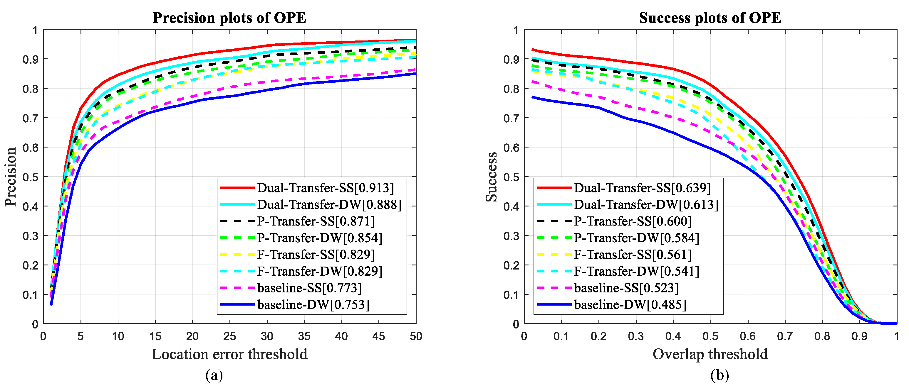
Data Description: The color video data sets commonly used by traditional color video trackers act as the source domain for transfer learning, including COCO [29], YouTube-BoundingBoxes Dataset [30], ImageNet VID, and ImageNet DET [31]. COCO contains 80 categories and 200,000 images, the ImageNet DET and ImageNet VID datasets contain 200 object categories, and the YouTube-BoundingBoxes Dataset contains 10.5 million manually labeled frames on 23 object categories. The dataset provided by the HS object tracking competition is used as the object domain and target task for transfer learning.

The dataset is acquired by a XIMEA SNm4x4 VIS Camera and consisted of 40 training videos and 35 testing videos, each containing HS, RGB videos, and false-color in the same scene. The HS datasets were shot at 25 frames per second (FPS). Each frame was initially captured from a 2D image with 16 bands arranged in a mosaic pattern. Each frame was then converted to 3D, with the first two dimensions representing the position of each pixel and the third dimension representing the band number. The 16 bands cover the range from 470 to 620 nm, and each band is 512 × 256 pixels in size. RGB video was also obtained at the same frame rate at viewpoints very close to the HS video. The dataset also provides false-color videos converted from HS videos.

Evaluation Metrics: We employ the four most commonly used object tracking evaluation indexes, including success plot, precision plot, area under the curve (AUC), and the average distance precision scores at a threshold of 20 pixels (DP@20P), to compare the performance of the proposed method with its comparison methods quantitatively. However, it should be noted that most of the representative object tracking algorithm codes based on HS videos have not yet become open source, and thus we only use AUC as the evaluation index for quantitative comparison.

The success plot indicates the percentages of successful frames whose predicted bounding box and ground-truth overlap ratio is greater than a certain threshold within 0 and 1. A precision plot records the percentage of video frames whose distance between the center point of the estimated object position and the center point of the ground truth is less than a given threshold. Different thresholds result in different percentages; therefore, a curve can be obtained. All the results are presented through a one-pass evaluation (OPE), where the tracker runs through the entire test sequence and is initialized from the ground truth position in the initial frame.

Implementation Details: Our proposed approach was implemented in Python with PyTorch and trained on four RTX 2080Ti cards. The backbone network was pre-trained on ImageNet for image labeling, which has a good initialization effect on other tasks [32,33]. In stream-F, we train our network on the source domain and then use it as a knowledge model to predict the outcome of the object task. In stream-P, we initialize our network with the knowledge model of the source domain and then train it on the target domain to estimate the knowledge weight, which is utilized to predict the result of the target task. During this process, we set the batch size to 128, utilize Stochastic Gradient Descent (SGD) with an initial learning rate of 0.005, and perform a total of 20 epochs.

For the first five epochs, the parameters of the Siamese network are frozen while training the regression and classification branches. For the last 15 epochs, the entire network is trained end-to-end with an exponential drop in learning rate from 0.01 to 0.0005.

4.2. Ablation Study

An ablation study was conducted to demonstrate the validity of the proposed components by evaluating several variants of the SSDT-Net tracker on HS videos. We utilize the results of the network training from scratch as the baseline.

Dual Transfer:Figure 6 shows the success plots and precision plots of the baseline, feature-based transfer learning, parameter-based transfer learning, and dual-transfer learning strategy. The three transfer learning methods achieved significant improvement compared with the baseline. Here, feature-based transfer represents the result of overfitting of similar scenes in the source and target domains, while parameter-based transfer represents the result of network divergence in different scenes. As shown in

Table 1. Ablation study of our proposed tracker on HS videos.

Transfer Strategy	Corr	AUC	DP@20P
Baseline	DW	0.4848	0.7533
	SS	0.5233	0.7727
Feature-based Transfer	DW	0.5414	0.8289
	SS	0.5608	0.8289
Parameter-based Transfer	DW	0.5839	0.8540
	SS	0.6001	0.8710
Dual-transfer	DW	0.6126	0.8875
	SS	0.6391	0.9132

DW and SS represent depth-wise cross-correlation and spatial–spectral cross-correlation, respectively. Red marks the top value.

, the value of AUC obtained reached $0.4848$ and $0.5233$ for the baseline when utilizing the DW-XCorr module and SS-XCorr module to embed information. When employing feature-based transfer learning, the performance of each group was significantly improved by $5.66\%$ and $3.75\%$, respectively.

Similarly, when employing parameter-based transfer learning, the method yielded better results with tracking improved by $9.91\%$ and $7.68\%$. With the dual-transfer learning strategy, the performance improved further by $12.78\%$ and $11.58\%$. The numerical results indicate that the transfer learning method is effective for the problem of object tracking in HS videos, and this also confirms the correctness of our theoretical reasoning. Feature-based transfer learning may lead to the overfitting of similar scenes in the source and target domains, and parameter-based transfer learning may cause the divergence of networks in different scenes. The proposed dual-transfer strategy is more effective than single-transfer learning.

Spatial–Spectral Cross-Correlation (SS-XCorr): Figure 6 and Table 1 report the results of the network using DW-XCorr and SS-XCorr. Intuitively, it is expected that the SS-XCorr can be helpful because, for HS data, it is crucial to make good use of spatial–spectral joint information for the processing of its related tasks. This is indeed apparent in Table 1 where an increase in AUC is clear in the four states of the network with SS-XCorr. The value of the AUC obtained reached $0.4848$, $0.5414$, $0.5839$, and $0.6126$ for the baseline and three transfer learning strategies when utilizing the DW-XCorr module to embed information, respectively.

When utilizing the SS-XCorr module to embed information, the method yielded better results, with tracking results up to $3.85\%$, $1.94\%$, $1.62\%$, and $2.65\%$, respectively. Therefore, combining the spatial structure identification ability of the spatial dimension and the material identification ability of the spectral dimension in the HSIs is effective for more accurate object tracking.

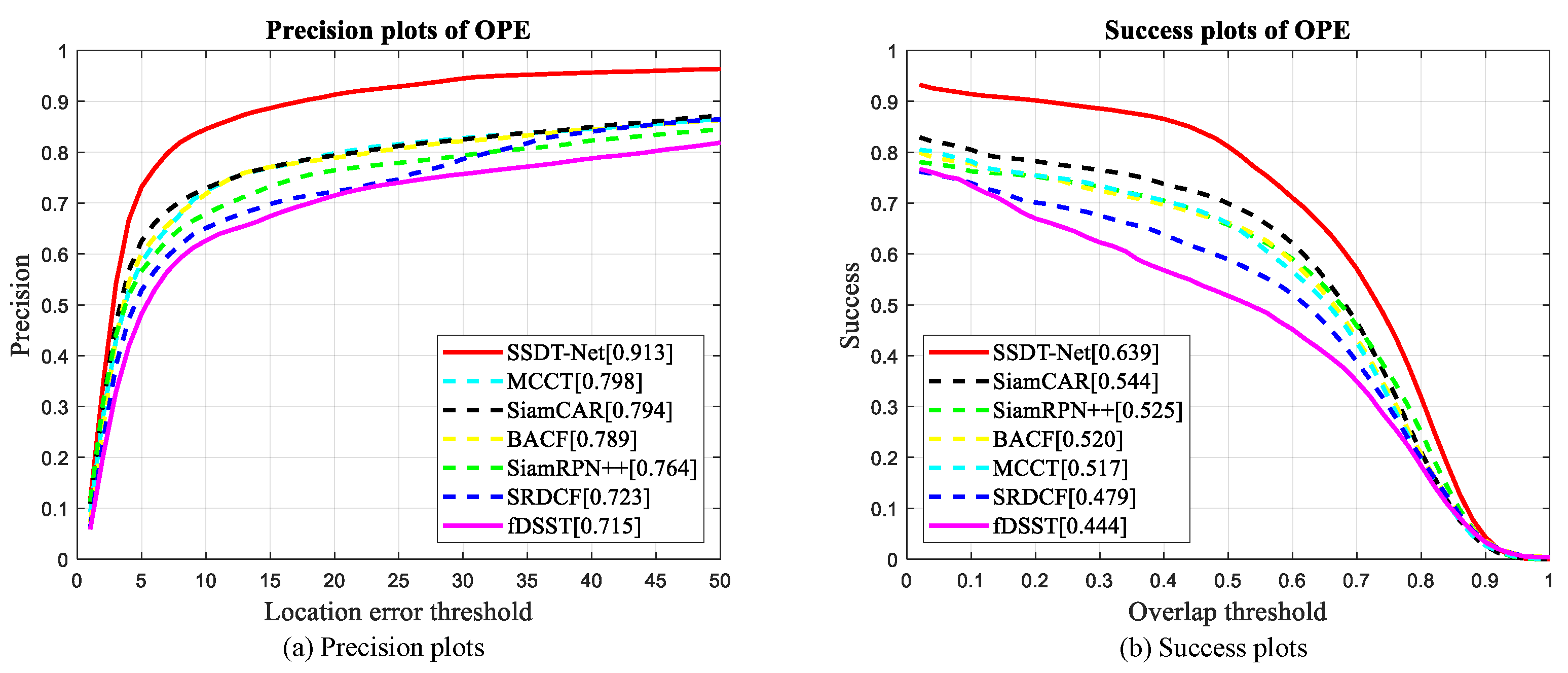
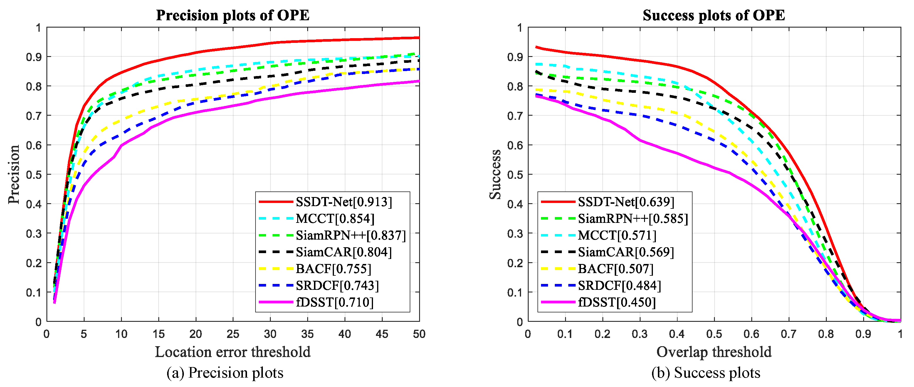
4.3. Quantitative Comparison with the State-Of-The-Art Color Trackers

The proposed SSDT-Net tracker was compared with six state-of-the-art color trackers, including the BACF [34], fDSST [35], MCCT [36], SRDCF [37], SiamRPN++, and SiamCAR [38] methods. fDSST is a scale-adaptive tracking method that learns two distinguishing correlation filters for scale estimation and object localization. SRDCF and BACF aim to regularize the correlation filter on the basis of the spatial distribution to reduce the boundary effect on training samples prompted by periodic assumptions. MCCT brings together numerous experts to track objects through diverse levels of features.

SiamRPN++ is a modified method based on SiamRPN, which uses a deeper Siamese network to attach a sub-network for region proposal (RPN) extraction and performs visual tracking through joint training of a regression branch and a classification branch. By splitting the visual tracking problem into two sub-problems of pixel object bounding box regression and pixel classification, SiamCAR deploys a new fully convolutional Siamese network to settle the end-to-end visual tracking problem in a pixel-by-pixel manner.

The SSDT-Net tracker is tested on HS data. Since the contrast trackers selected were exploited for RGB data, they all run on both RGB data and false-color data converted from HS data. Figure 7 and Figure 8 show the success plots and precision plots of the SSDT-Net tracker on HS videos and all color trackers on false-color videos generated from HS videos and RGB videos, respectively. The results indicate that the performance of the deep feature-based trackers in color video trackers is better than most of the handcrafted feature-based trackers. For trackers based on hand-crafted features, MCCT brings together multiple experts to track objects through different levels of features, resulting in better tracking performance.

In addition, as shown in

Table 2. Performance comparison with color video trackers in terms of the AUC and DP@20P.

Tracker	HS/False-Color Videos		Color Videos
	AUC	DP@20P	AUC	DP@20P
BACF	0.5198	0.7889	0.5072	0.7549
fDSST	0.4442	0.7149	0.4499	0.7099
MCCT	0.5170	0.7984	0.5709	0.8542
SRDCF	0.4793	0.7229	0.4837	0.7433
SiamRPN++	0.5253	0.7643	0.5852	0.8371
SiamCAR	0.5441	0.7936	0.5688	0.8044
SSDT-Net	0.6391	0.9132	-	-

The top two values are marked by red and blue.

compared with the above color video trackers, the SSDT-Net tracker we proposed ranked the highest over a range of thresholds by achieving an AUC of $0.6391$ and a DP@20P of $0.9132$. When using traditional color videos, the highest performance color video tracker was SiamRPN, with the values of AUC and DP@20P reaching $0.5852$ and $0.8371$, respectively. In comparison, the AUC and DP@20P of the SSDT-Net tracker improved by $5.39\%$ and $7.61\%$.

Analogously, when employing false-color videos, SiamCAR achieved the highest performance, with the values of AUC and DP@20 reaching $0.5441$ and $0.7936$. In comparison, the SSDT-Net tracker yielded better results, with tracking improving by $9.50\%$ and $11.96\%$. Numerical results confirm that the SSDT-Net tracker can make good use of the knowledge transferred from the color videos as well as local spatial information and the detailed constituent material distribution information of the HS data to represent the image content, which helps the tracker to distinguish the object from the background.

4.4. Quantitative Comparison with the State-Of-The-Art Hyperspectral Trackers

The SSDT-Net tracker was compared with three recent HS trackers, SST-Net, BAE-Net, and MHT. MHT is a tracker based on handcrafted features that embed the spectral–spatial information of the HS image into a multi-dimensional gradient histogram and combines it with the global material abundance feature to describe the target. Both BAE-Net and SST-Net take advantage of deep features. BAE-Net converts HSI based on spectral information into massive false-color images. These converted images generate several weak trackers through several VITAL trackers for subsequent ensemble learning to acquire the object positions. SST-Net combines spatial, spectral, and temporal attention based on BAE-Net to better select valuable HS bands for deep ensemble tracking.

Table 3. Performance comparison with hyperspectral trackers of AUC.

Video	SSDT-Net	MHT	BAE-Net	SST-Net
Hyperspectral	0.6391	0.6080	0.6060	0.6230

The top two values are marked by red and blue.

demonstrates the comparative results of these HS trackers. Although the BAE-Net tracker is based on data-driven deep features, the MHT tracker based on handcrafted features achieves higher tracking accuracy compared to the BAE-Net tracker because of its limited annotation data used for training and only utilizing the spectral information of HS data.

Moreover, on the basis of BAE-Net, SST-Net increases the use of spatial-temporal information when converting HSI, which can describe the object more effectively and produce better tracking performance. For the SSDT-Net tracker, the prior knowledge of a large number of color tracking videos is fully utilized, and spectral–spatial information is considered simultaneously to extract object features, yielding the highest tracking accuracy, with an AUC value of $0.6391$. The AUC value was further improved by $1.61\%$, compared with SST-Net, which is second only to the SSDT-Net tracker.

4.5. Running Time Comparison

Table 4. Running time comparison (FPS).

Videos	SSDT-Net	MHT	BACF	fDSST
RGB	-	-	60.6	120.6
Hyperspectral/False-Color	35.7	6.09	66.36	120.1
Videos	MCCT	SRDCF	SiamRPN++	SiamCAR
RGB	7.5	24.3	35.2	52.3
Hyperspectral/False-Color	7.3	25.8	35.5	52.5

reports the tracking speed of six state-of-the-art color trackers and two state-of-the-art HS trackers on CPUs and GPUs concerning frames per second (FPS), respectively. BACF, fDSST, MCCT, SRDCF, and MHT were implemented on Windows machines equipped with Intel(R) Core(TM) i5-10500 CPU @ 3.10GHz and 32GB of RAM. SSDT-Net, SiamRPN++, and SiamCAR are performed in Python with PyTorch and trained on four RTX 2080Ti cards. fDSST attained the best speed on both videos on CPUs. SSDT-Net achieved similar speed with deep color trackers. The experimental results prove that our HS tracker can acquire better tracking performance based on a similar speed with state-of-the-art traditional color trackers.

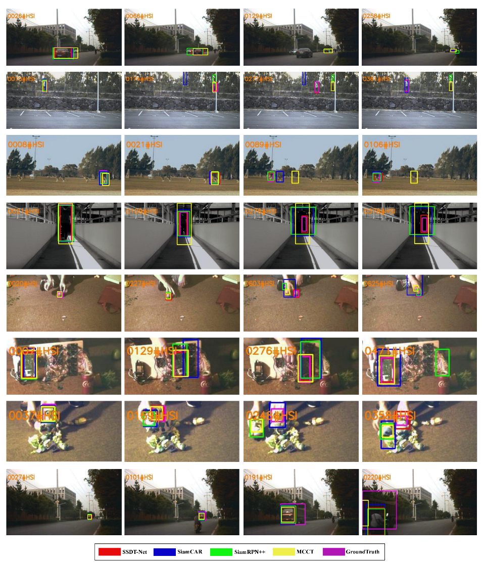
4.6. Demonstrations of Visual Tracking Results

Figure 9 visually compares the tracking results of the SSDT-Net tracker with several color trackers on sample HS or false-color videos. It can be seen that the SSDT-Net tracker also provides the best visualization results in complex scenes, such as background clutter, target appearance similar to background, and target appearance changing rapidly. The results demonstrate the high robustness of the spatial structure identification ability and material identification ability brought by the rich spatial–spectral information of HS data, as well as the effectiveness of transfer learning applied to HS object tracking.

5. Discussion

Although the effectiveness of the proposed SSDT-Net was verified by comprehensive and convincing experiments and analysis, there are still some interesting details that are further discussed below as future work:

1.

As shown in Section 3.2, we directly use the spectral weighted fusion module based on the ST to fuse the data at the input end of the network to reduce the dimension and perform the fusion operation at the input of the network; although the tracker can obtain excellent speed, it will cause a great deal of loss of information, and the material identification characteristics of HS data will limit the performance improvement of the tracker. Therefore, in the following research, we can consider the fusion of feature maps after feature extraction on the network so as to make better use of the spectral information of HS data.

2.

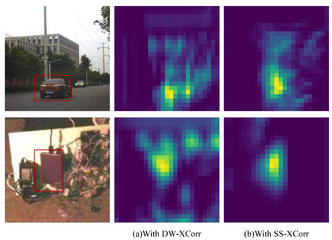
The experimental results show that the spectral cross-correlation module plays a role, improves the subjective and objective effects, and proves the effectiveness of spectral information for target recognition. Therefore, we can consider further investigation of spectral cross-correlation operations.

3.

Regarding the cross-correlation module of the Siamese network, the correlation operation itself is a local linear matching process, and it is easy to lose semantic information and fall into a local optimum, which may become a bottleneck in designing high-precision tracking algorithms. Therefore, inspired by Transformer, we consider using the attention mechanism to perform cross-correlation operation, which requires further study.

6. Conclusions

In this paper, we proposed a novel HS tracker based on transfer learning, i.e., SSDT-Net, for the first time in the field of HS object tracking. The key points of this method are to transfer the knowledge of traditional color videos to the HS tracking task through transfer learning and to distinguish the target and background by combining the spatial structure information and material information of the HS data. Therefore, the superiority of the SSDT-Net tracker is due to several aspects.

First, the proposed dual-transfer strategy based on transfer learning makes the best use of color video information to solve the HS video tracking problem. Then, we take advantage of our proposed spatial–spectral cross-correlation module to better embed spatial and material information between the two branches of the Siamese network.

Furthermore, to make our network more efficient under the premise of ensuring high performance, a novel spectral weighted fusion method based on ST was adopted to gain the inputs of the network. Experiments performed on HS videos demonstrated that the proposed SSDT-Net tracker exhibited excellent performance in terms of quantitative evaluation and visual comparison based on its similar speed to state-of-the-art traditional color trackers.

References

1. Marvasti-Zadeh, S.M.; Cheng, L.; Ghanei-Yakhdan, H.; Kasaei, S. Deep Learning for Visual Tracking: A Comprehensive Survey. IEEE Trans. Intell. Transp. Syst. 2021, 23, 1–26. [Google Scholar] [CrossRef]
2. Gao, J.; Zhang, T.; Yang, X.; Xu, C. Deep Relative Tracking. IEEE Trans. Image Process. 2017, 26, 1845–1858. [Google Scholar] [CrossRef]
3. Liang, J.; Zhou, J.; Tong, L.; Bai, X.; Wang, B. Material based salient object detection from hyperspectral images. Pattern Recognit. 2018, 76, 476–490. [Google Scholar] [CrossRef] [Green Version]
4. Okwuashi, O.; Ndehedehe, C.E. Deep support vector machine for hyperspectral image classification. Pattern Recognit. 2020, 103, 107298. [Google Scholar] [CrossRef]
5. Qian, K.; Zhou, J.; Xiong, F.; Zhou, H.; Du, J. Object tracking in hyperspectral videos with convolutional features and kernelized correlation filter. In International Conference on Smart Multimedia; Springer: Berlin/Heidelberg, Germany, 2018; pp. 308–319. [Google Scholar]
6. Xiong, F.; Zhou, J.; Qian, Y. Material based object tracking in hyperspectral videos. IEEE Trans. Image Process. 2020, 29, 3719–3733. [Google Scholar] [CrossRef] [PubMed]
7. Uzkent, B.; Rangnekar, A.; Hoffman, M.J. Tracking in aerial hyperspectral videos using deep kernelized correlation filters. IEEE Trans. Geosci. Remote Sens. 2018, 57, 449–461. [Google Scholar] [CrossRef] [Green Version]
8. Simonyan, K.; Zisserman, A. Very Deep Convolutional Networks for Large-Scale Image Recognition. In Proceedings of the 3rd International Conference on Learning Representations, ICLR 2015, San Diego, CA, USA, 7–9 May 2015. [Google Scholar]
9. Li, Z.; Xiong, F.; Zhou, J.; Wang, J.; Lu, J.; Qian, Y. BAE-Net: A Band Attention Aware Ensemble Network for Hyperspectral Object Tracking. In Proceedings of the 2020 IEEE International Conference on Image Processing (ICIP), Abu Dhabi, United Arab Emirates, 25–28 October 2020; pp. 2106–2110. [Google Scholar]
10. Song, Y.; Ma, C.; Wu, X.; Gong, L.; Bao, L.; Zuo, W.; Shen, C.; Lau, R.W.; Yang, M.H. Vital: Visual tracking via adversarial learning. In Proceedings of the 2018 IEEE/CVF Conference on Computer Vision and Pattern Recognition, Salt Lake City, UT, USA, 18–23 June 2018; pp. 8990–8999. [Google Scholar]
11. Li, Z.; Ye, X.; Xiong, F.; Lu, J.; Zhou, J.; Qian, Y. Spectral-Spatial-Temporal Attention Network for Hyperspectral Tracking. Available online: http://www.ieee-whispers.com/wp-content/uploads/2021/03/WHISPERS_2021_paper_55.pdf (accessed on 26 March 2021).
12. Liu, Z.; Wang, X.; Shu, M.; Li, G.; Sun, C.; Liu, Z.; Zhong, Y. An Anchor-Free Siamese Target Tracking Network for Hyperspectral Video. Available online: http://www.ieee-whispers.com/wp-content/uploads/2021/03/WHISPERS_2021_paper_52.pdf (accessed on 26 March 2021).
13. Pan, S.J.; Yang, Q. A survey on transfer learning. IEEE Trans. Geosci. Remote Sens. 2009, 22, 1345–1359. [Google Scholar] [CrossRef]
14. Bertinetto, L.; Valmadre, J.; Henriques, J.F.; Vedaldi, A.; Torr, P.H. Fully-convolutional siamese networks for object tracking. In European Conference on Computer Vision; Springer: Berlin/Heidelberg, Germany, 2016; pp. 850–865. [Google Scholar]
15. Held, D.; Thrun, S.; Savarese, S. Learning to track at 100 fps with deep regression networks. In European Conference on Computer Vision; Springer: Berlin/Heidelberg, Germany, 2016; pp. 749–765. [Google Scholar]
16. Li, B.; Yan, J.; Wu, W.; Zhu, Z.; Hu, X. High performance visual tracking with siamese region proposal network. In Proceedings of the 2018 IEEE/CVF Conference on Computer Vision and Pattern Recognition, Salt Lake City, UT, USA, 18–23 June 2018; pp. 8971–8980. [Google Scholar]
17. Valmadre, J.; Bertinetto, L.; Henriques, J.; Vedaldi, A.; Torr, P.H. End-to-end representation learning for correlation filter based tracking. In Proceedings of the 2017 IEEE Conference on Computer Vision and Pattern Recognition (CVPR), Honolulu, HI, USA, 21–26 July 2017; pp. 2805–2813. [Google Scholar]
18. Wang, Q.; Gao, J.; Xing, J.; Zhang, M.; Hu, W. Dcfnet: Discriminant correlation filters network for visual tracking. arXiv 2017, arXiv:1704.04057. [Google Scholar]
19. Zhu, Z.; Wang, Q.; Li, B.; Wu, W.; Yan, J.; Hu, W. Distractor-aware siamese networks for visual object tracking. In European Conference on Computer Vision; Springer: Berlin/Heidelberg, Germany, 2018; pp. 101–117. [Google Scholar]
20. Pitie, F.; Kokaram, A. The linear monge-kantorovitch linear colour mapping for example-based colour transfer. In Proceedings of the 4th European Conference on Visual Media Production, London, UK, 27–28 November 2007; pp. 1–9. [Google Scholar]
21. He, A.; Luo, C.; Tian, X.; Zeng, W. A twofold siamese network for real-time object tracking. In Proceedings of the 2018 IEEE/CVF Conference on Computer Vision and Pattern Recognition, Salt Lake City, UT, USA, 18–23 June 2018; pp. 4834–4843. [Google Scholar]
22. Li, B.; Wu, W.; Wang, Q.; Zhang, F.; Xing, J.; Yan, J. Siamrpn++: Evolution of siamese visual tracking with very deep networks. In Proceedings of the 2019 IEEE/CVF Conference on Computer Vision and Pattern Recognition (CVPR), Long Beach, CA, USA, 15–20 June 2019; pp. 4282–4291. [Google Scholar]
23. Guo, Q.; Feng, W.; Zhou, C.; Huang, R.; Wan, L.; Wang, S. Learning dynamic siamese network for visual object tracking. In Proceedings of the 2017 IEEE International Conference on Computer Vision (ICCV), Venice, Italy, 22–29 October 2017; pp. 1763–1771. [Google Scholar]
24. Ren, S.; He, K.; Girshick, R.; Sun, J. Faster R-CNN: Towards Real-Time Object Detection with Region Proposal Networks. IEEE Trans. Pattern Anal. Mach. Intell. 2017, 39, 1137–1149. [Google Scholar] [CrossRef] [PubMed] [Green Version]
25. He, K.; Zhang, X.; Ren, S.; Sun, J. Deep residual learning for image recognition. In Proceedings of the 2016 IEEE Conference on Computer Vision and Pattern Recognition (CVPR), Las Vegas, NV, USA, 27–30 June 2016; pp. 770–778. [Google Scholar]
26. Han, Y.; Huang, G.; Song, S.; Yang, L.; Wang, H.; Wang, Y. Dynamic neural networks: A survey. IEEE Trans. Pattern Anal. Mach. Intell. 2021. [Google Scholar] [CrossRef] [PubMed]
27. Xie, W.; Jiang, T.; Li, Y.; Jia, X.; Lei, J. Structure tensor and guided filtering-based algorithm for hyperspectral anomaly detection. IEEE Trans. Geosci. Remote Sens. 2019, 57, 4218–4230. [Google Scholar] [CrossRef]
28. Ma, C.; Huang, J.B.; Yang, X.; Yang, M.H. Robust Visual Tracking via Hierarchical Convolutional Features. IEEE Trans. Pattern Anal. Mach. Intell. 2017, 25, 670–674. [Google Scholar] [CrossRef] [PubMed] [Green Version]
29. Lin, T.Y.; Maire, M.; Belongie, S.; Hays, J.; Perona, P.; Ramanan, D.; Dollár, P.; Zitnick, C.L. Microsoft coco: Common objects in context. In European Conference on Computer Vision; Springer: Berlin/Heidelberg, Germany, 2014; pp. 740–755. [Google Scholar]
30. Real, E.; Shlens, J.; Mazzocchi, S.; Pan, X.; Vanhoucke, V. Youtube-boundingboxes: A large high-precision human-annotated data set for object detection in video. In Proceedings of the 2017 IEEE Conference on Computer Vision and Pattern Recognition (CVPR), Honolulu, HI, USA, 21–26 July 2017; pp. 5296–5305. [Google Scholar]
31. Russakovsky, O.; Deng, J.; Su, H.; Krause, J.; Satheesh, S.; Ma, S.; Huang, Z.; Karpathy, A.; Khosla, A.; Bernstein, M.; et al. Imagenet large scale visual recognition challenge. Int. J. Comput. Vis. 2015, 115, 211–252. [Google Scholar] [CrossRef] [Green Version]
32. He, K.; Gkioxari, G.; Dollár, P.; Girshick, R. Mask r-cnn. In Proceedings of the 2017 IEEE International Conference on Computer Vision (ICCV), Venice, Italy, 22–29 October 2017; pp. 2961–2969. [Google Scholar]
33. Long, J.; Shelhamer, E.; Darrell, T. Fully convolutional networks for semantic segmentation. In Proceedings of the 2015 IEEE Conference on Computer Vision and Pattern Recognition (CVPR), Boston, MA, USA, 7–12 June 2015; pp. 3431–3440. [Google Scholar]
34. Kiani Galoogahi, H.; Fagg, A.; Lucey, S. Learning background-aware correlation filters for visual tracking. In Proceedings of the 2017 IEEE International Conference on Computer Vision (ICCV), Venice, Italy, 22–29 October 2017; pp. 1135–1143. [Google Scholar]
35. Danelljan, M.; Häger, G.; Khan, F.S.; Felsberg, M. Discriminative scale space tracking. IEEE Trans. Pattern Anal. Mach. Intell. 2016, 39, 1561–1575. [Google Scholar] [CrossRef] [PubMed] [Green Version]
36. Wang, N.; Zhou, W.; Tian, Q.; Hong, R.; Wang, M.; Li, H. Multi-cue correlation filters for robust visual tracking. In Proceedings of the 2018 IEEE/CVF Conference on Computer Vision and Pattern Recognition, Salt Lake City, UT, USA, 18–23 June 2018; pp. 4844–4853. [Google Scholar]
37. Danelljan, M.; Hager, G.; Shahbaz Khan, F.; Felsberg, M. Learning spatially regularized correlation filters for visual tracking. In Proceedings of the 2015 IEEE International Conference on Computer Vision (ICCV), Santiago, Chile, 7–13 December 2015; pp. 4310–4318. [Google Scholar]
38. Guo, D.; Wang, J.; Cui, Y.; Wang, Z.; Chen, S. SiamCAR: Siamese fully convolutional classification and regression for visual tracking. In Proceedings of the 2020 IEEE/CVF Conference on Computer Vision and Pattern Recognition (CVPR), Seattle, WA, USA, 13–19 June 2020; pp. 6269–6277. [Google Scholar]
Figure 1. Our proposed dual-transfer module. D S represents the source domain of transfer learning. In stream-F, we utilize the feature-based transfer learning method. In stream-P, we utilize the parameter-based transfer learning method.
Remotesensing 14 03512 g001
Figure 2. Illustration of the proposed SSDT-Net. Given the search region and target template, the network first reduces the dimensionality of HSIs through a spectral adaptive weighted fusion module, then uses a Siamese convolutional network for multi-channel response mapping extraction, and finally utilizes our proposed spatial–spectral cross-correlation module (denoted by ★) to embed the information between the two branches of the Siamese network to obtain response maps for regression and classification.
Remotesensing 14 03512 g002
Figure 3. Visualization results of the spectral weighted fusion of the l bands.
Remotesensing 14 03512 g003
Figure 4. Spatial cross-correlation operation.
Remotesensing 14 03512 g004
Figure 5. Visualization results of the similarity matrix using the (a) DW-XCorr module and the (b) SS-XCorr module.
Remotesensing 14 03512 g005
Figure 6. Precision plots (a) and success plots (b) of different variants on the HS video dataset. Feature-based transfer learning and parameter-based transfer learning are denoted as F-Transfer and P-Transfer, respectively. Depth-wise cross-correlation and spatial–spectral cross-correlation are denoted as DW and SS, respectively.
Remotesensing 14 03512 g006
Figure 7. Comparisons with color video trackers on corresponding false-color videos. Our approach fulfills the best accuracy with an AUC of 63.9 % .
Remotesensing 14 03512 g007
Figure 8. Comparisons with color video trackers on RGB videos. Our approach exceeds all the other trackers.
Remotesensing 14 03512 g008
Figure 9. Visualization results of our proposed hyperspectral tracker and several color trackers (scenes: car3, forest2, kangaroo, student, ball, board, toy1, and truck).
Remotesensing 14 03512 g009