
Multimodal Satellite Image Time Series Analysis Using GAN-Based Domain Translation and Matrix Profile


Faculty of Electronics, Telecommunications and Information Technology, University Politehnica of Bucharest, 060042 Bucharest, Romania
Remote Sens. 2022, 14(15), 3734; https://0-doi-org.brum.beds.ac.uk/10.3390/rs14153734
Submission received: 3 July 2022
/
Revised: 29 July 2022
/
Accepted: 1 August 2022
/
Published: 4 August 2022
(This article belongs to the Special Issue Image Change Detection Research in Remote Sensing)
Abstract
:The technological development of the remote sensing domain led to the acquisition of satellite image time series (SITS) for Earth Observation (EO) by a variety of sensors. The variability in terms of the characteristics of the satellite sensors requires the existence of algorithms that allow the integration of multiple modalities and the identification of anomalous spatio-temporal evolutions caused by natural hazards. The unsupervised analysis of multimodal SITS proposed in this paper follows a two-step methodology: (i) inter-modality translation and (ii) the identification of anomalies in a change-detection framework. Inter-modality translation is achieved by means of a Generative Adversarial Network (GAN) architecture, whereas, for the identification of anomalies caused by natural hazards, we adapt the task to a similarity search in SITS. In this regard, we provide an extension of the matrix profile concept, which represents an answer to identifying differences and to discovering novelties in time series. Furthermore, the proposed inter-modality translation allows the usage of standard unsupervised clustering approaches (e.g., K-means using the Dynamic Time Warping measure) for mono-modal SITS analysis. The effectiveness of the proposed methodology is shown in two use-case scenarios, namely flooding and landslide events, for which a joint acquisition of Sentinel-1 and Sentinel-2 images is performed.

1. Introduction
The last few years have witnessed an increased technological development of remote satellite sensors and related derived products, e.g., data cubes [1], leading to an increased interest in developing new tools and methods for unsupervised satellite image time series (SITS) analysis and, more generally, Earth Observation (EO). The analysis of SITS covers not only the extraction of spatial information but reflects the spatio-temporal dynamic evolution of the scene and the objects composing the scene. There is a wide range of applications that benefit from SITS analysis, e.g., agriculture monitoring, monitoring of land resources, estimation of damage caused by natural hazards, and urban development. The open and free data access provided by many EO missions, e.g., the Copernicus program, allows for the collection of dense multimodal SITS. Although the analysis of multimodal SITS data shows great potential, especially when optical data needs to be complemented by Synthetic Aperture Radar (SAR) data, the exploitation of both spatio-temporal data and multimodal data remains a challenging task and requires the development of new deep learning techniques to advance the state-of-the-art in this domain.
Optical remote sensing images have been widely used for disaster assessment due to their ability to provide rich visual information [2,3,4]. Despite their incontestable benefits, the availability of optical remote sensing data represents a challenge for SITS analysis [5]. For instance, if the area under analysis is covered by clouds or severe weather conditions are present, optical sensors are not able to provide a representative area coverage. On the contrary, SAR sensors can deliver data with good coverage, in all-weather and all-time conditions, with minimal restrictions caused by clouds or other weather conditions. However, this comes at the cost of a decreased level of visual information content if compared to optical sensors. Fusing the benefits of rich visual representation offered by optical sensors with the all-weather and all-time coverage provided by SAR sensors, damage assessment caused by natural hazards can be improved.
Although the benefits of using multimodal EO data are undeniable (e.g., enhanced temporal resolution, multiple and complementary information sources, continuous monitoring), the variability in physical properties of the imaging sensors, including the differences in the statistical models associated with the heterogeneous modalities [6], transforms the multimodal SITS analysis task into a challenge. In a multimodal context, SITS analysis methods based on similarity measures, e.g., Dynamic Time Warping (DTW) [5,7,8], are difficult to be applied directly. One option is to acquire a time series of optical irregularly sampled data that spans over a long period of time. In this case, the DTW-based distance can be used to measure the similarity between two temporal series [5]. However, due to the possible unavailability of optical data, this approach cannot be applied in the case of disaster assessment, which requires a fine temporal resolution in order to capture the exact moment of occurrence of the undesired event.
Recently, inter-modality translation has received considerable attention in the remote sensing community. In this sense, several approaches for transforming images acquired by an EO sensor into images that follow the characteristics of another type of EO sensor have been developed for multimodal SITS analysis [9], bi-temporal change detection [3,10,11], and registration of multi-sensor images [12].
Considering the change detection task, monomodal change detection assumes that bi-temporal images are captured over the same area with the same type of sensor. Since the acquisition conditions are the same, change detection can be performed through a direct analysis of the difference image, which, in most cases, results in finding the optimal threshold separating the changed pixels in “change” versus “non-change” classes. This can be achieved using either a Bayesian framework [13] or a multilevel Lloyd-Max quantization technique [14]. On the contrary, multimodal change detection assumes that the bi-temporal image acquisition is performed either by two different satellite sensors (e.g., SAR/optical) or by the same sensor but with different imaging properties (e.g., different spectral bands). As already mentioned, due to the different statistical properties of the image modalities, methods based on similarity measures are difficult to be applied directly, as in the case of monomodal data. A possible solution is transforming the multimodal images into a common space in which the two images share the same statistical properties and in which the difference image can be directly computed by pixel-wise difference. Various methods have been used for the translation of multimodal images, e.g., multidimensional scaling representation [15], forward and backward homogeneous pixel transformations [16], unsupervised image regression [17], fractal projection framework [18], and, more recently, image-to-image translation based on deep neural networks. The fractal projection method described by Mignotte [18] can be included in the category of image-to-image translation methods since the pre-event image is reconstructed in the post-event modality by means of a dictionary of similar locations and affine transformations applied to these areas.
With the emergence of deep learning techniques, deep neural network architectures (e.g., symmetric convolutional coupling networks [19], code-aligned autoencoders [11], and fully connected neural networks [20]) have been used to express the relationships between modalities. Among the first attempts, neural network-based mapping functions were applied to feature representations extracted via stacked denoising autoencoders [20]. In a mixed image translation–common space approach, image translation was performed by aligning code layers of two autoencoders in a common latent space such that the output of an encoder can be used as input for two decoders, i.e., one yields the reconstruction of the image in the original domain, the other yields the transformation in the other domain [11].
A SAR-to-optical image translation methodology was presented as a solution in an attempt to reconstruct optical images and merge the benefits of all-weather and all-time capabilities of SAR sensors and the rich visual content of images captured by optical sensors [3]. Various architectures based on Generative Adversarial Networks (GANs) have been tested, and the experiments showed that CycleGAN [21] and Pix2Pix [22] methods maintained the best performance in terms of peak signal-to-noise ratio (PSNR) and structural similarity index measure (SSIM), when comparing original optical images and reconstructed versions from SAR images.
In a recent attempt to reconstruct a target image from multi-temporal source images captured in a different modality than the modality of the target, Liu et al. [9] proposed a new temporal information-guided remote sensing image translation (TIRSIT) framework. The TIRSIT framework incorporates temporal information in the image-to-image translation process through a multi-stream guided translation network. In this regard, the extra-knowledge gained from the temporal information guides the learning process and reduces the cross-modal ambiguity in translation.
Although several techniques for analyzing mono-modal SITS have been successfully developed, e.g., Refs. [5,7], approaches for heterogeneous or multimodal SITS analysis remain limited. When dealing with multitemporal data, an end-to-end deep learning framework, called Fusion, was proposed in [23] to solve the land cover mapping task through the fusion of multimodal, multiscale, and multitemporal satellite images. In the context of land-use classification, it proves to be useful to distinguish among semantic classes according to their temporal profiles. Fusion [23] consists of a deep learning architecture that performs a dual information extraction at both spatial and temporal levels in an end-to-end learning process. More precisely, the patch-based feature descriptors are extracted from one SPOT 6/7 Very-High-Resolution (VHR) image via Convolutional Neural Networks (CNN), whilst the temporal information is derived from 34 Sentinel-2 High-Resolution (HR) images via Recurrent Neural Networks (RNN). The extracted features are sent to three classifiers, namely two auxiliary classifiers that work independently on each set of features and one classifier that is applied to the fused set of features. Fusing information at both feature and decision levels, Fusion achieves an overall accuracy rate of almost 91% for 13 semantic classes relative to the SPOT 6/7 image [23].
In this paper, we propose a new method, denoted as GAN-MP, for unsupervised SITS analysis in a multimodal setting. More precisely, considering a SITS composed of images captured by both SAR and optical sensors, an inter-modality translation network can be used to map all images to the optical domain. The translation from one modality to the other modality follows a GAN-based approach built upon the U-Net neural network architecture. An overview of the methodology of multi-source SITS analysis is presented in Figure 1. Once the modality translation is performed, SITS, comprised of original and translated images, can be analyzed by means of traditional techniques, e.g., unsupervised clustering of spatio-temporal evolutions using the DTW distance measure. Inter-modality translation is essential for bringing all the images from the multimodal SITS into the same domain, where known similarity measures can be applied. Apart from the DTW-based analysis of translated SITS, we investigate the usage of a modified matrix profile (MP) algorithm for determining, in a precise manner, the extent of the damage caused by a natural hazard. Initially used for motif discovery, anomaly detection, and clustering in time series, e.g., seismic signals, ECG, EEG, and power usage data [24], we show that the matrix profile concept can be extended to work with image-based time series, in particular, SITS. The rationale is that each temporal sequence in SITS has a particular matrix profile, which allows the discovery of abnormal events, e.g., landslides and flooding, and, thus, yields a general framework for time-series change detection techniques.
The rest of the paper is structured as follows. Section 2 focuses on the use-case scenarios and study area while offering an overview of the proposed methodology for multimodal SITS analysis. Section 3 presents the experimental results for two datasets of mixed Sentinel 1–Sentinel 2 images, capturing a landslide and a flood event. In Section 4, we discuss the results and draw a parallel with state-of-the-art monomodal SITS analysis methods, which are extended toward multimodal SITS analysis. Finally, Section 5 concludes the paper and outlines the main results.
2. Materials and Methods
2.1. Study Areas
Two use-case scenarios are considered for multimodal SITS analysis. In both cases, natural disasters occur, e.g., flooding and landslides. Damage assessment can be achieved by means of unsupervised SITS analysis. However, most of the images acquired by optical sensors (e.g., Sentinel-2) around the considered events are contaminated by clouds or affected by other weather conditions [25]. In order to solve the unavailability of optical images and to determine the exact moment and extent of the damage, the information from optical images (i.e., those that are available) can be complemented by information extracted from images captured by SAR sensors. In this way, visual information content acquired from optical images can guide the information that can be retrieved by means of SAR sensors in order to provide a precise unsupervised SITS analysis.
2.1.1. First Use-Case Scenario: Flood Detection and Monitoring
The SITS covering the flood detection and monitoring use-case scenario is captured in Buhera, Zimbabwe, near the Save River in the South East of Africa. The flooding event occurred between 14 March 2019 and 18 March 2019, after the dramatic footage of tropical cyclone Idai, which inundated numerous villages and destroyed many households, forcing Zimbabwe to introduce a state of disaster on 17 March 2019. The SITS, shown in Figure 2, is composed of Sentinel-1 and Sentinel-2 images and is part of a collection of similar events called SEN12-Flood [26]. The SITS consists of a sequence of 11 images of pixels, out of which two are optical images, and the rest are SAR images. For the Sentinel-1 images, the images are available in dual-polarization VV + VH, whilst, for the Sentinel-2 images, the visible (B2, B3, B4) bands are considered. In both cases, the bands/polarizations are characterized by 10 m spatial resolution.
2.1.2. Second Use-Case Scenario: Landslides
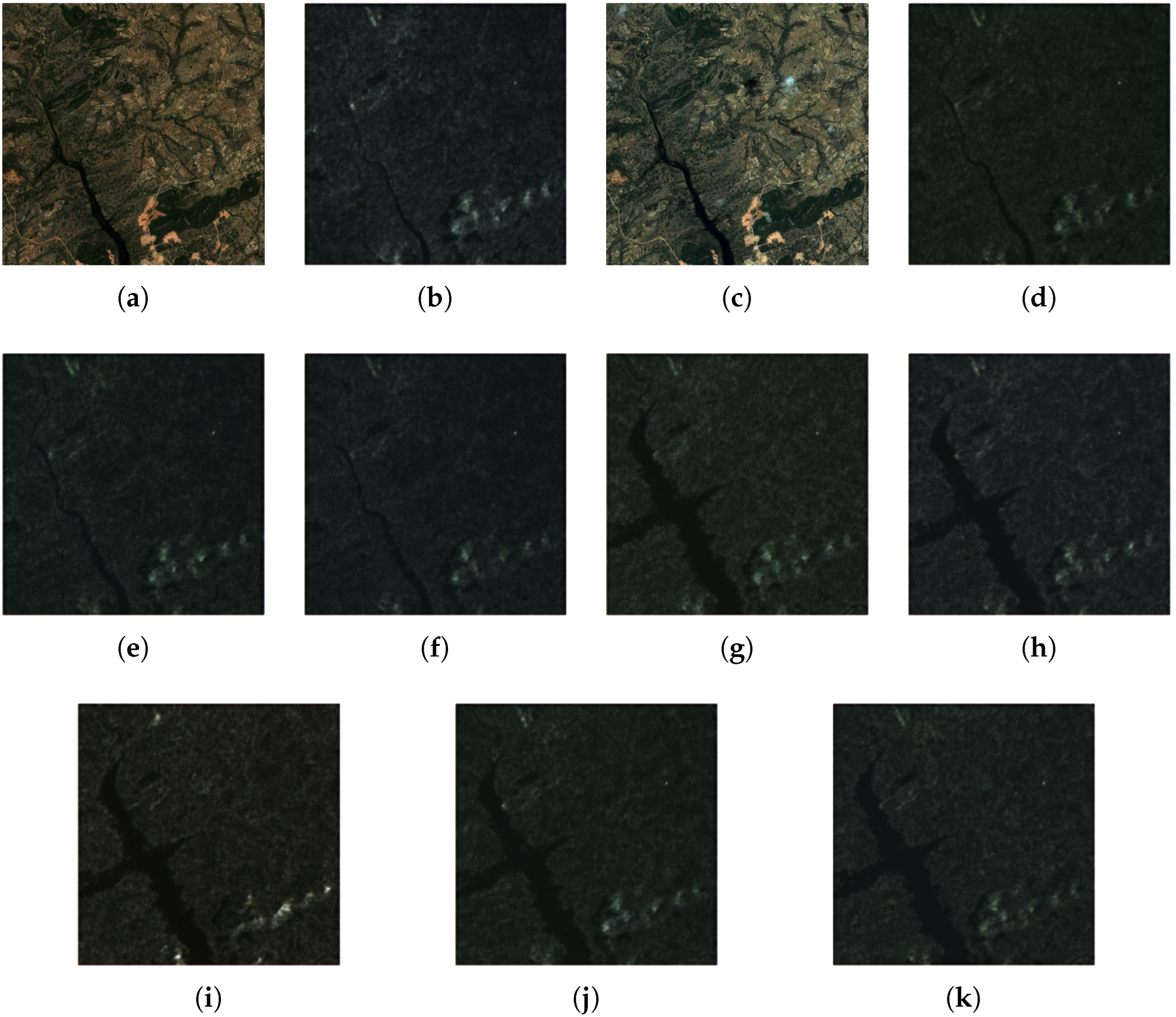
For the second use-case scenario, we considered a landslide that occurred on 15 May 2017 in Alunu, Valcea district, Romania. The landslide destroyed several households and farmlands, roads, and also a forest. The sequence of remote sensing images, shown in Figure 3, is comprised of three optical images and six dual-polarized SAR images of pixels. For the Sentinel-1 images, the images are available in dual-polarization VV + VH, whilst, for the Sentinel-2 images, the visible (B2, B3, B4) bands are considered. In both cases, the bands/polarizations are characterized by 10 m spatial resolution. Similar to the previous dataset [26], these multimodal and multitemporal images have been downloaded from the Copernicus Open-Access Hub [25] and have been preprocessed (including co-registration, radiometric calibration, Range Doppler Terrain Correction) using the Sentinel Application Platform (SNAP) [27], an open software platform provided by the European Space Agency (ESA).
The information for both use-case scenarios is synthesized in Table 1.
2.2. Methodology Overview
Analyzing multimodal SITS is a challenging task. In this paper, we consider a two-stage SITS analysis. The first stage is based on the inter-modality translation of images in SITS, whereas the second stage focuses on detecting hazardous events using the newly introduced concept of matrix profile.
Including an inter-modality translation technique in the image processing pipeline for SITS analysis represents a solution for aligning the images in SITS to the same modality and, afterward, for using standard time series processing algorithms. As summarized in Figure 1, the proposed methodology is formed upon a GAN-based modality translation that maps the SAR images to the optical domain.
Generative Adversarial Networks, GANs, represent a generative framework for estimating new data through an adversarial process [22,28,29]. Two models are trained, namely a generative model that performs the translation from one domain to the other domain and a discriminative model, whose role is to estimate whether the sample comes from the training data or from the generated data. The procedure can be regarded as a game in which the generator tries to produce fake samples that perfectly resemble true samples and thus deceive the discriminator, whereas the discriminator aims to discover the differences between true and generated data.
2.3. GAN-Based Modality-to-Modality Translation
The goal of modality-to-modality translation is to learn inter-domain mapping functions. In our case, the domains are composed of images acquired by a SAR sensor (domain ) and by an optical sensor (domain ), respectively. In the following, we denote by the image acquired by a SAR sensor and by the image acquired by an optical sensor.
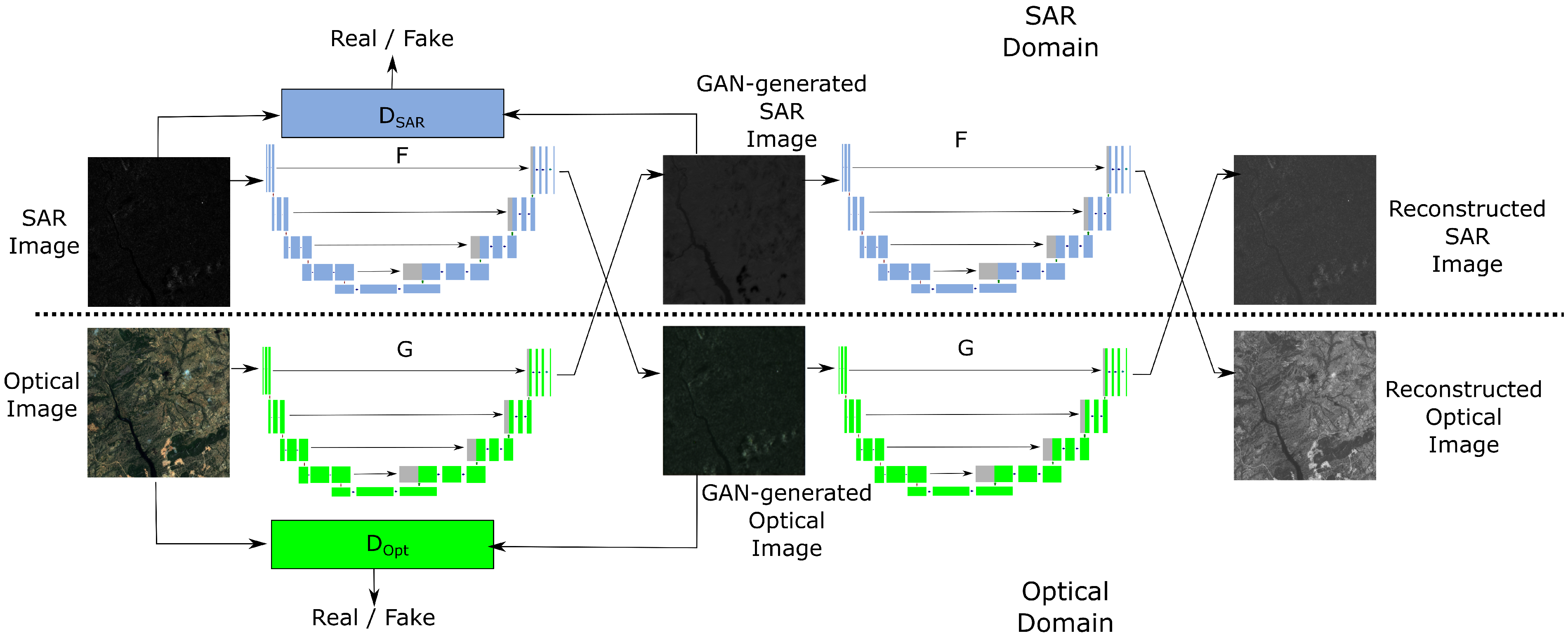
In this work, a model consisting of two mapping functions and , allows the reconstruction of images from one domain to the other. The two generative functions map one domain into the other and thus, the mappings can be applied either to original images or generated ones. More precisely, F can be applied on original SAR images and also on GAN-generated SAR images (i.e., images obtained from optical images by applying the mapping function G). As shown in Figure 4, in addition to the inter-domain mapping functions, we introduce two discriminators, and , for each domain. The role of the discriminators is to distinguish between fake and generated regions.
Considering the structure of the modality-to-modality translation model presented in Figure 4, the objective is composed of three types of loss functions, namely, translation loss, cycle-consistency loss, and adversarial loss. The loss functions will be detailed in the following subsections.
2.3.1. Translation Loss
Considering the task of inter-modality translation, assume that the same location is captured by two sensors characterized by different physical properties, e.g., SAR and optical sensors. The acquired images are denoted by and . The training set is composed by images reflecting various locations for which pairs of images are available. A correct translation from one domain to another is achieved if:
This constraint is expressed through the translation loss term, which tries to map images composing a pair across modalities:
2.3.2. Cycle-Consistency Loss
In order to prevent a possible contradiction between inter-domain mapping functions F and G, Zhu et al. [21] introduced the cycle-consistency loss. Inspired by this approach, in an inter-domain scenario, we impose:
which leads to writing the cycle-consistency loss as:
The cycle-consistency constraint enforces G to act as an inverse mapping for F and vice-versa.
2.3.3. Adversarial Loss
Adversarial networks are discriminative models that learn to determine whether a sample comes from a generated distribution or a true data distribution [28]. Unlike the approach in [28], in this paper, we adopt a least squares loss function for the discriminator instead of the logarithmic one [30,31]. The discriminator should be able to distinguish generated regions (i.e., “fake”) from real regions. We express the adversarial loss as:
where and denote images under CutMix transformations [32]:
with ⊙ representing element-wise multiplication. is a binary mask indicating if the pixel n comes from a real region () or a generated region (). In our setup, CutMix transformations replace rectangular regions from an original image with the corresponding regions taken from the generated image in different mix proportions. This allows a natural augmentation strategy for training the discriminators under limited data, which typically leads to discriminator overfitting [33].
The overall objective is thus:
2.3.4. U-Net-Based Inter-Modality Image Translation
In order to achieve inter-domain image translation, we employ a fully convolutional encoder-decoder scheme, more precisely, the popular U-Net architecture, which was first introduced for biomedical image segmentation [34]. Following an information theory-based parallel, the input is passed, during encoding, through a sequence of layers that successively downsamples the input until a bottleneck layer is met. At this point, the process is reversed, and decoding is performed. The bottlenecked information flowing through the decoder part of the “U”-shaped structure is concatenated, at each level, with mirrored information from the encoder’s layers. The information at each layer is mirrored by means of skip connections added between layer i and layer , n being the total number of layers. In this manner, low-level information between the input and output images is translated through these direct connections instead of being discarded by the bottlenecked process. Thus, U-Net-based modality translation brings several advantages, i.e., the inherent property of aligning the structure in the input to the structure in the output [22], the increased stability achieved by means of shortcut connections [9], and also its potential of dealing with a different number of spectral bands at input and output. The last property is particularly useful when dealing with SAR-to-optical image translation.
Considering the above-mentioned advantages, the U-Net architecture is adopted for both the generative functions, i.e., F and G, and the discriminative functions, i.e., and . The standard U-Net architecture consists of a contracting path and an expansive path connected through a bridge of convolutional layers [34]. The contracting path is composed of four blocks, each with two convolutional layers, a ReLU activation function, and a maxpooling layer. At each downsampling step, the number of channels is doubled, i.e., the number of the output channels is 64 for the first block, 128 for the second block, 256 for the third block, and 512 for the fourth block [34]. The bridge is formed by two convolutional layers with 1024 output channels each, followed by a ReLU activation function. The expansive path contains the same number of blocks as the contracting path, each with two convolutional layers, followed by a ReLU activation function. The number of the output channels characterizing each block in the expansive path is halved at each step, whereas the connection between successive blocks is characterized by up-convolutions. The long skip connections mirror, by concatenation, the information from the blocks in the contracting path to the corresponding blocks in the expansive path. In order to match the number of input and output channels with the requirements of our setup, we slightly modify the standard U-Net architecture. Specifically, if and represent the number of bands for the SAR and optical images, respectively, the generative U-Net function F has input channels and output channels, whereas the generative U-Net function G has input channels and output channels. Similarly, the discriminators follow a U-Net architecture, with and input channels (i.e., depending on the domain) and one output channel. Since the translation is performed from the SAR domain to the optical domain, the resulting SITS is composed of original and generated optical images, all being characterized by a number of spectral bands.
2.4. Identification of Anomalies in a Change Detection Framework for Multimodal SITS
In the previous section, the multimodal SITS has been translated into a SITS formed by original optical images and “fake” optical images, i.e., images obtained from SAR images by applying a modality-to-modality translation. In this way, the resulting SITS are composed of temporal sequences of length N, and each sample in the sequence has components (i.e., the number of spectral bands of the optical sensor). N represents the number of images that form the SITS, i.e., original or generated. In the following, we propose an approach toward the identification of abnormal events under a more general framework for multimodal time-series change detection.
2.4.1. Detection of Abnormal Events in SITS
We adopt an all-pairs-similarity-search (or similarity join) approach for the identification of time series differences. All-pairs similarity search algorithms are considered to be very competitive as novelty and anomaly detectors [24,35], whereas in terms of motif and novelty discovery tasks, one of the fastest algorithms used for finding similarity joins between time series subsequences is the matrix profile, described in [24].
Let us consider a time series x of length N, i.e., the time series x is composed of N pixel arrays at the same position in the SITS. The similarity joins are searched in an all-subsequences set of the time series, which is composed of all the subsequences of a given length m, which are obtained by sliding a window over the time series x. Specifically, given a query of length m, the nearest neighbor (NN) is searched among all the possible subsequences of x of length m. In the following, we denote by the subsequence of length m starting at sample and by the subsequence of length m starting at sample . The similarity join set records, in an ordered manner, pairs of the form , where is the nearest neighbor of in terms of Euclidian distance.
Apart from being fast in discovering similarity joins, the matrix profile algorithm is parameter-free. With a slight modification of the initial concept of matrix profile [24], we can extend the concept to C-dimensional signals, where C denotes the number of spectral bands in the newly created SITS (i.e., containing original and generated optical images with spectral bands). More specifically, for each pair of the similarity join set, we store the squared Euclidian distance between the C-dimensional temporal subsequence of length m, , and the corresponding nearest neighbor, i.e., :
where denotes the value that corresponds to channel c of sample .
The matrix profile accompanies each spatio-temporal sequence in SITS, and a relatively high value in the matrix profile of a sequence corresponds to a difference or anomaly. More precisely, a subsequence in the original temporal sequence that is unique in its shape is characterized by a high value of [24]. Specifically, a time series difference is a subsequence that is most dissimilar to its nearest neighbor subsequence. Therefore, the identification of anomalies, or differences, in a time series x reduces to recording the highest values in the corresponding matrix profile:
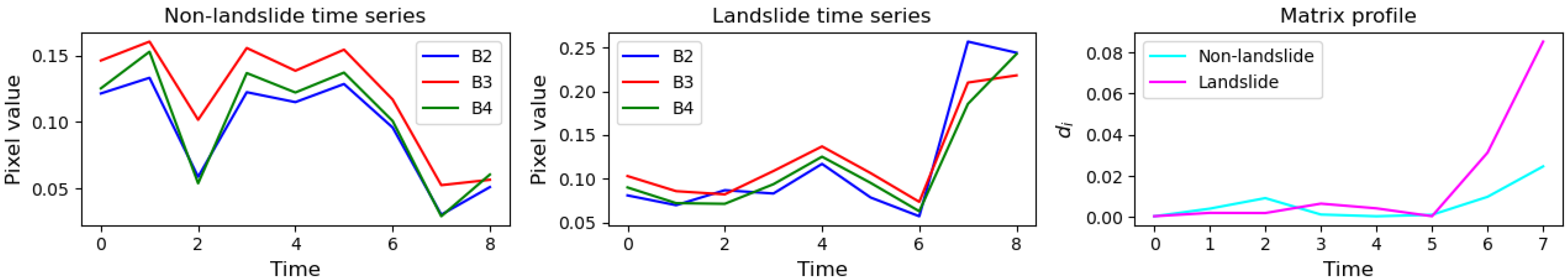
The value is an indicator of the relevance of an anomalous event, whereas the examination of the matrix profile reveals the change point or the moment an anomaly occurs. This can be observed in Figure 5, where two time series are shown, one corresponding to a “normal” time series, whilst the second one is extracted from a region where an anomalous event (i.e., landslide) occurred.
2.4.2. Unsupervised Change Detection in a Maximum-Likelihood Estimation Framework
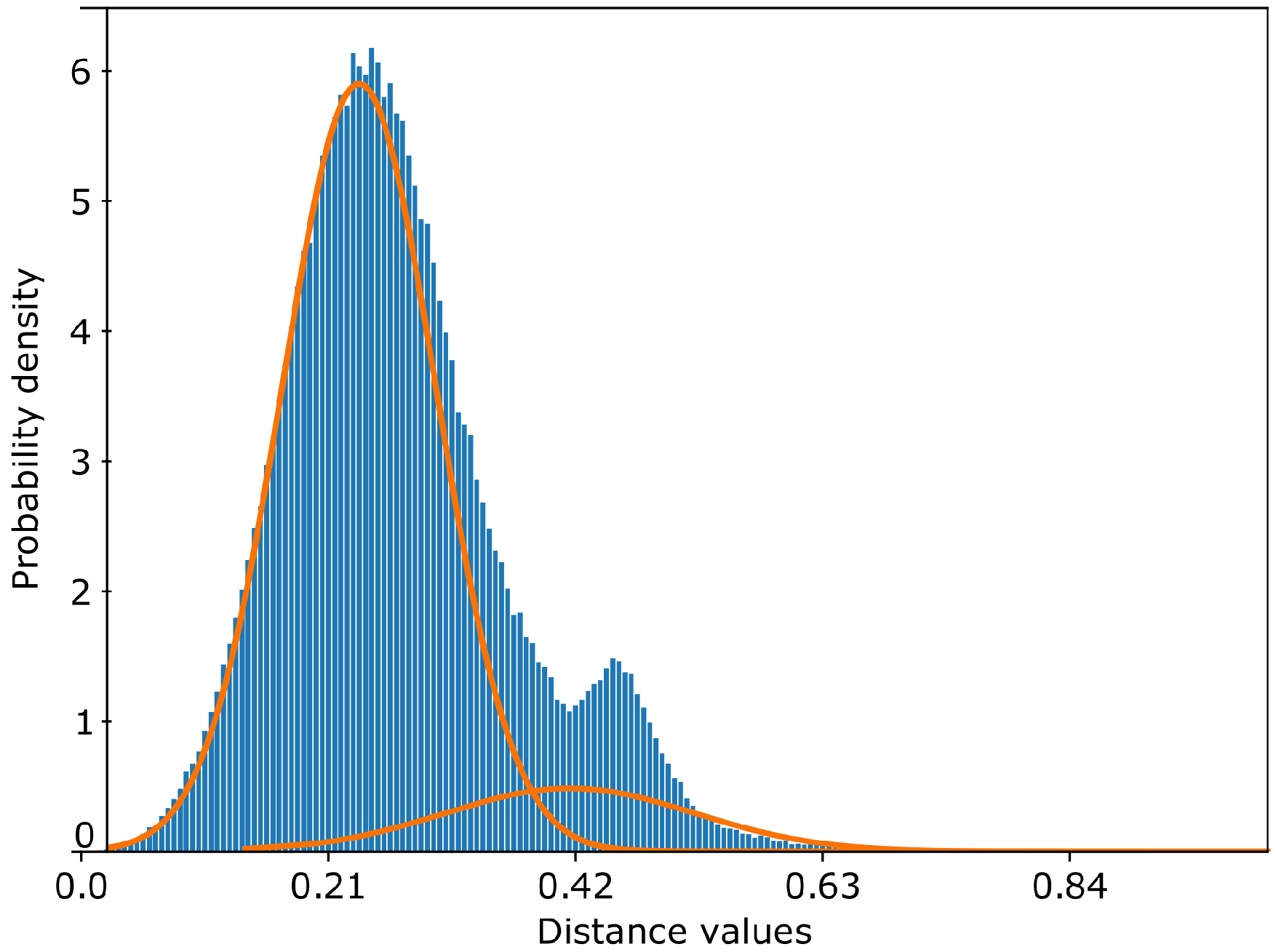
In order to identify the anomalies in SITS, we form a new image from the maximum matrix profile values extracted for each pixel. Intuitively, the higher the maximum value in the matrix profiles of spatio-temporal sequences, the more significant the difference/anomaly is. In this regard, the optimal threshold that separates an abnormal event from the rest of the spatio-temporal events in SITS can be determined following an Expectation-Maximization (EM)-based thresholding technique [36].
As shown in Figure 6, the histogram over the maximum matrix profile values follows a mixture of two Gaussian distributions, one corresponding to regions containing anomalies, whereas the other to unchanged regions. Thus, assuming that the maximum value of a matrix profile that accompanies a spatio-temporal sequence is taken from a mixture of two Gaussian distributions, (i.e., corresponding to regions containing anomalies) and (i.e., corresponding to unchanged regions), we can write the posterior probability as:
where are the model parameters. Specifically, and are the mixture probabilities such that , whilst and are the mean and standard deviations that correspond to the two Gaussian distributions.
Following the Maximum-Likelihood Estimation (MLE) framework, the goal is to estimate the model parameters such that the log-likelihood is maximized:
The Expectation-Maximization technique allows the estimation of the aforementioned model parameters in an iterative manner (i.e., from iteration t to next iteration ) [13]:
where , H and W are the height and the width of the images in SITS, and values are derived as:
After the estimation of the model parameters, the optimal threshold that separates the two classes (i.e., anomaly and unchanged) are determined from the equality:
which as shown in [13] leads to a quadratic equation in . The equation has two possible solutions, but only one solution is between and . This solution represents the optimal threshold that outlines the anomaly in SITS, i.e., if is greater than the threshold , then corresponds to an anomaly.
3. Experiments
3.1. Inter-Modality Translation
The inter-modality translation model was trained on 500 pairs of Sentinel-1 and Sentinel-2 patches with dimensions of pixels randomly selected from the datasets. However, since the changes occurring between two different moments of time may distort the learning process, we selected images that were captured at close temporal moments and that were not interfering with the areas affected by the hazardous events. As mentioned, the loss function incorporates a translation loss, a cycle-consistency loss, and an adversarial loss term, with corresponding weights , , and , respectively. In addition, we added a regularization term with a weight decay of 0.001, which controls the magnitude of the network parameters and reduces overfitting. During the training procedure, we used the Stochastic Gradient Descent (SGD) optimization algorithm, with momentum set to 0.9. The model was trained for 250 epochs, with a batch size of 8 and a learning rate of . In Figure 7 and Figure 8, we present the results of the GAN-based inter-modality translation for the two datasets of Sentinel-1 and Sentinel-2 images described in Section 2.1.
3.2. Performance Evaluation for Multimodal Time-Series Change Detection
In order to detect anomalies caused by natural disasters (e.g., flooding, landslide), we use a time-series change detection framework based on a modified matrix profile concept. Since the detection of a natural disaster at a certain moment of time involves the analysis of a pre-event image and a post-event image, we set the length of the subsequences m to 2. This assumption leads to quantifying whether regions captured at consecutive moments of time experience a major event or not. If a natural disaster occurs, this anomaly will be reflected by the high values in the matrix profile accompanying the corresponding time series in SITS. The optimal threshold in the matrix of maximum matrix profile values is determined via the EM algorithm, whose initialization is performed by using the K-Means algorithm.
The performance of the proposed algorithm, GAN-MP, for multimodal time-series change detection is measured in terms of overall accuracy (), true negative rate (), true positive rate (), and F-score, which were computed as:
where , and stand for true positives, true negatives, false positives, and false negatives, respectively.
4. Discussion
The projections from the SAR to the optical domain yield a mono-modal SITS, containing both original and generated optical images. Using the U-Net architecture for inter-modality translation in a GAN-based setup, the generated optical images will have the same number of spectral bands and also similar characteristics to the original optical images. The proposed approach for multimodal SITS analysis, GAN-MP, is based on the matrix profile concept and allows the retrieval of anomalies in heterogeneous SITS. In Figure 9a and Figure 10a, the matrix of values indicates the regions where an anomaly or hazardous event occurred, in the sense that, as expected, these regions exhibit higher values of . Comparing the qualitative results presented in Figure 9b and Figure 10b to the corresponding ground-truth images, the EM algorithm effectively delimits the affected regions by determining the optimal threshold that is applied over the values. From a quantitative point of view, the performance results are summarized in Table 2, and, in both cases, the proposed technique achieves an overall accuracy greater than 96%.
Most of the SITS analysis methods, e.g., unsupervised clustering of SITS, are designed for mono-modal remote sensing images. Since the acquisitions in a mono-modal setup are performed using the same sensor, the spatio-temporal evolutions can be clustered using standard methods, e.g., the DTW distance measure can be used in conjunction with the K-Means algorithm, yielding an unsupervised clustering of spatio-temporal evolutions in SITS [5,7]. Moreover, the mono-modal SITS can be analyzed using standard techniques, e.g., the Latent Dirichlet Allocation (LDA) model to extract latent information from the scene or DTW and EM to retrieve similar evolution patterns [36]. In the case of multimodal SITS, the application of these mono-modal SITS analysis techniques is possible if a projection of the images from another modality to the current modality of analysis is performed beforehand.
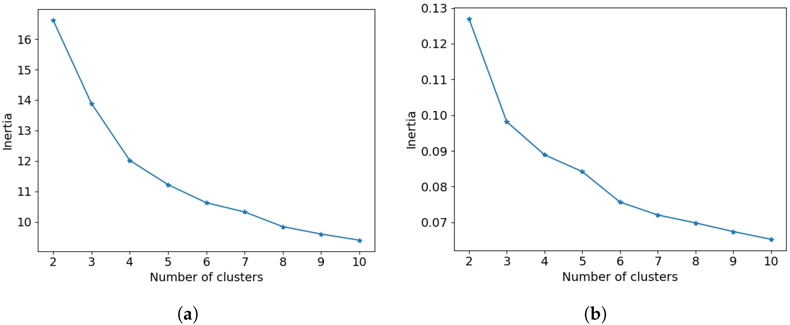
In Figure 9d and Figure 10d, we show the results obtained by applying the DTW-based K-means clustering method [5,7] on SITS formed by original and translated optical images in both use-case scenarios, e.g., flooding and landslide. The number of clusters has been set using the Elbow method, which determines the optimal number of clusters by analyzing the shape of the cost function (or inertia) [37]. In the case of K-means clustering, the cost function is the sum of within-cluster distances, i.e., distances from points to the closest cluster centroids. Considering that the K-means for SITS clustering uses the DTW distance measure, we replace the Euclidean distance in the cost function with the DTW distance measure. The cost function with respect to the number of clusters is shown in Figure 11. In the case of the flooding event, the Elbow point (i.e., the point after which the decrease in the cost function with the number of clusters becomes slow or linear) is 4, whereas, in the case of the landslide event, the optimal number of clusters is 5. With these parameters set, Figure 9d and Figure 10d represent the DTW-based K-Means clustering for the two use-case scenarios. Although both the flooding and the landslide events form a distinct category of spatio-temporal evolutions, the unsupervised clustering of spatio-temporal evolutions does not provide information regarding either the possible occurrence of an anomaly or the specific class incorporating the anomaly. In this regard, the retrieval of spatio-temporal events that are similar to a given query, e.g., a single spatio-temporal sequence provided by the user, can be performed using the DTW distance measure computed between all the spatio-temporal sequences in the SITS and the given query [36]. The separation between similar and non-similar patterns is obtained using the EM technique, as shown in Figure 9e and Figure 10e [36].
Apart from the above-mentioned methods, we investigate adversarial cyclic encoder networks, which have been recently proposed in [10] for image translation in an unsupervised multimodal change detection framework. During the experiments, we follow the same architecture and setup as in the original paper, whereas the threshold over the distance image is automatically determined via Otsu’s method [10]. Considering the first and last images in SITS as the pre-event and the post-event images, the delimitation of the landslide event is clear in Figure 10f. In the flooding use-case scenario, the delimitation of the event is less accurate.
Finally, Table 2 shows the results achieved by the proposed technique and detailed quantitative comparisons for the two considered multimodal SITS. In both use-case scenarios, the existence of multitemporal information has an important impact over the performance of the algorithms. In this regard, the results show that considering only pre-event and post-event images leads to an increased number of false alarms, e.g., Figure 9f and Figure 10f.
5. Conclusions
This paper describes a new approach toward unsupervised multimodal SITS analysis. SITS composed of images acquired by different sensors are brought into the same modality domain by means of an inter-modality translation technique, which follows a GAN-based architecture. Working in the same domain allows the usage of standard techniques for analyzing spatio-temporal evolutions in SITS, e.g., DTW-based K-means clustering. In order to detect anomalies and analyze the consequences of natural hazards, we introduce a similarity search methodology based on the extension of the matrix profile concept to SITS analysis. Finally, the identification of regions affected by natural hazards is based on an optimal thresholding approach defined in an MLE framework. Experiments were conducted on two datasets that contain multimodal and multitemporal remote sensing images in two use-case scenarios, namely, flooding and landslide events. The experimental results show the effectiveness of the proposed framework in terms of the delimitation of the regions affected by natural hazards, which further allows a better assessment of the damage caused by these natural events. In this regard, the performance in terms of overall accuracy exceeds 96 % in both use-case scenarios. Moreover, the experimental results establish the importance of multitemporal information when dealing with anomaly detection in SITS, whilst the matrix profile concept allows the identification of the change point corresponding to the occurrence of a hazardous event.
Funding
This work was supported by a grant of the Romanian Ministry of Education and Research, CNCS-UEFISCDI, project number PN-III-P1-1.1-PD-2019-0843 (MDM-SITS), within PNCDI III.
Data Availability Statement
Not applicable.
Acknowledgments
The author would like to thank: my students, Teodora Pinzariu and Marina Barbu, for selecting relevant remote sensing images for the landslide detection use-case scenario, Mihai Datcu (DLR, Germany) for providing access to the SEN12-FLOOD dataset, and Bogdan Ionescu (University Politehnica of Bucharest, Romania) for support during the project’s implementation.
Conflicts of Interest
The author declares no conflict of interest.
Abbreviations
The following abbreviations are used in this manuscript:
| EO | Earth Observation |
| SITS | Satellite Image Time Series |
| SAR | Synthetic Aperture Radar |
| GAN | Generative Adversarial Network |
| CNN | Convolutional Neural Network |
| MLE | Maximum Likelihood Estimation |
| EM | Expectation Maximization |
| DTW | Dynamic Time Warping |
References
- Simoes, R.; Camara, G.; Queiroz, G.; Souza, F.; Andrade, P.R.; Santos, L.; Carvalho, A.; Ferreira, K. Satellite Image Time Series Analysis for Big Earth Observation Data. Remote Sens. 2021, 13, 2428. [Google Scholar] [CrossRef]
- Zhao, C.; Lu, Z. Remote Sensing of Landslides—A Review. Remote Sens. 2018, 10, 279. [Google Scholar] [CrossRef] [Green Version]
- Zhao, Y.; Celik, T.; Liu, N.; Li, H.C. A Comparative Analysis of GAN-Based Methods for SAR-to-Optical Image Translation. IEEE Geosci. Remote Sens. Lett. 2022, 19, 1–5. [Google Scholar] [CrossRef]
- Barbu, M.; Radoi, A.; Suciu, G. Landslide Monitoring using Convolutional Autoencoders. In Proceedings of the 2020 12th International Conference on Electronics, Computers and Artificial Intelligence (ECAI), Bucharest, Romania, 25–27 June 2020; pp. 1–6. [Google Scholar] [CrossRef]
- Petitjean, F.; Inglada, J.; Gancarski, P. Satellite Image Time Series Analysis Under Time Warping. IEEE Trans. Geosci. Remote Sens. 2012, 50, 3081–3095. [Google Scholar] [CrossRef]
- Prendes, J.; Chabert, M.; Pascal, F.; Giros, A.; Tourneret, J.Y. Performance assessment of a recent change detection method for homogeneous and heterogeneous images. Rev. Française Photogrammétrie Télédétection 2015, 209, 23–29. [Google Scholar] [CrossRef]
- Petitjean, F.; Forestier, G.; Webb, G.I.; Nicholson, A.E.; Chen, Y.; Keogh, E. Dynamic Time Warping Averaging of Time Series Allows Faster and More Accurate Classification. In Proceedings of the 2014 IEEE International Conference on Data Mining, Shenzhen, China, 14–17 December 2014; pp. 470–479. [Google Scholar] [CrossRef] [Green Version]
- Yan, J.; Wang, L.; He, H.; Liang, D.; Song, W.; Han, W. Large-Area Land-Cover Changes Monitoring With Time-Series Remote Sensing Images Using Transferable Deep Models. IEEE Trans. Geosci. Remote Sens. 2022, 60, 1–17. [Google Scholar] [CrossRef]
- Liu, X.; Hong, D.; Chanussot, J.; Zhao, B.; Ghamisi, P. Modality Translation in Remote Sensing Time Series. IEEE Trans. Geosci. Remote Sens. 2022, 60, 1–14. [Google Scholar] [CrossRef]
- Luppino, L.T.; Kampffmeyer, M.; Bianchi, F.M.; Moser, G.; Serpico, S.B.; Jenssen, R.; Anfinsen, S.N. Deep Image Translation With an Affinity-Based Change Prior for Unsupervised Multimodal Change Detection. IEEE Trans. Geosci. Remote Sens. 2022, 60, 1–22. [Google Scholar] [CrossRef]
- Luppino, L.T.; Hansen, M.A.; Kampffmeyer, M.; Bianchi, F.M.; Moser, G.; Jenssen, R.; Anfinsen, S.N. Code-Aligned Autoencoders for Unsupervised Change Detection in Multimodal Remote Sensing Images. IEEE Trans. Neural Netw. Learn. Syst. 2022, 1–13. [Google Scholar] [CrossRef]
- Maggiolo, L.; Solarna, D.; Moser, G.; Serpico, S.B. Registration of Multisensor Images through a Conditional Generative Adversarial Network and a Correlation-Type Similarity Measure. Remote Sens. 2022, 14, 2811. [Google Scholar] [CrossRef]
- Bruzzone, L.; Prieto, D.F. Automatic analysis of the difference image for unsupervised change detection. IEEE Trans. Geosci. Remote Sens. 2000, 38, 1171–1182. [Google Scholar] [CrossRef] [Green Version]
- Radoi, A.; Datcu, M. Automatic Change Analysis in Satellite Images Using Binary Descriptors and Lloyd-Max Quantization. IEEE Geosci. Remote Sens. Lett. 2015, 12, 1223–1227. [Google Scholar] [CrossRef] [Green Version]
- Touati, R.; Mignotte, M.; Dahmane, M. Change Detection in Heterogeneous Remote Sensing Images Based on an Imaging Modality-Invariant MDS Representation. In Proceedings of the 2018 25th IEEE International Conference on Image Processing (ICIP), Athens, Greece, 7–10 October 2018; pp. 3998–4002. [Google Scholar] [CrossRef]
- Liu, Z.; Li, G.; Mercier, G.; He, Y.; Pan, Q. Change Detection in Heterogenous Remote Sensing Images via Homogeneous Pixel Transformation. IEEE Trans. Image Process. 2018, 27, 1822–1834. [Google Scholar] [CrossRef] [PubMed]
- Luppino, L.T.; Bianchi, F.M.; Moser, G.; Anfinsen, S.N. Unsupervised Image Regression for Heterogeneous Change Detection. IEEE Trans. Geosci. Remote Sens. 2019, 57, 9960–9975. [Google Scholar] [CrossRef] [Green Version]
- Mignotte, M. A Fractal Projection and Markovian Segmentation-Based Approach for Multimodal Change Detection. IEEE Trans. Geosci. Remote Sens. 2020, 58, 8046–8058. [Google Scholar] [CrossRef]
- Liu, J.; Gong, M.; Qin, K.; Zhang, P. A Deep Convolutional Coupling Network for Change Detection Based on Heterogeneous Optical and Radar Images. IEEE Trans. Neural Netw. Learn. Syst. 2018, 29, 545–559. [Google Scholar] [CrossRef]
- Zhang, P.; Gong, M.; Su, L.; Liu, J.; Li, Z. Change detection based on deep feature representation and mapping transformation for multi-spatial-resolution remote sensing images. ISPRS J. Photogramm. Remote Sens. 2016, 116, 24–41. [Google Scholar] [CrossRef]
- Zhu, J.Y.; Park, T.; Isola, P.; Efros, A.A. Unpaired Image-to-Image Translation Using Cycle-Consistent Adversarial Networks. In Proceedings of the IEEE International Conf. on Computer Vision (ICCV), Venice, Italy, 22–29 October 2017; pp. 2242–2251. [Google Scholar] [CrossRef] [Green Version]
- Isola, P.; Zhu, J.Y.; Zhou, T.; Efros, A.A. Image-to-Image Translation with Conditional Adversarial Networks. In Proceedings of the IEEE Conference on Computer Vision and Pattern Recognition (CVPR), Honolulu, HI, USA, 21–26 July 2017; pp. 5967–5976. [Google Scholar] [CrossRef] [Green Version]
- Benedetti, P.; Ienco, D.; Gaetano, R.; Ose, K.; Pensa, R.G.; Dupuy, S. M3Fusion: A Deep Learning Architecture for Multiscale Multimodal Multitemporal Satellite Data Fusion. IEEE J. Sel. Top. Appl. Earth Obs. Remote Sens. 2018, 11, 4939–4949. [Google Scholar] [CrossRef] [Green Version]
- Yeh, C.C.M.; Zhu, Y.; Ulanova, L.; Begum, N.; Ding, Y.; Dau, H.A.; Silva, D.F.; Mueen, A.; Keogh, E. Matrix Profile I: All Pairs Similarity Joins for Time Series: A Unifying View That Includes Motifs, Discords and Shapelets. In Proceedings of the 2016 IEEE 16th International Conference on Data Mining (ICDM), Barcelona, Spain, 12–15 December 2016; pp. 1317–1322. [Google Scholar] [CrossRef]
- Copernicus Open Access Hub. Available online: https://scihub.copernicus.eu/ (accessed on 1 September 2020).
- Rambour, C.; Audebert, N.; Koeniguer, E.; Le Saux, B.; Crucianu, M.; Datcu, M. Flood Detection in the Time Series of Optical and SAR Images. Int. Arch. Photogramm. Remote Sens. Spat. Inf. Sci. 2020, XLIII-B2-2020, 1343–1346. [Google Scholar] [CrossRef]
- SNAP-ESA Sentinel Application Platform. Available online: http://step.esa.int/ (accessed on 1 September 2020).
- Goodfellow, I.; Pouget-Abadie, J.; Mirza, M.; Xu, B.; Warde-Farley, D.; Ozair, S.; Courville, A.; Bengio, Y. Generative Adversarial Nets. In Proceedings of the Advances in Neural Information Processing Systems; Ghahramani, Z., Welling, M., Cortes, C., Lawrence, N., Weinberger, K., Eds.; Curran Associates, Inc.: Montreal, QC, Canada, 2014; Volume 27. [Google Scholar]
- Pathak, D.; Krähenbühl, P.; Donahue, J.; Darrell, T.; Efros, A.A. Context Encoders: Feature Learning by Inpainting. In Proceedings of the 2016 IEEE Conference on Computer Vision and Pattern Recognition (CVPR), Las Vegas, NV, USA, 27–30 June 2016; pp. 2536–2544. [Google Scholar] [CrossRef] [Green Version]
- Mao, X.; Li, Q.; Xie, H.; Lau, R.Y.; Wang, Z.; Smolley, S.P. Least Squares Generative Adversarial Networks. In Proceedings of the IEEE International Conference on Computer Vision (ICCV), Venice, Italy, 22–29 October 2017; pp. 2813–2821. [Google Scholar] [CrossRef] [Green Version]
- Kurach, K.; Lučić, M.; Zhai, X.; Michalski, M.; Gelly, S. A Large-Scale Study on Regularization and Normalization in GANs. In Proceedings of the International Conference on Machine Learning, Long Beach, CA, USA, 9–15 June 2019. [Google Scholar]
- Yun, S.; Han, D.; Oh, S.J.; Chun, S.; Choe, J.; Yoo, Y.J. CutMix: Regularization Strategy to Train Strong Classifiers With Localizable Features. IEEE/CVF Int. Conf. Comput. Vis. (ICCV) 2019, 6022–6031. [Google Scholar] [CrossRef] [Green Version]
- Karras, T.; Aittala, M.; Hellsten, J.; Laine, S.; Lehtinen, J.; Aila, T. Training Generative Adversarial Networks with Limited Data. Proc. Adv. Neural Inf. Process. Syst. 2020, 33, 12104–12114. [Google Scholar]
- Ronneberger, O.; Fischer, P.; Brox, T. U-net: Convolutional networks for biomedical image segmentation. In Proceedings of the International Conference on Medical image Computing and Computer-Assisted Intervention, Munich, Germany, 5–9 October 2015; Springer: Berlin/Heidelberg, Germany, 2015; pp. 234–241. [Google Scholar]
- Chandola, V.; Cheboli, D.; Kumar, V. Detecting Anomalies in a Time Series Database; Technical Report; University of Minnesota Digital Conservancy: Minneapolis, MN, USA, 2009; Volume UMN TR 09-004. [Google Scholar]
- Radoi, A.; Burileanu, C. Retrieval of Similar Evolution Patterns from Satellite Image Time Series. Appl. Sci. 2018, 8, 2435. [Google Scholar] [CrossRef] [Green Version]
- Liu, F.; Deng, Y. Determine the Number of Unknown Targets in Open World Based on Elbow Method. IEEE Trans. Fuzzy Syst. 2021, 29, 986–995. [Google Scholar] [CrossRef]
Figure 1.
Methodology overview for multi-source SITS analysis. The images with a dashed border represent the corresponding GAN-based translations of images from the second modality.
Figure 1.
Methodology overview for multi-source SITS analysis. The images with a dashed border represent the corresponding GAN-based translations of images from the second modality.

Figure 2.
Mixed Sentinel-1 and Sentinel-2 SITS for flood detection: (a) 1 February 2019 (Sentinel-2), (b) 4 February 2019 (Sentinel-1), (c) 11 February 2019 (Sentinel-2), (d) 16 February 2019 (Sentinel-1), (e) 28 February 2019 (Sentinel-1), (f) 12 March 2019 (Sentinel-1), (g) 18 March 2019 (Sentinel-1), (h) 24 March 2019 (Sentinel-1), (i) 30 March 2019 (Sentinel-1), (j) 5 April 2019 (Sentinel-1), (k) 17 April 2019 (Sentinel-1).

Figure 3.
Mixed Sentinel-1 and Sentinel-2 SITS for landslide detection: (a) 18 December 2016 (Sentinel-1), (b) 30 December 2016 (Sentinel-1), (c) 9 April 2017 (Sentinel-2), (d) 10 April 2017 (Sentinel-1), (e) 11 May 2017 (Sentinel-1), (f) 16 June 2017 (Sentinel-1), (g) 22 July 2017 (Sentinel-1), (h) 27 August 2017 (Sentinel-2), (i) 16 October 2017 (Sentinel-2).

Figure 4.
GAN-based image-to-image translation.

Figure 5.
Example of time series in SITS. The first time series corresponds to a non-landslide region, whereas the second time series is extracted from the region where the landslide occurred. The matrix profile exhibit higher values for the time series that correspond to the landslide. Moreover, the change point (i.e., sample number 5) retrieved from the matrix profile corresponds to the immediate acquisition moment after the landslide occurred, i.e., 16 June 2017.

Figure 6.
Histogram over maximum matrix profile values and a mixture of two Gaussian distributions fitted to these values. The first Gaussian corresponds to pixels from the unchanged regions, whereas the second one corresponds to pixels from regions affected by anomalous events.
Figure 6.
Histogram over maximum matrix profile values and a mixture of two Gaussian distributions fitted to these values. The first Gaussian corresponds to pixels from the unchanged regions, whereas the second one corresponds to pixels from regions affected by anomalous events.

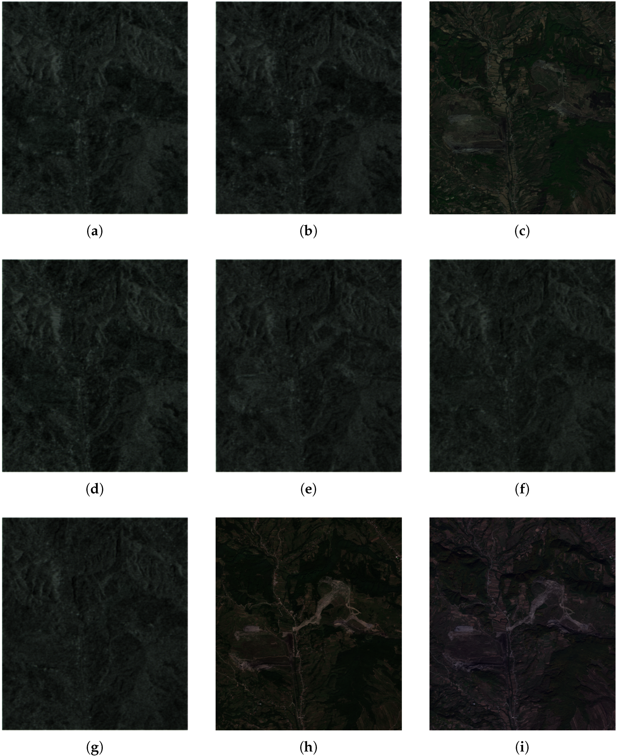
Figure 7.
Original and generated SITS in the optical domain: (a) 1 February 2019, (b) 4 February 2019, (c) 11 February 2019, (d) 16 February 2019, (e) 28 February 2019, (f) 12 March 2019, (g) 18 March 2019, (h) 24 March 2019, (i) 30 March 2019, (j) 5 April 2019, (k) 17 April 2019.
Figure 7.
Original and generated SITS in the optical domain: (a) 1 February 2019, (b) 4 February 2019, (c) 11 February 2019, (d) 16 February 2019, (e) 28 February 2019, (f) 12 March 2019, (g) 18 March 2019, (h) 24 March 2019, (i) 30 March 2019, (j) 5 April 2019, (k) 17 April 2019.

Figure 8.
Original and generated SITS in the optical domain for landslide detection: (a) 18 December 2016, (b) 30 December 2016, (c) 9 April 2017, (d) 10 April 2017, (e) 11 May 2017, (f) 16 June 2017, (g) 22 July 2017, (h) 27 August 2017, (i) 16 October 2017.
Figure 8.
Original and generated SITS in the optical domain for landslide detection: (a) 18 December 2016, (b) 30 December 2016, (c) 9 April 2017, (d) 10 April 2017, (e) 11 May 2017, (f) 16 June 2017, (g) 22 July 2017, (h) 27 August 2017, (i) 16 October 2017.

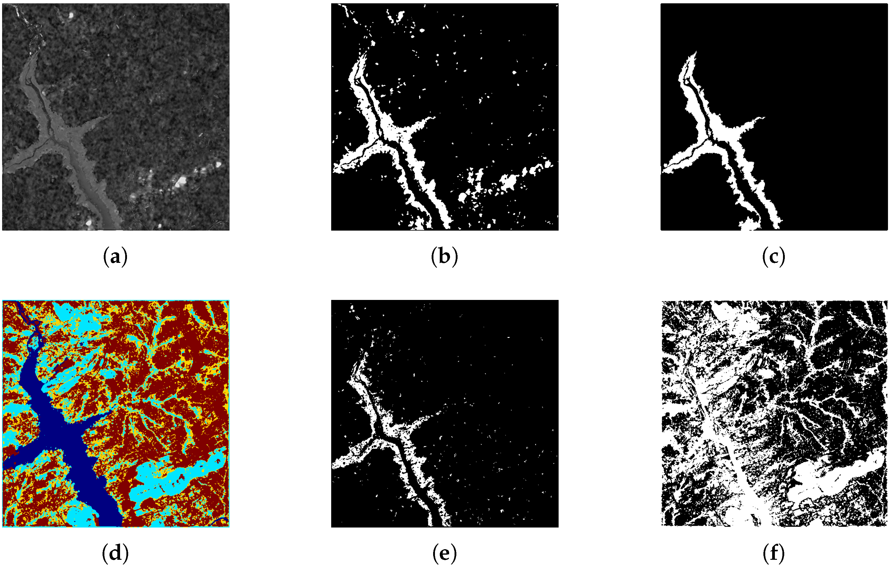
Figure 9.
Anomaly detection in SITS—flooding use-case scenario. From left to right: (a) matrix of values, (b) anomaly identification using the proposed approach, (c) ground truth, (d) DTW-based clustering of heterogeneous SITS using the approach proposed in Ref. [5], (e) retrieval of similar evolution patterns in heterogeneous SITS using DTW-EM method described in Ref. [36], and (f) change map obtained using ACE-Net presented in Ref. [10].

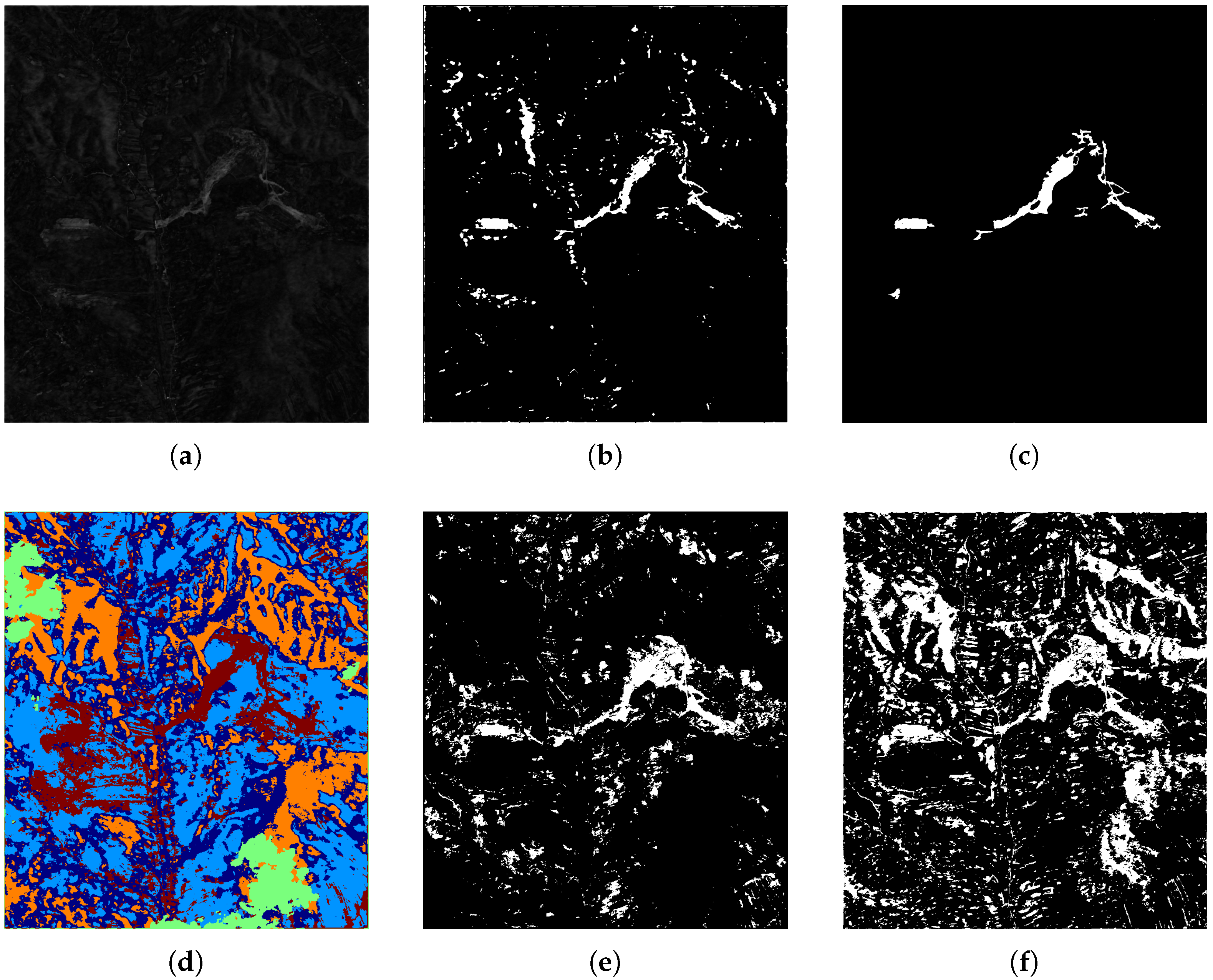
Figure 10.
Anomaly detection in SITS—landslide use-case scenario. From left to right: (a) matrix of values, (b) anomaly identification using the EM-based approach, (c) ground truth, (d) DTW-based clustering of heterogeneous SITS using the approach proposed in Ref. [5], (e) retrieval of similar evolution patterns in heterogeneous SITS using DTW-EM described in Ref. [36], and (f) change map using ACE-Net presented in Ref. [10].

Figure 11.
Determining the optimal number of clusters using the Elbow method for both use-case scenarios, namely (a) flooding and (b) landslide.
Figure 11.
Determining the optimal number of clusters using the Elbow method for both use-case scenarios, namely (a) flooding and (b) landslide.


Table 1.
Use-case scenarios.
| Event | Location | Monitoring Period | Number of Images in SITS | Image Dimensions |
|---|---|---|---|---|
| Flooding | BuheraZimbabwe | 1 February 2019–17 April 2019 | 9 Sentinel-12 Sentinel-2 | |
| Landslide | AlunuRomania | 18 December 2016–6 October 2017 | 6 Sentinel-13 Sentinel-2 |
Table 2.
Performance evaluation and comparisons with other approaches.
| Event | Method | Overall Accuracy | True Positive Rate | True Negative Rate | F-Score |
|---|---|---|---|---|---|
| Flooding | Proposed GAN-MP | 96.59% | 92.29% | 96.93% | 0.79 |
| DTW-EM [36] | 95.26% | 56.21% | 98.37% | 0.64 | |
| ACE-Net [10] | 61.64% | 65.38% | 61.34% | 0.20 | |
| Landslide | Proposed GAN-MP | 97.18% | 80.68% | 97.46% | 0.49 |
| DTW-EM [36] | 93.05% | 85.75% | 93.18% | 0.29 | |
| ACE-Net [10] | 80.66% | 87.67% | 80.53% | 0.13 |
Publisher’s Note: MDPI stays neutral with regard to jurisdictional claims in published maps and institutional affiliations. |
© 2022 by the author. Licensee MDPI, Basel, Switzerland. This article is an open access article distributed under the terms and conditions of the Creative Commons Attribution (CC BY) license (https://creativecommons.org/licenses/by/4.0/).
Share and Cite
MDPI and ACS Style
Radoi, A. Multimodal Satellite Image Time Series Analysis Using GAN-Based Domain Translation and Matrix Profile. Remote Sens. 2022, 14, 3734. https://0-doi-org.brum.beds.ac.uk/10.3390/rs14153734
AMA Style
Radoi A. Multimodal Satellite Image Time Series Analysis Using GAN-Based Domain Translation and Matrix Profile. Remote Sensing. 2022; 14(15):3734. https://0-doi-org.brum.beds.ac.uk/10.3390/rs14153734
Chicago/Turabian StyleRadoi, Anamaria. 2022. "Multimodal Satellite Image Time Series Analysis Using GAN-Based Domain Translation and Matrix Profile" Remote Sensing 14, no. 15: 3734. https://0-doi-org.brum.beds.ac.uk/10.3390/rs14153734
Note that from the first issue of 2016, this journal uses article numbers instead of page numbers. See further details here.