Deep Learning for Mapping Tropical Forests with TanDEM-X Bistatic InSAR Data

Abstract

The TanDEM-X synthetic aperture radar (SAR) system allows for the recording of bistatic interferometric SAR (InSAR) acquisitions, which provide additional information to the common amplitude images acquired by monostatic SAR systems. More concretely, the volume decorrelation factor, which can be derived from the bistatic interferometric coherence, is a reliable indicator of the presence of vegetation and it was used as main input feature for the generation of the global TanDEM-X forest/non-forest map, by means of a clustering algorithm. In this work, we investigate the capabilities of deep Convolutional Neural Networks (CNNs) for mapping tropical forests at large-scale using TanDEM-X InSAR data. For this purpose, we rely on a U-Net architecture, which takes as input a set of feature maps selected on the basis of previous preparatory works. Moreover, we design an ad hoc training strategy, aimed at developing a robust model for global mapping purposes, which has to properly manage the large variety of different acquisition geometries characterizing the TanDEM-X global data set. In addition to detecting forest/non-forest areas, the CNN has also been trained to detect water surfaces, which are typically characterized by low values of coherence. By applying the proposed method on single TanDEM-X images, we achieved a significant performance improvement with respect to the baseline clustering approach, with an average F-score increase of 0.13. We then applied such a model for mapping the entire Amazon rainforest, as well as the other tropical forests in Central Africa and South-East Asia, in order to test its robustness and generalization capabilities, and we observed that forests are typically well detected as contour closed regions and that water classification is reliable, too. Finally, the generated maps show a great potential for mapping temporal changes occurring over forested areas and can be used for generating large-scale maps of deforestation.

1. Introduction

Forests are one of the key players for the environment of our planet. Covering around 30% of our planet’s landmasses, they reduce the concentration of carbon dioxide in the atmosphere, converting it to oxygen and mitigating the effects of climate change. Moreover, forests are fundamental for preserving biodiversity, e.g., by contrasting soil erosion and serving as natural habitat to a huge variety of animal species. Human activities, such as illegal deforestation and selective logging, and natural hazards, such as fires and winds, accelerate forest loss and degradation, which is nowadays occurring at an alarming rate. Particularly affected by such events are the tropical forests, which cover around 7% of the Earth and give shelter to half of the world’s animal and plant species [1,2,3].

To monitor the development of forest coverage and biomass variations, the generation of large-scale forest maps over tropical areas is of paramount importance. Global and large-scale forest maps at high resolutions have been derived in the past, mainly based on optical or hyperspectral data. For example, at coarse resolutions in the order of a few kilometers, the land cover classification maps based on AVHRR data [4] and on MERIS data [5] and the percent tree cover map from MODIS data [6] are available. In [7] a complete world forest coverage map at 30 m resolution was derived from Landsat optical data, including forests changes between 2000 and 2015. More recent global maps of land cover based on optical data and generated at 10 m resolution are the Finer Resolution Observation and Monitoring of Global Land Cover (FROM-GLC) map from 2017 [8] and the recently released ESA WorldCover 2020 [9]. This last one includes a tree cover layer mainly based on Sentinel-2 data (88% of the input products). However, it is well known that approaches based on only optical data suffer from the presence of clouds, which may lead to gaps in the data. This phenomenon is particularly critical over tropical forests, characterized by long rainy seasons which almost completely hide the ground from view for several months per year. In this context, synthetic aperture radar (SAR) systems are an attractive solution to monitor such areas due to their capability of acquiring data almost independently from weather and daylight conditions. The first global forest coverage map based on SAR images was generated from the L-band ALOS-PALSAR satellite data, based on cross-polarization backscatter images and provided at a posting of 25 m [10]. Recently, the capabilities of interferometric SAR (InSAR) systems to monitor vegetated areas, and especially the added value of the interferometric coherence, have been demonstrated as well [11,12].

The TanDEM-X (TerraSAR-X add-on for Digital Elevation Measurement) mission was the first InSAR mission acquiring bistatic images over the complete Earth’s landmasses. The two twin satellites—TerraSAR-X and TanDEM-X—flew in close orbit formation, constituting a single-pass interferometer with configurable baselines, which enables high-resolution interferometric surveys [13,14]. The main goal of the mission was the generation of a global digital elevation model (DEM) at a spatial resolution of 12 m. The two global acquisitions, acquired between 2011 and 2016, were exploited together with additional acquisitions over difficult terrain to generate a DEM with unprecedented accuracy [15,16]. Besides the nominal DEM product, for each TanDEM-X bistatic acquisition, characterized by the absence of temporal decorrelation, additional quantities, such as the absolutely calibrated backscatter, the interferometric phase and the interferometric coherence, are available. More concretely, the volume decorrelation factor [17,18], derived from the interferometric coherence, was the main input feature for the generation of the global TanDEM-X forest/non-forest (FNF) map at 50 m resolution, based on a fuzzy clustering algorithm [12]. Local maps at national scale were generated at a finer resolution (12 m × 12 m) using an enhanced version of the forest classification approach, aimed to preserve both global classification accuracy and local precision due to the introduction of non-local filtering for the estimation and denoising of the interferometric coherence [19].

In the last few years, deep learning (DL) approaches have started to significantly impact remote sensing applications [20,21]. In particular, Convolutional Neural Networks (CNNs) have shown great potential to exploit the nature of SAR images for different applications, such as land cover classification, object detection or despeckling [22]. In the case of forest classification with TanDEM-X bistatic InSAR data, in [23] three state-of-the-art CNN architectures were investigated for the generation of binary classification maps through semantic segmentation, namely a residual network (ResNet) [24], a dense network (DenseNet) [25] and a U-shaped network (U-Net) [26]. Different combinations of input features, including backscatter, coherence and volume decorrelation, were fed to the different CNNs, aiming at assessing their impact on the final classification accuracy. Among all the analysed models, the U-Net architecture showed the best overall performance. Moreover, this study was conducted on a small set of single TanDEM-X images at full resolution over a temperate forest area in Pennsylvania, USA, lacking an adequate generalization of the model for large-scale mapping through the use of a larger and richer training data set: a topic which remained open for further investigations.

Building on that experience, in this paper we rely on a U-Net architecture and we develop a specific supervised training strategy for large-scale forest mapping over tropical areas exploiting the full TanDEM-X data set. To achieve this purpose, we have extended the input features to be considered by the U-Net, accounting for the large variety of acquisition geometries of the TanDEM-X system, characterized by different interferometric baselines and incidence angles, which lead to significant variations in both SAR backscatter and interferometric quantities. A map of the Amazon rainforest based on Landsat [7] has been used as a reference map for properly training the U-Net. Moreover, we considered a separated set of images to train the U-Net for water detection as well, in order to mask out water surfaces which typically appear completely decorrelated in the bistatic coherence. With the combination of both classification outputs, we were able to generate large-scale maps over Amazonas with three classes: forest, non-forest and water. We then extended the network inference over tropical forests in Africa as well as in Indonesia, with the aim to assess the classification performance over different kinds of tropical forests and terrain characteristics. Moreover, as for the case of the TanDEM-X FNF map [12], in order to limit the computational load and significantly reduce the overall data volume, memory usage and processing time, we utilized as input TanDEM-X quicklook images with a spatial resolution of 50 m.

This paper is organized as follows: Section 2 provides a brief summary of the TanDEM-X mission as well as the most relevant quantities derived from such a bistatic InSAR system. The background concepts necessary for understanding the work and the utilized reference data sets are presented in Section 2. Section 3 gives an overview of the baseline algorithms, while Section 4 details the U-Net architecture, the developed training strategy and the performance metrics adopted for the accuracy assessment. The classification results on single TanDEM-X images as well as on large-scale areas are presented in Section 5, together with an intercomparison with other large-scale forest maps available in the literature. The discussion on the achieved performance is detailed in Section 6 and final conclusions and remarks are drawn in Section 7.

2. Background Concepts and Data Sets

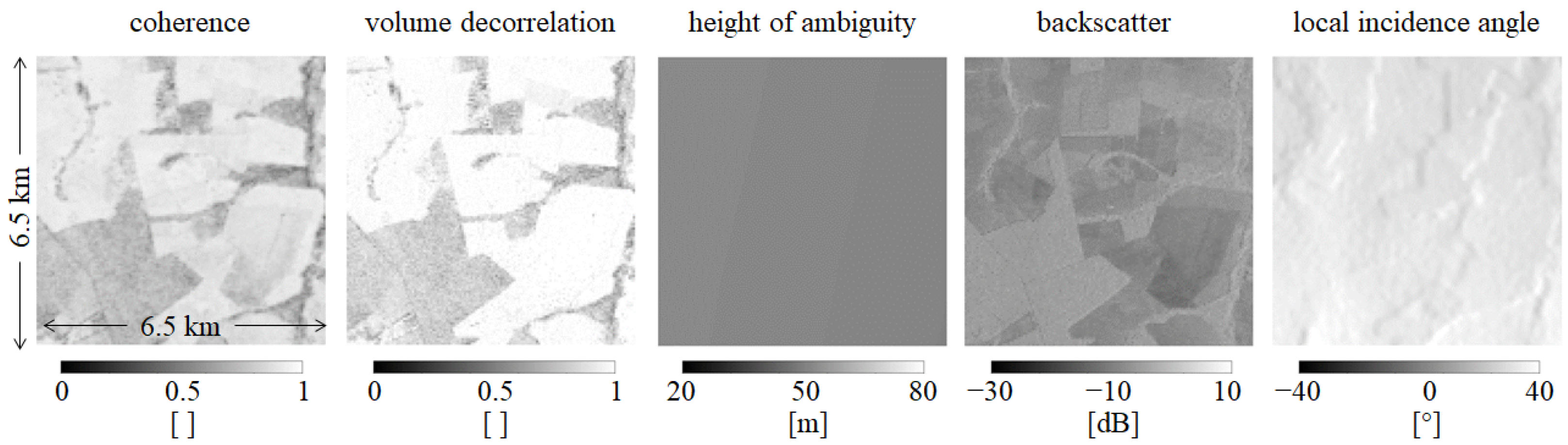
2.1. The TanDEM-X Interferometric Data Set and Its Properties

TanDEM-X is the first operational bistatic spaceborne SAR system comprising two spacecrafts, TerraSAR-X (TSX) and TanDEM-X (TDX), which act as a large single-pass radar interferometer with variable acquisition geometries [13]. Since the beginning of the mission in 2010, more than half a million high-resolution interferometric scenes have been acquired and processed for the generation of the global TanDEM-X digital elevation model (DEM), covering at least twice the complete Earth’s landmasses [14,15]. A single bistatic stripmap scene typically extends over an area of about 30 km in range by 50 km in azimuth, with a resolution of 12 m × 12 m for interferometric products. From this, the quicklook images of several SAR and InSAR quantities, such as backscatter and coherence maps, are generated as by-products at a ground resolution of 50 m × 50 m by applying a spatial multi-looking process. The global TanDEM-X quicklook data set has been exploited during the whole mission for performance monitoring activities as well as for the planning and optimization of new acquisitions [27]. Moreover, the limited computational load and the significant reduction in data volume, memory usage and processing time offered by the TanDEM-X quicklook data set allow for its fast exploitation with the aim of generating global geo-products, such as the TanDEM-X FNF map [12] and the TanDEM-X water body layer (WBL) [28].

The quality of the acquired TanDEM-X bistatic interferograms can be assessed by means of the interferometric coherence ${\gamma }_{{}_{\mathrm{Tot}}}$, which is defined as the normalized cross-correlation coefficient between the interferometric image pair [29,30]:

$${\gamma }_{{}_{\mathrm{Tot}}}=\frac{\left|E\right[u_1·u_2^{\ast }\left]\right|}{\sqrt{E\left[\right|u_1{|}^2]·E[|u_2{|}^2]}},$$

(1)

where $E[·]$ represents the statistical expectation, * the complex conjugate operator and $|·|$ the absolute value. $u_1$ and $u_2$ identify the master and slave images, respectively. ${\gamma }_{{}_{\mathrm{Tot}}}$ varies between 0 and 1 and it is typically estimated from real SAR data by applying a sliding boxcar window of W pixels centred around the considered pixel [31].

The total coherence can be factorized as presented in [32] and extended in [13], leading to:

$${\gamma }_{\mathrm{Tot}}={\gamma }_{\mathrm{Amb}}·{\gamma }_{\mathrm{Rg}}·{\gamma }_{\mathrm{Az}}·{\gamma }_{\mathrm{Temp}}·{\gamma }_{\mathrm{Quant}}·{\gamma }_{\mathrm{SNR}}·{\gamma }_{\mathrm{Vol}},$$

(2)

where the terms on the right-hand side are called decorrelation factors and account for different error contributions: SAR ambiguities (${\gamma }_{\mathrm{Amb}}$), coregistration errors in range and baseline decorrelation (${\gamma }_{\mathrm{Rg}}$), misregistration in azimuth and relative shift of the Doppler spectra (${\gamma }_{\mathrm{Az}}$), temporal decorrelation (${\gamma }_{\mathrm{Temp}}$), quantization (${\gamma }_{\mathrm{Quant}}$), thermal noise (${\gamma }_{\mathrm{SNR}}$) and volume decorrelation (${\gamma }_{\mathrm{Vol}}$). The first three terms (${\gamma }_{\mathrm{Amb}}$, ${\gamma }_{\mathrm{Rg}}$ and ${\gamma }_{\mathrm{Az}}$) are related to the specific sensor parameters and acquisition geometry [33], while ${\gamma }_{\mathrm{Temp}}$, ${\gamma }_{\mathrm{Quant}}$, ${\gamma }_{\mathrm{SNR}}$ and ${\gamma }_{\mathrm{Vol}}$ show a dependency on the specific illuminated scene on the ground and, consequently, on the kind of on-going backscattering mechanism. Given the bistatic nature of TanDEM-X, the coherence is not affected by temporal decorrelation, so ${\gamma }_{\mathrm{Temp}}=1$. Differently, volume decorrelation (${\gamma }_{\mathrm{Vol}}$) occurs when volumetric targets, such as vegetated areas or snow-covered regions, are illuminated and recorded by two slightly different positions, as in the case of single-pass across-track interferometry. ${\gamma }_{\mathrm{Vol}}$ can be derived by inverting (2) and compensating for all other decorrelation factors, as presented in [18].

In addition to the target’s properties, the volume decorrelation factor is closely related to the acquisition geometry [17]. Specifically, it is linked to the height of ambiguity, $h_{\mathrm{Amb}}$, which represents the topographic height difference of a complete $2\pi$ cycle of the interferometric phase [17]. For the bistatic case, $h_{\mathrm{Amb}}$ is defined as:

$$h_{\mathrm{Amb}}=\frac{\lambda ·R·\sin \left({\theta }_i\right)}{B_{\perp }},$$

(3)

where $\lambda$ is the radar wavelength, R the slant range, ${\theta }_i$ the acquisition incidence angle and $B_{\perp }$ the normal baseline (perpendicular to the line of sight). Moreover, it has been demonstrated that the decorrelation generated by volume scattering in densely vegetated areas can be related to vegetation parameters such as tree height and extinction rate [17].

The strong impact of the acquisition geometry on the volume decorrelation factor (and consequently on the total interferometric coherence) needs to be carefully taken into account when utilizing such a quantity as an input feature for the detection of forested areas from TanDEM-X InSAR data, which are acquired with a large variety of imaging geometries. In this context, the height of ambiguity represents one of the key parameters for the design of an effective training strategy for the proposed CNN.

Figure 1 depicts the height of ambiguity for TanDEM-X data-takes acquired over the Amazon rainforest from the end of 2010 to the end of 2016. The values span from a few meters to 200 m. The continuous variability of the physical baseline between the TerraSAR-X and TanDEM-X satellites is made possible by the adjustable, unique Helix close orbit formation [14]. Most values of $h_{\mathrm{Amb}}$ are comprised between 40 m and 60 m during the first TanDEM-X global coverage for the generation of the TanDEM-X digital elevation model (DEM) [15], from the end of 2010 to March 2012. The second TanDEM-X global coverage, from April 2012 to March 2013, was acquired with a lower $h_{\mathrm{Amb}}$ set around 35 m, aiming at improving the final DEM performance after a proper mosaicking of both global coverages [13,34]. During 2013 and 2014, further data-takes over the Amazon rainforest were acquired, but with typical $h_{\mathrm{Amb}}$ values higher than 80 m to limit the amount of volume decorrelation over vegetated areas. Very few acquisitions were acquired during the TanDEM-X science phase in 2014–2015 [34] and they were characterized by extremely low heights of ambiguity, which made the data extremely noisy. By the end of 2015 and during 2016, several images were acquired with different acquisition geometries and within a range of heights of ambiguity spanning between 20 m and 120 m.

Different considerations have to be formulated regarding the behaviour of water surfaces and their similarities with forests in InSAR data. Here, an almost completely specular reflection of the radar wave happens in presence of calm water, which leads to recorded backscatter values close to the system noise floor and to a complete decorrelation of the interferometric signal. Differently, in the presence of strong winds, surface waves typically increase the surface roughness of water as well, causing a significantly higher backscattered signal, while the InSAR coherence normally remains close to the lower bias (some low-level InSAR coherence has been measured in the presence of long waves, which typically do not concern inland rivers). Therefore, the use of the InSAR coherence in addition to backscatter for water detection increases the robustness of the classification, by reducing possible misclassifications caused by higher backscatter values in the presence of wind. Finally, by considering bistatic interferometry, it is quite unlikely that forests will completely decorrelate (reaching the lower bias) even for small heights of ambiguity. This aspect is crucial for a correct discrimination between forest and water classes.

2.2. External Reference Data

The complete set of external reference maps, used for the supervised training of the proposed U-Net as well as for the intercomparison between large-scale forest maps, is listed below:

• Landsat Tree Cover Map ([7,35]): This map is based on Landsat data acquired from 2000 to 2015. It is provided at a resolution of 30 m × 30 m and represents the percentage of forest covering the area defined by a 30 m pixel. Forest is defined as woody vegetation higher than 5 m. The tree cover map of 2010 has been used for training the U-Net on forest mapping.
• FROM-GLC Map ([8]): The FROM-GLC map has been used for the large-scale intercomparison of the generated mosaics. This land cover map has been generated at a pixel spacing of 10 m using a machine learning random forests classifier, trained on Landsat data acquired up to 2015, which has been updated to 2017 using additional multi-spectral data from the ESA Sentinel-2 mission.
• Palsar FNF Map ([10]): The PALSAR forest/non-forest map has been used for large-scale maps intercomparison. It is based on data acquired at the L band by the Japanese ALOS satellite series. The global PALSAR FNF map has been produced by thresholding the detected backscatter images acquired in cross polarization (HV channel) and it is provided with a 25 m pixel spacing. This map is available for 2010 and it is yearly updated starting from 2015.
• Sentinel-2 and Landsat Data: For validation purposes, we also utilized some specific multi-spectral Sentinel-2 and Landsat acquisitions over the Amazon rainforest.

Finally, it is worth pointing out that, before usage, all used external reference data were interpolated to the corresponding pixel size and output grid of the considered TanDEM-X input products (i.e., at a pixel spacing of 50 m), which were sampled on a uniform grid in latitude/longitude, referred to as the WGS84 Ellipsoid.

3. Baseline Classification Approaches

In this section, we briefly recall the baseline approaches already published in the literature for global forest and water mapping with TanDEM-X bistatic data that will be used as state-of-the-art algorithms for performance comparison with respect to the newly proposed CNN model.

3.1. Global Forest Mapping with TanDEM-X

Based on the findings of the work presented in [17], the volume decorrelation factor ${\gamma }_{{}_{\mathrm{Vol}}}$ was selected as the main input feature for the generation of the TanDEM-X forest/non-forest (FNF) map. The developed algorithm was based on a geometry-dependent fuzzy clustering classification approach [12], where the cluster centroids of both forest and non-forest partitions were defined a priori by first dividing the complete span of available heights of ambiguity into a set of sub-intervals. Then, for each sub-interval, the ${\gamma }_{{}_{\mathrm{Vol}}}$ mean value was evaluated for each class distribution, considering a dedicated training set of TanDEM-X images and a Landsat-based external reference for the correct grouping of both classes. It is worth mentioning that only acquisitions with $h_{\mathrm{Amb}}<100$ m were considered for the generation of the global TanDEM-X FNF map. On images acquired with higher $h_{\mathrm{Amb}}$ values, the forest classification was not performing well due to the acquisition geometry, characterized by smaller perpendicular baselines between the master and slave satellites, which reduce the sensitivity of ${\gamma }_{{}_{\mathrm{Vol}}}$ to vegetated areas. Afterwards, the procedure was repeated for three different ranges of incidence angles, namely characterizing the near, mid and far ranges of the operational TanDEM-X single-polarization (HH) stripmap beams constellation.

Given the variability of the interferometric coherence at the X band when considering different types of forest (mainly caused by changes in forest structure, density and tree height), three different sets of cluster centroids were derived for the generation of the global product, depending on the specific type of forest: tropical, temperate and boreal forests. Specifically, the Landsat reference data sets for the generation of the cluster centroids were located over the Amazonas, central Europe and Sweden, respectively. At the inference stage, a different set of centroids, selected depending on the acquisition latitudes, was utilized for classifying the input TanDEM-X images through the fuzzy clustering algorithm. Finally, the classified images were mosaicked in a single forest map following a weighted mosaicking process, which was necessary to achieve satisfactory accuracy for the output product [12].

For the generation of the global FNF map product, the entire data set of TanDEM-X acquisitions up to 2015 was considered. In particular, a quicklook version of the full-resolution images at 50 m × 50 m independent pixel spacing was used. Such images were obtained by the spatial multi-looking of the full-resolution TanDEM-X products at 12 m.

3.2. Global Watershed-Based Water Mapping with TanDEM-X

The coherence is a reliable indicator of the presence of water on the ground, since water surfaces typically appear as completely decorrelated areas. Therefore, for the generation of the global TanDEM-X water body layer (WBL), the authors relied on the coherence as the sole input feature for performing the classification and developed a detection method based on the watershed segmentation algorithm [28]. To do so, a Scharr transformation was firstly applied to the spatial gradient of the coherence in order to highlight its edges [36] and, secondly, the watershed algorithm was applied to the edges’ image for performing the actual segmentation [37]. Regions affected by geometric distortions, which typically lead to a complete decorrelation and may cause the erroneous detection of water surfaces, were filtered out by properly deriving shadow and layover maps from the acquisition geometry and the underlying topography. Overlapping classified images were then mosaicked together by computing a weighted average, where quality weights were assigned depending on the reliability of the water detection. For the generation of the global product, the same input data set used for the generation of the TanDEM-X FNF map was considered [28].

4. Methods

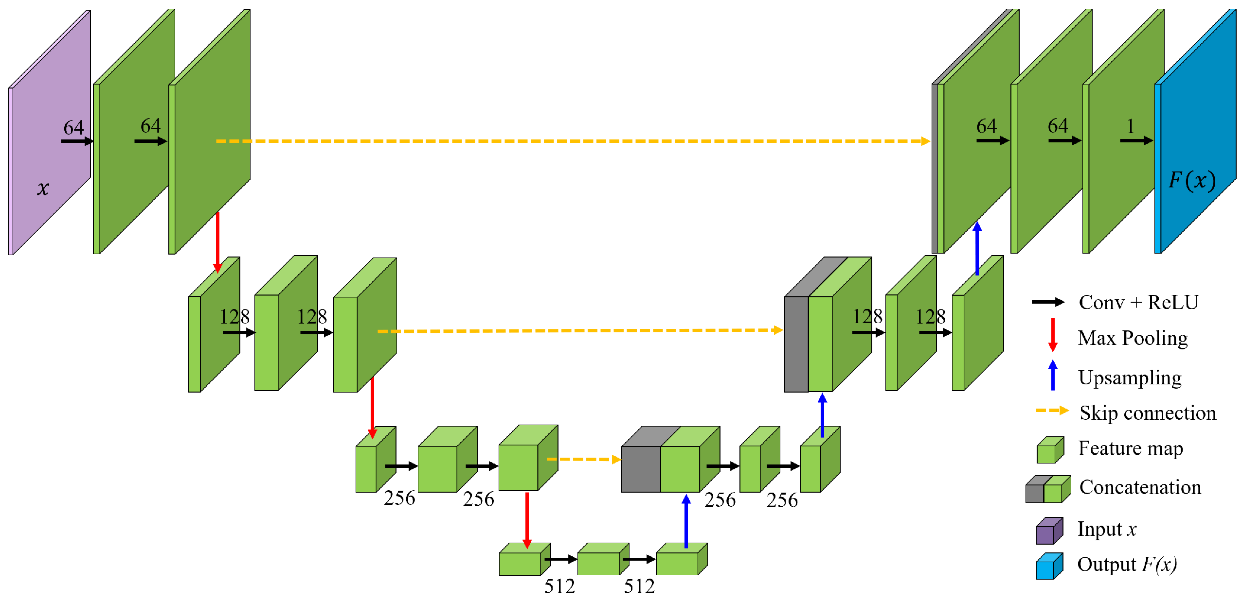
4.1. Proposed U-Net-like Architecture

By relying of the findings of the work presented in [23], we decided to keep the U-Net paradigm for the extension of forest mapping with TanDEM-X to a larger data set. In particular, the structure of the utilized U-Net-like architecture is presented in Figure 2. The encoder branch, on the left-hand side of the network, was then followed by a decoder one on the right-hand side, resulting in a U-like structure where each stage worked at a different resolution and abstraction level. Each stage of the encoder path consisted of a repeated application of two 3 × 3 convolution kernels, interleaved by rectified linear unit (ReLU) activations, with a terminal 3 × 3 convolutional layer with max pooling for the downsampling operation. Moreover, batch normalization was applied to speed up the network training and mitigate its dependence on the initialization [38]. The decoder section comprised mirrored stages with respect to the encoder one, which allowed for the progressive restoration of the retrieved feature’s spatial resolution, simultaneously reducing its number, by halving it at each 2 × 2 upscaling (performed through up-convolutions). The upsampled features were concatenated with the corresponding scale features coming from the encoding path through direct skip connections, which allowed for the direct propagation of high-resolution information from the encoder to the decoder. Such concatenated feature blocks were then convolved twice using again ReLU activation functions, as for the encoding path. The exit decoding stage comprised two additional convolutional layers. The last layer was a 1 × 1 convolution, which compacted the output feature map. This was followed by a sigmoid activation function, which finally provided the desired binary classification map by applying a threshold at 0.5. The number of convolutional kernels at each stage is reported in Figure 2, close to the corresponding operation symbol.

We fed the network using the following set of input feature maps: the SAR backscatter (in the form of radar brightness ${\beta }^0$), the interferometric coherence ${\gamma }_{\mathrm{Tot}}$, the volume decorrelation factor ${\gamma }_{\mathrm{Vol}}$, the local incidence angle ${\theta }_i$ and the height of ambiguity $h_{\mathrm{Amb}}$. An example of input feature patches is presented in Figure 3. The choice of this set of input features was based on the conclusions derived from the work presented in [23], where the impact of the different TanDEM-X features on forest detection using U-Net was firstly investigated. With respect to the work in [23], $h_{\mathrm{Amb}}$ was added, as the key descriptor accounting for the variability of TanDEM-X acquisition geometries. As for the generation of the TanDEM-X FNF map, we decided to work with input features at 50 m resolution, in order to limit the computational load.

4.2. Generation of the Training Data Set

For training the U-Net architecture, we developed an ad hoc strategy aimed at generalizing the model with respect to all possible acquisition geometries of the TanDEM-X data set. In order to simplify the problem of generating well-balanced training data sets, we selected two different sets of images over the Amazon rainforest, characterized by different peculiarities, to train two separate U-Net-like architectures for forest and water mapping, respectively. The resulting output binary layers were then combined in a final classification map providing three classes: forest, non-forest and water.

Forest Mapping Task: We utilized as an external reference the Landsat Tree Cover map recalled in Section 2.2: we set an empirical threshold at 50% on the tree cover density map to generate a reference binary forest/non-forest map for training and validation purposes. In order to account for the different acquisition geometries, we first divided the acquisition incidence angles ${\theta }_{\mathrm{i}}$ into three main ranges: (a) ${\theta }_{\mathrm{i}}<{35}^{\circ }$, (b) ${\theta }_{\mathrm{i}}\in [{35}^{\circ },{45}^{\circ }]$ and (c) ${\theta }_{\mathrm{i}}>{45}^{\circ }$. Similarly, we divided the overall span of $h_{\mathrm{Amb}}$, ranging from 20 m to about 120 m, into sub-intervals of 2 m. Where possible, we utilized up to 5 images per interval (regarding both $h_{\mathrm{Amb}}$ and ${\theta }_{\mathrm{i}}$). The overall distribution of the input acquisitions with respect to $h_{\mathrm{Amb}}$ and ${\theta }_{\mathrm{i}}$ is depicted in Figure 4. As it can be seen, $h_{\mathrm{Amb}}$ ranges between 30 m and 120 m are well sampled with all three incidence angles’ intervals, while mid- and far-range incidence angles are not available at $h_{\mathrm{Amb}}<30$ m. Nevertheless, it is worth pointing out that the vast majority of operational TanDEM-X acquisitions were acquired with $h_{\mathrm{Amb}}>30$ m. Moreover, we selected only images with a forest content comprised between $30\%$ and $70\%$, in order to mitigate class imbalance. The number of pixels flagged as forest, with respect to the total number of valid pixels in each image, was derived from the reference data. Overall, we considered 455 input TanDEM-X acquisitions over the Amazon rainforest, from which we extracted patches of size 128 × 128 pixels, resulting in more than one million patches. All data-takes were acquired between 2011 and 2012, in order to assure the best possible temporal agreement with the considered reference map of 2010.

Water Mapping Task: To train the U-Net-like CNN for water detection, we changed the data set generation strategy, since the decorrelation on water surfaces is almost independent of the acquisition geometry. In this case, the bottleneck is given by the lower amount of available water samples, given the limited extension of water surfaces, with respect to the surrounding land cover classes. For this purpose, we utilized a different set of 376 TanDEM-X images over the Amazon rainforest region, characterized by a mean water content of at least 35% according to the reference data and representative of different types of water bodies, such as open water, lakes and rivers.

4.3. Training Process

The network was trained from scratch to avoid any type of transfer learning, taking advantage of the increased amount of available data with respect to previous studies. We optimized the network by employing the Adam algorithm [39], with the initial learning rate set to ${10}^{-4}$. We used minibatches comprising 32 patches, randomly sampled from the overall training validation data set (80% reserved for training and 20% for validation). As a loss function, we utilized a combination of the cross-entropy loss, which showed nice convergence properties, and the Jaccard similarity loss, which accounted for the spatial distribution of neighbouring pixels belonging to the same class, as performed in [23]. Figure 5 depicts the loss function and the accuracy trends for the training and validation sub-sets, considering 50 epochs. If, on the one hand, a good convergence between the training and validation loss functions is observed, on the other hand, a slightly better performance of the validation loss is visible during the first epochs. This behaviour is probably due to the fact that, working with minibatches, the training loss is calculated for each backpropagation step during an epoch, while the validation loss is calculated at the end of each epoch only. Since each backpropagation step within a single epoch could improve the model significantly, especially during the first few epochs when the network weights are still relatively untrained, it is not uncommon to obtain a lower validation loss which later on converges to the training one.

4.4. Performance Assessment Metrics

We assess the quality of the produced TanDEM-X classification maps by computing the standard confusion matrices, with respect to external reference maps, and evaluating several performance metrics. For each land cover class, the four terms in the confusion matrix were defined as: true positives ($TP$)-pixels classified with the same land cover (forest/water) in both maps; false positive ($FP$)-pixels wrongly assigned in the TanDEM-X classification map to one of the two classes (forest/water) and belonging in the reference map to the non-forest/non-water class; false negative ($FN$)-pixels classified in the TanDEM-X image as non-forest/non-water and assigned to one of the land covers (forest/water) in the reference map and true negative ($TN$)-pixels classified as non-forest/non-water in both maps.

For the final performance evaluation, we considered the overall accuracy ($OA$) and the F-score, which can be derived from the confusion matrices and are defined as follows [40]:

• The overall accuracy ($OA$) represents the overall correctly classified pixels, with respect to the total number of classified pixels, considering all land cover classes, and is defined as:

  $$OA=\frac{TP+TN}{TP+TN+FP+FN}$$

  (4)
• The F-score, also called the $F1$-score, is an accuracy metric that ranges between 0 and 1 and is expressed as:

  $$F-\mathrm{score}=\frac{2\times TP}{2\times TP+FP+FN}$$

  (5)

The F-score is mainly used to evaluate binary classifications and is useful especially when dealing with imbalanced data sets. Moreover, in this work the F-score was evaluated for each single land cover class, separately. On the other hand, the $OA$ has the advantage of being easily interpretable but the disadvantage that it is not very robust when the data are unevenly distributed.

Moreover, we also validated our proposed approach by comparing the TanDEM-X mosaic over the Amazon rainforest, generated using acquisitions performed in 2016, and a forest/non-forest map derived from Sentinel-2 optical images acquired during the dry season between June and August 2016. For the derivation of the Sentinel-2 FNF map, we relied on the normalized difference vegetation index (NDVI) and the normalized difference moisture index (NDMI) [41]. Both indexes are good indicators of the presence of vegetation in Sentinel-2 images and are obtained from a combination of the Sentinel-2 spectral bands 4, 8 and 11 [42]. In order to properly derive a binary layer we applied thresholds of 0.7 and 0.25 on the NDVI and NDMI, respectively, where the threshold values were computed to optimally separate the distributions of forest and non-forest classes within the corresponding bimodal histograms, shown later on in Figure 10.

5. Results

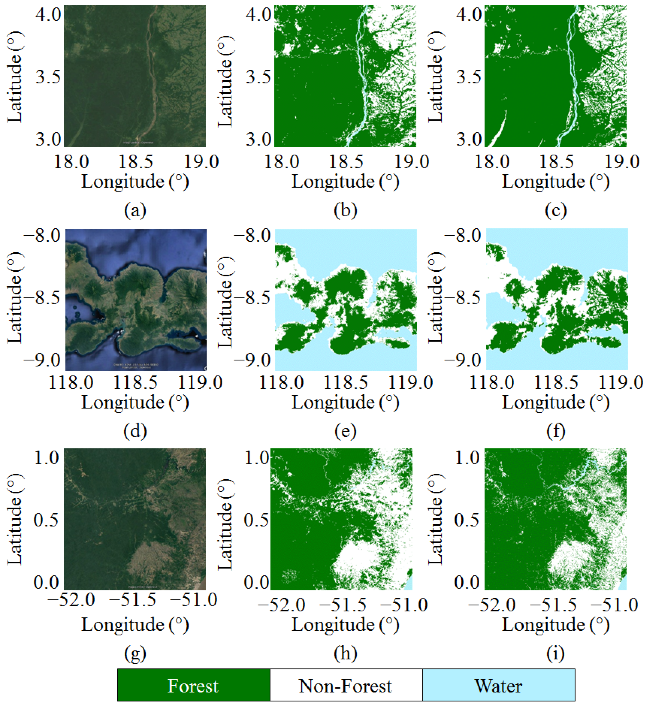
5.1. Single-Scene Classification

After training the U-Net-like CNN over the Amazon rainforest as presented in Section 4.2, a further 976 TanDEM-X quicklook images with at least 10% forest content over the Amazon rainforest and representative for all the considered ranges of $h_{\mathrm{Amb}}$ values and incidence angles were considered for testing its performance. Clearly, the test data set was not used during the training phase.

Figure 6 shows two examples of single-scene classification by considering (top) $h_{\mathrm{Amb}}=32$ m and (bottom) $h_{\mathrm{Amb}}=99$ m. From left to right, each row depicts the Landsat reference map, together with the classification maps obtained by applying the baseline clustering approach (CL-FNF map) and the proposed deep-learning-based approach (CNN-FNF map), respectively. The detected forest is shown in green, the non-forested areas are depicted in white and the water is represented in cyan. The CNN-based approach is more robust to noise with respect to the baseline clustering and therefore able to correctly close gaps over forested areas as well as to better detect clear cuts. Additionally, topographic effects are also mitigated due to the utilization of the local incidence angle as an input feature. The improvement in the classification accuracy obtained through the CNN is clearly visible, in particular when considering high $h_{\mathrm{Amb}}$ values, which are typically characterized by limited volume decorrelation and, consequently, by higher classification uncertainty between forest and non-forest pixels. This is confirmed when considering the F-score, computed with respect to the Landsat reference image. Indeed, for the first image with $h_{\mathrm{Amb}}=32$ m, in the case of the CL-FNF map we obtained F-scores of 0.83 and 0.86 for the non-forest and forest classes, respectively, while, when considering the CNN-FNF map, the F-score achieved 0.96 for both classes (water surfaces were not present). Regarding the second image, characterized by $h_{\mathrm{Amb}}=99$ m, the F-scores of the CL-FNF map reached 0.5, 0.85 and 0.81 for the non-forest, forest and water classes, respectively, while the F-scores of the CNN-FNF map increased by more than 10% for all three classes, achieving 0.88, 0.98 and 0.92, respectively.

A more exhaustive performance comparison between the proposed approach and the baseline CL approach is presented in Figure 7, where all test images are considered. Figure 7a depicts the difference in F-score between the two methods. The parameter was evaluated with respect to the forest class. An increase was F-score was obtained for the vast majority of the images (positive values), indicating a significant performance improvement. Indeed, the mean F-score, computed over all the available acquisitions, was equal to 0.88 for the CNN-FNF map, while it reduced to 0.75 for the CL-FNF map case. Moreover, the effectiveness of the training strategy can be seen in Figure 7b, which depicts the performance obtained by comparing the forest classification for both considered approaches as a function of the percentage of forest in the image, according to the Landsat forest map used as a reference. An improvement in the detection of forest with the CNN-FNF map is overall observable but especially noticeable over densely forested areas (the percentage of forest samples > 80%). Differently, Figure 7c shows the performance obtained by comparing the forest classification as a function of the $h_{\mathrm{Amb}}$. To perform this last analysis, we considered a long time-series of TanDEM-X images acquired over the same area with varying acquisition geometry. The improvement in the classification of forest with the CNN-FNF map is clearly visible, especially for values of $h_{\mathrm{Amb}}>90$ m, where the performance of the clustering approach appears to be strongly degraded. According to that, with the proposed method, single images acquired with higher $h_{\mathrm{Amb}}$ can provide reliable detection of forested areas.

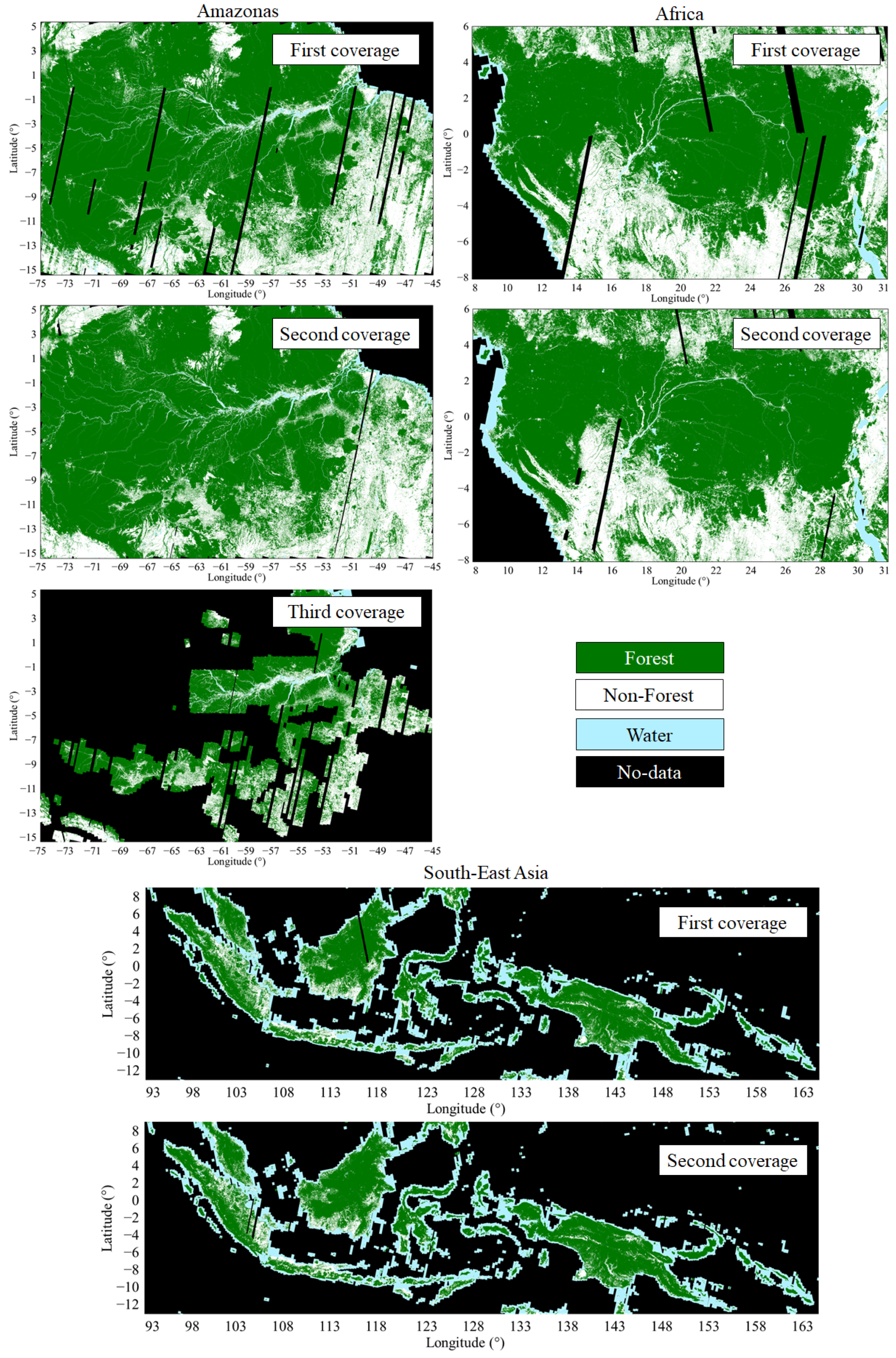
5.2. Large-Scale Mosaics

Overall, we classified more than 20,000 TanDEM-X images acquired over tropical forests between the end of 2010 and the beginning of 2017 using the proposed methodology. We considered acquisitions from three separate coverages of the whole area, spanning over three different continents, which were designed during different phases of the TanDEM-X mission. In particular, two almost complete coverages were performed during the first and second years of operation (i.e., 2011 and 2012–2013, respectively), during which data for the generation of the global TanDEM-X digital elevation model were acquired [15]. A third partial coverage was performed later on in 2016 over the Amazon forest only [14]. The reliable performance achieved for all different acquisition geometries over the Amazon rainforest allows for the generation of large-scale time-tagged mosaics, skipping the weighted mosaicking process of overlapping acquisitions as performed for the generation of the global TanDEM-X forest/non-forest map to achieve a sufficient accuracy [12]. Moreover, the use of external reference maps to filter out water surfaces, as performed for the global FNF product, is not necessary anymore with the proposed methodology.

The U-Net-like CNN, trained over the Amazon rainforest only, was used both for classifying the entire Amazon basin and for extending the classification over the other tropical areas in central Africa and South-East Asia as well. The aim of this last activity was to test the generalization capability of the network and to investigate a potential performance degradation, caused by changes in the characteristics of the illuminated forests.

Figure 8 shows the three large-scale mosaics, obtained from the different TanDEM-X coverages for the three different macro-regions of interest. A detail of the classification map over the Brazilian state of Rondônia, generated using input images acquired during the first TanDEM-X global coverage only (2011), is presented in Figure 9. For visual comparison purposes, an optical image acquired by Landsat over the same area is depicted as well.

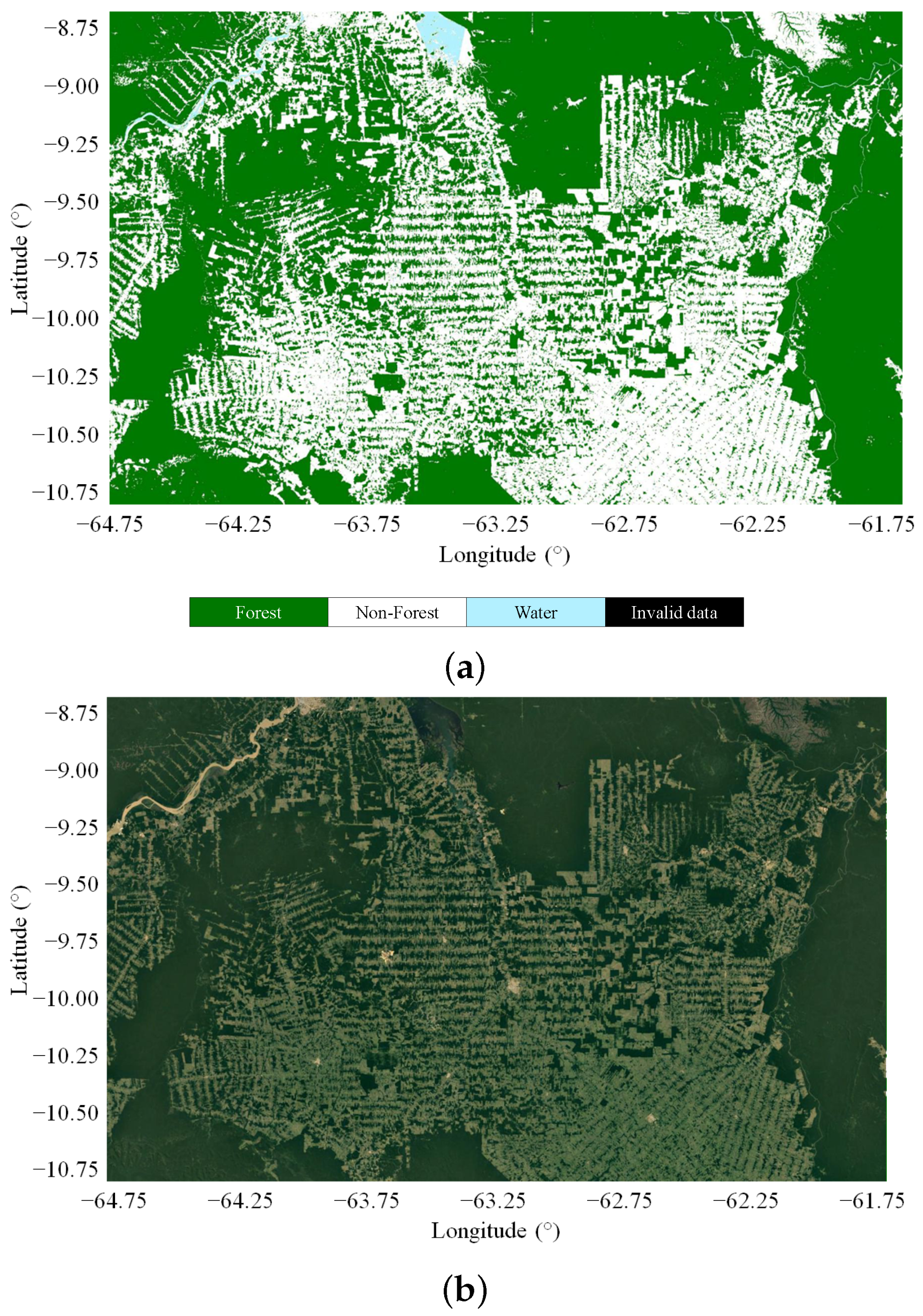
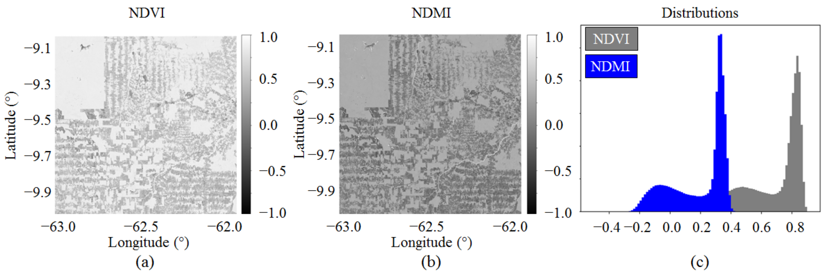
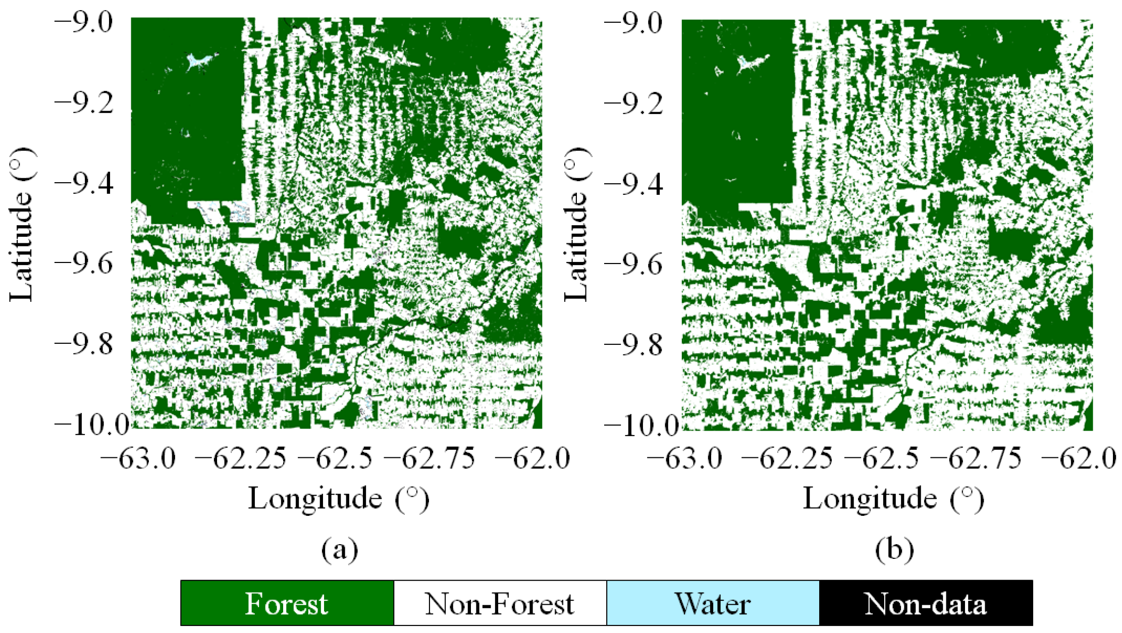
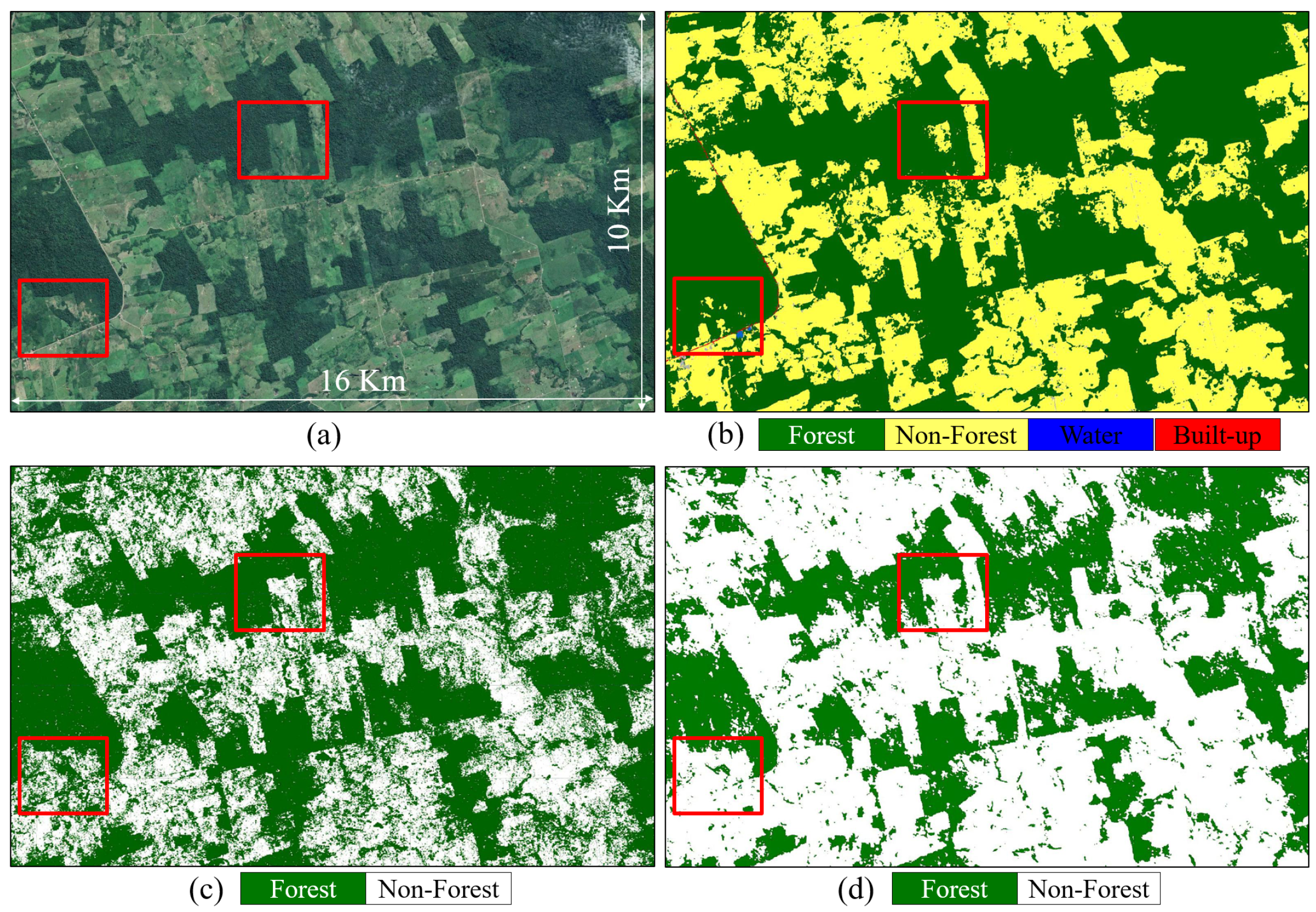
5.3. Local Validation with Sentinel-2 Data

In Figure 10, we show the Sentinel-2 NDVI and NDMI and the corresponding histograms for a Sentinel-2 acquisition over the Amazon rainforest in the state of Rondônia. As it can be seen from the histograms, both indexes show a bimodal behaviour, which characterizes the presence of two main land cover classes: forest and non-forest. By thresholding the NDVI at 0.7 and the NDMI at 0.25 and combining both outputs, we generated a binary FNF map, which can be used for validation, as proposed in [43]. On the other hand, for the detection of water surfaces, we relied on the WorldCover 2020 land cover product [9].

A total of 96 TanDEM-X geocells, with at least 30% valid samples after clouds and cloud-shadow removal on Sentinel-2 images, were considered for the validation. The generated Sentinel-2 maps were re-projected and brought to the same coordinate reference system, geographic extent and spatial resolution as the considered TanDEM-X FNF maps. The complete performance accuracy obtained for the validation of the TanDEM-X mosaic is detailed in

Table 1. Performance comparison between TanDEM-X mosaic over the Amazonas rainforest of 2016 and Sentinel-2 (S2). The $OA$ is presented for each mosaic. The number of evaluated geocells is specified in brackets. The F-score is shown for the three land cover classes: non-forest, water and forest. For each case, only geocells with a certain amount of samples belonging to each land cover class (>1%, >5% and >10%) have been considered. The overall amount of pixels belonging to each class has been estimated from the external map used in the comparison.

			F-Score
2016	Samples	OA	Non-Forest	Water	Forest
S. America	>1%		66.87 (93)	74.30 (47)	84.29 (95)
	>5%	84.40 (96)	71.03 (83)	85.09 (24)	85.08 (94)
	>10%		73.33 (75)	87.80 (15)	86.43 (92)

. The overall accuracy ($OA$) was higher than 84%, and the F-score for the forest class showed a high agreement for all considered geocells as well. In addition, for the water class, a good performance was measured for geocells with a water content higher than $5\%$. For geocells with a water content lower than $5\%$, generally characterized by the presence of narrow rivers, the input resolution of the TanDEM-X quicklook products seems not sufficient to properly detect such small water bodies. For the non-forest class, a lower performance was obtained. Temporal changes, caused especially by deforestation activities, accounted for an additional performance reduction. Indeed, the TanDEM-X FNF mosaic was generated with images acquired during 2016 and the beginning of 2017, while the Sentinel-2 FNF maps were obtained from images acquired during a limited period of three months only (June–August 2016), when it was possible to acquire images with a cloud cover percentage lower than $20\%$. In addition, the different sensitivities of the TanDEM-X and Sentinel-2 sensors to vegetation close to rivers slightly impacted the overall performance of the non-forest class.

Finally, for visual inspection purposes, Figure 11 shows an example of the TanDEM-X and Sentinel-2 FNF maps for the geocell previously considered in Figure 10, and a good agreement between both maps can be appreciated.

5.4. Intercomparison with Global Products

For the generated TanDEM-X large-scale mosaics, we performed an intercomparison with similar available products, generated from remotely sensed spaceborne data. All utilized external land cover reference data sets were interpolated to the same grid and spatial resolution as those of the considered TanDEM-X classification maps. Since different time-tagged mosaics over the tropical areas have been produced with TanDEM-X data, we utilized external reference maps, where available, whose input data were approximately acquired during similar time-spans as the TanDEM-X data, in order to reduce inconsistencies caused by possible temporal changes between the two maps. To do so, we compared the TanDEM-X mosaics with data mainly acquired during 2011 and the beginning of 2012 with the PALSAR forest/non-forest map of 2010 [10] and the TanDEM-X mosaics with data acquired in 2012 and during the whole of 2013 with two maps referred to in 2015: the PALSAR forest/non-forest map of 2015 and the FROM-GLC [44]. Finally, the mosaic over the Amazonas generated from TanDEM-X acquisitions between 2016 and 2017 was compared with two additional maps: the PALSAR forest/non-forest map of 2017 and the FROM-GLC (updated to 2017 with Sentinel-2 data) [8].

The complete performance accuracy of all the TanDEM-X mosaics is detailed in

Table 2. Performance comparison between TanDEM-X mosaics and PALSAR. For an explanation of each field, please refer to the caption of Table 1.

			F-Score
2011	Samples	OA	Non-Forest	Water	Forest
S. America	>1%		68.45 (432)	63.70 (230)	86.25 (582)
	>5%	89.72 (586)	77.06 (318)	76.87 (64)	87.05 (576)
	>10%		78.93 (281)	82.83 (31)	87.96 (567)
Africa	>1%		61.78 (234)	88.77 (66)	82.48 (301)
	>5%	85.81 (302)	71.11 (172)	95.99 (33)	82.70 (300)
	>10%		74.39 (148)	97.11 (26)	83.49 (296)
Asia	>1%		64.35 (516)	97.30 (583)	71.30 (500)
	>5%	86.20 (638)	66.73 (392)	98.41 (554)	77.47 (411)
	>10%		69.00 (311)	98.69 (537)	79.02 (358)
2013	Samples	$\mathit{OA}$	Non-Forest	Water	Forest
S. America	>1%		66.11 (467)	59.04 (251)	85.96 (580)
	>5%	89.79 (589)	76.03 (345)	55.49 (84)	88.04 (563)
	>10%		80.01 (288)	54.41 (44)	89.21 (551)
Africa	>1%		60.90 (221)	78.46 (88)	83.61 (301)
	>5%	86.06 (301)	71.49 (158)	90.34 (38)	83.62 (300)
	>10%		74.84 (133)	97.90 (29)	84.00 (297)
Asia	>1%		65.72 (515)	97.86 (576)	75.68 (511)
	>5%	88.38 (630)	68.91 (382)	98.93 (546)	80.09 (426)
	>10%		71.30 (293)	99.04 (531)	82.52 (370)
2016	Samples	$\mathit{OA}$	Non-Forest	Water	Forest
S. America	>1%		70.52 (258)	70.49 (92)	86.98 (290)
	>5%	88.06 (296)	76.18 (211)	79.57 (47)	87.25 (289)
	>10%		79.31 (180)	85.53 (25)	87.47 (288)

and

Table 3. Performance comparison between TanDEM-X mosaics and FROM-GLC. For an explanation of each field, please refer to the caption of Table 1.

			F-Score
2013	Samples	$\mathit{OA}$	Non-Forest	Water	Forest
S. America	>1%		67.63 (462)	74.17 (222)	86.60 (583)
	>5%	90.61 (589)	78.79 (332)	85.70 (60)	87.28 (577)
	>10%		81.27 (280)	88.04 (32)	88.50 (564)
Africa	>1%		62.86 (263)	86.31 (84)	78.98 (300)
	>5%	85.56 (303)	71.73 (206)	96.54 (36)	79.78 (295)
	>10%		74.34 (183)	98.64 (29)	81.03 (287)
Asia	>1%		66.16 (425)	95.68 (609)	81.05 (545)
	>5%	90.41 (634)	72.58 (284)	98.19 (567)	83.35 (469)
	>10%		73.63 (214)	98.81 (545)	84.66 (418)
2016	Samples	$\mathit{OA}$	Non-Forest	Water	Forest
S. America	>1%		69.88 (255)	61.34 (111)	87.11 (290)
	>5%	87.58 (296)	75.64 (206)	66.36 (56)	87.38 (289)
	>10%		77.77 (178)	78.77 (28)	87.59 (288)

. The overall accuracy ($OA$) was in all cases higher than 85%, and reaching 90% in some specific cases. In general, for the forest class a high agreement well over 80% is observed over all different tropical forest areas, pointing out the potential of the proposed method for forest mapping and land cover classification with TanDEM-X data. Major differences are observed between the PALSAR FNF maps and the TanDEM-X ones over South-East Asia, with a decrease in the overall performance. This is probably due to the strong topography which characterizes the area and affects the recorded SAR and InSAR features as well as to the dynamic changes caused by deforestation and land use. In addition, in central Africa a slightly different sensibility to vegetation between radar and optical sensors (TanDEM-X vs. FROM-GLC maps) reduces the overall performance of the forest class. With respect to the water class, the U-Net is able to detect water bodies with high precision, especially along coastal areas, as observed over South-East Asia, where an agreement between maps >95% is obtained. Over the other tropical areas, and especially over the Amazon rainforest, where many geocells have a water content <5%, the TanDEM-X water detection suffers from the not-sufficient resolution of the used input TanDEM-X quicklook images (50 m) for the detection of narrow rivers, generally reducing the performance of the generated maps.

Detailed examples of the intercomparison between the considered maps are presented in Figure 12. An optical image (acquired with Landsat and taken from Google Earth ©) is attached in each case for visual comparison purposes. Each area corresponds to a geocell extending by 1${}^{\circ }\times$1${}^{\circ }$ degrees in latitude/longitude. The comparison between TanDEM-X 2011 and PALSAR 2010 maps is made on a geocell over Central Africa on the northern border of the dense forest. Good agreement is observed for the forest (F-score of 0.95) and water (F-score of 0.84) classes. Major differences are observed for the non-forest class (F-score of 0.77). Here, deforestation (changes in time) and different sensitivities between the X and L band radar sensors to the forest close to the rivers accounts for a slightly lower performance for this land cover class. In the case of the geocell over South-East Asia, the coastal area is well caught by both compared maps: TanDEM-X 2013 and PALSAR 2015 (F-score of 0.99 for the water class). The forest (F-score of 0.84) and non-forest (F-score of 0.77) areas show a good agreement, too. Similarly, for the geocell over the Amazon rainforest, a good agreement for all classes is observed as well (F-score of 0.91 for forest, of 0.70 for water and of 0.78 for non-forest). The TanDEM-X CNN-FNF map is compared with the FROM-GLC one. The higher resolution of this last map accounts for the major differences: clear-cuts are mapped at a higher level of detail, being able to catch isolated trees. Differences in the status of the deforestation activities are observed, mainly caused by the time difference in the acquisition of the data.

In general, it is necessary to point out that the utilized reference maps are not error-free, which can of course further affect the resulting agreement. For example, the FROM-GLC map is based on optical data only. This represents a strong limitation, since we are considering regions mostly covered by clouds for a large part of the year, which lead to invalid or unreliable values. Moreover, when comparing maps acquired with different sensors, at different resolutions, and especially at different temporal intervals, a certain grade of disagreement can be expected, with forests, as well as water bodies, being a very dynamic ecosystem, typically characterized by frequent changes in time.

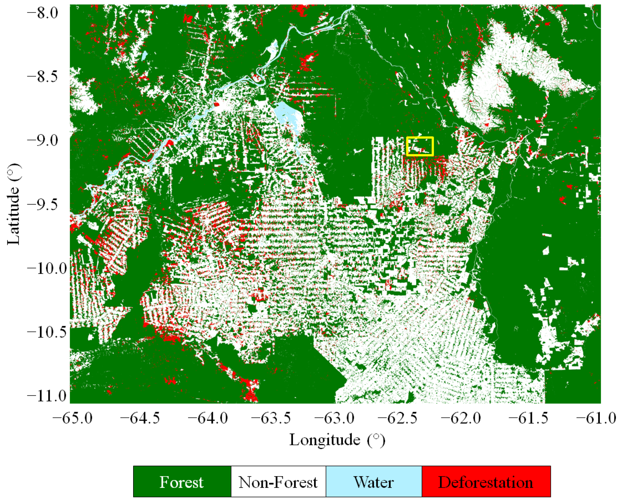
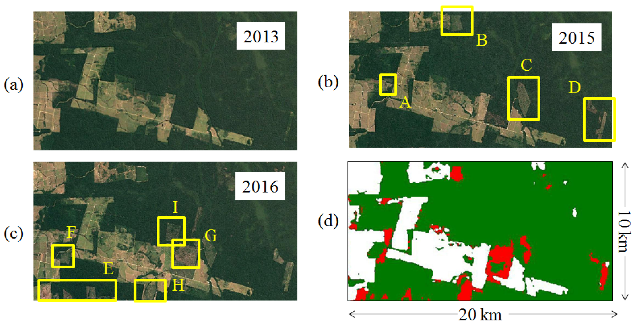
6. Potential for Change Detection and Deforestation Monitoring

The large-scale CNN-FNF maps produced from the different TanDEM-X coverages can be exploited for detecting changes and monitoring dynamic phenomena such as deforestation activities. Due to the high accuracy of the products, a reliable change detection can already be performed by simply differentiating consecutive maps. An example is presented in Figure 13, where an extended region in the Brazilian state of Rondônia is considered. Red areas correspond to deforested regions where trees were cut down between 2013 and 2016 (50,700 ha). Deforestation patterns are clearly visible, and single clear-cuts can be properly identified and associated with a specific time span.

In order to provide a more detailed example of the accuracy of the generated product, we concentrate on the small patch highlighted by the yellow square, which is separately analysed in Figure 14. Here, three Landsat optical images of the region, acquired at the end of 2013, 2015 and 2016, respectively, are depicted together with the corresponding change map derived by differentiating the TanDEM-X CNN-FNF maps of 2013 and 2016. For each single year, the yellow squares superimposed to the optical images identify new clear-cuts. As it can be seen, all main detected clear-cuts (from A to H) are correctly detected in the CNN-FNF map as well (deforested 1100 ha). Only the clear-cut I is not detected, which is probably due to the fact that vegetation was cut down after the acquisition of the TanDEM-X image (the Landsat image in (c) is from December 2016).

Clearly, the 50 m resolution of the considered TanDEM-X quicklook data limits the possibility to properly detect very small changes, such as single trees or narrow roads. This aspect will be considered in future works, by optimizing the proposed DL model for the original TanDEM-X coregistered L1B products at full resolution. A first hint on the potential of such an approach for high-resolution forest mapping can be seen in Figure 15. Here, we can perform a visual inspection of a small area located in the Brazilian Amazon forest, mapped at high resolution by different sensors. Figure 15a depicts the RGB optical image acquired by Landsat on 6 June 2018, Figure 15b shows the corresponding land cover map at 10 m resolution from the ESA WorldCover 2020 product [9] (which represents the land cover from 1 January to 31 December 2020 and is derived from Sentinel-1 and Sentinel-2 data), while Figure 15c,d correspond to TanDEM-X FNF maps at 12 m resolution obtained from a bistatic acquisition acquired on 28 May 2020, by applying the baseline clustering approach (c) and the proposed CNN (d), respectively. It is important to remark that both TanDEM-X approaches have not been specifically adapted to the high-resolution case, but simply applied as performed for the 50 m quicklook images. One can notice how the deforestation patterns are clearly recognizable in both TanDEM-X cases, even though the clustering approach provides a much noisier detection of clear-cuts. The CNN is already able to better resolve small gaps and to provide a more robust estimation. This behaviour was already observed at 50 m resolution. On the other hand, some small gaps appear in the detection of closed forest areas (e.g., in the top-right corner of image (d)), probably due to slightly different spatial patterns at high resolution that the network has not seen during training. Regarding this aspect, a fine tuning of the proposed U-Net with sample high-resolution data needs to be further investigated. Finally, some discrepancies between the ESA WorldCover 2020 and the TanDEM-X maps are highlighted by the red squares in Figure 15. Since all the input images utilized for the generation of the WorldCover 2020 and of the TanDEM-X FNF maps were acquired after the considered Landsat reference image, it appears that the WorldCover 2020 product tends to slightly overestimate forests with respect to TanDEM-X, suggesting different sensitivities of Sentinel-1/Sentinel-2 and TanDEM-X to the presence of vegetation. In addition, this aspect could be further investigated after fine-tuning the proposed CNN for high-resolution data.

7. Conclusions

In this paper, we presented an approach based on the use of deep convolutional neural networks for mapping forests and water surfaces at large-scale by utilizing TanDEM-X bistatic InSAR acquisitions. Starting from previously published research, we extended the model’s generalization capabilities by considering new input features, such as the height of ambiguity, and we developed an ad hoc training strategy for the network which takes into account the variability of TanDEM-X acquisitions at global scale with respect to the acquisition geometry. Due to this strategy, the proposed U-Net-based model is suitable for large-scale processing and more robust with respect to state-of-the-art approaches. Overall, the results over tropical forests show a good agreement with external reference maps and a significant accuracy improvement with respect to the baseline approach, based on a supervised clustering and previously used forest mapping with TanDEM-X data at global scale. Moreover, due to the unique ability of radar sensors to acquire data also in the presence of clouds, we are able to generate highly accurate, time-tagged and gap-free products. This could provide the scientific community with valuable data for assessing dynamic changes over forested regions, such as tropical or boreal forests, which are hidden by clouds for most of the year.

The trained CNN has been used to classify TanDEM-X images acquired over different tropical areas, spanning from the Amazon and African rainforests to South-East Asia. The improved classification accuracy allowed for the generation of time-tagged, large-scale mosaics, each of those referring to a specific phase of the TanDEM-X mission. This opens up new possibilities for effectively monitoring changes and deforestation phenomena in the considered areas. As a further investigation topic, we could rely on the training strategy presented in this work for re-training or fine-tuning the proposed model for high-resolution TanDEM-X data and different types of forests, such as temperate or boreal forests, with the aim to effectively detect selective logging patterns and forest degradation phenomena.

References

1. Silva-Junior, C.; Moreira Pessôa, A.C.; Carvalho, N.; dos Reis, J.A.; Anderson, L.; Aragão, L. The Brazilian Amazon deforestation rate in 2020 is the greatest of the decade. Nat. Ecol. Evol. 2021, 5, 144–145. [Google Scholar] [CrossRef]
2. Gao, Y.; Skutsch, M.; Paneque-Gálvez, J.; Ghilardi, A. Remote sensing of forest degradation: A review. Environ. Res. Lett. 2020, 15, 103001. [Google Scholar] [CrossRef]
3. Reiche, J.; Mullissa, A.; Slagter, B.; Gou, Y.; Tsendbazar, N.E.; Odongo-Braun, C.; Vollrath, A.; Weisse, M.J.; Stolle, F.; Pickens, A.; et al. Forest disturbance alerts for the Congo Basin using Sentinel-1. Environ. Res. Lett. 2021, 16, 024005. [Google Scholar] [CrossRef]
4. Hansen, M.C.; Defries, R.S.; Townshend, J.R.G.; Sohlberg, R. Global land cover classification at 1 km spatial resolution using a classification tree approach. Int. J. Remote Sens. 2000, 21, 1331–1364. [Google Scholar] [CrossRef]
5. Rast, M.; Bezy, J.L.; Bruzzi, S. The ESA Medium Resolution Imaging Spectrometer MERIS a review of the instrument and its mission. Int. J. Remote Sens. 1999, 20, 1681–1702. [Google Scholar] [CrossRef]
6. Pagano, T.; Durham, R. Moderate Resolution Imaging Spectroradiometer (MODIS). Proc. SPIE 1993. [Google Scholar] [CrossRef]
7. Hansen, M.C.; Potapov, P.V.; Moore, R.; Hancher, M.; Turubanova, S.A.; Tyukavina, A.; Thau, D.; Stehamn, S.V.; Goetz, S.J.; Loveland, T.R.; et al. High-resolution global maps of 21st century forest coverage change. Science 2013, 342, 850–853. [Google Scholar] [CrossRef]
8. Gong, P.; Liu, H.; Zhang, M.; Li, C.; Wang, J.; Huang, H.; Clinton, N.; Ji, L.; Li, W.; Bai, Y.; et al. Stable classification with limited sample: Transferring a 30-m resolution sample set collected in 2015 to mapping 10-m resolution global land cover in 2017. Sci. Bull. 2019, 64, 370–373. [Google Scholar] [CrossRef]
9. Zanaga, D.; Van De Kerchove, R.; De Keersmaecker, W.; Souverijns, N.; Brockmann, C.; Quast, R.; Wevers, J.; Grosu, A.; Paccini, A.; Vergnaud, S.; et al. ESA WorldCover 10 m 2020 v100. 2021. Available online: https://zenodo.org/record/5571936#.YvtTBTURVPY (accessed on 22 June 2022). [CrossRef]
10. Shimada, M.; Itoh, T.; Motooka, T.; Watanabe, M.; Shiraishi, T.; Thapa, R.; Lucas, R. New global forest/non-forest maps from ALOS PALSAR data (2007–2010). Remote Sens. Environ. 2014, 155, 13–31. [Google Scholar] [CrossRef]
11. Schlund, M.; von Poncet, F.; Hoekman, D.; Kuntz, S.; Schmullius, C. Importance of bistatic SAR features from TanDEM-X for forest mapping and monitoring. Remote Sens. Environ. 2014, 151, 16–26. [Google Scholar] [CrossRef]
12. Martone, M.; Rizzoli, P.; Wecklich, C.; Gonzalez, C.; Bueso-Bello, J.L.; Valdo, P.; Schulze, D.; Zink, M.; Krieger, G.; Moreira, A. The Global Forest/Non-Forest Map from TanDEM-X Interferometric SAR Data. Remote Sens. Environ. 2018, 205, 352–373. [Google Scholar] [CrossRef]
13. Krieger, G.; Moreira, A.; Fiedler, H.; Hajnsek, I.; Werner, M.; Younis, M.; Zink, M. TanDEM-X: A satellite formation for high-resolution SAR interferometry. IEEE Trans. Geosci. Remote Sens. 2007, 45, 3317–3341. [Google Scholar] [CrossRef]
14. Zink, M.; Moreira, A.; Hajnsek, I.; Rizzoli, P.; Bachmann, M.; Kahle, R.; Fritz, T.; Huber, M.; Krieger, G.; Lachaise, M.; et al. TanDEM-X: 10 Years of Formation Flying Bistatic SAR Interferometry. IEEE J. Sel. Top. Appl. Earth Obs. Remote Sens. 2021, 14, 3546–3565. [Google Scholar] [CrossRef]
15. Rizzoli, P.; Martone, M.; Gonzalez, C.; Wecklich, C.; Bräutigam, B.; Borla Tridon, D.; Bachmann, M.; Schulze, D.; Fritz, T.; Huber, M.; et al. Generation and Performance Assessment of the Global TanDEM-X Digital Elevation Model. ISPRS J. Photogramm. Remote Sens. 2017, 132, 119–139. [Google Scholar] [CrossRef]
16. Gonzalez, C.; Rizzoli, P. Landcover-Dependent Assessment of the Relative Height Accuracy in TanDEM-X DEM Products. IEEE Geosci. Remote Sens. Lett. 2018, 15, 1892–1896. [Google Scholar] [CrossRef]
17. Martone, M.; Rizzoli, P.; Krieger, G. Volume decorrelation effects in TanDEM-X interferometric SAR data. IEEE Geosci. Remote Sens. Lett. 2016, 13, 1812–1816. [Google Scholar] [CrossRef]
18. Rizzoli, P.; Dell’Amore, L.; Bueso-Bello, J.; Gollin, N.; Carcereri, D.; Martone, M. On the derivation of volume decorrelation from Tand-DEM-X bistatic coherence. IEEE J. Sel. Top. Appl. Earth Obs. Remote Sens. 2022, 15, 3504–3518. [Google Scholar] [CrossRef]
19. Martone, M.; Sica, F.; Gonzalez, C.; Bueso-Bello, J.L.; Valdo, P.; Rizzoli, P. High-Resolution Forest Mapping from TanDEM-X Interferometric Data Exploiting Nonlocal Filtering. Remote Sens. 2018, 10, 1477. [Google Scholar] [CrossRef]
20. Zhu, X.X.; Tuia, D.; Mou, L.; Xia, G.S.; Zhang, L.; Xu, F.; Fraundorfer, F. Deep Learning in Remote Sensing: A Comprehensive Review and List of Resources. IEEE Geosci. Remote Sens. Mag. 2017, 5, 8–36. [Google Scholar] [CrossRef]
21. Ma, L.; Liu, Y.; Zhang, X.; Ye, Y.; Yin, G.; Johnson, B.A. Deep learning in remote sensing applications: A meta-analysis and review. ISPRS J. Photogramm. Remote Sens. 2019, 152, 166–177. [Google Scholar] [CrossRef]
22. Zhu, X.; Montazeri, S.; Ali, M.; Hua, Y.; Wang, Y.; Mou, L.; Shi, Y.; Xu, F.; Bamler, R. Deep Learning Meets SAR: Concepts, Models, Pitfalls, and Perspectives. IEEE Geosci. Remote Sens. Mag. 2021, 9, 143–172. [Google Scholar] [CrossRef]
23. Mazza, A.; Sica, F.; Rizzoli, P.; Scarpa, G. TanDEM-X Forest Mapping Using Convolutional Neural Networks. Remote Sens. 2019, 11, 2980. [Google Scholar] [CrossRef]
24. He, K.; Zhang, X.; Ren, S.; Sun, J. Deep Residual Learning for Image Recognition. In Proceedings of the IEEE Conference on Computer Vision and Pattern Recognition (CVPR), Las Vegas, NV, USA, 27–30 June 2016. [Google Scholar]
25. Huang, G.; Liu, Z.; van der Maaten, L.; Weinberger, K.Q. Densely Connected Convolutional Networks. In Proceedings of the IEEE Conference on Computer Vision and Pattern Recognition (CVPR), Honolulu, HI, USA, 21–26 July 2017. [Google Scholar]
26. Ronneberger, O.; Fischer, P.; Brox, T. U-Net: Convolutional Networks for Biomedical Image Segmentation. In Proceedings of the Medical Image Computing and Computer-Assisted Intervention—MICCAI 2015, Munich, Germany, 5–9 October 2015; Navab, N., Hornegger, J., Wells, W., Frangi, A., Eds.; Springer International Publishing: Cham, Switzerland, 2015; pp. 234–241. [Google Scholar]
27. Rizzoli, P.; Martone, M.; Bräutigam, B. Global Interferometric Coherence Maps From TanDEM-X Quicklook Data. IEEE Geosci. Remote Sens. Lett. 2014, 11, 1861–1865. [Google Scholar] [CrossRef]
28. Bueso-Bello, J.; Martone, M.; González, C.; Sica, F.; Valdo, P.; Posovszky, P.; Pulella, A.; Rizzoli, P. The Global Water Body Layer from TanDEM-X Interferometric SAR Data. Remote Sens. 2021, 13, 5069. [Google Scholar] [CrossRef]
29. Bamler, R.; Hartl, P. Synthetic aperture radar interferometry. Inverse Probl. 1998, 14, R1–R54. [Google Scholar]
30. Touzi, R.; Lopes, A.; Bruniquel, J.; Vachon, P.W. Coherence estimation for SAR imagery. IEEE Trans. Geosci. Remote Sens. 1999, 37, 135–149. [Google Scholar] [CrossRef]
31. Seymour, M.; Cumming, I. Maximum likelihood estimation for SAR interferometry. In Proceedings of the IEEE International Geoscience and Remote Sensing Symposium, Pasadena, CA, USA, 8–12 August 1994; pp. 2272–2275. [Google Scholar]
32. Zebker, H.; Villasenor, J. Decorrelation in interferometric radar echoes. IEEE Trans. Geosci. Remote Sens. 1992, 30, 950–959. [Google Scholar] [CrossRef]
33. Gatelli, F.; Guamieri, A.M.; Parizzi, F.; Pasquali, P.; Prati, C.; Rocca, F. The wavenumber shift in SAR interferometry. IEEE Trans. Geosci. Remote Sens. 1994, 32. [Google Scholar] [CrossRef]
34. Bachmann, M.; Kraus, T.; Bojarski, A.; Schandri, M.; Böer, J.; Edmund Busche, T.; Bueso-Bello, J.L.; Grigorov, C.; Steinbrecher, U.; Buckreuss, S.; et al. The TanDEM-X Mission Phases—Ten Years of Bistatic Acquisition and Formation Planning. IEEE J. Sel. Top. Appl. Earth Obs. Remote Sens. 2021, 14, 3504–3518. [Google Scholar] [CrossRef]
35. Sexton, J.O.; Song, X.P.; Feng, M.; Noojipady, P.; Anand, A.; Huang, C.; Kim, D.H.; Collins, K.M.; Channan, S.; DiMiceli, C.; et al. Global, 30-m resolution continuous fields of tree cover: Landsat-based rescaling of MODIS vegetation continuous fields with lidar-based estimates of error. Int. J. Digit. Earth 2013, 6, 427–448. [Google Scholar] [CrossRef]
36. Jähne, B.; Scharr, H.; Körkel, S.; Jähne, B.; Haußecker, H.; Geißler, P. Principles of Filter Design. In Handbook of Computer Vision and Applications; Academic Press: Cambridge, MA, USA, 1999; Volume 2, pp. 125–151. [Google Scholar]
37. Beucher, S.; Lantuejoul, C. Use of Watersheds in Contour Detection. In Proceedings of the International Workshop on Image Processing: Real-time Edge and Motion Detection/Estimation, Rennes, France, 17–21 September 1979. [Google Scholar]
38. Ioffe, S.; Szegedy, C. Batch normalization: Accelerating deep network training by reducing internal covariate shift. arXiv 2015, arXiv:1502.03167. [Google Scholar]
39. Kingma, D.P.; Ba, J. Adam: A method for stochastic optimization. arXiv 2014, arXiv:1412.6980. [Google Scholar]
40. Chicco, D.; Jurman, G. The advantages of the Matthews correlation coefficient (MCC) over F1 score and accuracy in binary classification evaluation. BMC Genom. 2020, 21, 1–13. [Google Scholar] [CrossRef] [PubMed]
41. Rees, G. The Remote Sensing Data Book; Cambridge University Press: Cambridge, UK, 1999. [Google Scholar]
42. D’Odorico, P.; Gonsamo, A.; Damm, A.; Schaepman, M.E. Experimental Evaluation of Sentinel-2 Spectral Response Functions for NDVI Time-Series Continuity. IEEE Trans. Geosci. Remote Sens. 2013, 51, 1336–1348. [Google Scholar] [CrossRef]
43. Pulella, A.; Santos, R.; Sica, F.; Posovszky, P.; Rizzoli, P. Multi-Temporal Sentinel-1 Backscatter and Coherence for Rainforest Mapping. Remote Sens. 2020, 12, 847. [Google Scholar] [CrossRef]
44. Gong, P.; Wang, J.; Yu, L.; Zhao, Y.; Zhao, Y.; Liang, L.; Niu, Z.; Huang, X.; Fu, H.; Liu, S.; et al. Finer resolution observation and monitoring of global land cover: First mapping results with Landsat TM and ETM+ data. Int. J. Remote Sens. 2013, 34, 48. [Google Scholar] [CrossRef]
Figure 1. Height of ambiguity values for TanDEM-X acquisitions over the Amazon rainforest from the beginning of the operational mission at the end of 2010 to the end of 2016.
Remotesensing 14 03981 g001
Figure 2. U-Net-like architecture utilized for TanDEM-X image classification. The numbers close to the convolutional layers identify the number of kernels. All kernels have size 3 × 3 except from the last layer which is a 1 × 1 convolution.
Remotesensing 14 03981 g002
Figure 3. Example of input features patches of 128 × 128 pixels (6.4 km × 6.4 km): (from left-to-right) the interferometric coherence, the volume decorrelation factor, the height of ambiguity, the backscatter, and the local incidence angle.
Remotesensing 14 03981 g003
Figure 4. Overall distribution of the TanDEM-X input acquisitions used for training with respect to the considered h Amb and θ i intervals.
Remotesensing 14 03981 g004
Figure 5. Loss function and accuracy for the training and validation sets, respectively, obtained during the training phase of the TanDEM-X U-Net-like CNN for forest mapping.
Remotesensing 14 03981 g005
Figure 6. Forest classification maps for two TanDEM-X images acquired over the Amazon rainforest. The top row depicts an image acquired in April 2012 with h Amb = 32 m, while the bottom row shows an image acquired in May 2013 with h Amb = 99 m. Each row refers to an acquisition, and the Landsat forest map used as a reference is depicted (a,d), together with TanDEM-X forest maps obtained with the baseline clustering approach (b,e) and the proposed CNN model (c,f). Water bodies are directly detected in the TanDEM-X CNN images (c,f), while the TanDEM-X WBL [28] was applied as masking layer to the forest maps generated with the clustering approach (b,e).
Remotesensing 14 03981 g006
Figure 7. Performance comparison between forest classification maps obtained with the proposed deep learning approach (CNN) and with the baseline clustering approach used for the generation of the global TanDEM-X FNF map. (a) Difference in F-scores between the baseline clustering method and the proposed deep-learning-based approach. (b) F-scores for the two methods as functions of the forest density, estimated from Landsat reference data, and (c) F-scores for the two methods as functions of the h Amb .
Remotesensing 14 03981 g007
Figure 8. Large-scale forest/non-forest mosaics over the tropical regions (Amazonas, Africa and Indonesia) generated from the first, second and third coverages (where available) of the TanDEM-X mission.
Remotesensing 14 03981 g008
Figure 9. (a) Detail of the TanDEM-X FNF map over the Brazilian state of Rondônia, generated using input images acquired during the first TanDEM-X global coverage (2011). (b) Optical image from Landsat acquired over the same area.
Remotesensing 14 03981 g009
Figure 10. Example of Sentinel-2 NDVI and NDMI indexes used for the generation of the forest/non-forest validation maps. (a) NDVI, (b) NDMI and (c) corresponding histograms.
Remotesensing 14 03981 g010
Figure 11. Validation maps obtained for geocell S10W063 over the state of Rondônia, Brazil: (a) Sentinel-2 and (b) TanDEM-X FNF maps from 2016.
Remotesensing 14 03981 g011
Figure 12. Large-scale mosaics intercomparison for different geocells. Top: Geocell N03E018 in Central Africa: (a) Google Earth ©, (b) TanDEM-X 2011 and (c) PALSAR 2010. Middle: Geocell S09E118 in South-East Asia: (d) Google Earth ©, (e) TanDEM-X 2013 and (f) PALSAR 2015. Bottom: Geocell N00W052 in Amazonas: (g) Google Earth ©, (h) TanDEM-X 2016 and (i) FROM-GLC 2017.
Remotesensing 14 03981 g012
Figure 13. Example of deforestation monitoring in the state of Rondônia, Brazil, between 2013 and 2016. The change map was obtained by differentiating the CNN-FNF maps generated from the TanDEM-X coverages of 2012–2013 and 2016, respectively. The patch highlighted in yellow is investigated in detail in Figure 14.
Remotesensing 14 03981 g013
Figure 14. Visual inspection for the validation of the detected clear-cuts from the yellow patch highlighted in Figure 13. (ac) depict optical Landsat images of the region acquired at the end of 2013, 2015 and 2016, respectively. For each year, the yellow squares identify new clear-cuts. (d) shows the corresponding change map derived by differentiating the TanDEM-X CNN-FNF maps of 2013 and 2016.
Remotesensing 14 03981 g014
Figure 15. Example of high-resolution forest mapping with TanDEM-X at 12 m resolution. (a)—Landsat image acquired on 6 June 2018 (centre scene coordinates (lat,lon): ( 3 53 42 S, 54 45 05 W). (b)—Corresponding land cover map at 10 m resolution from the WorldCover 2020 product [9]. (c,d)—TanDEM-X FNF maps at 12 m resolution obtained from an acquisition acquired on 28 May 2020, by applying the baseline clustering approach (c) and the proposed CNN (d). Red squares highlight some discrepancies among the different maps.
Remotesensing 14 03981 g015