
Extraction of Liana Stems Using Geometric Features from Terrestrial Laser Scanning Point Clouds


Center for Earth Observation Sciences, Department of Earth and Atmospheric Sciences, University of Alberta, Edmonton, AB T6G 2R3, Canada
*
Author to whom correspondence should be addressed.
Remote Sens. 2022, 14(16), 4039; https://0-doi-org.brum.beds.ac.uk/10.3390/rs14164039
Submission received: 19 July 2022
/
Revised: 15 August 2022
/
Accepted: 16 August 2022
/
Published: 18 August 2022
(This article belongs to the Special Issue Terrestrial Laser Scanning of Forest Structure)
Abstract
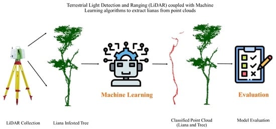
:Lianas are self-supporting systems that are increasing their dominance in tropical forests due to climate change. As lianas increase tree mortality and reduce tree growth, one key challenge in ecological remote sensing is the separation of a liana and its host tree using remote sensing techniques. This separation can provide essential insights into how tropical forests respond, from the point of view of ecosystem structure to climate and environmental change. Here, we propose a new machine learning method, derived from Random Forest (RF) and eXtreme Gradient Boosting (XGBoosting) algorithms, to separate lianas and trees using Terrestrial Laser Scanning (TLS) point clouds. We test our method on five tropical dry forest trees with different levels of liana infestation. First, we use a multiple radius search method to define the optimal radius of six geometric features. Second, we compare the performance of RF and XGBoosting algorithms on the classification of lianas and trees. Finally, we evaluate our model against independent data collected by other projects. Our results show that the XGBoosting algorithm achieves an overall accuracy of 0.88 (recall of 0.66), and the RF algorithm has an accuracy of 0.85 (recall of 0.56). Our results also show that the optimal radius method is as accurate as the multiple radius method, with F1 scores of 0.49 and 0.48, respectively. The RF algorithm shows the highest recall of 0.88 on the independent data. Our method provides a new flexible approach to extracting lianas from 3D point clouds, facilitating TLS to support new studies aimed to evaluate the impact of lianas on tree and forest structures using point clouds.
1. Introduction
Lianas are climber plants with woody stems, and they can climb to the forest canopy with the support of trees [1,2]. Although lianas occupy a small proportion (less than 10%) of the above-ground biomass in tropical forests [3], they represent a large percentage (up to 40%) of leaf productivity [1,4,5]. Apart from competing with trees for available resources [5], lianas also occupy gaps and illuminated areas on the upper part of the canopy more efficiently [2,6]. During the last two decades, liana abundance and biomass have experienced increases in tropical forests [7,8]. These increases tend to be associated with changes in forest structure [9]. An increase in liana abundance can suppress tree regeneration, promote tree mortality, and decrease tree growth, thereby causing a cascade effect on carbon storage, biodiversity, and primary productivity [10,11,12].
Unlike other structure parasites such as epiphytes and hemi-epiphytes, lianas grow their roots into the ground [13,14]. There are many growth strategies that lianas can link to their infested trees and grow to the forest canopy. Those strategies contain stem twining, clasping tendrils arising from the stem, leaf, and branch modification, downward-pointing adhesive hairs, adhesive adventitious roots, and thorns and spines that link lianas and trees [12]. The final climbing mechanism that lianas use from the above strategies is determined by the forest successional stages or disturbance level [12,15]. Since lianas have irregular growth forms, they contribute considerably to the architectural complexity of a given forest [5,16].
Many studies report the prevalence of lianas and their importance in tropical forests. However, few of them utilize quantitative methods to study their structure and their respective impact on an individual tree [17,18]. Recent advances in remote sensing techniques, in particular, Terrestrial Laser Scanning (TLS), provide a great opportunity to study the relationships between tree and liana structures in an unprecedented manner [9,19,20]. For instance, Moorthy et al. [17] investigated the potential utilization of TLS in monitoring changes in forest structure after liana removal, demonstrating that TLS could detect local structural changes after liana removal. Furthermore, Bao et al. [21] used TLS data and the Random Forest (RF) to classify lianas and trees with an overall accuracy of 94%. Although those studies present promising results, there are still uncertainties regarding the use of TLS to separate lianas from trees and extract them for their hosts. For example, as lianas grow towards a tree canopy, the stem diameter of most lianas is generally smaller than 10 cm, making it challenging to separate lianas and tree branches from a given point cloud. Additionally, lianas have a more irregular shape than trees, and they could grow around them in all directions randomizing the volumetric occupancy of the forest 3D space [9]. This attribute increases a TLS point cloud’s complexity, making lianas harder to separate and then study.
There are three approaches often used in previous studies to separate materials from the TLS point cloud: (1) those using radiometric features [22,23], (2) those using geometric features [24,25,26], and (3) combined use of both features [27]. Methods based on radiometric features depend on the type of TLS system used to generate a point cloud since the optical properties of a tree (e.g., wood or leaves) may respond differently to the LiDAR wavelength [26]. The x-, y-, and z-coordinates of each point are basic information of all LiDAR systems. Additionally, the geometric feature approach proves to be better than the radiometric method when comparing classification accuracies [28]. In the third method, a mixture of the two features mentioned above is used. Zhu et al. [27] applied the mixed approach to separate leaves from trees, achieving an average overall accuracy of 84%. This value was higher than using either radiometric or geometric features alone. However, this mixture method still has the disadvantage of relying on radiometric features [25].
Geometric feature methods are commonly derived from eigenvalues and eigenvectors calculated for each (x,y,z) point. A local neighborhood point set is required to obtain those features [29]. There are two approaches in terms of the definition of the local neighborhood of a point: k-nearest neighbors and radially bounded nearest neighbors. The former specifies a limited number of nearest neighbors for each point. In contrast, the latter approach defines a spherical space, and local point sets are within a given radius [27]. The radially bounded nearest neighbors approach is more advanced, since the k-nearest neighbors approach is often affected by the density of point clouds [26,28]. For instance, the canopy has a lower point density than the understory because of occlusion effects and the physical distance between the object and sensor [22]. As a result, using the same k-nearest neighbors approach, the geometry of leaves in the understory will be different from that in the canopy [25]. Moreover, Thomas et al. [30] indicated that the radially bounded nearest neighbors approach could allow the computed features (e.g., eigentropy, linearity, planarity, etc.) with a consistent geometric meaning, which is not possible for the k-nearest neighbors approach.
Concerning the radially bounded nearest neighbor approach, the size of the radius determines the local dimensional features of neighborhood points. For example, at a few centimeter scales, stem points are more likely to have surface features, while they tend to have linearly distributed ones at a large centimeter scale [28]. Using a single radius randomly selected to search for neighborhood points may not be reliable because the feature distribution of different objects varies in different situations [27]. This scale factor could be an important element to consider given how close lianas grow attached to a tree’s branch and trunk. A combination of the geometric features from all scales is also used in [31]. This strategy is shown to have a significant advantage compared to the single scale on leaf and wood classification. However, combing the features from all radii could produce many more of them than a single scale approach. Then, this multiple radius method would result in redundancy and low computational efficiency of the final model [32]. Selecting an optimal radius could be the right choice for classification purposes. Zhu et al. [27] applied an adaptive radius near-neighbor search method to select an optimal radius for each point, and then extracted the geometric features of those points to classify foliar and woody materials of a mixed forest. As their results suggested, the classification accuracy for adaptive radius near-neighbor search method was higher than that for the fixed radius near-neighbor search method.
There are many existing methods using machine learning to classify point clouds, while the purpose of most of those methods is to classify leaf and wood points [24,26,28,33]. Only a few studies use TLS data to discriminate lianas and their host trees in tropical forests. Moorthy et al. [16] presented a semi-automatic approach based on the Random Forest algorithm to separate liana from its host tree in Panama and French Guiana. Model recall of extracted liana stems increased after a manual intervention (54% to 90% and 65% to 70%, respectively) in [16]. However, many lianas in their study are away from the main trunk, and with a vertical distribution. When lianas are close to a tree’s main stem, and have more irregular shapes, their method cannot identify lianas successfully.
This work contributes to building a novel machine learning model based on Random Forests and Gradient Boosting algorithms, that can be used to separate lianas from trees. This method uses geometric features derived from point clouds. Our method extends and builds on the previous work of [16,24,31]. Furthermore, in this manuscript, we aim to answer the following questions: (1) Does the optimal radius method have significant advantages compared to the multiple radius method for liana/tree separation in [16]? (2) Do different machine learning methods affect the classification accuracy of lianas and trees? (3) Is our method more robust than other existing methods for 3D point cloud classification? We answer those questions using a set of liana and trees in a Tropical Dry Forest (TDF) with different infestation levels.
2. Materials and Methods
2.1. Study Area and Data
The original data come from the Santa Rosa National Park–Environmental Monitoring Supersite (SRNP–EMSS) (Figure S1), Guanacaste, Costa Rica [34]. The SRNP–EMSS has an average yearly temperature of 25 °C, and average yearly precipitation of 1720 mm. The SRNP–EMSS also has five months of the dry season (December to April), and a high biodiversity of plant and animal species, including 96 species of trees of different life histories, and 18 species of lianas among them [35].
We randomly selected five trees with different levels of liana infestation, and then used a Leica C10 TLS scanner (Leica Geosystem AG, Sankt Gallen, Switzerland) to scan those trees in May 2015 (end of the dry season). The Leica C10 TLS scanner uses green laser light with a wavelength of 532 nm, a maximum vertical field of view (FOV) of 270°, and a horizontal FOV of 360° [36]. The scanner collects 50,000 points per second at a range of up to 300 m [37].
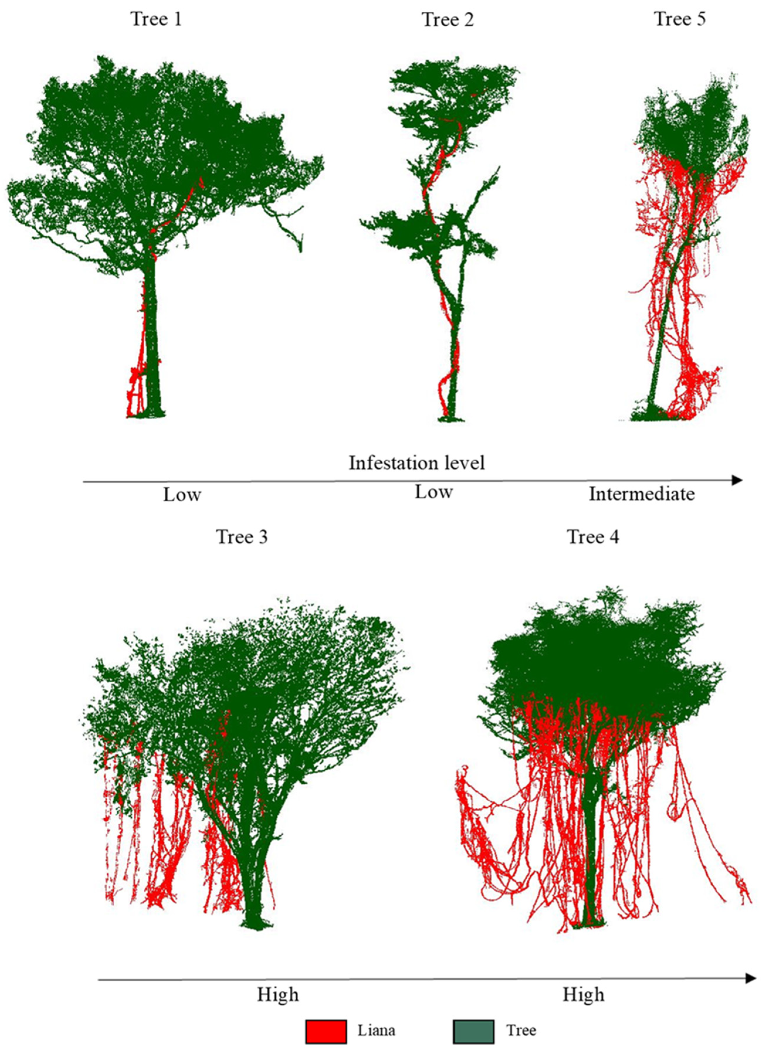
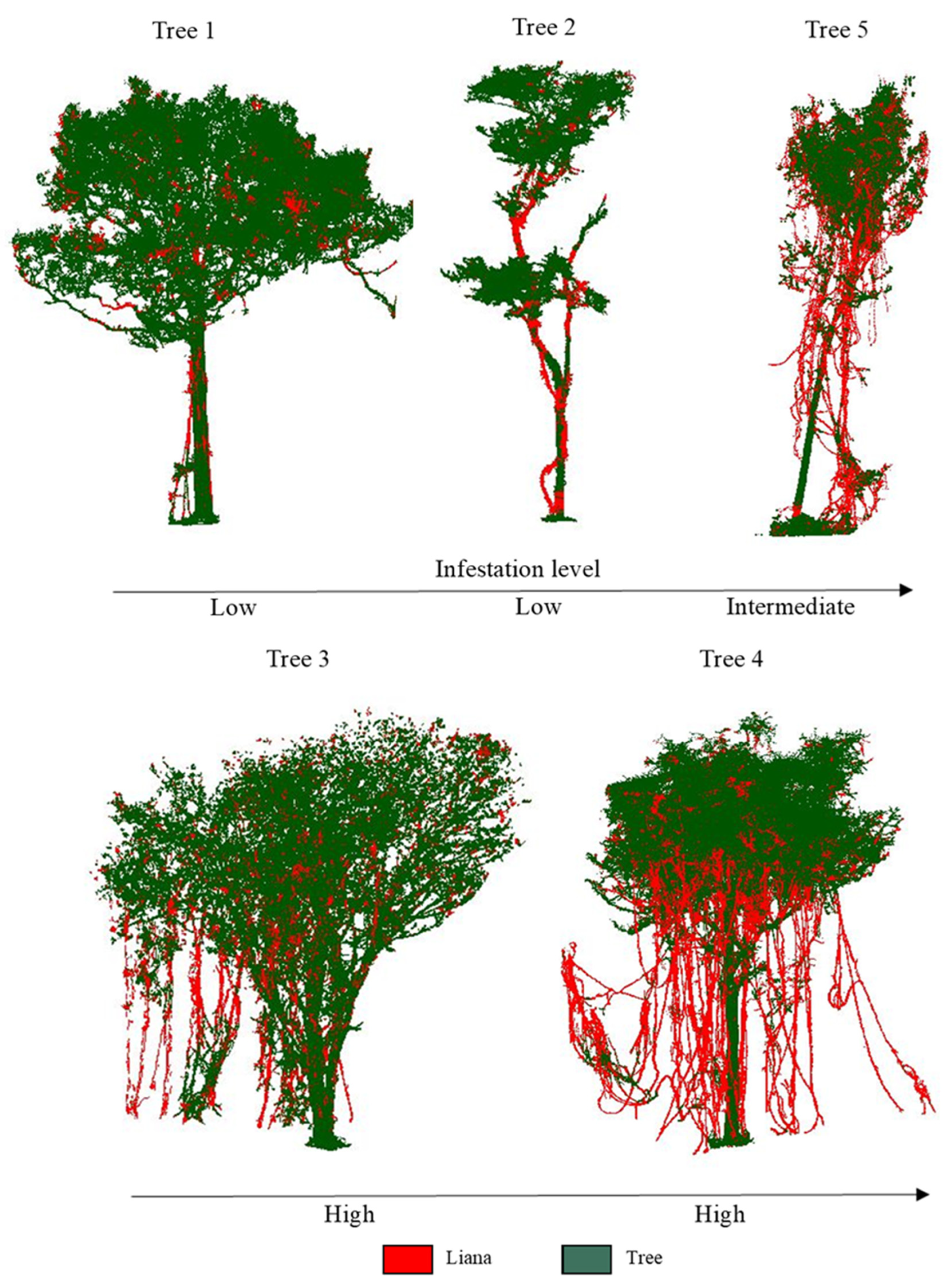
We selected four or five scan positions at a radius of 10 m to collect the TLS data. The location of scan positions was determined by where it was possible to show the highest visibility of the host tree and lianas. At least four reflective targets were used as control points to merge the point cloud from the four positions into a single high-resolution 3D datum, with fewer shadow effects [38]. This registration step was performed under the projected coordinate system (Cartesian) in Leica’s Cyclone software using the Iterative Closet Point (ICP) method (mean error of 0.02 m) [39]. The data collection process was carried out on sunny days with low wind conditions. A detailed description of all five trees is given in Table 1. Specifically, we used the Point Picking and Height Histogram functions in Cloud Compare software to obtain DBH and Height from the point cloud, respectively. Figure 1 presents the five trees with different infestation levels. The infestation levels were evaluated by professional dendrologists using standard forestry techniques.
We used an independent tree from Nouragues, French Guiana to test the performance of our method on unseen data. Specifically, Nouragues is a lowland moist tropical forest, which has a higher liana infestation [40]. Moorthy et al. [16] utilized a Riegl VZ-1000 scanner (RIEGL, Horn, Austria) to scan the target tree (August–October 2017). The Riegl VZ-1000 scanner uses a narrow infrared laser light with a wavelength of 1550 nm, a maximum vertical field of view (FOV) of 100°, and a horizontal FOV of 360° [41]. Specifically, five scan positions at a radius of 15 m are selected to obtain better visibility of the tree with liana infestation. Around 20 reflective targets were used to co-register the point cloud from those five positions to obtain single high-resolution 3D data [16].
2.2. Data Processing
2.2.1. Predictor Variables
Geometric features estimate local geometry by characterizing the distribution of neighboring points [16,27]. The proper estimation of geometric features requires using a covariance matrix, calculated from a local point set within a certain radius. Then, the three positive and ordered eigenvalues computed from the covariance matrix (λ1 ≥ λ2 ≥ λ3) can express how the local point set is distributed in the 3D space [28].
2.2.2. Data Labelling
The most crucial part of building the liana/tree classification model regarding supervised machine learning methods is labeling the training data. Here, we used Cloud Compare to manually mark the five trees into two classes, where class 1 and class 2 represented liana points, and tree points, respectively. To label the liana points, we visually follow lianas from the ground to the tree crown. This labelling process stops when we see lianas branch out to leaves. The data labelling process costs around 100 h. The proportion of liana points (an average of 8% of all the points) was much less than the proportion of tree points. This imbalance between liana on tree points has the potential to cause an unbalance weight in the model development [30]. Therefore, we randomly sampled 25% of all tree points to improve our classifier’s performance. As a result, tree points were two times as many as liana points in the final dataset for training and validation of the classifier.
2.2.3. Optimum Radius for Near-Neighbor Search
Some studies use a fixed radius to obtain the geometric features [28,44]. For example, the diameter at breast height (DBH) of a tree was used as reference to select a suitable searching radius to separate leaf and wood from a point cloud [44]. However, it is unlikely that the DBH is consistent across trees and plots, given that the DBH at the study site changes as a function of species and successional stage [45]. As such, we used a multiple radius search solution to define the optimal radius of the six features. This approach considers a heterogeneous DBH, while it could show a complete difference between the geometric features of liana and tree.
In this study, the geometric features in Table 2 were computed from 0.05 to 1 m, at a 0.01 m interval. A total of 96 values were created for each feature. We set up 0.05 m as minimum radius because we used a voxel grid filter with a size of 0.04 m to downsample our point cloud. There are two reasons why we select the size of 0.04 m to filter the voxel grid in this study. First, downsampling ensures that the distribution of points is uniform, which means high computational efficiency, although this may cause some information loss [46]. Second, the downsampling size in [16] is also equal to 0.04 m, allowing us to compare our study with the aforementioned paper. The maximum points were six at 0.05 m in this study. A radius beyond 1 m was also not considered, as this would need high computational memory. We used R studio [47] to randomly select five different numbers of liana and tree points. Then, we used Tree 2 to express how the geometric features of liana and tree changed from 0.05 to 1 m. As a result, five different curves for each class were obtained. We selected 100, 200, 300, 400, 500 points in the study. The final number of points was determined by observing whether there was stability among those five curves for each class. Here, 500 points were used to plot the changing trend of liana and tree for all features. The optimum radius was defined where the most considerable difference was shown between liana and tree curves. Specifically, we calculated the mean difference between liana and tree for each feature, and then find out the best radius that has the largest difference (see Supplementary Materials). Finally, we used all features at the optimum radius for the following classification.
2.2.4. Classification
Two ensemble learning classifiers, Random Forest (RF) and eXtreme Gradient Boosting (XGBoosting), are used to develop the liana extraction model. Ensemble learning classifiers combine many weak learners, such as decision trees, to form a strong one [48], and they show more advantages than other individual classifiers based on one strong learner [25]. The RF has the ability to limit overfitting. Additionally, considerable performance is obtained by RF when applied to leaf and wood classifications [27,43]. XGBoosting is a well-known classifier among a number of Gradient Boosting algorithms, while this classifier can show high performance on various tasks [49]. The implementation of the RF and XGBoosting algorithms, to separate lianas and trees from the different cloud points, was performed using the mlr R package [48].
In terms of the RF algorithm, there are four important hyperparameters: (1) the number of decision trees in the forest, (2) the number of random features to be sampled at each node, (3) the minimum number of cases allowed in a leaf, and (4) the maximum number of leaves. The grid search method is often used as a tuning tool since it can always find the best-performing hyperparameters [50]. However, since we have four hyperparameters here, using the grid search over this four-dimensional space requires much time and computational budget. Therefore, we used the random search method to find the best-performing hyperparameters. It should be noted that random search cannot always guarantee obtaining the best set of hyperparameters. In other words, it could find a good combination of hyperparameter values that performs well if we provide enough iterations. As such, 500 combinations of hyperparameters were run using the random search. Concerning the XGBoosting algorithm, there are eight hyperparameters to be tuned: (1) learning rate, (2) gamma, (3) max_depth, (4) min_child_weight, (5) subsample, (6) colsample_bytree, (7) nrounds, (8) eval_metric. Therefore, we run 1000 combinations of hyperparameters. We used 500 and 1000 combinations for RF and XGBoosting, respectively, based on the work of [48]. More details about hyperparameters and their optimization using RF and XGBoosting are given in supplementary materials.
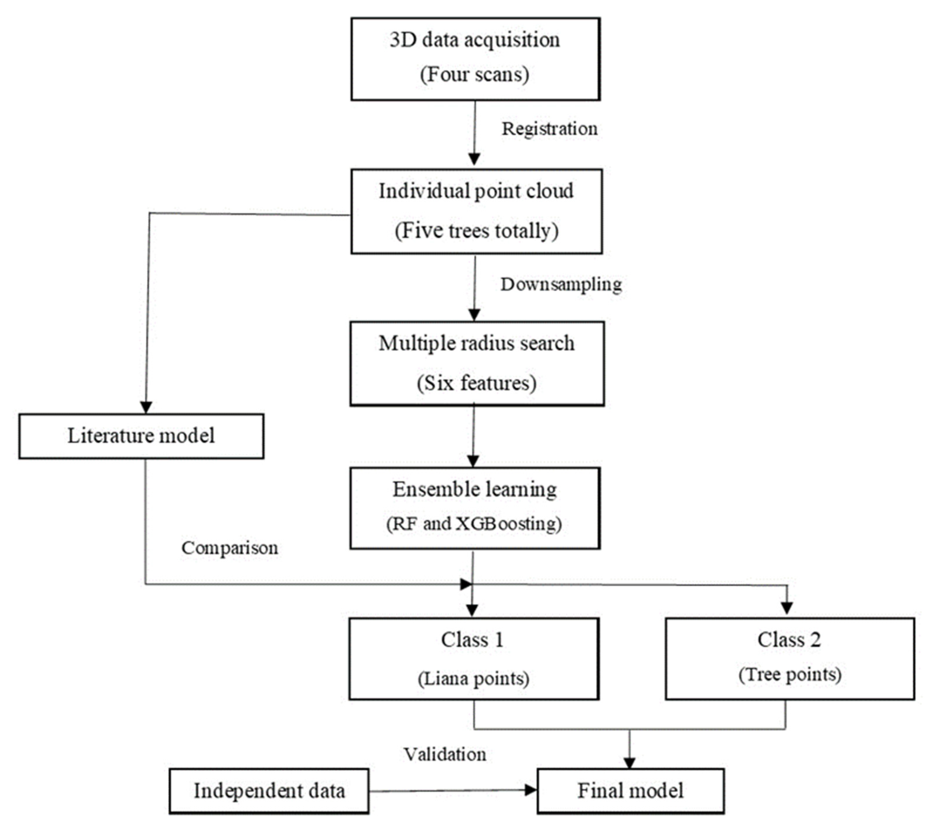
The performance of the model, including hyperparameter tuning, is evaluated using the k-fold spatial cross-validation method [48]. The model that has the optimal performance is therefore selected. The metrics described in Section 2.2.5 are used to assess the model performance. The complete pipeline of our methods is outlined in Figure 2.
2.2.5. Performance Assessment
We assess the performance of the presented liana/tree separation model using a k-fold spatial cross-validation method [16]. The k-fold spatial cross-validation strategy randomly splits the data into k-folds, while one fold at one time is used for validation, and the other unused k − 1 folds are used for training. In this study, we performed a five-fold cross-validation strategy to assess the performance of model, as shown in Figure S2.
The following metrics: Precision, Recall, F1 score, and Precision–Recall (PR) curve, were chosen to estimate our model’s performance [51]. The Precision is defined as the percentage of correctly predicted liana points (TP) divided by all classified liana points (TP and FP).
At the same time, Recall is the percentage of correctly predicted liana points (TP) divided by all real liana points (TP and FN).
F1 score is the balanced value between Precision and Recall (0 to 1), while 0 means the worst performance, and 1 is the best performance.
Accuracy is the proportion of all corrected classified lianas and tree points (TP and TN) against all points.
The Precision–Recall (PR) curve evaluates the trade-off between Precision and Recall for different liana point classification thresholds. The thresholds vary between 0 and 100% and are determined by the probability that the model estimates the positive class (liana point). The area under the PR curve shows the model’s performance, while the high value means both high Precision and Recall of the classifier.
2.3. Intercomparison with the Existing Method
We compared our method with [16], which used a multiple radius search method to obtain eigenvalues of each point at 0.1, 0.25, 0.5, 0.75, and 1.0 m. Then, the Random Forest method was selected to classify liana and tree based on those eigenvalues derived from point clouds. The details about running Moorthy et al. [16] are on GitHub (https://github.com/sruthimoorthy/automated-liana-extraction.git, accessed on 27 May 2019).
Four postprocessing steps were conducted in the above study to correct the misclassified liana points predicted by the RF model. First, a Statistical Outlier Removal (SOR) filter was applied in Cloud Compare to filter noisy points from the predicted liana class. Second, the components that did not belong to liana were manually removed by visual inspection using the polygonal selection tool. Third, a density-based clustering algorithm named DBSCAN was used to correct the liana points misclassified as wood in the model prediction. Given the number of points in space, DBSCAN could group the points together if the neighboring points are close enough. An additional description of this algorithm can be found in [52]. Isolated clusters classified as wood were achieved by applying the DBSCAN. Finally, DBSCAN was also applied to the corrected liana points in the second step, and liana points clusters were obtained. Those liana clusters were tested for connectivity with the wood clusters in the third step. If the wood cluster were very close to any liana clusters, they would be merged into single cluster using DBSCAN. The processing pipeline mentioned above was applied to the point clouds used in this study to understand the generalization of [16].
We evaluated the performance of our model on the independent data from Nouragues, French Guiana [16]. There are two reasons why we apply our method to these data. First, we want to indicate the broader utilization of our method, and second, we want to know whether our method shows more advantages than the former study.
3. Results
In this section, we first report the optimum radius for each geometric feature using the multiple radius search method. Then, we analyze the performance of the RF and XGBoosting models on liana and tree classification. Finally, we compare the generalization of our model with Moorthy et al. [16], the only existing method available in the literature applied to liana/tree classification.
3.1. Geometric Features Analysis
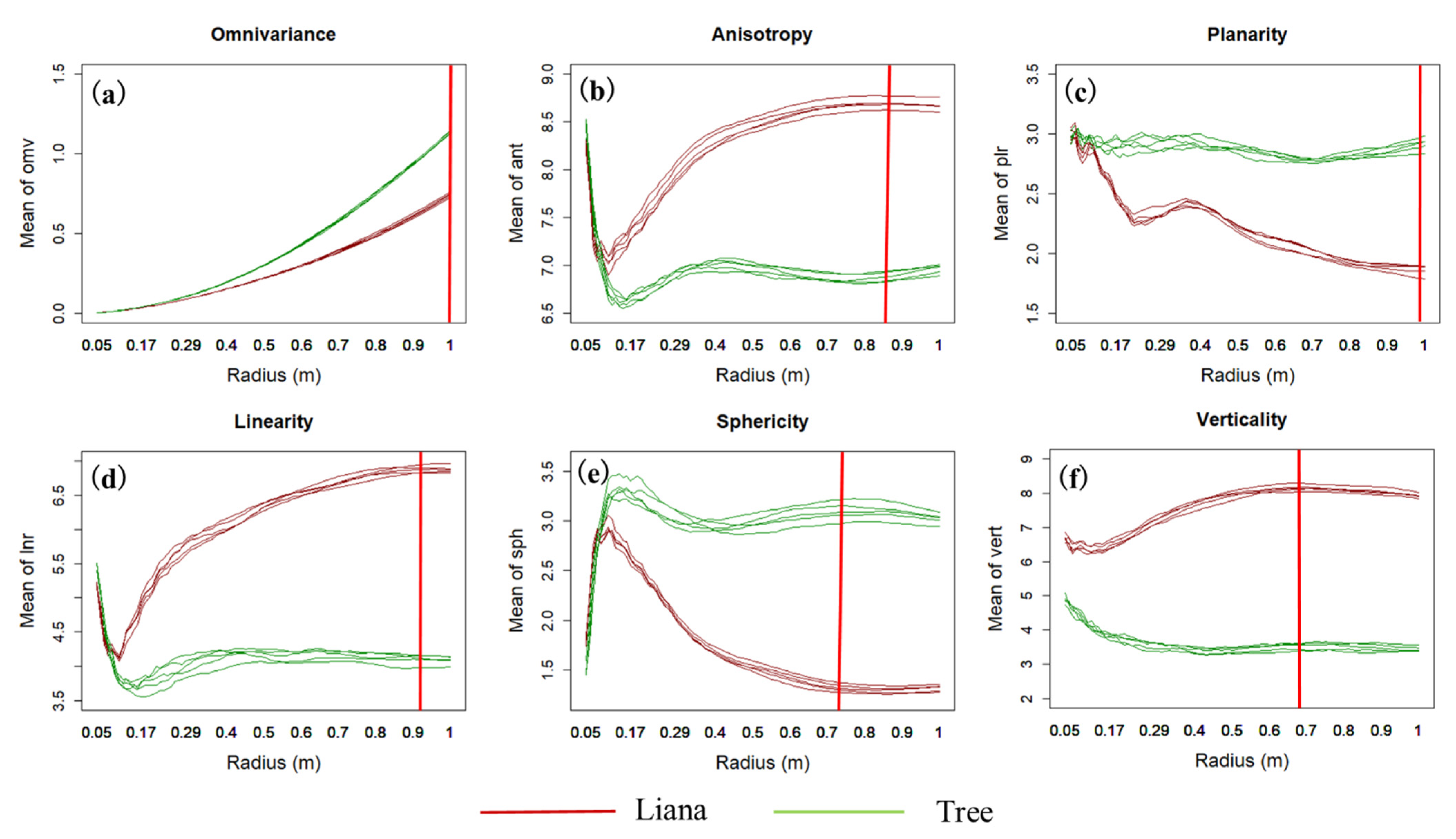
The optimum radius for determining the differences between lianas and trees for the remaining six features is detailed in Table 3. We can see that liana and tree points in Tree 2 tend to have a larger separability at the larger radius for all six features, while the verticality has the smallest radius of 0.68. The omnivariance is the only feature that shows the largest difference at 1 m across all trees collected due to the same increasing trend of liana and tree points. In addition, the optimal radii for Tree 2 are highlighted using red vertical lines in Figure 3.
Figure 3 presents the changing trends on the separation of lianas and trees for our selected six features for Tree 2 (Figure 1). The verticality is the only feature for which the mean value of liana is consistently higher than that of tree. Additionally, we can see that at the larger radius, the difference between liana and tree is similar (e.g., Anisotropy, Linearity, Sphericity and Verticality). A large number of points in the spherical space within a large radius could result in low computation efficiency when calculating geometric features. As such, we always select the smaller radius as the optimal one for classification (see also Figure S5). The changing trend of remaining trees can be found in Supplementary Materials.
3.2. Model Performance
To assess the effects of using an optimum radius for each feature, a five-fold cross-validation strategy that included hyperparameter tuning was applied. The details about the optimal hyperparameters of RF and XGBoosting used for this study are provided in the Supplementary Materials.
Table 4 presents all the performance metrics for the five-fold cross-validation strategy used for the classification of each infested tree. As shown in Table 4, both ensemble classifiers did not perform well on average, while the XGBoosting model performed better than RF. First, the overall accuracy of XGBoosting was 0.88 ± 0.07, which is higher than that of RF (0.85 ± 0.07) (p-value = 0.55, t = −0.62). Second, the average recall of Random Forest was 0.56 ± 0.17, 0.1 lower than the average recall of XGBoosting (0.66 ± 0.19) (p-value = 0.61, t = −0.53). The XGBoosting model based on the optimum radius of the features listed in Table 4 showed an average F1 score of 0.49 ± 0.24, with an individual score ranging from 0.19 to 0.75. The F1 score of the Trees 1, 2 and 3 in Table 4 was lower than 0.42, while Tree 2 had the highest recall, whether based on RF or XGBoosting model. The recall for Tree 4 was 0.8, with an F1 score of 0.75 for XGBoosting, the highest value of all trees. The final classification results of the XGBoosting model of five trees are presented in Figure 4. Compared with Figure 1, most lianas in Tree 4 were successfully predicted. Figure 4 also revealed that some parts of the stem were misclassified as liana, especially in Tree 2.
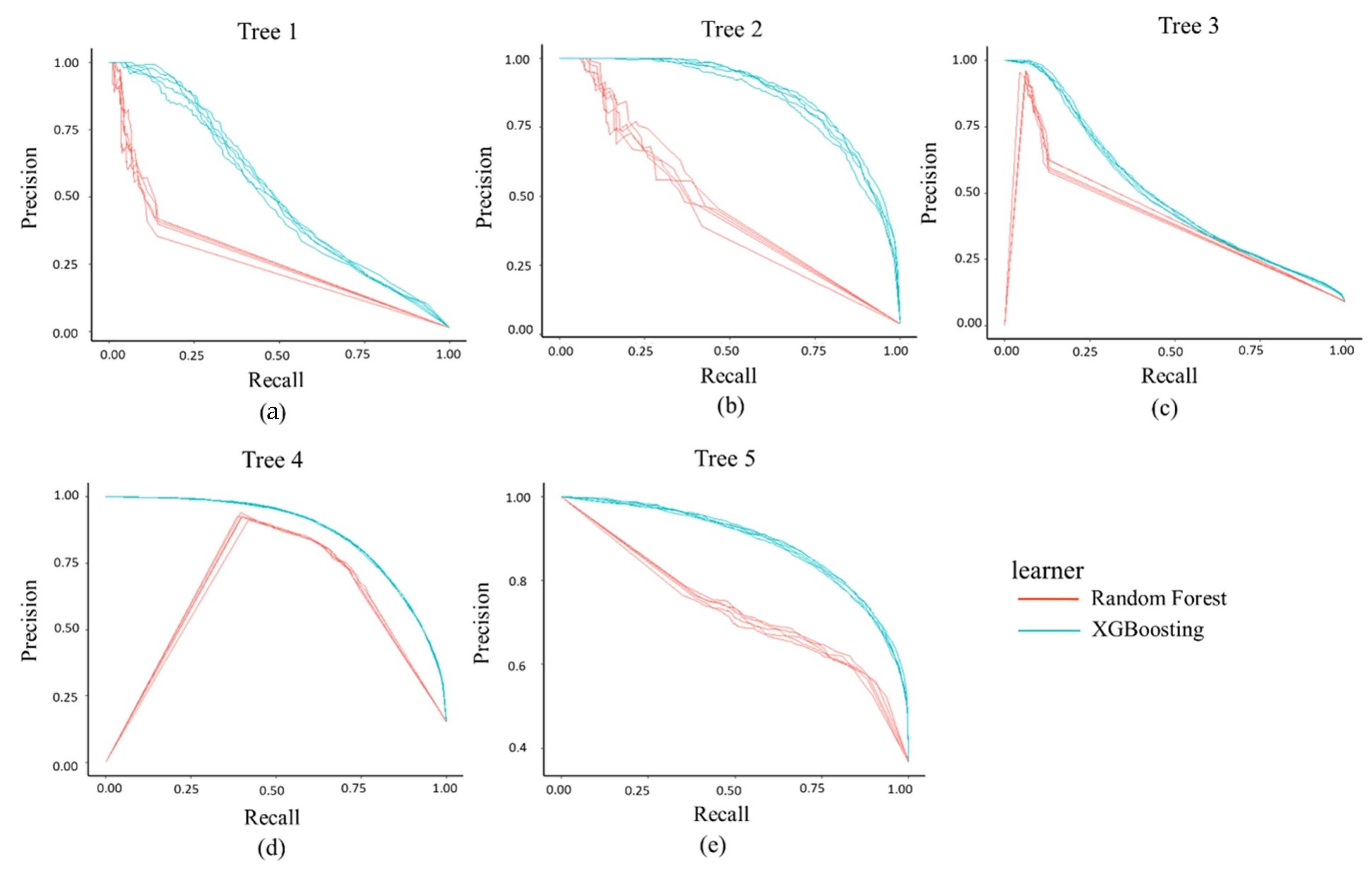
The Precision–Recall (PR) curve of the above two machine learning algorithms is shown in Figure 5, while the area under the PR curve for each tree is indicated in Table 4. Here, we compute the standard derivation of the areas under the PR curve of two methods for each tree to determine a stable pattern (see Table S1). Figure 5 indicates that the PR curve of RF and XGBoosting were more stable in Trees 3, 4 and 5 than that in Trees 1 and 2. Visual inspection from Figure 1 indicates lianas in Trees 3, 4 and 5 are vertically distributed, while lianas in the remaining two trees have close contact with the main stem. In addition, Table 4 reveals that the average area under the PR curve of XGBoosting for all trees is 0.72 ± 0.2, which is higher than that of the RF model (0.41 ± 0.29) (p-value = 0.08, t = −1.99).
3.3. Intercomparison
Our model’s performance was evaluated and compared with the only literature method for liana and tree classification [16]. Table 5 indicates the performance of their classifier on our datasets. Moorthy et al. [16] showed a poor performance for the five selected trees, the overall accuracy was 0.83 ± 0.12. After postprocessing suggested by [16], the method’s recall improved, with an average recall changing from 0.19 to 0.56, while the overall accuracy increased to 0.88 ± 0.07. Furthermore, the recall of Tree 4 and Tree 5 increased after the manual intervention, while Tree 4 had the highest value of 0.76. The method did not work for Tree 1 and Tree 2 since they had the lowest F1 score. Regarding postprocessing steps, DBSCAN generated a number of clusters ranging from 1, 600 to more than 17,000 for our trees (Table S2). Specifically, more than 17,000 clusters were obtained for Tree 4, while the number of points in Tree 4 was the largest of all trees (Table 1).
Compared with our method, the XGBoosting model performs similarly to [16], which combined the features from multiple neighborhood sizes (F1 score: 0.49 vs. 0.48).
The independent dataset (Nouragues, French Guiana) was used to evaluate our model on new unseen data. Table 6 compared the final recall for the dataset from the literature based on different methods. It was clear that our models, whether based on RF or XGBoosting algorithm, showed higher recall than the existing model without postprocessing (0.67). Though the recall of [16] improved to 0.87 after postprocessing, this showed a similar performance to the presented RF model’s recall (0.88).
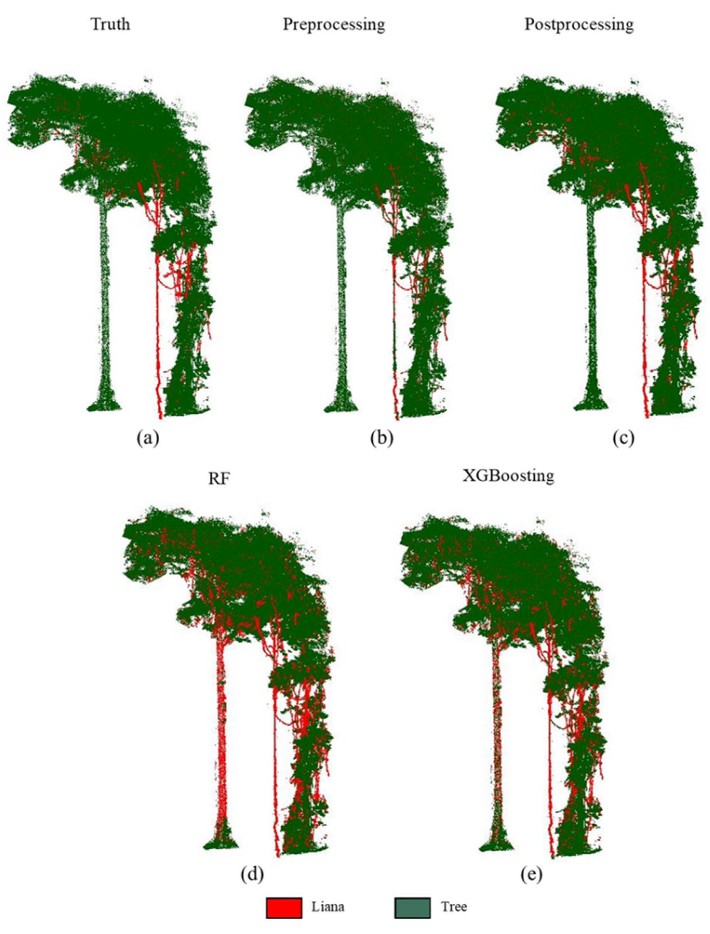
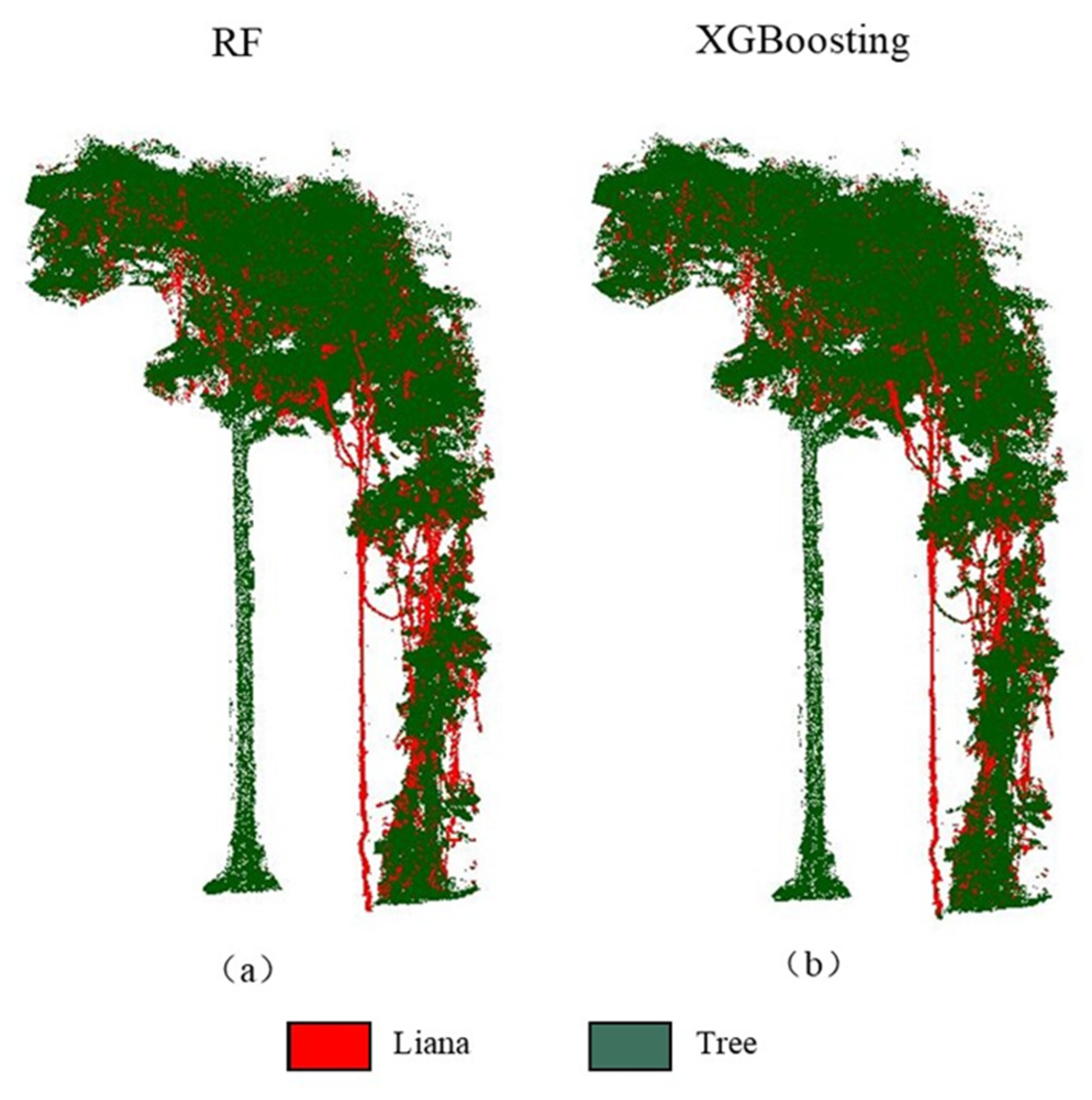
Figure 6 indicates the final predictions of different methods in Table 6 against independent data. It can be observed that RF (Figure 6d) and XGBoosting (Figure 6e) methods can also extract most lianas accurately, compared to the postprocessing method (Figure 6c). Although RF and XGBoosting methods misclassified some parts of the main trunk as lianas, this can be easily corrected by manual intervention, which can be seen from Figure 7.
4. Discussion
Here, we proposed a liana and tree classification method coupled with the geometric features of a tree/liana point cloud at the optimal radius. Furthermore, we compared our approach with the only literature method for liana and tree separation [16]. As shown in Table 4, the model based on XGBoosting showed a higher performance for all five trees. Table 6 further confirmed the advanced applicability of our method to independent data. For example, RF performed with a recall of 0.88 when tested on the independent data from the tropical forest in Nouragues, French Guiana (Figure 6) without postprocessing, and this value was the same as that for the state-of-the-art method after postprocessing (0.87).
4.1. Geometric Feature Analysis
The optimal radius near-neighbor search method was used to obtain geometric features. This method was superior to the multiple radius near-neighbor search for the discrimination of lianas and trees. According to Table 4, the average F1 score using the optimal radius based on the RF model was 0.41, which is higher than the multiple radius method (F1 score of 0.19) before the manual intervention. Although the average F1 score using the multiple radius method increased to 0.48 after using the postprocessing steps, this value was the same as our XGBoosting model without any postprocessing steps (F1 score of 0.49).
Our method suggests that the multiple radius method only works for Tree 4 from Table 5. The reason is that the liana structure of Tree 4 is vertically distributed, meaning that it has a similar shape to the independent data. Several reasons could explain why our method provides more advances when compared with [25,27]. First, although the multiple radius method could produce much more features than using only one scale [25], it may lead to redundancy. The former means that combining features from all radii could cause high-dimensional data. The optimal radius search method chooses the scale with the largest difference between liana and tree points at various radius, thus avoiding high-dimensional data. Second, our method described more detailed geometric features. For instance, Zhu et al. [27] computed the dimensional features for increasing radius values of 0.2, 0.3, and 0.4 m, and then determined the optimal radius based on Shannon entropy [29]. Searching only three radii may not be enough to define the optimum radius, which was a possible reason why their model obtained an overall accuracy of 70.4%. In this study, we determined the optimal radius from 0.04 to 1 m, at a 0.01 m interval. Then, we used a total of 96 radii to obtain the optimal radius, which had more quantities than the number of radius used in [27]. As a result, an overall accuracy of 85% and 88% was achieved for Random Forest and XGBoosting, respectively.
Using the multiple radius search method, Moorthy et al. [25] presented an improved supervised learning model to classify leaf and wood, achieving an overall accuracy of 94.2%. In addition, Ma et al. [28] used the single radius method, based on the improved salient features, to classify leaf and wood for conifer and broadleaf trees. Those geometric features gave the model an overall accuracy of 95.4%. Even though the performance of our method is lower than those implemented by the previous studies, this is related to the fact that these two studies look at simple structures while our liana/tree structure provides several levels of complexity (Figure 1). Lianas are climber plants with irregular growth patterns, which means that they could extend in all directions around their host trees [11,14]. This characteristic confuses the 3D deterministic nature of more simple forests [9], an element that is not considered on the trees analyzed by [25,28].
4.2. Liana-Tree Classification
Table 4 gives information about the performance of RF and XGBoosting on liana and tree classification. The XGBoosting method outperformed the RF method for the liana and tree classification on all five trees, and the overall accuracy and the average F1 score of XGBoosting model were higher than that of the RF model (0.88 vs. 0.85 and 0.49 vs. 0.41, respectively). Table 4 also reported the F1 score of Trees 1, 2 and 3 using the XGBoosting method was lower than 0.42. There are three reasons why those trees show worse performance. First, as liana stems move up to the canopy, their stems are of similar thickness as the tree components such as branches, and thus are misclassified; the former seems to be one of the current and future limitations on the use of TLS to extract lianas from their hosts, especially on the upper parts of the canopy. Second, lianas have close contact with the tree; therefore, it is challenging to distinguish liana and tree point even the optimum radius is applied. Third, lianas have a more complex structure than those in Tree 4. Lianas grow around the tree and ascend to the canopy for Tree 2 (Figure 1), thus showing much more curve structure than the liana structure in Tree 4. By contrast, the liana structure in Tree 4 is relatively simple, since most lianas on it are vertically distributed. This is the reason why Tree 4 shows the highest F1 score based on RF (0.71) or XGBoosting (0.75), same for [16].
4.3. Intercomparison with the Literature Method
We also compared our method with the only liana extraction method available in the literature [16]. The mentioned study used eigenvalues to separate liana and tree points, which showed clear disadvantages compared to eigenvalue-based ratios used in this study. The structure of lianas from their study is relatively simple, since their eigenvalues’ variance is dominant in one direction. However, this is not always the case. Lianas can grow in many different strategies, meaning that they tend to have more complex structures than stems or branches [9]. For example, the lianas in Tree 2 (Figure 1) grow around their host tree before moving up to the canopy. Therefore, the standard for liana and tree classification in their study may not work for our data. Their method only obtained an average recall of 0.19 before postprocessing steps, while this value increased to 0.56 after manual intervention (see Table 5). Instead, the ratios computed by eigenvalues could demonstrate how the lianas change in space. This is the one reason why our XGBoosting model shows higher performance, with an average recall of 0.66. When it comes to manual intervention, the density-based cluster algorithm (DBSCAN) spent much time recognizing the label of clusters [52]. For example, DBSCAN produced over 17,000 clusters for Tree 4 (Table S2), while the tree had the largest number of points of all trees (Table 1).
According to Table 6, our model’s final recall, whether based on Random Forest or XGBoosting, is higher than the state-of-the-art method without postprocessing. The manual intervention only improves the recall of their model to 0.87, showing similar performance to our model without postprocessing (0.88 of RF). Although our method misclassified some parts of the main stem as lianas (Figure 6d,e), this can be easily corrected using manual intervention. Figure 7 shows that our method, whether based on RF and XGBoosting algorithms, can extract most lianas from independent data after manual intervention. Therefore, our model’s performance shows that the presented method coupled with the curvature is more efficient for liana and tree classification than [16]. Our method’s major advantages are avoiding many postprocessing steps, while the performance of our method is also as accurate as that of previous studies. For instance, many isolated clusters (Table S2) need to be visually identified when using DBSCAN in [16] to obtain a reasonable performance, while our method can obtain the same performance without postprocessing. Moreover, the presented method avoids combining the geometric features at multiple radii, thus producing high-dimensional data. We calculate the geometric features of 96 radii to define the optimal radius, and this does not need much labor force, which can be performed using Cloud Compare and R programming. Additionally, we utilize geometric features to classify liana and tree cloud points, which means that the presented method only needs xyz coordinates, showing the broad applicability to the 3D point cloud collected from other sensors.
The highest F1 score of the proposed method is 0.49; the main reason is that the lianas’ structure is complex, while they are generally smaller than almost all the stems and show a diameter similar to branches. Due to their very irregular growth pattern, we suggest that it would be better if future researchers randomly select 500 points from liana and tree points first, and then define the optimal radius for further classification. This does not need much labor force and can also improve efficiency to extract lianas from point clouds, as indicated by our study. In addition, future work could pay attention to improving the performance of the algorithms for liana and tree classification. Recently, the development of more sophisticated machine learning technologies, especially deep learning, provides a solution to unstructured point clouds. Deep learning could extract features automatically to build a classifier, although it requires a large amount of data and high computational power [53]. Therefore, deep learning could be one of the solutions to improving the algorithm’s performance for liana and tree classification.
5. Conclusions
We present an open-source semi-automated liana extraction procedure (https://github.com/than2/liana-extraction, accessed on 1 September 2021) from point clouds derived from TLS data. Our approach avoids high-dimensional data and much manual intervention, making the entire procedure user-friendly and more efficient. Future research can pay more attention to improving the performance of liana extraction. For example, since we have the changing trend of liana and tree points from 0.05 to 1 m, time series classification can be used to separate them directly, which means that more radius information can be used during the classification. Although time series classification may produce many more features, this problem can be handled well by Convolutional Neural Networks and Recurrent Neural Networks. Our method can help in understanding the contribution of lianas to forest structure by an accurate segmentation/classification from point clouds.
Furthermore, it may provide a flexible approach to continuously monitoring liana dominance, enabling a better understanding of their role in the forest dynamics.
Supplementary Materials
The following supporting information can be downloaded at: https://0-www-mdpi-com.brum.beds.ac.uk/article/10.3390/rs14164039/s1. The supplementary materials mainly provide the following information: (1) the location of the study area; (2) the changing trends of the six geometric features for Trees 1, 3, 4, 5 and the independent data; (3) the numbers of cluster generated by DBSCAN on Trees 1, 2, 3, 4 and 5; (4) Hyperparameter used for RF and XGBoosting algorithms.
Author Contributions
T.H. and G.A.S.-A. presented and designed the experiments; T.H. carried out the experiments, analyzed the data and wrote the original paper. G.A.S.-A. contributed to reviewing and editing. All authors have read and agreed to the published version of the manuscript.
Funding
This research was funded by the National Science and Engineering Research Council of Canada (NSERC) Discovery Grant.
Data Availability Statement
Data used in this study and scripts used for analyses will be archived in the Tropi-Dry Dataverse repository, and the data DOI will be included at the end of the article upon publication. Currently, all files are attached as appendices for review.
Acknowledgments
The LiDAR instrument and data processing workstation were provided by the Center for Earth Observation Sciences (CEOS) of U of A. We thank Felipe Alencastro for his assistance with data collection. The authors also thank Sruthi M. Krishna Moorthy for providing her data collected in Nouragues, French Guiana.
Conflicts of Interest
The authors declare no conflict of interest.
References
- Ingwell, L.L.; Joseph Wright, S.; Becklund, K.K.; Hubbell, S.P.; Schnitzer, S.A. The Impact of Lianas on 10 Years of Tree Growth and Mortality on Barro Colorado Island, Panama. J. Ecol. 2010, 98, 879–887. [Google Scholar] [CrossRef]
- Letcher, S.G.; Chazdon, R.L. Lianas and Self-Supporting Plants during Tropical Forest Succession. For. Ecol. Manag. 2009, 257, 2150–2156. [Google Scholar] [CrossRef]
- Durán, S.M.; Gianoli, E. Carbon Stocks in Tropical Forests Decrease with Liana Density. Biol. Lett. 2013, 9, 3–6. [Google Scholar] [CrossRef] [PubMed]
- Rodríguez-Ronderos, M.E.; Bohrer, G.; Sanchez-Azofeifa, A.; Powers, J.S.; Schnitzer, S.A. Contribution of Lianas to Plant Area Index and Canopy Structure in a Panamanian Forest. Ecology 2016, 97, 3271–3277. [Google Scholar] [CrossRef]
- Schnitzer, S.A. A Mechanistic Explanation for Global Patterns of Liana Abundance and Distribution. Am. Nat. 2005, 166, 262–276. [Google Scholar] [CrossRef]
- Sánchez-Azofeifa, G.A.; Castro-Esau, K. Canopy Observations on the Hyperspectral Properties of a Community of Tropical Dry Forest Lianas and Their Host Trees. Int. J. Remote Sens. 2006, 27, 2101–2109. [Google Scholar] [CrossRef]
- Schnitzer, S.A.; Estrada-Villegas, S.; Wright, S.J. The Response of Lianas to 20 Yr of Nutrient Addition in a Panamanian Forest. Ecology 2020, 101, e03190. [Google Scholar] [CrossRef]
- Wright, S.J. Tropical Forests in a Changing Environment. Trends Ecol. Evol. 2005, 20, 553–560. [Google Scholar] [CrossRef]
- Sánchez-Azofeifa, G.A.; Guzmán-Quesada, J.A.; Vega-Araya, M.; Campos-Vargas, C.; Durán, S.M.; D’Souza, N.; Gianoli, T.; Portillo-Quintero, C.; Sharp, I. Can Terrestrial Laser Scanners (TLSs) and Hemispherical Photographs Predict Tropical Dry Forest Succession with Liana Abundance? Biogeosciences 2017, 14, 977–988. [Google Scholar] [CrossRef]
- Gonzalez de Tanago, J.; Lau, A.; Bartholomeus, H.; Herold, M.; Avitabile, V.; Raumonen, P.; Martius, C.; Goodman, R.C.; Disney, M.; Manuri, S.; et al. Estimation of Above-Ground Biomass of Large Tropical Trees with Terrestrial LiDAR. Methods Ecol. Evol. 2018, 9, 223–234. [Google Scholar] [CrossRef]
- Schnitzer, S.A.; Bongers, F. Increasing Liana Abundance and Biomass in Tropical Forests: Emerging Patterns and Putative Mechanisms. Ecol. Lett. 2011, 14, 397–406. [Google Scholar] [CrossRef] [PubMed]
- Schnitzer, S.A.; Bongers, F. The Ecology of Lianas and Their Role in Forests. Trends Ecol. Evol. 2002, 17, 223–230. [Google Scholar] [CrossRef]
- Gentry, A.H. The Distribution and Evolution of Climbing Plants. In The Biology of Vines; Cambridge University Press: Cambridge, UK, 1992; pp. 3–50. [Google Scholar]
- Schnitzer, S.A. Testing Ecological Theory with Lianas. New Phytol. 2018, 220, 366–380. [Google Scholar] [CrossRef] [PubMed]
- Dewalt, S.J.; Schnitzer, S.A.; Denslow, J.S. Density and Diversity of Lianas along a Chronosequence in a Central Panamanian Lowland Forest. J. Trop. Ecol. 2000, 16, 1–19. [Google Scholar] [CrossRef]
- Moorthy, S.M.; Bao, Y.; Calders, K.; Schnitzer, S.A.; Verbeeck, H. Semi-Automatic Extraction of Liana Stems from Terrestrial LiDAR Point Clouds of Tropical Rainforests. ISPRS J. Photogramm. Remote Sens. 2019, 154, 114–126. [Google Scholar] [CrossRef] [PubMed]
- Moorthy, S.M.; Calders, K.; di Porcia e Brugnera, M.; Schnitzer, S.; Verbeeck, H. Terrestrial Laser Scanning to Detect Liana Impact on Forest Structure. Remote Sens. 2018, 10, 810. [Google Scholar] [CrossRef]
- Londré, R.A.; Schnitzer, S.A. The Distribution of Lianas and Their Change in Abundance in Temperate Forests over the Past 45 Years. Ecology 2006, 87, 2973–2978. [Google Scholar] [CrossRef]
- Calders, K.; Newnham, G.; Burt, A.; Murphy, S.; Raumonen, P.; Herold, M.; Culvenor, D.; Avitabile, V.; Disney, M.; Armston, J.; et al. Nondestructive Estimates of Above-Ground Biomass Using Terrestrial Laser Scanning. Methods Ecol. Evol. 2015, 6, 198–208. [Google Scholar] [CrossRef]
- Calders, K.; Adams, J.; Armston, J.; Bartholomeus, H.; Bauwens, S.; Bentley, L.P.; Chave, J.; Danson, F.M.; Demol, M.; Disney, M.; et al. Terrestrial Laser Scanning in Forest Ecology: Expanding the Horizon. Remote Sens. Environ. 2020, 251, 112102. [Google Scholar] [CrossRef]
- Bao, Y.; Moorthy, S.; Verbeeck, H. Towards Extraction of Lianas from Terrestrial Lidar Scans of Tropical Forests. Int. Geosci. Remote Sens. Symp. 2018, 2018, 7544–7547. [Google Scholar] [CrossRef]
- Béland, M.; Baldocchi, D.D.; Widlowski, J.L.; Fournier, R.A.; Verstraete, M.M. On Seeing the Wood from the Leaves and the Role of Voxel Size in Determining Leaf Area Distribution of Forests with Terrestrial LiDAR. Agric. For. Meteorol. 2014, 184, 82–97. [Google Scholar] [CrossRef]
- Béland, M.; Widlowski, J.L.; Fournier, R.A.; Côté, J.F.; Verstraete, M.M. Estimating Leaf Area Distribution in Savanna Trees from Terrestrial LiDAR Measurements. Agric. For. Meteorol. 2011, 151, 1252–1266. [Google Scholar] [CrossRef]
- Tao, S.; Guo, Q.; Xu, S.; Su, Y.; Li, Y.; Wu, F. A Geometric Method for Wood-Leaf Separation Using Terrestrial and Simulated Lidar Data. Photogramm. Eng. Remote Sens. 2015, 81, 767–776. [Google Scholar] [CrossRef]
- Moorthy, S.M.; Calders, K.; Vicari, M.B.; Verbeeck, H. Improved Supervised Learning-Based Approach for Leaf and Wood Classification from LiDAR Point Clouds of Forests. IEEE Trans. Geosci. Remote Sens. 2020, 58, 3057–3070. [Google Scholar] [CrossRef]
- Vicari, M.B.; Disney, M.; Wilkes, P.; Burt, A.; Calders, K.; Woodgate, W. Leaf and Wood Classification Framework for Terrestrial LiDAR Point Clouds. Methods Ecol. Evol. 2019, 10, 680–694. [Google Scholar] [CrossRef]
- Zhu, X.; Skidmore, A.K.; Darvishzadeh, R.; Niemann, K.O.; Liu, J.; Shi, Y.; Wang, T. Foliar and Woody Materials Discriminated Using Terrestrial LiDAR in a Mixed Natural Forest. Int. J. Appl. Earth Obs. Geoinf. 2018, 64, 43–50. [Google Scholar] [CrossRef]
- Ma, L.; Zheng, G.; Eitel, J.U.H.; Moskal, L.M.; He, W.; Huang, H. Improved Salient Feature-Based Approach for Automatically Separating Photosynthetic and Nonphotosynthetic Components Within Terrestrial Lidar Point Cloud Data of Forest Canopies. IEEE Trans. Geosci. Remote Sens. 2016, 54, 679–696. [Google Scholar] [CrossRef]
- Demantké, J.; Mallet, C.; David, N.; Vallet, B. Dimensionality based scale selection in 3D lidar point clouds. Int. Arch. Photogramm. Remote Sens. Spat. Inf. Sci. 2012, XXXVIII-5/W12, 97–102. [Google Scholar] [CrossRef]
- Thomas, H.; Goulette, F.; Deschaud, J.-E.; Marcotegui, B.; LeGall, Y. Semantic Classification of 3D Point Clouds with Multiscale Spherical Neighborhoods. In Proceedings of the 2018 International Conference on 3D Vision (3DV), Verona, Italy, 5–8 September 2018; IEEE: Piscataway, NJ, USA; pp. 390–398. [Google Scholar]
- Belton, D.; Moncrieff, S.; Chapman, J. Processing Tree Point Clouds Using Gaussian Mixture Models. ISPRS Ann. Photogramm. Remote Sens. Spat. Inf. Sci. 2013, 2, 43–48. [Google Scholar] [CrossRef]
- Koenig, K.; Höfle, B.; Hämmerle, M.; Jarmer, T.; Siegmann, B.; Lilienthal, H. Comparative Classification Analysis of Post-Harvest Growth Detection from Terrestrial LiDAR Point Clouds in Precision Agriculture. ISPRS J. Photogramm. Remote Sens. 2015, 104, 112–125. [Google Scholar] [CrossRef]
- Wang, D.; Brunner, J.; Ma, Z.; Lu, H.; Hollaus, M.; Pang, Y.; Pfeifer, N. Separating Tree Photosynthetic and Non-Photosynthetic Components from Point Cloud Data Using Dynamic Segment Merging. Forests 2018, 9, 252. [Google Scholar] [CrossRef]
- Sánchez-Azofeifa, G.A.; Kalácska, M.; do Espírito-Santo, M.M.; Fernandes, G.W.; Schnitzer, S. Tropical Dry Forest Succession and the Contribution of Lianas to Wood Area Index (WAI). For. Ecol. Manag. 2009, 258, 941–948. [Google Scholar] [CrossRef]
- Guzmán, Q.J.A.; Rivard, B.; Sánchez-Azofeifa, G.A. Discrimination of Liana and Tree Leaves from a Neotropical Dry Forest Using Visible-near Infrared and Longwave Infrared Reflectance Spectra. Remote Sens. Environ. 2018, 219, 135–144. [Google Scholar] [CrossRef]
- Feliciano, E.A.; Wdowinski, S.; Potts, M.D. Assessing Mangrove Above-Ground Biomass and Structure Using Terrestrial Laser Scanning: A Case Study in the Everglades National Park. Wetlands 2014, 34, 955–968. [Google Scholar] [CrossRef]
- Taheriazad, L.; Moghadas, H.; Sanchez-Azofeifa, A. Calculation of Leaf Area Index in a Canadian Boreal Forest Using Adaptive Voxelization and Terrestrial LiDAR. Int. J. Appl. Earth Obs. Geoinf. 2019, 83, 101923. [Google Scholar] [CrossRef]
- Côté, J.F.; Fournier, R.A.; Frazer, G.W.; Olaf Niemann, K. A Fine-Scale Architectural Model of Trees to Enhance LiDAR-Derived Measurements of Forest Canopy Structure. Agric. For. Meteorol. 2012, 166, 72–85. [Google Scholar] [CrossRef]
- Kankare, V.; Holopainen, M.; Vastaranta, M.; Puttonen, E.; Yu, X.; Hyyppä, J.; Vaaja, M.; Hyyppä, H.; Alho, P. Individual Tree Biomass Estimation Using Terrestrial Laser Scanning. ISPRS J. Photogramm. Remote Sens. 2013, 75, 64–75. [Google Scholar] [CrossRef]
- Schnitzer, S.A.; DeWalt, S.J.; Chave, J. Censusing and Measuring Lianas: A Quantitative Comparison of the Common Methods. Biotropica 2006, 38, 581–591. [Google Scholar] [CrossRef]
- Schneider, F.D.; Kükenbrink, D.; Schaepman, M.E.; Schimel, D.S.; Morsdorf, F. Quantifying 3D Structure and Occlusion in Dense Tropical and Temperate Forests Using Close-Range LiDAR. Agric. For. Meteorol. 2019, 268, 249–257. [Google Scholar] [CrossRef]
- Weinmann, M.; Urban, S.; Hinz, S.; Jutzi, B.; Mallet, C. Distinctive 2D and 3D Features for Automated Large-Scale Scene Analysis in Urban Areas. Comput. Graph. 2015, 49, 47–57. [Google Scholar] [CrossRef]
- Wang, D.; Hollaus, M.; Pfeifer, N. Feasibility of Machine Learning Methods for Separating Wood and Leaf Points from Terrestrial Laser Scanning Data. ISPRS Ann. Photogramm. Remote Sens. Spat. Inf. Sci. 2017, 4, 157–164. [Google Scholar] [CrossRef]
- Ma, L.; Zheng, G.; Eitel, J.U.H.; Magney, T.S.; Moskal, L.M. Determining Woody-to-Total Area Ratio Using Terrestrial Laser Scanning (TLS). Agric. For. Meteorol. 2016, 228, 217–228. [Google Scholar] [CrossRef]
- Calvo-Rodriguez, S.; Kiese, R.; Sánchez-Azofeifa, G.A. Seasonality and Budgets of Soil Greenhouse Gas Emissions From a Tropical Dry Forest Successional Gradient in Costa Rica. J. Geophys. Res. Biogeosci. 2020, 125, e2020JG005647. [Google Scholar] [CrossRef]
- Burt, A.; Disney, M.; Calders, K. Extracting Individual Trees from Lidar Point Clouds Using Treeseg. Methods Ecol. Evol. 2019, 10, 438–445. [Google Scholar] [CrossRef]
- R Core Team. R: A Language and Environment for Statistical Computing. R Project 2021. Available online: http://www.R-project.org/ (accessed on 18 July 2022).
- Rhys, H.I. Machine Learning with R, the Tidyverse, and Mlr; Manning: Shelter Island, NY, USA, 2020; ISBN 9781617296574. [Google Scholar]
- Chen, T.; Guestrin, C. XGBoost. In Proceedings of the 22nd ACM SIGKDD International Conference on Knowledge Discovery and Data Mining, New York, NY, USA, 13–17 August 2016; ACM: New York, NY, USA, 13 August 2016; pp. 785–794. [Google Scholar]
- Lakicevic, M.; Povak, N.; Reynolds, K.M. Introduction to R for Terrestrial Ecology; Springer International Publishing: Cham, Switzerland, 2020; ISBN 978-3-030-27602-7. [Google Scholar]
- Tao, S.; Wu, F.; Guo, Q.; Wang, Y.; Li, W.; Xue, B.; Hu, X.; Li, P.; Tian, D.; Li, C.; et al. Segmenting Tree Crowns from Terrestrial and Mobile LiDAR Data by Exploring Ecological Theories. ISPRS J. Photogramm. Remote Sens. 2015, 110, 66–76. [Google Scholar] [CrossRef]
- Ferrara, R.; Virdis, S.G.P.; Ventura, A.; Ghisu, T.; Duce, P.; Pellizzaro, G. An Automated Approach for Wood-Leaf Separation from Terrestrial LIDAR Point Clouds Using the Density Based Clustering Algorithm DBSCAN. Agric. For. Meteorol. 2018, 262, 434–444. [Google Scholar] [CrossRef]
- LeCun, Y.; Bengio, Y.; Hinton, G. Deep Learning. Nature 2015, 521, 436–444. [Google Scholar] [CrossRef]
Figure 1.
Trees with different liana infestations collected at the SRNP–EMSS, Guanacaste, Costa Rica; the red color indicates the lianas stem, while the green color is the tree.
Figure 1.
Trees with different liana infestations collected at the SRNP–EMSS, Guanacaste, Costa Rica; the red color indicates the lianas stem, while the green color is the tree.

Figure 2.
The main steps used in the presented geometric method based on RF and XGBoosting algorithms for liana/tree separation.
Figure 2.
The main steps used in the presented geometric method based on RF and XGBoosting algorithms for liana/tree separation.

Figure 3.
The changing trends of Omnivariance, Anisotropy, Planarity, Linearity, Sphericity and Verticality for Tree 2 across the various radii (y-axis indicates the mean value of each feature, and the x-axis shows the value of radius from 0.05 to 1 m; red line: liana; green line: Tree); red vertical line indicates the optimal radius used in this study (see Table 3).

Figure 4.
XGBoosting model prediction for five trees. The prediction of Tree 4 tends to have a good consistency with the true data in Figure 1, while some parts of the stem in Tree 2 are misclassified as liana.
Figure 4.
XGBoosting model prediction for five trees. The prediction of Tree 4 tends to have a good consistency with the true data in Figure 1, while some parts of the stem in Tree 2 are misclassified as liana.

Figure 5.
Precision–Recall areas of each evaluated tree based on Random Forest and XGBoosting algorithms. The red and blue colors indicate Random Forest and the XGBoosting model, respectively. The area under the Precision–Recall curve means the performance of the classifier.
Figure 5.
Precision–Recall areas of each evaluated tree based on Random Forest and XGBoosting algorithms. The red and blue colors indicate Random Forest and the XGBoosting model, respectively. The area under the Precision–Recall curve means the performance of the classifier.

Figure 6.
The predictions of different methods in Table 6, (a) Truth: manual labeled; (b) Preprocessing: Moorthy et al. [16] without manual intervention; (c) Postprocessing: Moorthy et al. [16] with manual intervention; (d) Proposed method based on RF algorithm; (e) Proposed method based on XGBoosting algorithm.

Figure 7.
The proposed method based on RF and XGBoosting algorithms after manual intervention. (a) RF predictions after manual intervention, (b) XGBoosting predictions after manual intervention.
Figure 7.
The proposed method based on RF and XGBoosting algorithms after manual intervention. (a) RF predictions after manual intervention, (b) XGBoosting predictions after manual intervention.


Table 1.
Description of the trees with liana infestation collected in Santa Rosa National-Park Environmental Monitoring Supersite, Costa Rica.
Table 1.
Description of the trees with liana infestation collected in Santa Rosa National-Park Environmental Monitoring Supersite, Costa Rica.
| Tree ID | Tree Stem | DBH (cm) | Height (m) | Liana Infestation Levels | Liana Points Proportion | Number of Total Points |
|---|---|---|---|---|---|---|
| Tree 1 | 1 | 54.10 | 16.49 | Low | 1% | 405,262 |
| Tree 2 | 1 | 30.70 | 14.51 | Low | 4% | 121,954 |
| Tree 3 | 1 | 28.90/31.20/38.40 * | 16.57 | High | 9% | 382,599 |
| Tree 4 | 1 | 55 | 17.10 | High | 15% | 622,967 |
| Tree 5 | 1 | 20.50 | 13.96 | Intermediate | 37% | 87,346 |
* Three DBH values, for Tree 3 due to the three separated stems at breast height (1.3 m).
Table 2.
Six geometric features extracted from the point cloud. z represents the height of the point cloud, nv is the normal vector, and the eigenvalues.
Table 2.
Six geometric features extracted from the point cloud. z represents the height of the point cloud, nv is the normal vector, and the eigenvalues.
| No. | Feature | Description |
|---|---|---|
| 1 | Omnivariance | 3√) |
| 2 | Anisotropy | |
| 3 | Planarity | |
| 4 | Linearity | |
| 5 | Sphericity | |
| 6 | Verticality |
Table 3.
Optimum radius for different features on the evaluated point clouds for Tree 2.
| Feature | Tree ID | |||||
|---|---|---|---|---|---|---|
| Tree 1 | Tree 2 | Tree 3 | Tree 4 | Tree 5 | Independent | |
| Omnivariance | 1.00 | 1.00 | 1.00 | 1.00 | 1.00 | 1.00 |
| Anisotropy | 1.00 | 0.86 | 0.98 | 0.50 | 0.45 | 0.37 |
| Planarity | 0.13 | 0.99 | 0.22 | 0.16 | 0.87 | 0.29 |
| Linearity | 0.18 | 0.91 | 1.00 | 0.40 | 0.21 | 0.33 |
| Sphericity | 1.00 | 0.73 | 1.00 | 0.51 | 0.21 | 0.37 |
| Verticality | 1.00 | 0.68 | 0.24 | 1.00 | 0.70 | 0.45 |
Table 4.
Comparison of all performance metrics using RF and XGBoosting model; Aa, average area under the Precision–Recall curve; Ave, average; Sd: standard derivation.
Table 4.
Comparison of all performance metrics using RF and XGBoosting model; Aa, average area under the Precision–Recall curve; Ave, average; Sd: standard derivation.
| Tree ID | Random Forest | XGBoosting | ||||||||
|---|---|---|---|---|---|---|---|---|---|---|
| Precision | Recall | F1 Score | Accuracy | Aa | Precision | Recall | F1 Score | Accuracy | Aa | |
| Tree 1 | 0.05 | 0.44 | 0.09 | 0.9 | 0.09 | 0.12 | 0.47 | 0.19 | 0.95 | 0.51 |
| Tree 2 | 0.2 | 0.72 | 0.31 | 0.88 | 0.35 | 0.29 | 0.77 | 0.42 | 0.9 | 0.86 |
| Tree 3 | 0.32 | 0.37 | 0.34 | 0.82 | 0.21 | 0.3 | 0.44 | 0.36 | 0.85 | 0.5 |
| Tree 4 | 0.68 | 0.74 | 0.71 | 0.91 | 0.73 | 0.7 | 0.8 | 0.75 | 0.91 | 0.86 |
| Tree 5 | 0.67 | 0.52 | 0.59 | 0.73 | 0.69 | 0.65 | 0.82 | 0.73 | 0.77 | 0.89 |
| Ave | 0.38 | 0.56 | 0.41 | 0.85 | 0.41 | 0.41 | 0.66 | 0.49 | 0.88 | 0.72 |
| Sd | 0.28 | 0.17 | 0.24 | 0.07 | 0.29 | 0.25 | 0.19 | 0.24 | 0.07 | 0.2 |
Table 5.
The performance of liana and tree classification on our data using [16].
Table 5.
The performance of liana and tree classification on our data using [16].
| Tree ID | Without Postprocessing | Postprocessing | ||||||
|---|---|---|---|---|---|---|---|---|
| Precision | Recall | F1 Score | Accuracy | Precision | Recall | F1 Score | Accuracy | |
| Tree 1 | 0.05 | 0.24 | 0.08 | 0.92 | 0.27 | 0.40 | 0.32 | 0.98 |
| Tree 2 | 0.10 | 0.06 | 0.08 | 0.94 | 0.12 | 0.46 | 0.19 | 0.85 |
| Tree 3 | 0.11 | 0.22 | 0.14 | 0.76 | 0.38 | 0.66 | 0.48 | 0.87 |
| Tree 4 | 0.64 | 0.37 | 0.47 | 0.87 | 0.76 | 0.76 | 0.76 | 0.92 |
| Tree 5 | 0.73 | 0.08 | 0.16 | 0.65 | 0.85 | 0.52 | 0.64 | 0.79 |
| Ave | 0.33 | 0.19 | 0.19 | 0.83 | 0.48 | 0.56 | 0.48 | 0.88 |
| Sd | 0.33 | 0.13 | 0.16 | 0.12 | 0.32 | 0.15 | 0.23 | 0.07 |
Table 6.
Final recall of different methods on the dataset from [16].
Table 6.
Final recall of different methods on the dataset from [16].
| Methods | Model Recall |
|---|---|
| Random Forest | 0.88 |
| Postprocessing | 0.87 |
| XGBoosting | 0.82 |
| Without postprocessing | 0.67 |
Publisher’s Note: MDPI stays neutral with regard to jurisdictional claims in published maps and institutional affiliations. |
© 2022 by the authors. Licensee MDPI, Basel, Switzerland. This article is an open access article distributed under the terms and conditions of the Creative Commons Attribution (CC BY) license (https://creativecommons.org/licenses/by/4.0/).
Share and Cite
MDPI and ACS Style
Han, T.; Sánchez-Azofeifa, G.A. Extraction of Liana Stems Using Geometric Features from Terrestrial Laser Scanning Point Clouds. Remote Sens. 2022, 14, 4039. https://0-doi-org.brum.beds.ac.uk/10.3390/rs14164039
AMA Style
Han T, Sánchez-Azofeifa GA. Extraction of Liana Stems Using Geometric Features from Terrestrial Laser Scanning Point Clouds. Remote Sensing. 2022; 14(16):4039. https://0-doi-org.brum.beds.ac.uk/10.3390/rs14164039
Chicago/Turabian StyleHan, Tao, and Gerardo Arturo Sánchez-Azofeifa. 2022. "Extraction of Liana Stems Using Geometric Features from Terrestrial Laser Scanning Point Clouds" Remote Sensing 14, no. 16: 4039. https://0-doi-org.brum.beds.ac.uk/10.3390/rs14164039
Note that from the first issue of 2016, this journal uses article numbers instead of page numbers. See further details here.