1. Introduction
The thermal pattern on the surface of the Earth is an essential variable for understanding climate and biochemical processes. Satellite Earth observation of land surface temperature (LST) has become an important source of information for studying contemporary climate change and associated overheating of the urban landscape. The phenomenon is known as urban heat island (UHI) and it occurs in cities where air temperature tends to be higher than in the surrounding semiurban or rural areas [
1,
2]. UHIs have fundamental impacts on regional climate [
3], water and air quality, vegetation growth, and species richness [
4,
5]. These factors, in turn, affect human health and well-being as more than half of the world population now lives in urban areas [
6]. Global warming may potentially lead to increased morbidity and mortality, energy consumption, and economic changes [
7,
8].
Despite the fact that UHI originates in the atmosphere, the air temperature is strongly controlled by the spatial pattern of LST. Although the studies of UHI based on measurement of air temperature provide an accurate picture of thermal gradients, these are often limited by the number of monitoring stations to relatively small areas [
9], thus such measurements of atmospheric UHI are usually insufficient in capturing fine-scale spatial variation of air temperature [
10,
11]. In contrast, the surface UHI (SUHI) [
10] describes the changes in temperature on the surface and strongly correlates with the material type and orientation of the surface to the incident solar energy. SUHI is primarily measured by satellite thermal remote sensing. Consistent and continuous observations of the Earth’s surface allows for studying the urban thermal environment at various spatial scales (urban regions, cities) and temporal scales (diurnal, seasonal).
For more than fifty years, satellite remote sensing has enabled mapping the LST over large spatial extents from continental to global scales. However, physical and technical constraints limited the thermal infrared sensing (TIR) to coarser spatial resolution than other multispectral bands of the same satellite sensor, i.e., visible and near-infrared (VNIR). This is a relatively coarse spatial resolution of TIR datasets; typically, the ground sampling distance of Earth observation TIR sensors ranges from 1000 m (e.g., Meteosat, AVHRR, MODIS) to 100 m (Sentinel-3, ASTER, Landsat 8 and 9 TIRS). While the latter resolve the difference of urban–rural LST on the regional level, they are not sufficient to capture local interactions of LST within cities in relation to the land cover heterogeneity [
12]. Higher spatial resolution of thermal sensing is needed to resolve urban features (streets, roads, buildings) to study microclimate and human comfort in urban areas [
13]. Many land monitoring applications require LST estimates over large spatial extents (30–300 km) and at fine spatial resolutions (30–10 m or less). Airborne or UAV surveys enable thermal mapping at much higher spatial resolution, below submeter level, and bring the possibility of planning surveys when conditions are optimal to meet [
14] the project requirements. However, airborne platforms are more suitable for relatively small areas in which LST does not change significantly during data acquisition [
15]. Thus, LST can be captured in fine spatial detail for a small area or in a coarse resolution for the entire region.
This constraint has been addressed by sharpening the TIR satellite imagery to a higher spatial resolution. These sharpening techniques are often termed as downscaling or disaggregation methods in previous publications. Numerous techniques have been developed in recent years to downscale the TIR imagery or LST datasets based on the statistical relationship between TIR and higher resolution VNIR spectral bands. Zhan et al. (2013) reviewed disaggregation methods of remotely sensed land surface temperature [
16]. Zhan et al. (2013) followed the methodology of Strahler et al. [
17] and divided DLST into two subbranches, including thermal sharpening (TSP) and temperature unmixing (TUM). The main difference is that TSP is used to obtain the LST of smaller resolution cells, while TUM aims at obtaining the LSTs of the existing elements within coarse resolution cells.
Several researchers have approached LST downscaling over vegetated or natural landscapes using the relationship between LST and vegetation indices, e.g., normalized difference vegetation index (NDVI), fractional vegetation cover (FVC), via linear or nonlinear regression techniques, and the results were reported to be reasonably accurate. Kustas et al. [
18] developed the TsHARP algorithm, disTrad (disaggregation of radiometric temperature) method based on a quadratic relationship between NDVI and LST that has been widely used in several studies. However, urban areas contain greater heterogeneity in land cover and the behavior of the LST pattern varies across the surface. Therefore, NDVI cannot explain all LST variations in urban regions, so various authors have further refined TsHARP using fractional vegetation cover rather than NDVI to sharpen LST [
19,
20,
21,
22]. In addition to vegetation, the spatial pattern of the LST is also affected by other factors (e.g., type of land cover, soil moisture, geographic location) motivating improvement in thermal sharpening accuracy by integrating other datasets, e.g., land use data [
23,
24,
25], albedo [
13], emissivity [
26,
27,
28], soil moisture [
29], and digital elevation model (DEM) data into the sharpening process [
30]. These studies suggest that the inclusion of predictors other than NDVI and vegetation cover has the potential to improve sharpening accuracy in complex landscapes.
To date, Landsat 8 (L8) or Landsat 9 (L9) provides thermal imagery with a 16-day revisit period in the highest resolution freely available for research of landscape and urban planning. The LST data are derived at 30 m resolution and freely available online. The Sentinel-2 (S2) mission provides multispectral imagery at 10 m resolution with a 5-day data collection frequency, however, without a thermal band. Integration between L8 or L9 and S2/MSI data provides a global average revisit of approximately 3 days, which allows for continuous monitoring of land cover and development of application data products at medium spatial resolution [
31]. The S2 data can also be used to downscale L8/L9 LST to 10 m spatial resolution [
32].
This paper aims to make use of the spectral bands of S2 to sharpen the LST derived from L8 thermal sensing. To our knowledge, this idea has not been explored much in published research. Other kinds of data had been involved but not the S2 (e.g., [
14,
18,
21]). Sánchez et al. (2020) [
32] used S2 data to downscale MODIS data of 1000 m resolution to 10 m resolution. MODIS has the advantage of daily coverage, but thermal data with such a large cell size are not particularly applicable in urban landscapes where the land cover is diverse on a fine-scale. Pu and Bonafoni (2021) [
33] argue that the difference between the downscaled LST and LST measured at the same (high) resolution is scale-dependent, i.e., subject to a scaling effect. Therefore, larger-cell LST data, such as the MODIS, are not suitable for urban studies with complex land cover structures over small areas. Our research contributes to this aspect by focusing on the determination of LST in an urban environment for which L8 LST of 30 m cell size is more relevant but can be improved by fusing with S2 data. Li et al. (2022) [
34] conducted a similar study by using Gaofeng-6 (Gf-6) imagery to downscale the L8 to 8 m. Despite the high spatial and spectral resolution of the Gf-6 data, this imagery is not easily publicly available as the ESA S2 data are worldwide. This fact makes S2 more suitable on a global scale to be applied to determine the urban land surface temperature at 10 m resolution.
Our downscaling approach adopts a standard, well-known and simple approach of multiple linear regression to increase the spatial resolution of land surface temperature (LST) derived from L8 imagery. The method was originally proposed by Kustas et al. (2003) [
18] exploiting the inverse relationship of NDVI and LST. Bonafoni et al. (2016) [
14] modified it for downscaling Landsat-5 TM thermal data with airborne thermal data for urban landscape using three predictor spectral indices: normalized difference vegetation index (NDVI), normalized difference built-up index (NDBI), and normalized difference water index (NDWI). For the simplicity and robustness of this approach, we implemented the downscaling method in Google Earth Engine to increase the ease of use and global availability to other users via the Internet. The tool enables decision makers in cities to generate temperature maps of the urban surface for a particular day, given the periodicity of L8/L9, S2, and the level of cloudiness.
2. Materials and Methods
2.1. Study Area
The presented approach of downscaling L8 LST is demonstrated in the study area of the Košice city, located in eastern Slovakia, Central Europe. According to the Urban Atlas 2012 of the Copernicus Land Monitoring Service [
35], the area comprises the historical city center with dense continuous urban fabric surrounded by industrial and commercial units, green urban areas, asphalt roads, the main railway station, and a part of the Hornád River that flows in the east (
Figure 1).
The total area of the city is approximately 244 km
2 with total population of almost 240,000 inhabitants [
36]. Agricultural land occupies 37.6%. Forest areas are highly represented, accounting for 30.8%, built-up areas occupy 19%, water areas 1.2%, and other areas 11.4% of the city area [
37]. The local climate is mild and continental, strongly seasonal, with warm and humid summers and severe winters, without long dry periods; the Köppen Climate Classification subtype is “Dfb” [
38]. The average annual temperature is around 11 °C, slowly increasing in the last decade, with less rainfall and, at the same time, measuring a greater amount of sunshine per year [
37]. The average monthly temperature varies between 19 and 20 °C in July and −3 and −4 °C in January [
39].
2.2. Data Sources
The workflow of the presented research makes use of multispectral satellite imagery continuously collected by two Earth observation missions, the Landsat mission by NASA [
40] and the Sentinel mission by ESA [
41]. Three separate cloud-free multispectral products acquired over the Košice area on 23 August 2018 were employed: Landsat 8 Operational Land Imager/Thermal Infrared Sensor (OLI/TIRS) (2 products) and MSI instrument onboard S2 satellite (one product).
Two spaceborne multispectral imagery datasets of the Landsat 8 OLI/TIRS sensors from 23 August 2018, 09:19:59 UTM were downloaded using the USGS EarthExplorer web service (
https://earthexplorer.usgs.gov) (accessed on 17 May 2019) [
42]. The Landsat 8 Collection 1 Level-2 Surface Reflectance product “LC08_L2SP_186026_20180823_20200831_02_T1” was used to derive selected spectral indices in 30 m spatial resolution and Landsat 8 Collection 1 Level-1 product “LC08_L1TP_186026_20180823_20180829_01_T1” was used to compute atmospherically corrected LST using the adapted methodology of inverting the radiative transfer equation. The Landsat 8 OLI/TIRS sensors are composed of eleven bands, nine of them in the visible and near-infrared (B1–B9), and two bands in the thermal infrared (TIRS) region, with a spectral range of 10.60–12.51 μm (B10–B11). Landsat 8 OLI/TIRS has a native spatial resolution of 30 m for the eight reflective bands (B1–B7, B9), 15 m for the panchromatic band (B8), and 100 m for the thermal bands (B10–B11).
The Sentinel-2 MSI Level-2A multispectral imagery product, also from 23 August 2018 “S2B_MSIL2A_20180823T094029_N0208_R036_T34UEV_20180823T122014” (tile 34UEV, acquisition time 9:40:29 UTM), was downloaded via the Copernicus Open Access Hub (
https://scihub.copernicus.eu/dhus/) (accessed on 17 May 2019) to derive spectral indices in 10 m spatial resolution [
43]. The Sentinel-2 Level-2A outputs are based on the Level-1B data and they are provided to users as atmospherically corrected to bottom-of-atmosphere (BOA) reflectance products.
The original data supplied as projected in the WGS84/UTM zone 34N cartographic system. Calculations were performed in ArcGIS 10.8.
To validate the results of LST downscaling, we used field measurements of kinetic surface temperature that originated within the study by Hofierka et al. [
44]. The authors used the Pt1000TG7/E temperature probe with a data logger by Comet for automatic recording of the kinetic surface temperature at 6 locations shown in
Figure 1. The device measurement accuracy is 0.15 °C and the measurement interval was set to 30 s from 4:00 to 17:00 UTC time on 25 June 2020. We selected measurements performed in six open-sky locations within the study area to represent various types of environmental settings (e.g., roofs, parking lots, walkways, parks).
2.3. Downscaling Approach
Landsat 8’s thermal infrared sensor (TIRS) allows for direct mapping of surface thermal radiance at moderate spatial resolution, i.e., at the native 100 m ground sampling distance, which is resampled to 30 m by the United States Geological Survey (USGS). Landsat Collection 1 products generated from L8 are distributed at a 30 m raster cell size. The thermal radiance can be converted to LST. However, given the coarse spatial resolution and long revisit period of this satellite, the resolution is not sufficient for routine LST calculation of urban areas with diverse land cover controlling the distribution of heat in cities. S2 provides multispectral image data in the visible and near-infrared wavelengths at 10 m cell size, used for computing various spectral indices. These bands capture the complexity of urban land cover in finer detail and provide a higher resolution alternative to those generated by L8 or 9. However, S2 does not record the TIR radiance of the land surface.
Figure 2 presents the procedure of defining the multiple linear model of the three spectral indices and LST derived from L8 data adopted from [
14]. This model is used to predict LST in a grid of 10 m cell size with spectral indices derived from S2 data as inputs.
The flowchart in
Figure 2 shows the main steps that can be described in detail as follows:
Three indices NDVI [
45], NDBI [
46], and NDWI [
47] were selected and derived from images of the L8 satellite (surface reflectance product) at a spatial resolution of 30 m, and also from images of the S2 satellite at a resolution of 10 m (except NDWI that was resampled from 20 to 10 m) [
48,
49,
50]. Green, red, near-infrared, and shortwave infrared 1 bands of 30 m spatial resolution from the Landsat 8 OLI sensor, and the S2 MSI bands (green, red, near-infrared bands of 10 m spatial resolution and shortwave infrared 1 bands of 20 m spatial resolution) were used in determining the three land cover indices: NDVI, NDBI, and NDWI, as shown in
Table 1. The thermal infrared band 11 with 100 m spatial resolution in L8 TIRS sensor was used for calculating the LST. For convenience in the LST downscaling calculation, L8 TIRS data (100 m resolution) were resampled into 30 m using the nearest neighbor method by simple raster data aggregation to coincide with L8 OLI data (30 m resolution). Subsequently, the three indices (NDVI, NDWI, and NDBI) with 30 m resolution were then estimated from the 30 m OLI images (
Figure 3). The final available output is the downscaled LST of 30 m resolution.
- b.
Calculating LST from Landsat 8 data
The LST was retrieved from L8 OLI/TIRS data by inverting the radiative transfer equation according to:
where L
(sens,λ) is the at-sensor spectral radiance of band 10 (W.m
−2.sr
−1.μm
−1), ε
λ is the land surface emissivity, B
λ (T
s) is Planck’s law/radiance of blackbody (W.m
−2.sr
−1.μm
−1) where T
s is the real LST (K), L
d is the downwelling atmospheric radiance, τ
λ is the total atmospheric transmission for the thermal infrared radiation recorded by band 10, and L
u is the upwelling atmospheric radiance. By assuming a Lambertian surface and by inversion of Planck’s law from Equation (1), and knowing the surface emissivity and atmospheric parameters B
λ (T
s), τ
λ, L
d, and L
u, it is possible to find LST [
51]. The atmospheric correction parameters were calculated using an online web-based tool of NASA (
http://atmcorr.gsfc.nasa.gov) (accessed on 5 June 2019) developed by Barsi et al. [
52] that takes the National Centers for Environmental Prediction modeled atmospheric profiles as inputs to the MODTRAN radiative transfer code for a given site and date [
53]. The following input parameters were used in our case: latitude = 48.717°, longitude = 21.259°, UTM time = 9:20, altitude = 230 m a.s.l., temperature = 27.7 °C, air pressure = 990.9 hPa (mbar), and relative humidity = 40%. The weather parameters were extracted from the database of the OGIMET service (
www.ogimet.com) (accessed on 5 June 2019) for 23 August 2018 at 9:00 UTM for Košice-airport. The resulting values for the atmospheric correction were interpolated to the set location as follows: τ = 0.78, L
u = 1.82 W·m
−2·sr
−1·µm
−1, and L
d = 3.00 W·m
−2·sr
−1·µm
−1. Land surface emissivity ε
λ, was estimated using the threshold method based on NDVI according to Zhang [
54].
The meteorological station Košice-airport is the only one in the city that provides official temperature data at hourly intervals. The air temperature at 9:20 was linearly interpolated from recordings at 9:00 and 10:00 UTC, 27.2 °C and 28.9 °C, respectively. The increase in air temperature between the S2 and L8 observations from 9:19:59 to 9:40:29 was not greater than 1.7 °C. Assuming the linear increase in air temperature, the change during the 20 min time lag was 0.56 °C. There are other weather stations, e.g., personal weather stations (PWS), on the territory of the city of Košice that provide more detailed temperature data, such as the meteorological station E3925 (48.72, 21.24), which is located in the city center and is also part of the Meteorological Assimilation Data Ingest System (MADIS). Temperature data from these PWS stations are available at
https://www.pwsweather.com/ (accessed on 28 July 2022) [
55]. A similar increase in air temperature (0.5 °C) as noted above is found based on data from this weather station between 9:24–9:39 UTC time (27.8–28.3 °C). This analysis suggests that the air temperature was not stable between the two moments of L8 and S2 imagery acquisitions, but we consider it to be insignificant, below the radiometric resolution of the L8 data and without significant strength to affect the results of the presented research.
- c.
Defining the model between LST and land cover indices
In the next stage of this work, it was important to define the statistical model between the spectral indices and the calculated LST derived from the L8 data. The freely available statistical software R (The R Project for Statistical Computing) [
56] was used for this purpose to establish a multiple linear regression model according to the study of Bonafoni et al. [
14], which dealt with downscaling Landsat land surface temperature retrieved from Landsat Thematic Mapper (TM) using a high-resolution aerial image over the urban area of Florence. The proposed downscaling approach is based on fitting a linear relation using three spectral indices (NDVI, NDBI, NDWI) derived from L8, acting together as predictors with LST as the predicted variable. All input raster layers were in 30 m resolution. Then, the equation for the LST calculation from L8 imagery was derived using the output coefficients (a
0 − a
3) to calculate the LST
30m in ArcMap software using Map Algebra—Raster Calculator:
LST
10m at the finer 10 m resolution is predicted by applying the model, Equation (2), where the input spectral indices from L8 are replaced with the spectral indices derived from S2 data (in 10 m spatial resolution). The following model was used:
where coefficients (a
0 − a
3) from Equation (2) are applied and NDVI
10m, NDBI
10m, and NDWI
10m are the spectral indices derived from S2 at 10 m resolution. The final LST
10m contains regression residuals ΔLST
10m added back to the downscaled map. In this way, the original, coarse-temperature field is recovered through reaggregation, and the spatial variability [
21] of the LST that depends on factors other than the predictors employed is taken into account [
18]. The grid of regression residuals is first calculated by subtracting the observed LST
obs from the modeled LST
30m at 30 resolution (from Equation (2)):
ΔLST
30m is then resampled to ΔLST
10m as a 10 m cell-size grid by convolution with a Gaussian kernel of 30 m size in ArcMap [
18].
The resulting LST10m layer was validated against surface temperature measurements. Additionally, a linear model of LSTobs and LST10m was inspected.
2.4. Implementation in the Google Earth Engine
Google Earth Engine (GEE) provides a powerful cloud computing platform and access to an extensive catalogue of petabytes of satellite imagery with capabilities for performing global scale analysis, allowing efficient geospatial analyses [
57]. GEE provides access and processing of data from public or their private catalogues to any user, thus accelerating scientific advancements. We used this platform to implement a slightly modified version of the downscaling algorithm described in
Section 2.3 to enable other users to generate LST products with higher spatial resolution for their area of interest based on L8 TIR and S2 imagery.
The production chain was fully coded in JavaScript using the Code Editor Platform in GEE. We used the atmospherically corrected Landsat 8 Collection 2 Level 2 Surface Reflectance dataset (Landsat 8 SR) “LANDSAT/LC08/C02/T1_L2” and Sentinel-2 MSI Level-2A dataset “COPERNICUS/S2_SR” (Sentinel-2A). The selection of the Collection 2 dataset was led by the fact that NASA cut of the supply chain for Collection 1 data and all the NASA data were reprocessed to Collection 2. Moreover, L9 data are available in Collection 2. The algorithm is fed with data with less than 5% cloud cover (the user can adjust this value as described below). Another difference in the GEE application comparing to the methodology applied in this work is the use of 3 × 3 convolutional Gaussian kernel for image filtering and the subsequent bicubic interpolation to 10 m resolution.
Figure 4 illustrates the processing chain for generating downscaled LSTs in 10 m spatial resolution.
In the first step, the developed GEE application requires 5 different input parameters: start and end date (to select the desired time frame), Landsat collection (to select whether to use the L8 or L9 image collection), and maximum cloud cover allowed for the image tiles and the region of interest (ROI). The default ROI setting is focused on Košice city. However, the user can change the location where the analysis is performed. The ROI is created using the Geometry Tools in the GEE, which allow users to move or delete and then delineate their own new geometric features, such as polygons, to be applied in the analyses. After defining the input parameters, the user can click on “Generate L8/9 and Sentinel-2 Image Collections” button to generate available image IDs. Based on this information, the list of L8/9 and S2 imagery IDs that meet the entry criteria are displayed under the button in the right panel. The users can select two image IDs from the resulting list—one ID for the L8/9collection and one for the S2 L2A—and enter their exact ID to the newly displayed text fields. Several Landsat 8/9 and S2 imagery may be available in a given time window; therefore, we recommend selecting data sets that were acquired on the same day. If images for L8/9 and S2 collections are not available on the same acquisition day, we recommend choosing the datasets by the closest acquisition time to account for similar spectral characteristics of the derived spectral indices from both satellites. After defining the image IDs on which to perform the analyses, these images are then used to calculate the NDVI, NDBI, and NDWI spectral indices for the L8/9 and S2 imagery.
The LST is then calculated at 30 m resolution using the L8/9 B10 surface temperature in degrees Celsius. The three spectral indices of L8/9 are then used to calculate the coefficients of the multiple linear regression model between these indices and the LST band. Next, these regression coefficients are used to calculate the downscaled LST using S2 NDVI, NDBI, and NDWI spectral indices in 10 m resolution. The regression residuals are then calculated, resampled to 10 m using the bicubic interpolation, and filtered using Gaussian convolution with a window size of 3 × 3 pixels (30 × 30 m). The resulting regression residuals are added back to the downscaled LST to achieve the final result. The user can visualize the following 6 images: Landsat 8/9 and S2 natural color images (RGB), original L8/9 LST in 30 m, downscaled LST to 10 m spatial resolution with and without assuming residuals, and Landsat 8/9 LST regression residuals.
3. Results
3.1. Linear Model of Spectral Indices and LST Derived from Landsat 8 Data
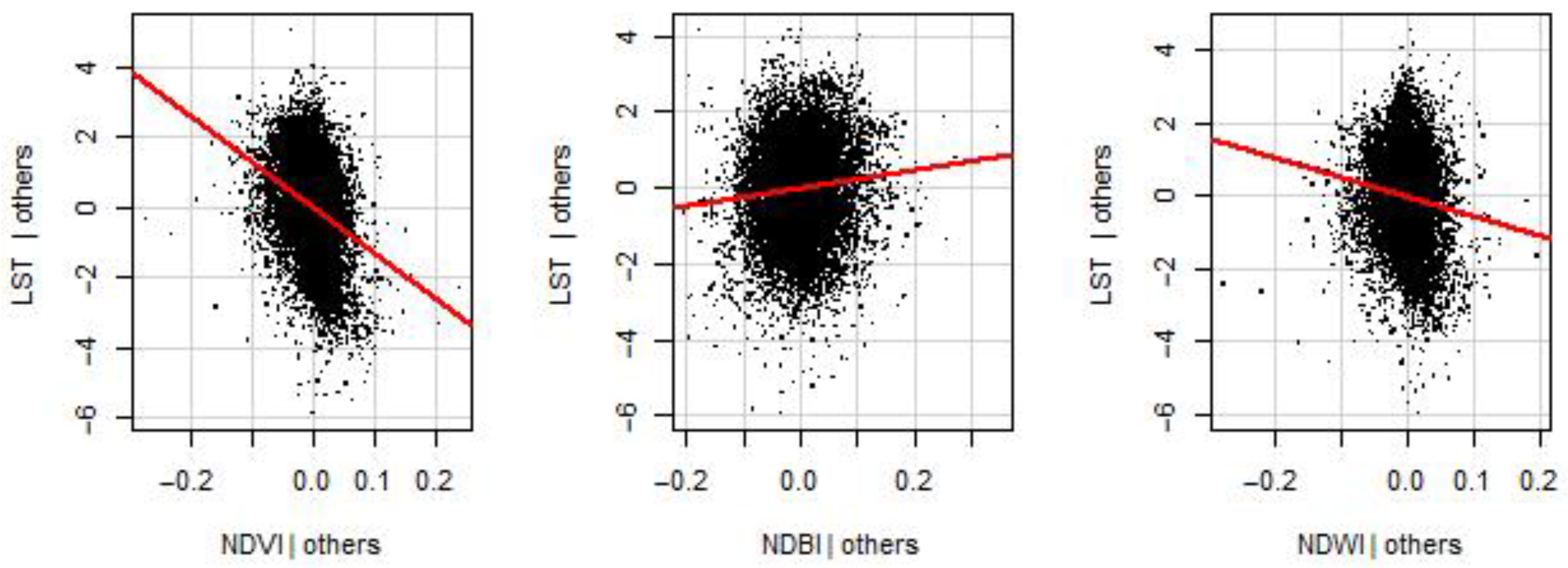
The model for LST prediction was defined based on three predictors and ordinary least squares linear regression similarly to [
18]. First, the bivariate relationship between L8 LST and each of the predictors was defined (NDVI, NDBI and NDWI, and LST) (
Figure 5).
Figure 5 shows a relation between pairs of variables separately. The scatter plots show that in the study area of Košice, there is a relatively strong relationship between the spectral indices and LST: negative for NDVI and positive for NDBI and NDWI. The coefficient of determination (R
2) is 0.63, 0.503, 0.564, respectively. The coefficient of determination shows that there is a significant degree of correlation. Owing to the high density of dots, they are displayed as probability density function (PDF) values. Minor deviations occur in the correlation between LST and NDVI, and between LST and NDWI. This can be caused by the use of atmospheric corrections and the derivation of surface emissivity values according to the methodology described in [
58], where these values were determined according to NDVI and were classified.
To define the relationship of all three spectral indices as an independent variable with LST (all variables in 30 m resolution), a linear regression model with three independent variables was created using the command (lm.output.lst < lm (lst ~ ndvi + ndbi + ndwi, temp.df). The equation for LST from L8 was derived from the output (see
Figure 5):
The coefficient of determination (R2) when using all three indices as independent variables is higher (R2 = 0.642, p-value < 0.0001) than the values of R2 for indices with LST30m in bivariate linear regression. The coefficients in Equation (5) were further used in the prediction of LST10m from S2 spectral indices.
Figure 6 shows a partial regression plot (i.e., added-variable plot). The graphs display the relationship between the independent variable on the x-axis while holding all other variables constant. It is an indication of the true relationship between variables in the multiple regression model of Equation (5).
3.2. Downscaled LST Using Sentinel-2 Data
LST
10m was derived by applying the Equation (3), which uses the coefficients in Equation (5). The procedure was performed in the ArcMap software environment using the Raster Calculator tool with the indices from S2 in 10 m spatial resolution:
Figure 7 shows the LST maps and residuals of the regression model Equation (2). The spatial pattern of the original LST
obs (
Figure 7A) is clearly improved (
Figure 7B) even before adding the residuals (
Figure 7C). The final LST
10m (
Figure 7D) contains the regression residuals. The difference of LST distribution can be clearly associated with particular land cover materials differing in temperature. A detailed view of the historical city center is shown in
Figure 8.
Figure 7 shows the highest values within the densely built-up historical center of the city with sharply distinguishable main roads and building blocks. Urban greenery such as parks and smaller or narrower green areas in the city, and industrial areas with vegetation are clearly visible as islands of lower LST. On the other hand, building blocks, roads, and railways are distinguishable as hotter surfaces. Such a sharpened map of LST has a higher interpretative value for public, urban planners, or researchers than the original LST
obs map.
Ideally, the LST
obs image (
Figure 7A and
Figure 9A) and the downscaled (sharpened) LST
10m image aggregated to the coarse native TIR resolution of 30 m (
Figure 9B) should be identical, i.e., there is no bias (residuals) between the original and the aggregated prediction. As the derived model of LST
30m is not perfect, the underlying model prediction is inaccurate and generates residuals (
Figure 7C). The available spectral bands and the generated three indices are missing all the information needed to perfectly reconstruct the LST at a finer resolution. Therefore, to enforce energy conservation within the sharpening process, residuals between predicted and observed LST fields at the coarse resolution are redistributed over the sharpened LST maps (
Figure 9B) [
59]. The residual analysis helps to evaluate the model performance.
Figure 9C shows the relation between LST
obs and the LST
10m aggregated to 30 m resolution. High coefficient of determination R
2 of 0.829 (
p < 0.0001) indicates a very good, though imperfect, reconstruction of the original LST observed by L8 with Pearson’s correlation of 0.91. Additionally, other published thermal sharpening techniques redistribute the LST residuals to ensure energy conservation in the sharpened imagery (i.e., ensure that the downscaled LST map aggregates to the original coarser resolution LST values). Very high or low residuals are observed at places where predictors act most strongly as most limiting the LST ranges. Alternatively, the residuals tend to increase in these areas because the underlying predictor values are more extreme. Positive residuals in
Figure 7C indicate that the recorded temperatures were higher than the predicted temperatures and are represented by the warmer hues of the image, while the cooler hues represent overestimation of the observed LST by the model.
3.3. Online Application for LST Downscaling Based on the Google Earth Engine
The production chain was completely coded in JavaScript using the GEE Code Editor Platform, and a GEE application was developed to easily reproduce the LST downscaling process for different dates and areas for researchers and general public. The GEE application is available at:
and the source code of the application is available from the GitHub repository:
While Equations (5) and (6) are valid for the area of the case study in Košice, the GEE implementation calculates multiple linear regression models specific for the region of interest defined by the user. The user can change the ROI for any place in the world. For a meaningful result, the ROI should not be too large; we recommend a maximum of 1000 km2. Additionally, instead of creating a new ROI, it is possible to move with the predefined ROI and area for random sampling included in the script simply by clicking and dragging by mouse. The user can visualize the following six images: downscaled LST to 10 m spatial resolution with and without assuming residuals—“LST 10 m (with residuals)”, “LST 10 m (no residuals)”, original L8/9 LST in 30 m (“Landsat 8/9 LST”), L8/9 LST regression residuals (“Landsat 8/9 LST regression residuals”), L8/9 and S2 natural color images (RGB) (“Sentinel-2 RGB”, “Landsat 8/9 RGB”). There is also the option to generate charts of spectral indices vs. Landsat LST.
Figure 10 shows an example of downscaled LST layer generated by the LST production chain in
Section 2.3; the data were acquired on 23 August 2018 for the area of Uzhgorod city, Ukraine. The highest LST values are visible in the built-up areas; on the contrary, the lowest LST values indicate forests, urban green areas, such as city parks, river, and fields.
3.4. Validation of Downscaled LST with In Situ Surface Temperature Data
Because Košice city currently lacks an adequate number of weather-station data, validation of downscaled LST results was performed using the Comet Pt1000TG7/E temperature probe measurements at six sites in the city to represent different types of land cover (
Table 2). We selected 25 June 2020 to manually measure LST in the city center, as this day was similar in atmospheric characteristics (temperature = 23.2 °C, relative humidity = 40%) to the day of the satellite imagery acquisition 23 August 2018 (temperature = 27.2 °C, relative humidity = 40%).
However, comparing the downscaled results to high-resolution observed information would highlight systematic biases and limitations of the results. Planning a manual measurement that is synchronous with the flight of both L8 and S2 satellites simultaneously over our territory, and at the same time so that there is no haze or clouds over the territory, is also personnel and implementation demanding. During the measurements made by manual data loggers in the summer of 2020, there was a small cloud cover over the city at the time of satellite scanning, which prevented the use of the results captured by these satellites to derive LST10m after downscaling; the images were partially covered by cloudiness, which could introduce an error into any LST10m derived from these images after downscaling, thus affecting the resulting values.
The validation was performed, but due to low clouds over the area and the effort not to bring the error into the derived final temperature LST10m after downscaling, we decided to compare our manually recorded information from temperature data loggers with LST10m into downscaling derived from cloudless images L8 and S2, which was a day with a similar temperature profile and atmospheric characteristics at the time of satellite scanning as the day on which the recording was performed manually by temperature recorders.
The summary in
Table 2 indicates a systematic underestimation (bias) of the surface kinetic temperature T
dat measured in situ and the observed LST
obs or downscaled LST
10m, by −2.05 °C and −1.55 °C, respectively. The closer match of the predicted LST
10m with the reference data is indicated also by a lower RMSE of 4.22 °C as opposed to 4.43 °C for LST
obs, as might be expected at measuring points that are more homogeneous in the immediate vicinity of the type of land cover, (i.e., where it does not occur in the vicinity another type of surface). As an example, we can mention LST measured in a pedestrian zone in the historic core of the city (station no. 4), which is paved with cobblestone, where the difference in surface temperature was recorded approximately in the middle of this pedestrian zone, i.e., with a predominance of one type of land cover. The difference between the value of the surface temperature measured by the manual temperature logger (T
dat) and the value of the corresponding LST
10m cell after downscaling for the same locality was in this case the lowest among the measured values of selected localities (less than −0.21 °C). A similar example can be the city park (station no. 5), where the difference between the values of the surface temperature T
dat and LST
10m was less than −0.7 °C (see
Table 2). On the contrary, the highest difference (−7.63 °C) between the values of T
dat and LST
10m can be observed at station no. 1, which represents the roof. The difference among the reference point data and predicted or observed LST can be attributed to the different spatial supports of these data. While the in-situ measurement recorded temperature at a point level the L8 and S2 acquire LST over an area where a strong aggregation effect exists. The LST of qualitatively different surfaces (e.g. concrete surface of the parking lot, roofs of surrounding buildings) is comprised in the resulting cell LST
10m in 10 m resolution generating an average LST value. On the other hand, the differences become smaller in case the same surface material is comprised within the entire cell, both for L8 and S2, and it is also measured in-situ on the same material. Therefore, Stations 4 and 5 (
Table 2) corresponded most closely with the L8 observed and the S2 predicted LST. The stations 1-3 had the largest LST difference for the cells comprising mixture of surface materials.
The results confirm that even the use of resolved surface properties, such as spectral indices from S2 in 10 m resolution, to derive LST cannot improve the original L8 satellite capability to resolve some thermal details. This is consistent with previous findings, e.g., [
14]. Nevertheless, the custom downscaling procedure provides an additional value by improving the spatial resolution with respect to the L8 USGS image and other regressive downscaling techniques.
The validation measurements are not optimal as they are not taken on the same day as the L8 satellite data used in this study. However, we opted for a Landsat scene and weather conditions that were very close to the day of the field measurements, 25 June 2020. In fact, the advantage of the field data used is that they were recorded at the same time moment for each of the six locations and at the time of L8 passing over the city. Another means of validation would require higher resolution airborne thermal imagery, which would require calibration or a repeated field campaign of land surface temperature measurement.
5. Conclusions
The main objective of this study was to develop a straightforward approach to increase (downscale) the spatial resolution of LST maps derived from L8 LST data and implement the procedure into an online application based on Google Earth Engine for free public access. The downscaling approach was based on a multiple linear model of LST and three spectral indices: NDVI, NDBI, and NDWI derived from Landsat 8 data. The parameters of this model were used to predict LST at 10 m spatial resolution using the spectral indices derived from Sentinel-2 bands of 10 m cell size. The applicability of the approach is demonstrated on the case study of Košice city, Slovakia, where surface temperature in situ measurements were available for validation.
In this work, a very good correlation was found between the spectral indices and the surface temperature of LST30m, which were derived from multispectral images of the L8 satellite, and subsequently used to predict LST10m in higher spatial resolution using S2 satellite data. The relationship was applied to satellite data acquired on 23 August 2018, from L8 satellites with a spatial resolution of 30 m and S2 with a resolution of 10 m, for the study area that included part of the city of Košice.
The value of the coefficient of determination for the relationship of the three indices together (NDVI
30m, NDBI
30m, and NDWI
30m) and LST was 0.642. The coefficients of determination for the relationship of L8 LST
30m with the indices alone were lower, so a combination of all three acting together as one independent variable was used to predict LST
10m. The result, i.e., LST
10m in 10 m resolution, cannot be validated and compared with ground measurements or aerial thermal images, as in [
14], which used thermal data from the Landsat 7 satellite and reached high correlation (0.95) in comparison with aerial thermal images. As a method of validating the result, LST
30m from L8 was resampled to a spatial resolution of 10 m and the raster of the predicted LST
10m was subtracted from the given raster (
Figure 7).
The result can also be compared with an orthophotomap, on which built-up areas, traffic roads, and green areas are distinguishable, and the temperature distribution in the urban environment can be determined accordingly. In our case, the result could be affected by the application of atmospheric corrections, in addition to a small data refinement effect. Evaluation of the impact of these effects would require either a high-density in situ temperature measurement or airborne thermal spectrometry.
The higher-resolution-derived LST matches the complex structure of the urban environment and is capable of characterizing more accurately land cover types and elements for the spatial modeling of the urban heat island effect using a GIS approach.
The implementation of the downscaling procedure within the GEE platform enables other specialist users, city managers, urban planners, or public to freely access and generate LST maps for their area of interest. Despite this, the downscaling model does not generate LST perfectly matching the actual LST; instead, the method and tool generate a realistic pattern of LST at higher resolution than directly observed by any EO satellites. We argue that the downscaled LST maps can be used “per se” for further interpretation, decision making, and planning on how to mitigate overheating of cities to improve the life quality of their citizens.


 ,
, 


