Characteristics and Formation Conditions of Thin Phytoplankton Layers in the Northern Gulf of Mexico Revealed by Airborne Lidar

Abstract

The thin layers in the ocean are temporally-coherent aggregations of phytoplankton with high concentrations at small vertical scales, presenting important hotspots of ecological activity. Lidar could identify thin phytoplankton layers at a large spatial scale due to its capabilities of profile detection with a high efficiency. However, studies that linked thin layers to environmental factors are few, which limits our understanding of the layer formation mechanism. This paper investigates the characteristics and formation conditions of thin phytoplankton layers in the northern Gulf of Mexico using airborne lidar. The results depict that the chlorophyll concentration determines the formation probability of the phytoplankton layer. The layer is mainly formed at concentrations less than 6 mg m⁻³ and mostly distributed at 2 mg m⁻³. In addition, layer thicknesses were within 5 m and layer depths were mainly in the range of 10–15 m. Layer depths in the nearshore region were shallower than those in the offshore region. We conclude that the characteristics and formation conditions of the thin phytoplankton layers depend on the nutrients and light that are related to the seabed topography, turbidity, eddies and upwelling. The findings of this paper will enhance the understanding of layer formation mechanisms.

1. Introduction

The thin layer is a special phytoplankton cluster located in the subsurface of the water column, with a high concentration of photosynthetic microorganisms typically with a thickness of a few centimeters to meters and extending horizontally for kilometers [1], and the ratio of horizontal to vertical scales can exceed 1000 [2]. As an important component of primary productivity in the food chain, thin layers have a significant impact on biogeochemical processes such as carbon fixation, transfer of organic matter [3], and are associated with toxic algal blooms [4]. The distribution and characteristics of thin layers reveal the most likely suitable areas in the water column for phytoplankton growth and provide information for studies related to marine ecosystems, ocean circulation, fisheries [5], and algal bloom monitoring and early warning [6].

A traditional method for detecting thin layers is to sample seawater with bottles and analyze it in the laboratory [7]. Thin layers can be also found using the chlorophyll fluorescence method [8], which is more efficient than the water sampling. With the development of underwater sensing technology, more methods including optical sensors [9], acoustic systems [10] and underwater imaging [11] have emerged to detect thin layers. However, most of these methods are carried on vessels or autonomous underwater vehicles, which have to be inside water for measurement. Therefore, the survey efficiency is limited, making it unsuitable for a large-scale detection.

It has been demonstrated that the lidar offers superior capability of ocean remote detection, providing details on the vertical distribution of seawater optical properties [12]. For this advantage, it has been extensively used in the detection of fish [13], plankton, chlorophyll concentration [14] and ocean internal waves [15], playing a critical role in fields of the marine ecosystem and biogeochemistry. Studies on lidar detection of thin layers are recently reported. Churnside et al. analyzed the link between thin layers with currents and ice cover using airborne lidar in the eastern Pacific Ocean [16] and the Gulf of Alaska [17], respectively. In a more recent study, flight experiments were conducted in Sanya Bay, South China Sea [18], demonstrating lidar effectiveness for phytoplankton layer detection. However, studies relating the characteristics of thin layers to environmental factors are still few, which greatly limits our understandings of layer formation mechanisms.

This paper describes the process of obtaining subsurface thin phytoplankton layers information using lidar data acquired by the National Oceanic and Atmospheric Administration (NOAA) in the northern Gulf of Mexico. Furthermore, we investigate the characteristics of the layer distribution and analyze how it interacts with the surrounding factors such as ocean depth, chlorophyll concentration, eddies and water turbidity.

2. Materials and Methods

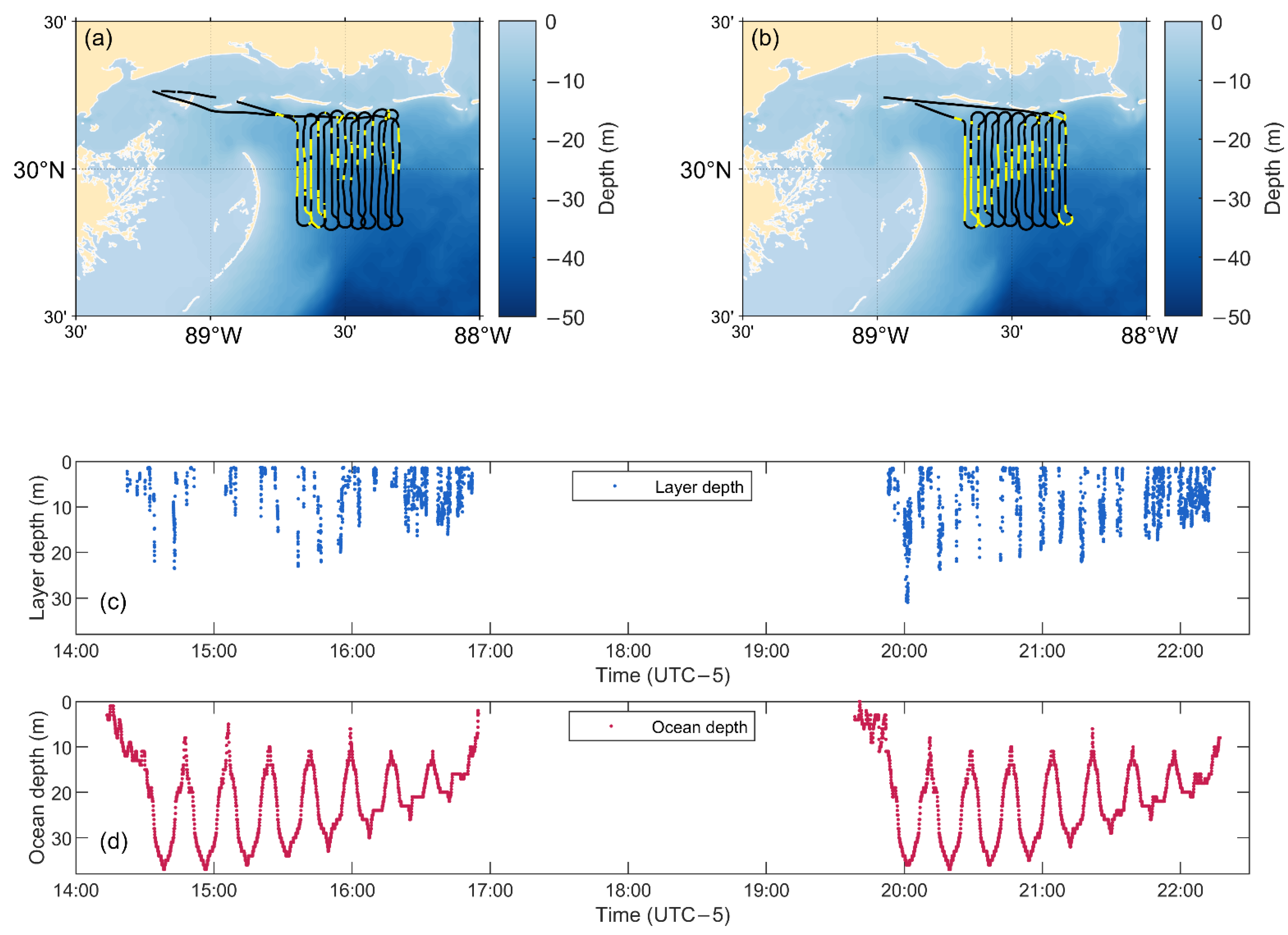
2.1. Experimental Area

The Gulf of Mexico is southeast of the North American continent and is the marginal sea of the Atlantic Ocean, with a sea area of 1,507,639 square kilometers, an average depth of 1615 m, and a maximum depth of 4400 m. The shape of the Gulf of Mexico is a semicircle, with about one third being a deep basin, one third the slope, and the rest a flat continental rim with a depth less than 200 m [19]. The Gulf of Mexico has strong northerly cold winds in winter. Tropical storms are more frequent in the summer. The Gulf of Mexico is frequently hit by hurricanes, peaking around September [20]. Phytoplankton are widespread in the Gulf of Mexico. The Gulf of Mexico has a large deep water area, but primary production is concentrated in the shallower bays, accounting for 70% of the total [21], and the carbon fixation in the Gulf of Mexico is largely controlled by the margin. Nitrogen and phosphorus are closely related to phytoplankton growth. The main source of nitrogen and phosphorus in the northern Gulf of Mexico is the Mississippi River and its tributaries, which provide 62% and 88% of terrestrial nitrogen and phosphorus sources. As the population grows, large amounts of trash and industrial wastewater are discharged into the Gulf of Mexico. In 2010, an oil spill from the Deepwater Horizon well damaged the Gulf of Mexico ecosystem, harming nearly 2100 km of shoreline and a wide range of coastal habitats [22].

During late September and early October 2011, NOAA conducted flight surveys of zooplankton, phytoplankton and fish by airborne lidar in the northern Gulf of Mexico from 87°W to 90.5°W and 28°N to 30°N. The flight route is shown as the black line in Figure 1. The lidar was mounted on a KingAir 90 twin-engine aircraft with a nominal altitude of 300 m and a flight speed of 80–100 m/s [13]. NOAA Chemical Sciences Laboratory provided the raw LIDAR data.

2.2. Lidar Data Processing

The NOAA lidar system is called FLOE (Fish Lidar, Oceanic, Experimental). It uses a Q-tuned, frequency-doubled Nd: YAG laser that emits green polarized light at a wavelength of 532 nm with a laser pulse length of about 12 ns. The penetration depth of the lidar can reach more than 30 m in offshore waters, 20–30 m on the shelf, and less than 20 m in the Mississippi River plume, with a depth resolution of 11 cm in the water [23].

The perturbation method, which assumes that the lidar attenuation coefficient is constant and ignores its variation component with depth [24,25], is utilized here to obtain characteristics of the thin layers. The depth corresponding to the maximum value of the photocathode current $I_m(z)$ was taken as the ocean surface, and the logarithm of the photocathode current was fitted to the depth by linear regression to estimate the background signal

$$I_B(z)=I_B(0)\exp (-2\alpha z)$$

(1)

where z is the depth and α is the lidar attenuation coefficient. The depth range for the regression fit was from the ocean surface to the depth at which the photocathode current was 50 dB lower than the surface value. The signal from the layer was obtained by subtracting the background signal and adjusting for background attenuation

$$I_L(z)=[I_m(\mathrm{z})-I_B(z)]\exp (2\alpha z)$$

(2)

the layer depth and thickness were calculated from the depth of the maximum value of $I_L(z)$ and its full width at half maximum. According to the existing bio-optical model [26], the background backscattering coefficient ${\beta }_B$ can be estimated from the attenuation coefficient α. The ratio of $I_m(z)$ to $I_B(z)$ is defined as the intensity $S$, and the corresponding volume backscattering coefficient ${\beta }_L=S{\beta }_B$.

This method estimates the background signal by considering the thin layer as a perturbation to the background signal. When the signal does not meet the requirements of a 50 dB drop in shallower positions, it is necessary to combine the water depth data and apply the bottom as the lower limit of the regression range.

3. Results

3.1. Data Processing

The processing of the lidar data is shown in Figure 2. In this example, one lidar echo signal is processed by fitting the photocathode current $I_m(z)$ to obtain the background signal $I_B(z)$ from 0 m to 22 m depth. The layer depth and thickness from this example are 14.6 m and 3.5 m, respectively. Since the perturbation method ignores the inhomogeneous scattering attenuation, this method will underestimate the layer signal, because the fitted background signal will be affected by the layer and slightly higher. However, the variation of the attenuation coefficient is relatively small, which will not have a substantial effect on the results.

The retrieved backscattering coefficients are shown as a three-dimensional plot on the route in Figure 3, from which the distribution of the layers can be visualized. Numerous areas of strong scattering were found on 24 September 2011. Similar thin layer structures were detected near 29°N, 88°W, and 88.5°W, suggesting a possible distribution of thin layers up to 40 km long. A larger number of thin phytoplankton layers were also detected in the latitude line of 30°N, where the depth of the seafloor varies rapidly. Since the water depth under some of the detection routes is less than 10 m, the scattering peak at the bottom are caused by the seafloor.

Figure 4 shows the results on 24 September and 4 October 2011. A thin layer extends about 5 km horizontally near 28°30′N, 87°30′W in deep water, as shown in Figure 4a,b. It is a typical pelagic layer with no contact with the seafloor. The corresponding layer depth varies as shown by the blue curves in Figure 4b, between 15 and 30 m, while the thickness is represented by the red lines, which are all less than 5 m. Figure 4c shows the results near 30°N, 88°20′W with a water depth of approximately 20 m on 4 October 2011. This thin layer extends over 4 km, with larger backscatter coefficients than that on 24 September. The strong scattering part near 0 m in Figure 4a is caused by the ocean surface, and the red part below 20 m in Figure 4c is the seafloor. Combined with the ocean depth data, the layer depth and thickness are obtained in the range from 1 m below the surface to 1 m above the seafloor, avoiding the error of identifying the ocean surface or seafloor as a layer. Note that the coordinate scales are not the same.

3.2. Occurrence Probability of Thin Layers

The location information of layers is obtained from the lidar data according to the methods in Section 2.2, which is displayed on the seawater depth map as in Figure 5a and on the monthly average sea surface chlorophyll concentration map as in Figure 5b. Scattered thin layers were discovered in areas with very deep seawater and very low chlorophyll concentrations. Dense thin layers were found in inshore areas north of 29°N, where depths were less than 1000 m and chlorophyll concentrations were over 1 mg m⁻³. These areas are around the Mississippi Delta and it is possible that the Mississippi River plume provides enough nutrients for phytoplankton. However, only a small number of thin layers were found in Chandeleur Sound. Although chlorophyll concentrations are high in Chandeleur Sound, water depths are less than 10 m, making it difficult to form nutrient concentration stratification and to evolve into thin layers [27].

The formation of thin layers is related to surface chlorophyll concentration. We calculated the probability of thin layers forming at different sea surface chlorophyll concentrations and various ocean depths, as shown in Figure 6. Chlorophyll concentrations in seawater greater than 1 mg m⁻³ can be considered as high concentrations [28], and the occurrence probability of phytoplankton thin layers in the Gulf of Mexico was highest at about 2 mg m⁻³.

The in situ growth [29] mechanism can provide some explanation for this phenomenon: light is more abundant at the surface of seawater, while nutrients containing elements such as nitrogen and phosphorus are more abundant in deep water; when both nutrient and light levels are satisfied at a certain depth, a thin layer is formed. Chlorophyll concentration is generally positively correlated with nutrient concentration. When the chlorophyll concentration is less than 1 mg m⁻³, it indicates that there is a nutrient deficiency in the water column and the phytoplankton population is low. Therefore, the probability of forming a highly aggregated thin layer in the ocean subsurface is also low. When the surface chlorophyll concentration is high (about 2 mg m⁻³), the subsurface water is rich enough in nutrients to form a large number of thin layers, so the probability is highest here.

As the chlorophyll concentration continued to increase, the probability of detecting a thin layer decreased instead, and no thin layer was found when it was greater than 6 mg m⁻³. In areas where surface chlorophyll concentration exceeded 6 mg m⁻³, the nutrient content of the sea surface is sufficiently high that it may lead to large aggregations of phytoplankton, forming surface thin layers or even algal blooms that absorbed a larger fraction of light [30]. However, the aggregation of phytoplankton on the surface is not regarded as a thin layer. As a result, the light level underwater is inadequate for the formation of thin layers. Another possible reason is the absence of nutrient concentration gradients in seawater, which is one of the conditions for the formation of thin layers. Moreover, the low total number of detections in the high chlorophyll concentration region may also make the results inaccurate.

The relationship between the occurrence probability of thin phytoplankton layer and water depth was not significant. The detection was mainly concentrated in the area of water depth less than 500 m, and the probability was higher in this range. The penetration depth of lidar was limited to about 40 m, and only the subsurface phytoplankton could be detected, while layers in deep water were missed. There is a peak near 900 m water depth in Figure 6b, corresponding to the vicinity of 29°N, 88.5°W in Figure 5a. Since the ocean depth here changes rapidly from 100 m to 1000 m, thin layers may migrate from shallow waters by currents or swimming, with randomness in direction [31], so this result has some occasionality. The lidar signal at the seawater surface is substantially enhanced due to the reflection from the air-water interface, and the presence of oceanic breaking waves makes it difficult to distinguish thin layers within 2 m depth from the signal [32]. Due to the strong waves affecting the optical properties of seawater [33], some shallow thin layers may be missed or destroyed.

3.3. Depth and Thickness of Thin Layer

The joint probability distribution of layer depth and thickness is shown in Figure 7. The depth and thickness of the thin layer in the northern Gulf of Mexico showed a normal distribution, respectively. The thickness varies from 1 m to 6 m, but is mainly concentrated within 4 m, and the depth is mainly distributed in 10–15 m. Ryan et al. detected thin layers in areas of Monterey Bay where the depth was less than 500 m in summer. Monterey Bay is the largest open bay on the west coast of the United States and is located in the central California Current System with abundant seasonal wind-driven upwelling, which is similar to the Gulf of Mexico. The vertical thickness of the thin layers ranged from 1–5 m and the depth from 12–33 m [34]. Johnston et al. obtained similar results in a larger area of Monterey Bay [35].

The detection area was divided into patches according to latitude and longitude, and the average layer depth and thickness within each patch were calculated, as shown in Figure 8. From nearshore to offshore, the color patches of layer depth change from blue to red gradually. Instead, the pattern of change in thickness is the reverse. The depth of the thin layer was shallower in the nearshore area, with an average depth of 11.5 ± 4.8 m, while the average depth in the deep area was 16.9 ± 7.75 m. The average thickness of the thin layer in the shallow water area is 3.5 ± 1.7 m, while in the deep area it is 3.0 ± 1.6 m.

Mixed layer depth (MLD) data are available from the Estimating the Circulation and Climate of the Ocean (ECCO) database [36]. In late September and early October, the MLD in the Gulf of Mexico was about 30 m [37]. According to ECCO data, in 2011 the MLD was less than 35 m in the detection area, as shown in Figure 9a. The mixed layer is a surface layer characterized by uniform to near-uniform density [38], and below the mixed layer is the pycnocline whose density increases rapidly with depth. The thin layer in the Gulf of Mexico mostly forms at the bottom of the mixed layer, which is closely related to the rich nutrients below it, as shown in Figure 9b. The correlation coefficient between MLD and thin layer depth was 0.72. In a study by Dekshenieks [39], 71% of the thin layers were found to be directly related to the pycnocline. Another factor in the formation of thin layers is the shear of the ocean currents. Due to the influence of the internal waves of the ocean, the water velocity changes rapidly with depth, and the strong lateral shear makes the phytoplankton thickness smaller and forms a thin layer with a thickness below 5 m [40]. However, due to the lack of ocean internal wave data for 2011, it is a pity that no suitable data were found for in-depth analysis.

The correlation coefficient between layer depth and ocean depth was 0.63, while only −0.11 between thickness and ocean depth, as shown in Figure 10a,b. The characteristics of the layers were also related to the chlorophyll concentration, showing that the layer depth decreased with higher chlorophyll concentration, while the thickness increased. The correlation coefficients were −0.82 and 0.36 respectively. In deeper areas of seawater, where most of the nutrients were deposited on the bottom [41], thus the thin layers were also located deeper. The high chlorophyll concentration at the sea surface indicates that the nutrient content at the surface is high enough to allow phytoplankton to grow [42], and the layer depth becomes shallower. The strong correlation between the layer depth and ocean depth and chlorophyll suggests that the layer depth is mainly controlled by the ocean topography and the distribution of nutrients in water column, consistent with the in situ mechanism. Layer thickness may be influenced by complex factors such as gyrotactic trapping, buoyancy, shear and other hydrodynamic processes [40].

High nutrient concentrations at the sea surface are also associated with eddies and upwelling. The water velocity in the eddy’s core is low, while the surrounding water velocity is high. The water pressure in the center of the eddy is greater than the surrounding area, so the water spreads around, causing a rise in nutrient salts at the bottom of the ocean in that area, leading to an increased possibility of thin layers forming around it. According to the sea surface height anomaly (SSHA), at 29°N30′, 88°W30′, there exists a central region of lower sea surface height where eddies may exist. In the research of He’s team [43], the sea surface height anomaly data in the South China Sea had been used to determine the eddies. Combined with the water flow velocity data, the presence of eddies can be confirmed, and there is another eddy with the same rotation direction on the east, as shown in Figure 11a. Upwelling caused by eddies carries nutrients to the subsurface, and this vertical exchange is more likely to form in regions with lower seawater surface temperatures in Figure 11b. Nutrients rise more easily to the surface where the sea is shallow. The combination of currents and topography contributed to the formation of the thin layer in this region.

3.4. Layer Variation in Two Detections

Two repeated detections in the same area were conducted in the afternoon and evening on Oct.4. The first measurement started at about 14:00 pm and the second measurement started at about 19:30 pm, each lasting about 3 h. The aircraft made intensive flights from the east to the west in both detections, and widespread thin layers were found as shown in Figure 12a,b. Thin layers were detected in 12% of the lidar pulses in the first measurement, and 21% in the second measurement, suggesting that more thin layers were detected at night. In a study by Li [44], the phytoplankton abundance was at a low level in the afternoon and increased rapidly from 18:00 onwards. Light is considered to be the key driver of this change.

The same repetitive variation in the layer depth was observed in both detections, indicating that it is the same thin layer which lasted for at least 8 h. The depths of the thin layer during detection are shown by the blue dots in Figure 12c and the corresponding water depths are shown by the red dots in Figure 12d. The average thin layer depth was 7.1 m in the first detection and 8.7 m in the second. The seafloor in the flight area is highly undulating, and the water depth varies between 10–40 m during the detection process. A rise and a fall of the red dots represent the aircraft flying over the detection area once, respectively. Along with the topographic relief, there is a similar variation in the thin layer depth. This indicates that in shallow water, the thin layer depth is mainly influenced by the water depth.

4. Discussion

Lidar is widely noted for its high efficiency in remote sensing detection and profiling capabilities among various methods. The penetration depth of lidar depends on the laser wavelength and the turbidity of the water. The lidar system in this paper emits 532 nm green light and can only penetrate to 20 m depth in some areas, which is more suitable for coastal waters. In the open ocean, a shorter wavelength of blue light is required to achieve the optimal penetration depth [45]. In the inversion algorithm, the perturbation method, the background signal is assumed to be ideally exponentially attenuated, which differs from the reality. This causes unavoidable errors in the results. The high-spectral-resolution lidar can provide richer information with higher accuracy to solve this problem, which is still under research [46,47,48]. In addition, Lidar responds to organisms such as phytoplankton, zooplankton, and fish in the ocean, but the species cannot be identified from the echo signal. Pre-measurement of large areas by lidar to provide guidance for subsequent field measurements, is an effective solution.

Our results show that lidar can effectively acquire scattering information of the ocean and identify thin phytoplankton layers from it. The occurrence probability of the layers and their characteristics were strongly correlated with the surface chlorophyll concentration, ocean depth and currents. One obvious point is that the thin layer occurs more nearshore and is shallower, which is consistent with Churnside’s conclusion [23]. These results can be useful for other phytoplankton detection programs. For example, the use of ocean color remote sensing can be combined to find those areas with a high probability of thin layers based on ocean surface chlorophyll concentrations. This will further improve the efficiency of detecting thin layers.

Most of the surveys in the Gulf of Mexico were carried out in two periods from afternoon to evening, as shown in Figure 13, and only lasted 13 days. Information of the thin layer variability over large scale time and seasonal variability is difficult to obtain. Repeated detections over months, seasons, and years are necessary. This will play a critical role in further work, such as identifying changes in phytoplankton species, predicting algal blooms, guiding fisheries development, etc. We analyze the layer’s characteristics and find that the occurrence of thin layers is consistent with in situ growth mechanism and is related to topography, eddy currents, and temperature. In fact, the formation of thin layer is a complex process related to biochemistry, physics, and oceanography. Environmental factors such as salinity, wind, internal waves, anoxia, etc., phytoplankton motility and zooplankton predation all influence the formation of thin layers, and the pattern of thin layer formation varies from region to region. The current explanation for the mechanism of thin layer formation is mostly limited to the analysis of independent factors. A summary and universal mechanism is expected to be proposed in the future. The thin phytoplankton layer is a concentrated area of intense biological activity, which attracts predation by zooplankton and subsequently affects fish activity. The relationship between these organisms has not been fully revealed.

5. Conclusions

In this paper, we analyzed the spatial distribution characteristics of the thin phytoplankton layer from NOAA measurements in the northern Gulf of Mexico and tried to provide a reasonable explanation for its formation. In the northern Gulf of Mexico, thin layers were more frequently found at chlorophyll concentrations below 6 mg m⁻³, with the highest probability of occurrence between 2–3 mg m⁻³, and the probability of occurrence decreased or even became zero at higher chlorophyll concentrations. The distribution of thin layers showed aggregation in general, more densely distributed in shallow water, with shallower depths and thicker thicknesses. In the inversion algorithm used in this paper, the lidar attenuation coefficient is considered as constant, but in fact the attenuation coefficient varies slightly with depth, and the accuracy of the inversion needs to be further improved. Measurements in the northern Gulf of Mexico have only been conducted for 13 days and some information such as diurnal and seasonal variation are missing. In the future, more large-scale, high-precision, and long-duration measurements are needed to verify our conclusions. The result will deepen our knowledge and understanding of the characteristics and formation mechanism of the thin phytoplankton layer.

References

1. Sullivan, J.M.; Donaghay, P.L.; Rines, J.E.B. Coastal thin layer dynamics: Consequences to biology and optics. Cont. Shelf Res. 2010, 30, 50–65. [Google Scholar] [CrossRef]
2. Benoit-Bird, K.J.; Moline, M.A.; Waluk, C.M.; Robbins, I.C. Integrated measurements of acoustical and optical thin layers I: Vertical scales of association. Cont. Shelf Res. 2010, 30, 17–28. [Google Scholar] [CrossRef]
3. Uitz, J.; Claustre, H.; Gentili, B.; Stramski, D. Phytoplankton class-specific primary production in the world’s oceans: Seasonal and interannual variability from satellite observations. Glob. Biogeochem. Cycles 2010, 24. [Google Scholar] [CrossRef]
4. Berdalet, E.; McManus, M.A.; Ross, O.N.; Burchard, H.; Chavez, F.P.; Jaffe, J.S.; Jenkinson, I.R.; Kudela, R.; Lips, I.; Lips, U.; et al. Understanding harmful algae in stratified systems: Review of progress and future directions. Deep Sea Res. Part II Top. Stud. Oceanogr. 2014, 101, 4–20. [Google Scholar] [CrossRef]
5. Boyce, D.G.; Lewis, M.R.; Worm, B. Global phytoplankton decline over the past century. Nature 2010, 466, 591–596. [Google Scholar] [CrossRef]
6. Wang, Y.; Yan, T.; Yu, R.; Zhang, Q.; Kong, F.; Zhou, M. Research progresses of thin phytoplankton layer in the ocean. Mar. Sci. 2020, 44, 86–95. [Google Scholar]
7. Lunven, M.; Guillaud, J.F.; Youénou, A.; Crassous, M.P.; Berric, R.; Le Gall, E.; Kérouel, R.; Labry, C.; Aminot, A. Nutrient and phytoplankton distribution in the Loire River plume (Bay of Biscay, France) resolved by a new Fine Scale Sampler. Estuar. Coast. Shelf Sci. 2005, 65, 94–108. [Google Scholar] [CrossRef]
8. Derenbach, J.B.; Astheimer, H.; Hansen, H.P.; Leach, H. Vertical Microscale Distribution of Phytoplankton in Relation to the Thermocline. Mar. Ecol. Prog. Ser. 1979, 1, 187–193. [Google Scholar] [CrossRef]
9. Twardowski, M.S.; Sullivan, J.M.; Donaghay, P.L.; Zaneveld, J.R.V. Microscale Quantification of the Absorption by Dissolved and Particulate Material in Coastal Waters with an ac-9. J. Atmos. Ocean. Technol. 1999, 16, 691–707. [Google Scholar] [CrossRef]
10. Moline, M.A.; Benoit-Bird, K.J.; Robbins, I.C.; Schroth-Miller, M.; Waluk, C.M.; Zelenke, B. Integrated measurements of acoustical and optical thin layers II: Horizontal length scales. Cont. Shelf Res. 2010, 30, 29–38. [Google Scholar] [CrossRef]
11. Prairie, J.C.; Franks, P.J.S.; Jaffe, J.S. Cryptic peaks: Invisible vertical structure in fluorescent particles revealed using a planar laser imaging fluorometer. Limnol. Oceanogr. 2010, 55, 1943–1958. [Google Scholar] [CrossRef]
12. Churnside, J.H. LIDAR detection of plankton in the ocean. In Proceedings of the 2007 IEEE International Geoscience and Remote Sensing Symposium, Barcelona, Spain, 23–28 July 2007; pp. 3174–3177. [Google Scholar] [CrossRef]
13. Churnside, J.; Wells, R.J.D.; Boswell, K.; Quinlan, J.; Marchbanks, R.; McCarty, B.; Sutton, T. Surveying the distribution and abundance of flying fishes and other epipelagics in the northern Gulf of Mexico using airborne lidar. Bull. Mar. Sci. 2017, 93, 591–609. [Google Scholar] [CrossRef]
14. Kampel, M.; Lorenzzetti, J.A.; Bentz, C.M.; Nunes, R.A.; Paranhos, R.; Rudorff, F.M.; Politano, A.T. Simultaneous measurements of chlorophyll concentration by lidar, fluorometry, above-water radiometry, and ocean color MODIS images in the southwestern Atlantic. Sensors 2009, 9, 528–541. [Google Scholar] [CrossRef] [PubMed]
15. Churnside, J.; Ostrovsky, L. Lidar observation of a strongly nonlinear internal wave train in the Gulf of Alaska. Int. J. Remote Sens. 2005, 26, 167–177. [Google Scholar] [CrossRef]
16. Churnside, J.H.; Donaghay, P.L. Thin scattering layers observed by airborne lidar. ICES J. Mar. Sci. 2009, 66, 778–789. [Google Scholar] [CrossRef]
17. Churnside, J.H.; Thorne, R.E. Comparison of airborne lidar measurements with 420 kHz echo-sounder measurements of zooplankton. Appl Opt. 2005, 44, 5504–5511. [Google Scholar] [CrossRef]
18. Liu, H.; Chen, P.; Mao, Z.; Pan, D.; He, Y. Subsurface plankton layers observed from airborne lidar in Sanya Bay, South China Sea. Opt. Express 2018, 26, 29134–29147. [Google Scholar] [CrossRef]
19. Turner, R.E.; Rabalais, N.N. The Gulf of Mexico. In World Seas: An Environmental Evaluation; Elsevier: Amsterdam, The Netherlands, 2019; pp. 445–464. [Google Scholar]
20. Conner, W.H.; Day, J.W.; Baumann, R.H.; Randall, J.M. Influence of hurricanes on coastal ecosystems along the northern Gulf of Mexico. Wetl. Ecol. Manag. 1989, 1, 45–56. [Google Scholar] [CrossRef]
21. Turner, R. Inputs and outputs of the Gulf of Mexico. In The Gulf of Mexico Large Marine Ecosystems; Wiley-Blackwell: Hoboken, NJ, USA, 1999; pp. 64–73. [Google Scholar]
22. Beyer, J.; Trannum, H.C.; Bakke, T.; Hodson, P.V.; Collier, T.K. Environmental effects of the Deepwater Horizon oil spill: A review. Mar. Pollut Bull. 2016, 110, 28–51. [Google Scholar] [CrossRef]
23. Churnside, J.H.; Marchbanks, R. Preliminary LIDAR Data Report. p. 27. Available online: https://csl.noaa.gov/groups/csl3/measurements/2011McArthurII/ (accessed on 30 November 2021).
24. Churnside, J.H.; Marchbanks, R.D. Inversion of oceanographic profiling lidars by a perturbation to a linear regression. Appl. Opt. 2017, 56, 5228–5233. [Google Scholar] [CrossRef]
25. Churnside, J.H.; Marchbanks, R.D. Subsurface plankton layers in the Arctic Ocean. Geophys. Res. Lett. 2015, 42, 4896–4902. [Google Scholar] [CrossRef]
26. Churnside, J.H.; Sullivan, J.M.; Twardowski, M.S. Lidar extinction-to-backscatter ratio of the ocean. Opt. Express 2014, 22, 18698–18706. [Google Scholar] [CrossRef]
27. Onitsuka, G.; Yoshikawa, Y.; Shikata, T.; Yufu, K.; Abe, K.; Tokunaga, T.; Kimoto, K.; Matsuno, T. Development of a thin diatom layer observed in a stratified embayment in Japan. J. Oceanogr. 2018, 74, 351–365. [Google Scholar] [CrossRef]
28. Nababan, B.; Muller-Karger, F.E.; Hu, C.; Biggs, D.C. Chlorophyll variability in the northeastern Gulf of Mexico. Int. J. Remote Sens. 2011, 32, 8373–8391. [Google Scholar] [CrossRef]
29. Brereton, A.; Noh, Y.; Raasch, S. Modelling a simple mechanism for the formation of phytoplankton thin layers using large-eddy simulation: In situ growth. Mar. Ecol. Prog. Ser. 2020, 653, 77–90. [Google Scholar] [CrossRef]
30. Anderson, D.M.; Garrison, D.J. Ecology and Oceanography of Harmful Algal Blooms; Spring: Berlin/Heidelberg, Germany, 1997. [Google Scholar]
31. Hill, N.; Häder, D.-P. A biased random walk model for the trajectories of swimming micro-organisms. J. Theor. Biol. 1997, 186, 503–526. [Google Scholar] [CrossRef]
32. Robertson, B.; Gharabaghi, B.; Hall, K. Prediction of incipient breaking wave-heights using artificial neural networks and empirical relationships. Coast. Eng. J. 2015, 57, 1550018. [Google Scholar] [CrossRef]
33. Terrill, E.J.; Melville, W.K.; Stramski, D. Bubble entrainment by breaking waves and their influence on optical scattering in the upper ocean. J. Geophys. Res. Ocean. 2001, 106, 16815–16823. [Google Scholar] [CrossRef]
34. Ryan, J.; McManus, M.; Paduan, J.; Chavez, F. Phytoplankton thin layers caused by shear in frontal zones of a coastal upwelling system. Mar. Ecol. Prog. Ser. 2008, 354, 21–34. [Google Scholar] [CrossRef]
35. Johnston, T.S.; Cheriton, O.M.; Pennington, J.T.; Chavez, F.P. Thin phytoplankton layer formation at eddies, filaments, and fronts in a coastal upwelling zone. Deep Sea Res. Part II Top. Stud. Oceanogr. 2009, 56, 246–259. [Google Scholar] [CrossRef]
36. Fukumori, I.; Wang, O.; Fenty, I.; Forget, G.; Heimbach, P.; Ponte, R. Synopsis of the ECCO Central Production Global Ocean and Sea-Ice State Estimate, Version 4 Release 4. Zenodo 2021. [Google Scholar] [CrossRef]
37. Muller-Karger, F.E.; Smith, J.P.; Werner, S.; Chen, R.; Roffer, M.; Liu, Y.; Muhling, B.; Lindo-Atichati, D.; Lamkin, J.; Cerdeira-Estrada, S.; et al. Natural variability of surface oceanographic conditions in the offshore Gulf of Mexico. Prog. Oceanogr. 2015, 134, 54–76. [Google Scholar] [CrossRef]
38. Thomson, R.E.; Fine, I.V. Estimating mixed layer depth from oceanic profile data. J. Atmos. Ocean. Technol. 2003, 20, 319–329. [Google Scholar] [CrossRef]
39. Dekshenieks, M.M.; Donaghay, P.L.; Sullivan, J.M.; Rines, J.E.B.; Osborn, T.R.; Twardowski, M.S. Temporal and spatial occurrence of thin phytoplankton layers in relation to physical processes. Mar. Ecol. Prog. Ser. 2001, 223, 61–71. [Google Scholar] [CrossRef]
40. Durham, W.M.; Stocker, R. Thin phytoplankton layers: Characteristics, mechanisms, and consequences. Ann. Rev. Mar. Sci. 2012, 4, 177–207. [Google Scholar] [CrossRef]
41. Joye, S.; MacDonald, I.; Montoya, J.P.; Peccini, M. Geophysical and geochemical signatures of Gulf of Mexico seafloor brines. Biogeosciences 2005, 2, 295–309. [Google Scholar] [CrossRef]
42. Brown, C.D.; Hoyer, M.V.; Bachmann, R.W.; Canfield Jr, D.E. Nutrient-chlorophyll relationships: An evaluation of empirical nutrient-chlorophyll models using Florida and north-temperate lake data. Can. J. Fish. Aquat. Sci. 2000, 57, 1574–1583. [Google Scholar] [CrossRef]
43. He, Z.G.; Wang, D.; Chen, J.; Hu, J. Eddy structure in South China Sea from satellite tracked surface drifting buoys and satellite remote sensing sea surface height. J. Trop. Oceanogr. 2001, 20, 27–35. [Google Scholar]
44. Li, C.; Chiang, K.P.; Laws, E.A.; Liu, X.; Chen, J.; Huang, Y.; Chen, B.; Tsai, A.Y.; Huang, B. Quasi-Antiphase Diel Patterns of Abundance and Cell Size/Biomass of Picophytoplankton in the Oligotrophic Ocean. Geophys. Res. Lett. 2022, 49, e2022GL097753. [Google Scholar] [CrossRef]
45. Liu, Q.; Liu, D.; Zhu, X.; Zhou, Y.; Le, C.; Mao, Z.; Bai, J.; Bi, D.; Chen, P.; Chen, W. Optimum wavelength of spaceborne oceanic lidar in penetration depth. J. Quant. Spectrosc. Radiat. Transf. 2020, 256, 107310. [Google Scholar] [CrossRef]
46. Zhou., Y.; Chen., Y.; Zhao., H.; Jamet., C.; Dionisi., D.; Chami., M.; Girolamo, P.D.; Churnside., J.H.; Malinka., A.; Zhao., H.; et al. Shipborne oceanic high-spectral-resolution lidar for accurate estimation of seawater depth-resolved optical properties. Light: Sci. Appl. Inpress 2022. [Google Scholar] [CrossRef]
47. Zhou, Y.; Liu, D.; Xu, P.; Liu, C.; Bai, J.; Yang, L.; Cheng, Z.; Tang, P.; Zhang, Y.; Su, L. Retrieving the seawater volume scattering function at the 180° scattering angle with a high-spectral-resolution lidar. Opt. Express 2017, 25, 11813. [Google Scholar] [CrossRef] [PubMed]
48. Liu, D.; Xu, P.; Zhou, Y.; Chen, W.; Han, B.; Zhu, X.; He, Y.; Mao, Z.; Le, C.; Chen, P. Lidar remote sensing of seawater optical properties: Experiment and Monte Carlo simulation. IEEE Trans. Geosci. Remote Sens. 2019, 57, 9489–9498. [Google Scholar] [CrossRef]
Figure 1. The flight route map for the airborne lidar detection in the northern Gulf of Mexico.
Remotesensing 14 04179 g001
Figure 2. The processing of the lidar data. (a) Logarithm of photocathode current and background signal. The solid black line is the photocathode current I m ( z ) , the dashed blue line is the background signal I B ( z ) from linear fit, and the red part represents the range of layers; (b) The signal after subtraction. The black line is the signal from the layer, and the red part represents the range of its full width at half maximum.
Remotesensing 14 04179 g002
Figure 3. The three-dimensional distribution of the backscattering coefficient of the detection route on 24 September 2011. The base map shows the chlorophyll concentration at the sea surface.
Remotesensing 14 04179 g003
Figure 4. Vertical slices of volume backscattering coefficient and the corresponding thin layer depth and thickness expressed as the blue and red lines, respectively. (a) Vertical slice of β L on 24 September; (b) Corresponding layer depth and thickness on 24 September; (c) Vertical slice of β L on 4 October; (d) Corresponding layer depth and thickness on 4 October.
Remotesensing 14 04179 g004
Figure 5. Maps of thin phytoplankton layer distribution. The solid black lines are the detection route, and the yellow lines are the positions where thin layers were detected. (a) Thin layer distribution plotted on the base map of seawater depth; (b) Thin layer distribution plotted on the base map of chlorophyll concentration.
Remotesensing 14 04179 g005
Figure 6. (a) Probability of occurrence of thin layers of phytoplankton at different sea surface chlorophyll concentrations; (b) Probability of occurrence of thin layers of phytoplankton at different ocean depths.
Remotesensing 14 04179 g006
Figure 7. Two-dimensional probability distribution of thin phytoplankton layer characteristics.
Remotesensing 14 04179 g007
Figure 8. Map of average layer depth and thickness. (a) Average depth of layers in different regions; (b) Average thickness of layers in different regions.
Remotesensing 14 04179 g008
Figure 9. Mixed layer depth and thin layer depth. (a) Daily mean mixed layer depth in the Gulf of Mexico on 29 September; (b) Statistical analysis of layer depth and mixed layer depth.
Remotesensing 14 04179 g009
Figure 10. Statistical analysis of (a) layer depth vs. ocean depth; (b) layer thickness vs. ocean depth; (c) layer depth vs. chlorophyll concentration; (d) layer thickness vs. chlorophyll concentration.
Remotesensing 14 04179 g010
Figure 11. The maps of sea surface height anomaly, currents and temperature on 4 October 2011. (a) Sea surface height anomaly and current velocity on 4 October 2011. Arrows represent water flow vectors, SSHA is distinguished by the color bar; (b) Sea Surface Temperature on 4 October 2011.
Remotesensing 14 04179 g011
Figure 12. The maps of layer distribution and layer depth variation with time in the two detections on 4 October. (a) Layer distribution of the first detection. The black line is the flight route. The yellow lines are the positions where thin layers were detected; (b) Layer distribution of the second detection. The black line is the flight route. The yellow lines are the positions where thin layers were detected; (c) Layer depth variation during both detections; (d) Ocean depth variation during both detections.
Remotesensing 14 04179 g012
Figure 13. Number of lidar pulses performed at various periods in the Gulf of Mexico.
Remotesensing 14 04179 g013
Publisher’s Note: MDPI stays neutral with regard to jurisdictional claims in published maps and institutional affiliations.