


Double-Stack Aggregation Network Using a Feature-Travel Strategy for Pansharpening


College of Computer Science and Technology, Chongqing University of Posts and Telecommunications, Chongqing 400065, China
*
Author to whom correspondence should be addressed.
Remote Sens. 2022, 14(17), 4224; https://0-doi-org.brum.beds.ac.uk/10.3390/rs14174224
Submission received: 20 July 2022
/
Revised: 24 August 2022
/
Accepted: 25 August 2022
/
Published: 27 August 2022
(This article belongs to the Special Issue 2nd Edition GeoAI: Integration of Artificial Intelligence, Machine Learning and Deep Learning with Remote Sensing)
Abstract
:Pansharpening methods based on deep learning can obtain high-quality, high-resolution multispectral images and are gradually becoming an active research topic. To combine deep learning and remote sensing domain knowledge more efficiently, we propose a double-stack aggregation network using a feature-travel strategy for pansharpening. The proposed network comprises two important designs. First, we propose a double-stack feature aggregation module that can efficiently retain useful feature information by aggregating features extracted at different levels. The module introduces a new multiscale, large-kernel convolutional block in the feature extraction stage to maintain the overall computational power while expanding the receptive field and obtaining detailed feature information. We also introduce a feature-travel strategy to effectively complement feature details on multiple scales. By resampling the source images, we use three pairs of source images at various scales as the input to the network. The feature-travel strategy lets the extracted features loop through the three scales to supplement the effective feature details. Extensive experiments on three satellite datasets show that the proposed model achieves significant improvements in both spatial and spectral quality measurements compared to state-of-the-art methods.
1. Introduction
Remote sensing images provide technical advantages, such as multiresolution, wide coverage, repeatable observation, and multispectral/hyperspectral recording. Therefore, they are widely used in urban area classification, vegetation cover monitoring, target identification, and national defence security [1,2,3]. Among remote sensing images, multiresolution images provide users with the highest resolution in both the spatial and spectral domains. However, due to the limitations of remote sensing imaging principles and the physical structure of sensors, the instantaneous fields of view of sensors can differ [4] therefore, satellites usually carry various sensors to acquire multiresolution images. For example, Earth observation satellites, such as QuickBird, WorldView-2 and, WorldView-3, carry two sensors to simultaneously capture two types of high-resolution remote sensing images: panchromatic (PAN) images with high spatial but low spectral resolution and multispectral (MS) images with high spectral but low spatial resolution (LRMS).
In practical remote sensing applications, MS images with high spatial and spectral resolution are often necessary, encouraging researchers to establish an effective method to generate such images from multiple images. The pansharpening algorithm was created to fully use the spatial information of PAN images and the spectral information of MS images.
Pansharpened images are important in remote sensing scenes and as a preprocessing step for image processing tasks, such as feature extraction, segmentation, and classification. In recent decades, researchers have proposed pansharpening algorithms in several directions, primarily classified into (1) component substitution (CS) methods [5,6,7,8], (2) multiresolution analysis (MRA) methods [9,10,11,12,13], (3) variational optimisation (VO)-based methods [14,15,16], and (4) deep learning methods.
The core idea of CS-based methods is to first project the MS image onto another space to separate the spatial structure component from the spectral information component. Then, a histogram matches the PAN image to the spatial structure component and replaces the spatial intensity component with the PAN image. Finally, a reverse projection returns the data to the original MS domain to obtain a sharpened MS image. Methods of this type include principal component analysis [5], intensity–hue–saturation transform [6], Gram–Schmidt (GS) sharpening [7], and partial replacement adaptive component substitution (PRACS) [8]. CS methods can obtain results with high spatial fidelity; however, this usually results in significant spectral distortion.
MRA-based methods retain more spectral information than CS methods. Moreover, MRA-based methods usually inject the spatial details extracted from PAN images into MS images through the MRA framework to obtain MS images with high spatial resolution. However, MRA methods suffer from spatial distortion, although they retain spectral information. Examples of such methods include smoothing filter-based intensity modulation (SFIM) [9], additive wavelet luminance scaling [10], “a-trous” wavelet transform [11], Laplace pyramid [12], and generalised Laplace pyramid [13], among others.
In contrast, VO-based methods consider PAN sharpening to be an optimisation problem. The key concept of VO methods is to establish the objective function, which is used to determine an appropriate solution among variational optimisation schemes. Furthermore, VO methods can reduce the distortion of spectral information, but the optimisation calculation is complex, and the time complexity is high. Common methods include P+XS [14] and Bayesian methods [15], and sparse representation-based [16] methods also belong to the VO category.
With the rapid development of hardware devices and machine learning, deep-learning-based models have achieved exciting results in various image processing fields, such as image super-resolution (SR), target detection, image segmentation, and other fields. In image SR, Dong et al. [17] pioneered an SR convolutional neural network (CNN) model using CNNs and obtained good results. In target detection, Ghorbanzadeh et al. [18] integrated CNN models with object-based image analysis (OBIA) capabilities to effectively support refugee/IDP (internally displaced person) camp planning and humanitarian assistance. In hazard detection, Ghorbanzadeh et al. [19] first applied fully convolutional network (FCN) algorithms, such as U-Net and ResU-Net, to freely available data and achieved high landslide detection performance. In image segmentation, Ronneberger et al. [20] proposed a U-Net architecture consisting of a contraction path and a symmetric expansion path and successfully trained deep networks.
Inspired by the SRCNN, Masi et al. [21] designed a three-layer CNN architecture to achieve pansharpening using the powerful nonlinear mapping ability of CNNs. This CNN application was the first in the field of pansharpening. Since then, pansharpening algorithms using deep learning have become a research focus. Wei et al. [22] designed a deep residual network with 11 layers to obtain rich detail information and strong nonlinear mapping ability. He et al. [23] summarised a detail-injection-based CNN model, which solved the redundant part of the network structure and enhanced interpretability. Liu et al. [24] combined the advantages of generative adversarial networks (GANs) and designed a GAN-based pansharpening algorithm called PSGAN. Fu et al. [25] borrowed the idea of feedback connection [26] to designed a two-path network with a feedback connection (TPNwFB), which refined the low-level features by feeding back the high-level features extracted from the feature extraction block to the low-level features. Xu et al. [27] designed a cross-directional and progressive network (CPNet) from the input image, which considers that most methods only take the four-fold upsampled LRMS and source PAN images as input. Wu et al. [28] proposed a new three-stage detail-injection-based network (TDPNet) that takes the difference between the PAN and MS images as input [29]. They designed a cascaded cross-scale fusion method to fully utilize the detail information on different scales, using a detail compensation mechanism to supplement details lost in the fusion process.
However, pansharpening is subject to some drawbacks, as follow: (1) in order to achieve powerful performance, many researches have added various large functional modules, making the model increasingly large in size with an increased number of parameters; (2) many proposed models do not sufficiently consider and treat the input images; and (3) some frameworks do not reach their full potential.
To improve and solve the problems mentioned above, we propose a double-stack aggregation network using a feature-travel strategy for pansharpening. By capturing detailed feature information on different scales in a round-robin manner, information loss due to upsampling on LRMS is reduced. The main contributions of this study are as follow:
- In the feature extraction stage, we propose a novel multiscale, large-kernel residual convolution block (MLRB) combining the ideas of large-kernel convolution and dilated convolution to extract more fine-grained detail information while effectively expanding the receptive field. The design of MLRB has positive significance for the subsequent feature fusion, especially with respect to preservation of spectral information.
- We propose a powerful double-stack feature aggregation module (DSFAM) to make full use of the feature details extracted at different levels. We aggregate the features extracted by the shallow and deep networks through multiple skip connections so that the final extracted features can fully retain the details extracted at each level, including spatial and spectral details.
- We propose a novel feature circumnavigation strategy to preserve as much detail as possible in response to the loss of sampling in LRMS images. We obtain source images at three scales as input by processing and constructing three network levels. The extracted features are looped at different scales by resampling. The looped features complement the information at the three scales, reduce the details lost in the input images due to resampling, and improve the final reconstruction results.
- We let each network layer learn the spatial and spectral detail information missing from the LRMS images and attach the loss function to each network layer to ensure that each feature loop can be supplemented with the correct information.
The rest of this paper is organised as follows. In Section 2, we review related work based on CNNs in other domains and summarise other pansharpening methods based on deep learning. In Section 3, we details the proposed DFS-Net, including the motivation for the proposal, network architecture design, and loss function definition. In Section, we present the experimental results and qualitatively and quantitatively compare the proposed method with other methods in different datasets. In Section 5, we discusses the validity of various network structures and the rationality of the overall framework. Finally, we summarize the work in Section 6.
2. Background and Related Work
2.1. Convolutional Neural Network
Researchers have studied three main aspects of many related vision tasks to improve CNN performance: depth, width, and cardinality [30].
In terms of depth, Simonyan and Zisserman [31] first proposed a very deep CNN (the VGG), arguing that the receptive field obtained using a small convolutional kernel multiple times is the same as that obtained using a large convolutional kernel once and that the number of parameters can be reduced. He et al. [32] proposed a residual learning framework to solve the gradient degradation problem that occurs during the training of deep networks, considerably improving the depth and accuracy of the neural network. Based on this, Huang et al. [33] proposed a densely connected network (DenseNet), connecting each layer to every other layer in a feedforward fashion, further optimising the gradient convergence problem of the network and obtaining improved results. To better employ the features in the residual framework, Liu et al. [34] proposed a residual feature aggregation network (RFANet), which aggregates multiple residual operations within a residual range for adequate feature extraction.
Regarding width, GoogLeNet [35] uses multiple convolutional kernels to extract features. GoogLeNet experiments reveal that width is another important factor for improving model performance.
Concerning cardinality, Xception [36] fully decouples GoogLeNet, proposing a deeply separable convolution and allowing each feature channel to be convolved using a separate convolution kernel. This method improves performance while reducing the number of parameters.
The receptive field size of a network model is also an important factor in improving performance. Yu and Koltun [37] proposed dilated convolution to systematically aggregate multiscale contextual information; dilated convolution supports the exponential expansion of the receptive field without the loss of resolution or coverage.
Ding et al. [38] reviewed the design of large kernels in modern CNNs. They suggested that using several large kernels instead of multiple small convolutions may be a more powerful paradigm. Large-kernel CNNs have much larger effective receptive fields than traditional CNNs but exhibit a higher shape bias than texture bias, providing a new way of thinking.
With the continuous development of deep learning, many novel and effective network models have emerged in various fields. These network models are limited to their original fields and motivate and inspire researchers in the field of pansharpening to apply novel ideas to CNN-based pansharpening work with good results.
2.2. Convolutional-Neural-Network-Based Pansharpening Algorithm
Because pansharpening can be considered a special form of SR, Masi et al. [21] borrowed the deep learning method employed in the field of image SR [17] and applied it to the field of pansharpening for the first time. Specifically, upsampled LRMS and PAN images are first concatenated in the channel direction and then fed into a CNN for nonlinear learning algorithm, resulting in a pansharpened image.
To improve the performance of CNN in pansharpening, Wei et al. [22] combined the concept of residual learning to design a deep CNN structure that further exploits the high nonlinearity of deep learning models. Moreover, He et al. [23] attributed the traditional pansharpening algorithm to a uniform detail injection context and combined the deep learning approach to design a new detail injection model. The proposed model provides a clear physical explanation and solves some problems of previous models.
Yang et al. [39] incorporated knowledge from the remote sensing domain to design a new deep network structure, PanNet, by focusing on the two objectives of spectral and spatial preservation. Resampled LRMS images are added to the network output to preserve the spectral information, and the network parameters are trained in the high-pass filtering domain instead of the image domain to maintain the spatial structure.
Inspired by dilated convolution [37], Fu et al. [40] proposed DMDNet with grouped multiscale dilated convolution, whereby the network model becomes more capable of extracting details and can preserve more spatial details. Unlike previous CNN-based methods that perform pansharpening at the pixel level, Liu et al. [41] proposed TFNet to fuse PAN and LRMS images at the feature level because both PAN and LRMS images contain spatial and spectral information.
Fu et al. [25] proposed TPNwFB with feedback connections to deliver feedback information through the structure of recurrent neural networks to take full advantage of powerful deep features with strong representation capability. Most deep-learning-based methods process PAN and LRMS images in a feedforward manner, such that the shallow level cannot obtain useful information from the deep level. The deep features continuously refine the shallow features in four time steps of feature extraction. The rich feature information provides strong support for the final network output results.
To fully process information, Xu et al. [27] proposed a cross-direction and progressive network. CPNet. Original images at different scales are obtained by resampling the source images in cross direction and used as the input for the fusion module at different stages to maximise the use of the multiscale information in the source images. In contrast, a progressive reconstruction loss training network maintains the consistency of the fusion results and the true values.
Wu et al. [28] proposed a three-stage detail injection network to preserve spatial and spectral information. First, a two-branch structure extracts details at multiple scales, employing downsampling using a maximum pooling operation to preserve as much feature information as possible. Then, a cascaded cross-scale fusion strategy employs the fine-scale fusion information as a priori knowledge for coarse-scale fusion, compensating for information lost during downsampling and preserving high-frequency details, making full use of the multiscale information extracted in the first stage. Finally, a multiscale skip connection block reconstructs the injected details, and the details lost due to resampling are supplemented by a multiscale detail compensation mechanism to increase the spatial details.
3. Proposed Network
In this section, we describe the specific structure of the DFS-Net model proposed in this paper. The network follows the traditional idea of detail injection into the context by injecting extracted information into the resampled LRMS images. Thus, this network has good physical interpretability. The network structure must only learn detail information, making network training easier and effectively alleviating any gradient disappearance and explosion that may occur during the network learning process.
Most deep-learning-based methods directly upsample LRMS images by a factor of four as network input. However, the image upsampling process can affect the quality of the original image. To retain and extract the information lost during the resampling of LRMS images and fully employ the information from the source PAN and LRMS images at different scales, we upsampled and downsampled LRMS images and PAN images, respectively, to form three pairs of input images at different scales and constructed three network layers.
For each layer of the input, a two-stem network was used to extract the features of the PAN and LRMS images. After overlaying the features extracted by the two-stem network on the channels, a powerful DSFAM fully extracts and uses the features at different levels. The extracted features are downsampled and upsampled in a three-scale network, and the feature information extracted at different scales is fused using a fully connected dense fusion network. Then, the reconstruction module reconstructs the features to match the dimensions of the LRMS images. Finally, the extracted detail information is injected into the LRMS images to obtain the fused images.
The structure of each network scale primarily consists of a two-stem network, DSFAM, fully dense fusion block, feature-travel route, and reconstruction module. Loss functions are attached to all three network scales, forcing each scale to extract the correct feature information. The fused image obtained at the PAN scale is the desired result. Figure 1 illustrates the main structure of DFS-Net.
3.1. Two-Stem Structure
Previous CNN-based pansharpening algorithms used only the PAN image as a carrier of spatial information and injected the information extracted from the PAN image into the LRMS image. However, in recent years, many studies [29,41] have revealed that both PAN and LRMS images contain certain spatial and spectral information. The PAN image contains rich spatial and spectral information unavailable in the LRMS image. For the backbone network to fully use the information from PAN and LRMS images, we set up two identical stem blocks for feature extraction of PAN and LRMS images and realised the fusion reconstruction and image recovery work of spatial and spectral information in the feature domain. In each network scale, one stem block takes the multiband LRMS image (size H×W×N) as input, and the other stem block duplicates the PAN image and concatenates it on the channels to take the multichannel PAN image (size H×W×N) as input.
Although the traditional method can achieve superior image resampling, we believe resampling the source image using the deep learning method is more consistent with the overall network architecture and retains the required detail information. Therefore, we used transpose and two-stride convolution to accomplish upsampling and downsampling of the LRMS and PAN images. To maintain the relative relationship between the ground-truth (GT) image and the PAN image, we used two-stride convolution with shared parameters for each layer for downsampling.
The detailed structure of the stem block is presented in Figure 2. Inspired by PanNet’s use of high-pass filtering, we designed a depthwise convolutional layer similar to high-pass filtering in the first layer and did not add a nonlinear activation layer. Using high-pass filtering allows the network training to move from the image domain to the high-pass filtering domain. However, the parameter design of the high-pass filter significantly affects the final result. To take full advantage of the parametric learning capability of deep learning, we used deep convolution to simulate the role of high-pass filtering with good results. After the high-pass-like filter layer, we extracted features using a convolutional layer with a convolutional kernel size of 3 × 3 and boosted the number of channels to three. Then, we used deep convolution again to extract features channel by channel. In the stem block, we used parametric rectified linear units (PReLUs) after each convolutional layer, except for the high-pass-like filtering layer.
The two-stem structure consists of two stem blocks, each consisting of a layer, a layer, and a layer. denotes a depthwise convolutional layer with a size f f convolutional kernel and n channels, denotes a normal convolutional layer with a size f f convolutional kernel and n channels, and denotes the PReLU activation function. In addition, and denote the extracted LRMS image and PAN image features, respectively; and denotes the concatenate operation.
3.2. Double-Stack Feature Aggregation Module
In deep learning, VGG [31] has demonstrated that depth is important for the network to extract features from images. Moreover, with the emergence of ResNet [32], the network is difficult to train due to the increased depth. In addition, ResNet effectively solves the problems of gradient disappearance, gradient explosion, and network degradation by adding residual connections so that the gradient can be updated more directly. Network degradation indicates that model performance temporarily bottlenecks when the network reaches a certain depth, making it difficult to increase. When the network continues to deepen, model performance on the testing set instead declines. By adding residual connections, network training becomes easier, the network depth is considerably increased, and many deeper networks are developed, opening up a new phase of deep learning.
Although network layers have become deeper, recent research has tended to ignore the features extracted at each layer, which contains important information. The features extracted by shallow-layer networks are closer to the input and contain more information about pixel points, primarily fine-grained information, such as colour, texture, edge, and corner information. A shallow network has a smaller receptive field and a smaller receptive field overlap area, so the network is guaranteed to capture more details. The features extracted by deeper networks are closer to the output. They contain more abstract information (i.e., semantic information), primarily coarse-grained information, because the receptive field increases, the overlapping area between receptive fields increases, the image information is compressed, and information about the totality of the image is obtained. In pansharpening, a shallow network extracts more pixel-level information, containing colour and edge information, and deep networks extract additional semantic information. The flexible use of each level of information helps to preserving spectral and spatial information.
Inspired by the above ideas, we propose a DSFAM that can fully employ the features at each level. As depicted in Figure 3, DSFAM consists of four continuous residual aggregation blocks (CRABs), and each CRAB contains four MLRBs, forming a double-stack aggregation structure. Finally, a 1 × 1 convolutional layer is used to weight the aggregated features and maintain the dimensionality, similar to the attention mechanism. In DSFAM, the double-stack aggregation structure is designed so that all parts of the deep network can be used effectively, and the final extracted features are very powerful. We believe that the increase in computation and number of parameters by properly adding skip connections would be less than by redesigning a new module, a classic example of which is U-Net [20]. That is, a high-performance network structure design does not always require additional modules, and fully employing the original structure of the network may be a better approach, which is one of the manifestations of high efficiency.
The CRAB structure is presented in Figure 4. We borrowed the aggregated design of classical residual blocks from RFANet [34] and repositioned the skip connections by combining the overall idea of DSFAM. In many networks, residual blocks are stacked together to form the network backbone. However, in multiple consecutive residual blocks, the features extracted from the first residual block must pass through long paths with repeated convolution and addition operations to reach the last residual block. As a result, the residual features at different levels are difficult to apply fully and play a very local role in the learning process of the whole network, which fits in with the idea of the DSFAM design.
Unlike RFANet, instead of aggregating multiple residual blocks within a residual range, we aggregated continuous residual blocks. The RFANet approach is to aggregate residual features within residual features rather than directly aggregate residual features, as displayed in Figure 5. The advantage of the continuous residual aggregation used in the CRAB is that the residual features at each level can be used more directly, whereas the skip connection at each level makes the gradient update more easily. In addition, the CRAB results from a special optimisation based on DSFAM design ideas.
In the CRAB, to enhance the receptive field of the ordinary residual block and extract features on multiple scales, we designed an MLRB instead of an ordinary convolutional block; the structure of the MLRB is depicted in Figure 6. We used four parallel branches for feature extraction to separately obtain features on different scales while maintaining computational volume. Inspired by DMDNet [40] and related studies [37], we extended the receptive field of small-scale convolutional kernels using dilated convolution to achieve feature extraction at multiple scales with different expansion coefficients.
However, some studies [38,42] have demonstrated that dilation convolution may have grid effects. Although this drawback can be overcome by mixing convolutions with different expansion coefficients, information loss still occurs on edges, and some pixels in the image are not used. Some approaches propose using a compensation mechanism to compensate for the disadvantages of dilated convolution to address this problem. The compensation mechanism generally works by extracting features using a new module, concatenating them with the features extracted by the dilated convolution on the channel, and feeding them to the next part.
However, the problem with this approach is that although the compensation mechanism compensates for drawbacks, this is achieved by increasing the number of parameters and computational effort. The idea of large-kernel networks proposed by RepLKNet [38] provides new inspiration. RepLKNet reviews the design of large kernels in CNNs. Large-kernel convolutions mostly appeared in early CNNs, such as AlexNet [43], but in most networks after VGG, the strategy of stacking multiple 3 × 3 convolutional layers was used. Large-kernel convolution is a way to increase the receptive field, which is more sensitive to shape bias compared to multiple small convolutions. Both dilated and large-kernel convolution can increase the receptive field, and whether their combination is superior is the motivation to design the MLRB.
In the MLRB, we again set up two small branches within each parallel branch to combine large-kernel and dilated convolution, solving the possible lattice effect of dilated convolution. The inputs of these two small branches are the same in the large-kernel convolutional layer (the dilated convolutional kernel can be regarded as a large kernel) and the 3 × 3 basic convolutional layer. Next, the features extracted from the two small branches are numerically summed to obtain the composite features. Finally, the composite features extracted from all parallel branches are concatenated and fused using a 1 × 1 convolutional layer.
The numerical superposition of the features extracted on the two small branches is equivalent to the convolutional operation of the input image with a composite convolutional kernel. The structure of the composite convolutional kernel in the MLRB is depicted in Figure 7, whereby we set a basic 3 × 3 convolution in each parallel branch, and each parallel branch is paired with a large-kernel convolution of varying sizes, with a 9 × 9 convolution on the leftmost side and an expansion on the right side, representing a dilated convolution with factors of 2, 3, and 4. Yellow indicates the composite part of the two convolutional kernels.
The entire DSFAM can be defined as:
where denotes the convolutional layer with a convolutional kernel size of f × f, n is the number of channels, is the PReLU activation function, denotes the MLRB blocks of the four levels in CRAB, denotes the CRAB blocks of the four levels in DSFAM, x denotes the input image of each level of CRAB, and denotes the concatenate operation.
3.3. Fully Dense Fusion Block
To fully retain the feature information extracted from each layer and effectively fuse the features on different scales, we adopted a fully dense fusion (FDF) block. The specific structure of FDF is presented in Figure 8. DenseNet was the first to employ the concept of dense connection, connecting each layer to all other layers in a feedforward manner, alleviating the gradient disappearance problem and enhancing feature propagation while reusing features. Many studies have employed the concept of dense connectivity, and pansharpening methods, such as TPNwFB and CPNet, have used dense connectivity and achieved good results.
We set up a 1 × 1 convolution at the beginning and end of the FDF to maintain the dimensionality. The basic component is a combination of 1 × 1 and 3 × 3 convolution. Considering the computational cost and experimental results, we set the number of basic components of the FDF to six. All convolutional layers of the FDF are followed by PReLU activation functions. In the framework design, the number of feature fusions at different levels is high, so the size of the FDF should not be too large. The main task of FDF is to perform the initial fusion of feature maps at different scales at the feature level to obtain improved and powerful features.
3.4. Feature-Travel Route
Fu et al. [25] proposed a new pansharpening algorithm, TPNwFB, by combining the feedback connections in SR tasks. The TPNwFB implements the feedback mechanism by passing the deep features extracted in the previous time step to the same feature extraction block in the next time step. The deep features provide more information to the shallow features and continuously refine the shallow features to obtain powerful deep features.
Xu et al. [27] extracted information from the LRMS image scale to make more use of the information on multiple scales of the input image. This method continuously passes the low-scale image information to the PAN image scale to progressively fuse PAN and MS images.
The feature-travel strategy is derived from feedback connections and progressive fusion. We also used images on three scales as input (PAN, middle, and MS scale) for the sake of description. The features first extracted at the PAN scale are cyclically fused with features extracted at other scales to enrich the missing multiscale feature information at the PAN scale. Specifically, the features extracted at the PAN scale are downsampled to the next scale for fusion as the prior information of the middle-scale features, and the process is cycled until the MS scale. After reaching the MS scale, the fused information is upsampled as a complement to the coarse-scale information in the previous layer and returns to the PAN scale. For each downsampling, the number of channels is twice as many as the original quantity. For each upsampling, the number of channels is half the original amount. The feature-travel strategy supplements the information on the three scales, reduces the details lost in the input image due to resampling, and improves the final reconstruction results.
3.5. Reconstruction Block
For fused features, we used a three-layer reconstruction block for the final reconstruction task. The structure of the reconstruction block is presented in Figure 9. We adopted a three-step strategy to consider the possible information loss problem of an excessively drastic channel dimension change during the reconstruction process. The number of channels output by each convolutional layer is half the input, and the number of channels output by the third convolutional layer is four, consistent with the number of channels of the LRMS image. Moreover, the activation function of the third convolutional layer is replaced with the tanh function to eliminate the effect of outliers. Combining the residual feature map and LRMS output from the reconstruction block provides required high-resolution multispectral (HRMS) image.
This process can be defined as:
The notation denotes the concatenate operation; denotes the convolutional layer; and f and n denote the convolutional kernel size and the number of channels, respectively. In Equation (9), In_channel represents the number of input channels; y represents the input image of the reconstruction block at each level; and and denote the tanh activation function and the PReLU activation function, respectively.
3.6. Loss Function
We chose the loss function to optimise the network parameters. Because it squares the difference, the function expands the influence of the outliers on network optimisation and obtains images that are usually smoother and have the potential for local minimisation problems. The loss function is less sensitive to outliers and can obtain more edge information. Many studies and experimental results [24,41,44] have demonstrated the superiority of the function. We attached loss functions to the network at each scale to ensure that feature travel is supplemented with valid multiscale feature information. We included three networks on the scales in one iteration, resulting in three sharpened images. The mathematical expression of the total loss function is as follows:
where and denote the ground truth images on the PAN scale and HRMS images output by the network on the PAN scale, respectively; and denote the ground-truth images on the middle scale and HRMS images output by the network on the middle scale, respectively; and denote the ground-truth images on the MS scale and HRMS images output by the network on the MS scale, respectively; and N represents the number of samples in each training batch.
4. Experiments and Analysis
In this section, we demonstrate the effectiveness and superiority of the proposed method through experiments on the QuickBird, WorldView-2, and WorldView-3 datasets. In the early experiments, the best model was selected by comparing and evaluating the training and testing results of various network parameter models. Finally, we compared the best model built using several existing algorithms to demonstrate the superiority of the proposed method.
4.1. Dataset
To evaluate the performance of the proposed double-stack aggregation network based on the feature-travel strategy, we trained and tested the model on datasets collected from three satellite sensors (Quickbird, WorldView-2, and WorldView-3). The number of bands and the spatial and radiometric resolution (RR) of the different satellite sensors are presented in Table 1.
We followed Wald’s protocol [45] to generate the reduced-resolution image dataset. The process of simulating the training dataset according to Wald’s protocol is illustrated in Figure 10. In brief, Wald’s protocol downsamples the original PAN and LRMS images by a resolution factor of four. The downsampled PAN and LRMS images are treated as the input images for the simulation experiment, whereas the original LRMS images are used as the GT images in the simulation experiment.
The dataset for each satellite was divided into training and testing sets with a different subset of the source images. The training set was used for network training, and the testing set was used to evaluate the network performance. The number of training and testing sets in different satellite datasets is listed in Table 2.
The LMS (a reduced-resolution form of MS images), MS, and (reduced-resolution form of PAN images) image sizes of the training data were 16 × 16 × 4, 64 × 64 × 4, and 64 × 64 × 1, respectively. The full-resolution MS and PAN image sizes of the testing data were 64 × 64 × 4 and 256 × 256 × 4, respectively.
4.2. Experimental Setup
The network architecture for this study was implemented using the PyTorch deep learning framework and trained on an NVIDIA RTX 3090 graphics processing unit (GPU). The training time for the whole project was about 4 hours. We used the Adam [46] optimisation algorithm to minimise the loss function and optimise the model. We set the learning rate size to 0.001, the weight decay to 10−8, and the total number of iterations to 4 × 10⁴. The image patch size was set to 64 × 64, and the batch size was set to 16. The red, green, and blue bands of the multispectral image were used as the imaging bands of the RGB image to form a colour image to facilitate visualisation, and the visualisation results were given using ENVI. All image bands were simultaneously used to calculate the image evaluation index. The CNN-based experiments were completed on a GPU, and CS/MRA-based experiments were completed on a central processing unit (CPU) using MATLAB to compare the pansharpening effect.
4.3. Evaluation Indicators
We compared the performance of different algorithms using two types of experiments: a simulated experiment concerning HRMS images and a real experiment without reference to HRMS images because they often lack actual application scenarios for remote sensing images. To more objectively evaluate and analyse the performance of algorithms according to various aspects of different datasets, we selected the following objective evaluation metrics based on the characteristics of simulated and real experiments:
- Spectral angle mapper (SAM) [47]: The SAM measures the spectral aberration of the pansharpened image and reference image, defined as the angle between the spectral vector after pansharpening and the reference image within the same pixel, which is calculated as follows:where and are two spectral vectors. In addition, the SAM averages over all images to generate a global measure of spectral distortion. For an ideal pansharpened image, the SAM should be set to 0.
- Correlation coefficient (CC) [41]: The CC is another widely used measure of the spectral quality of pansharpened images. The CC between the pansharpened image (X) and the corresponding reference image (Y) is calculated as follows:where w and h are the width and height of the image, and denotes the average value of the image. The CC value ranges from −1 to +1, with an ideal value of +1.
- Quality index (Q4) [48]: The Q4 is a four-band extension of the Q index and is defined as follows:where and are two quaternions consisting of the spectral vector of the MS image (i.e., z = a + ib + jc + kd), where and are the means of and , respectively; is the covariance of and ; and and are the variances of and , respectively. The ideal value of Q4 is 1.
- Relative average spectral error (RASE): The RASE estimates the overall spectral quality of the PAN sharpened image, where RMSE(Bi) is the root mean square error of the i band of the pansharpened image and the reference image, and M is the mean value of the N bands:
- Erreur relative globale adimensionnelle de synthèse (ERGAS) [49]: The ERGAS, also known as the relative global dimensional synthesis error, is a commonly used global quality index expressed as:where h and l are the spatial resolutions of PAN and MS images, respectively; RMSE(Bi) is the root mean square error of the ith band of the fused image and reference image; and M(Bi) is the average of the original MS band (Bi). The ideal value of ERGAS is 0.
- Structural similarity index measure (SSIM) [50]: The SSIM is the similarity measure between two images, defined as follows:where x and y are the pansharpened and reference images, respectively; and are the mean and variance of the corresponding images, respectively; is the covariance between the fused and reference images; and and are constants used to maintain stability. The ideal value of SSIM is 1.
- Quality with no reference (QNR) [51]: The QNR is an evaluation index used to evaluate the reference-free image and consists of and , where represents the degree of spectral distortion, mathematically expressed as:where UIQI represents the universal image quality evaluation index; and are b-band and c-band low-spatial-resolution MS images, respectively; and are b-band and c-band pansharpened images, respectively; and p is a positive integer of the magnification difference. The representation of UIQI is:where x and y indicate the original and test images, respectively; denotes the covariance between x and y images; and are the mean and variance of x, respectively; and and are the mean and variance of y, respectively.
Furthermore, denotes the degree of spatial distortion, mathematically expressed as:
where and denote the PAN image and reduced-resolution version of the PAN image, respectively; and q is a positive integer of the amplification difference. The QNR is expressed as:
where and are constants. The optimal value of QNR is 1, and the ideal value for and is 0.
4.4. Simulated and Real Experiments
Simulated and real experiments were conducted on different datasets to verify the effectiveness and reliability of the network. Representative traditional and deep-learning-based algorithms were selected from three datasets to compare the performance of various methods using subjective visual and objective metrics. The selected traditional algorithms are CS-based methods, such as PRACS [8] and GS [7]. Among the MRA-based methods, DWT [52], HPF [53], GLP [13], SFIM [9], and IND [54] were considered. We selected four deep-learning-based methods for comparison: DMDNet [40], CPNet [27], TPNwFB [25], and TDPNet [28].
4.4.1. Experiment with the Quickbird Dataset
The fusion results using the QuickBird dataset are presented in Figure 11. Figure 11a–c depicts the reference, PAN, and LRMS images, respectively, Figure 11d–j presents the fusion results of the conventional algorithm, and Figure 11k–o represents the fusion results of the deep learning methods.
Subjective analysis of all fused images and comparison of methods shows that the fused images of non-deep learning methods differ significantly in terms of colour and detail compared to the reference images, which is a typical physical distortion phenomenon in traditional methods (i.e., spectral distortion and spatial distortion). Among these methods, the fused image of DWT is the worst, with severe spectral and spatial distortion and obvious artefacts. The fused image of IND also suffers from spectral distortion, although the spatial detail is better preserved than for DWT. The fused image of PRACS is relatively better in terms of spatial detail, but there is obvious spectral distortion, and the overall tone does not match the original image. The fused images of HPF, GLP, and SFIM present with the same physical distortion. Moreover, GLP and SFIM do not differ significantly in terms of the subjective effect of the fused images, which are better than the previous methods but with obvious artefacts on the edges. The subjective effect of the GS-fused images is the best among the traditional methods.
All selected deep learning methods have good fidelity in spectral and spatial terms. A closer examination reveals that DFS-Net performs better in terms of spectral details than other deep learning algorithms. The selected deep learning methods are all relatively representative and high-quality algorithms; thus, it is difficult to determine differences in texture details from a subjective perspective. We used evaluation metrics to compare the differences between the algorithms to further assess the strengths and weaknesses of each method from an objective perspective. Table 3 presents the objective results of each method according to various evaluation metrics.
DMDNet uses 10 convolutional layers to extract the detail information. Although the performance is improved using null convolution, the use of null convolution is very limited, and the overall number of parameters is small, which is the worst among all deep learning methods.
CPNet, through the innovation of the framework, is the most effective algorithm in terms of volume, and TDPNet strengthens the application of deep learning, further increasing the volume and improving the overall performance relative to CPNet. The spatial details and spectral information are closer to the reference image.
TPNwFB uses feedback connections to achieve pansharpening, with the highest volume among the listed methods. It outperforms all methods except DFS-Net in terms of metrics.
The proposed method achieves significantly better performance than all methods in terms of spectral difference, global error, and SSIM. This outcome proves the effectiveness of the proposed method.
4.4.2. Experiments with the Worldview-2 Dataset
The fusion results using the WorldView-2 dataset are presented in Figure 12. In Figure 12a–c illustrates the reference, PAN, and LRMS images, respectively, Figure 12d–j displays the fusion results of traditional algorithms, and Figure 12k–o provides the fusion results of deep learning methods.
The figure visualises the significant colour differences of the conventional method compared to the reference image, suffering from more severe spatial blurring than the deep learning method. The LRMS images used in the simulation experiments contain spectral information not present in the reference image (i.e., blue pixel points in the zoomed-in region), which is caused by multiple resamplings of the images. All fused images generated by the traditional methods exhibit spectral distortion at the corresponding positions. In contrast, the deep learning methods do exhibit spectral distortion, indicating that they are more robust than the traditional methods. Among the deep-learning-based methods, the fusion results of DFS-Net have indicate a significant advantage relative to other methods in terms of spectral preservation compared with the reference image, and some edge details in buildings are more obvious than in the other methods.
The results of each method according to different objective evaluation metrics are listed in Table 4. The difference in metric values between the methods on the WorldView-2 dataset is not as considerable as on the QuickBird dataset, but the fused images generated by the deep learning methods still perform considerably better than those generated by the traditional methods according to all metrics.
As previously observed, the GS method is the best performer among the traditional methods, followed by the PRACS method. The GS method with the best performance among the traditional methods still has a small gap compared to the method with the worst metric values among the deep learning methods.
Regarding the deep learning methods, DMDNet extracts the detail information in the high-pass image domain, which is likely to lose more details; thus, it is somewhat inferior to the other methods in terms of the SSIM and global error. The advantage of the deep learning method on the WorldView-2 dataset is not as obvious due to the dataset’s characteristics, whereby the convergence of the network model is difficult. However, the proposed method still presents the best results for all metrics, and the model performance is the best for spatial details and spectral information fidelity.
4.4.3. Experiment with the WorldView-3 Dataset
The fusion results using the WorldView-3 dataset are presented in Figure 13. Figure 13a–c displays the reference, PAN, and LRMS images, respectively, Figure 13d–j presents the fusion results of the traditional algorithm, and Figure 13k–o provides the fusion results of the deep learning method.
In the traditional method, the fusion image generated by DWT still suffers from spectral distortion, with numerous obvious artefacts, making the whole image appear blurry. The fusion image generated by IND has better spatial details than DWT but still exhibits obvious spectral distortion. The best performers are still the GS and PRACS methods, with distinct spatial edges, especially for buildings, but they suffer from the same spectral distortion visible to the naked eye. The differences between the deep learning methods become are reduced but still exhibit better spatial and spectral fidelity than the traditional methods.
To further compare the performance of each method, we analysed the networks using an objective evaluation method. The results for each method according to the objective evaluation metrics are listed in Table 5. All methods perform better on the WorldView-3 dataset according to the metrics.
Among the traditional methods, GS and PRACS are very close to the deep learning methods in terms of SAM, CC, and Q4 metrics, implying good results from the perspective of spectral information preservation. However, a large gap exists between these two methods and the deep learning methods in SSIM and ERGAS metrics, indicating that some problems still occur in preserving spatial detail information in the traditional methods.
Among the CNN-based methods, CPNet exhibits outstanding performance in terms of the Q_AVE and SSIM metrics, indicating the significance of using the multiscale information of the input image for spatial information preservation. In addition, TPNwFB achieves the best performance in terms of the SAM, ERGAS, and CC metrics, indicating the advantage of a feedback connection with respect to the overall image quality and the preservation of spectral information. The performance of TDPNet is the same as that of TPNwFB. The proposed network obtained the most competitive results in preserving spectral information and spatial information mining compared to all selected comparison methods. Based on all objective evaluation metrics, the proposed method significantly outperforms existing fusion methods, proving the effectiveness of the method.
4.4.4. Experiments with Quickbird Real Datasets
We used the trained model from the simulation experiments and original images as input to generate the fused images in real experiments. The real experiments directly input the original MS and PAN images into the model without image resampling to ensure ideal full-resolution experimental results, and the other models followed a similar approach.
The fusion results using the QuickBird real dataset are illustrated in Figure 14. Figure 14a,b shows the upsampled LRMS and PAN images, respectively (resolution, 256 × 256 pixels), Figure 14c–i presents the fusion results of the conventional algorithm, and Figure 14j–n depicts the fusion results of the deep learning methods. Table 6 lists the results of the objective analysis of each method according to the index values.
The fused images generated by DWT and GS present with obvious spectral distortion. The DWT images are duller, and the GS images are more vivid than images generated with other methods. The PRACS method achieves the most balanced performance of all traditional methods, with no obvious spatial distortion of the buildings and backgrounds and a more realistic colour perception relative to other traditional methods. No significant difference in terms of perception was observed between the deep learning methods. The proposed method is more sensitive to small areas, such as the white dots on the top of the house in the zoomed-in area. The proposed method is the clearest and brightest, and the image content is smoother than other methods.
The GS method has the worst Ds metrics due to its frequency domain conversion, which means most spatial information is lost. As PRACS is an MRA-based method, its metrics are superior. Its Ds metrics are also better than all other traditional methods, indicating that PRACS maintains the advantages of the MRA method (i.e., improved preservation of spectral and spatial information).
The metrics are also close for the deep learning methods. The TDPNet and TPNwFB achieve similar results, and TPNwFB is slightly better than TDPNet in terms of the Ds metrics, whereas TDPNet is better in terms of the metrics. In addition, TPNwFB achieves a global optimum in spatial preservation (i.e., the Ds metric) due to the feedback connections. The proposed method is also very close to TPNeFB in terms of the Ds metric and ranks second globally. Because the proposed method uses a more powerful feature reuse and feature extraction module, it achieves the best result in terms of the metric, which fully illustrates that the spectral information is derived from LRMS images and contained in PAN images. Considering these three metrics, the proposed network achieves better results in the full-resolution experiments, proving that the ideas and innovations presented herein positively contribute to the field of pansharpening.
4.4.5. Generalization to New Satellites
Our network, although trained on a relatively small number of datasets, still performs well across satellite data sources and with generalisability. To demonstrate this, we trained our model and other DL methods on the Quickbird satellite dataset and tested it on the WorldView-3 satellite dataset. The visual results are shown in Figure 15. CPNet and TPNwFB show relatively poor detail, whereas DMDNet and our model are better at preserving edge detail. The objective metric results are shown in Table 7, and as in the previous judgement, DMDNet outperforms the other methods in most categories, whereas our model achieves superior results relative to DMDNet in terms of the objective metrics. This indicates that our model is robust on new satellite images and that the proposed multiscale module can cope with intersatellite differences better than DMDNet. Based on the experiments conducted across satellite datasets, we are very confident that our approach is not only generalisable but also that the test results on the same satellite dataset are very reliable.
4.4.6. Model Efficiency Evaluation
We used the performance time, model size, number of parameters, and floating-point operations per second (FLOPs) to comprehensively evaluate the selected deep learning model. Table 8 shows that this approach is smaller than TPNwFB and TDPNet in terms of model size and number of parameters. The proposed model employs a feature-travel strategy on three scales; thus, the FLOPs are slightly higher, and the running time is longer than for TDPNet; however, the FLOPs and performance time are much smaller than for TPNwFB, which uses feedback connections, resulting in FLOPs several times higher than for other methods. In other words, the proposed method performs best and exhibits a degree of improvement in metrics, such as execution time and the number of parameters, compared to other high-performance methods, proving that this method is very efficient.
5. Discussion
In this section, we investigate the role of each model part through ablation experiments to demonstrate the effectiveness of each module. Here, we focus on the influence of the DSFAM and feature-travel strategy, and the following discussion is based on the experimental results with the QuickBird data.
5.1. Discussion of DSFAM
The DSFAM is designed to extract feature information in a comprehensive and detailed manner, primarily consisting of double-stack aggregated skip connections, CRAB, and MLRB. The MLRB extracts information at different scales by expanding the receptive field, and the CRAB and double-stack aggregated skip connections fully obtain features extracted at different levels by reusing features. To verify the effectiveness of DSFAM, we conducted experiments on the QuickBird dataset, comparing the double-stack aggregated skip connections, CRAB, and MLRB included in DSFAM.
First, we conducted ablation experiments on the large-kernel convolutional part of the MLRB. We added large-kernel convolution to the 3 × 3 convolution and dilated convolution for feature compounding; thus, the size design for the large-kernel convolution must be verified. We also added the original dilated convolutional combination without multiscale convolution as a supplementary comparison.
Table 9 details the performance of the model under various combinations. The base part is a 3×3 convolution. The experiments reveal that the best performance can be obtained when the size of the large-kernel and dilated convolutions are the same. The effect of using the dilated convolution alone is much worse than that of the MLRB, proving that the overall design is very effective. We also tested a 31 × 31 size convolution recommended in RepLKNet; it significantly improved the pansharpening task but reduced the effect, possibly as a result of the difference between the classification and fusion tasks.
To verify the effectiveness of the double-stack aggregated skip connections and CRAB, we individually compared each layer of skip connections and added the original RFANet architecture as a supplementary comparison. The objective evaluation metrics are listed in Table 10. The “no_first_layer” method indicates the elimination of the outermost aggregated skip connections. “Origin_Resnet” indicates the replacement of the CRAB with the original ResNet structure (i.e., the elimination of the inner aggregated jump connection), and “using_RFA” indicates the replacement of the structure of the CRAB with the structure used by RFANet. The metrics reveal that the modified continuous residual aggregation block significantly improved relative to the RFANet structure, indicating that the proposed design is more efficient than RFANet. Tests on each layer of aggregated skip connections reveal that all connections are essential, and the outermost connection is even more important than the inner connection. The comparative experimental results for each DSFAM module prove that the entire proposed DSFAM module is very effective in improving the overall performance of the network.
5.2. Discussion of the Feature-Travel Strategy
To effectively acquire and supplement the feature information at each scale, we designed a feature-travel strategy to enhance the already extracted feature details. We set up two sets of comparison experiments for demonstration. “Only_pan_scale” indicates that no three-pair multiscale input is used, and only the PAN and MS images are used as input (i.e., only the PAN-scale construction in the original structure). “Progressive” indicates that the features are only fed from the low scale to the high scale without a loop process. A comparison of the objective evaluation indices is provided in Figure 16.
The objective evaluation metrics reveal the effect of using the feature-travel strategy. Both SAM and SSIM metrics achieved encouraging results compared to the other two comparison experiments, indicating that the feature-travel strategy has a positive effect on the preservation of spectral and spatial information and proving its effectiveness and rationality. Further analysis of these two comparison experiments revealed a surprising fact. The network using the progressive fusion structure is less effective than the PAN-scale network, which is more concise, whereas the number of parameters and computational effort of the former network are far greater than the latter. This outcome demonstrates that blindly stacking convolutional layers or adding convolutional blocks can affect the final fusion results, also motivating the pursuit of high efficiency. Correct a priori knowledge can help to avoid problems and build new efficient algorithms, in line with the original intention of the design of DFS-Net.
6. Conclusions
To efficiently preserve the spectral and spatial information of the input images, we propose a double-stack aggregation network using a feature-travel strategy for pansharpening. The method incorporates the concept of detail injection into the design of the overall framework to reduce the difficulty of network training using three pairs of source images at different scales as inputs to complement the information of the input images at these scales.
We designed a DSFAM to fully employ the features extracted at different levels and introduced a new multiscale large-kernel convolution block to expand the convolutional field of perception and extract effective features from finer levels. We propose a novel feature circulation strategy to circularly complement the features extracted at the three scales to more effectively use and complement the information from different image scales. The features at various levels are upsampled and downsampled for the initial fusion in the network at various scales, effectively linking the three scales and generating powerful fused features that improve the final image reconstruction results.
Extensive experiments and analyses on the WorldVIew-2, WorldVIew-3, and QuickBird datasets demonstrate that DFS-Net preserves the spectral and spatial information and obtains more detailed fusion results better than other methods, especially for the sections with a large amount of edge information, such as buildings, traffic paths, and vegetation. With respect to model efficiency, DFS-Net achieves better performance with lower cost than other comparative methods, improving the efficiency of existing algorithms and proving the potential value of the method.
The relatively small number of images used for training is one of the limitations of the present study due to the publicly available data used in our dataset. Furthermore, the number of parameters of our model, although less than some more recent methods, is still relatively large and has the potential impact the fusion performance. We will address these limitations in future research.
Author Contributions
Data curation, W.L.; formal analysis, W.L.; methodology, W.L. and M.H.; validation, M.H.; visualization, M.H. and M.X.; writing—original draft, M.H.; writing—review and editing, M.H. and M.X. All authors have read and agreed to the published version of the manuscript.
Funding
This research was funded by the National Natural Science Foundation of China (nos. 61972060 and 62027827), the National Key Research and Development Program of China (no. 2019YFE0110800), the Natural Science Foundation of Chongqing (cstc2020jcyj- zdxmX0025 and cstc2019cxcyljrc-td0270).
Data Availability Statement
Data sharing is not applicable to this article.
Acknowledgments
The authors would like to thank all the reviewers for their valuable contributions to our work.
Conflicts of Interest
The authors declare no conflict of interest.
References
- Yilmaz, C.S.; Yilmaz, V.; Gungor, O. A theoretical and practical survey of image fusion methods for multispectral pansharpening. Inf. Fusion 2022, 79, 1–43. [Google Scholar] [CrossRef]
- Du, P.J.; Xia, J.S.; Zhang, W.; Tan, K.; Liu, Y.; Liu, S.C. Multiple Classifier System for Remote Sensing Image Classification: A Review. Sensors 2012, 12, 4764–4792. [Google Scholar] [CrossRef]
- Xie, Y.C.; Sha, Z.Y.; Yu, M. Remote sensing imagery in vegetation mapping: A review. J. Plant Ecol. 2008, 1, 9–23. [Google Scholar] [CrossRef]
- Ghassemian, H. A review of remote sensing image fusion methods. Inf. Fusion 2016, 32, 75–89. [Google Scholar] [CrossRef]
- Chavez, P.S.; Kwarteng, A.Y. Extracting spectral contrast in landsat thematic mapper image data using selective principal component analysis. Photogramm. Eng. Remote Sens. 1989, 55, 339–348. [Google Scholar]
- Huang, P.S.; Tu, T.M. A new look at IHS-like image fusion methods (vol 2, pg 177, 2001). Inf. Fusion 2007, 8, 217–218. [Google Scholar] [CrossRef]
- Laben, C.A.; Brower, B.V. Process for Enhancing the Spatial Resolution of Multispectral Imagery Using Pan-Sharpening. U.S. Patent 6,011,875, 4 January 2000. [Google Scholar]
- Choi, J.; Yu, K.; Kim, Y. A New Adaptive Component-Substitution-Based Satellite Image Fusion by Using Partial Replacement. Ieee Trans. Geosci. Remote Sens. 2011, 49, 295–309. [Google Scholar] [CrossRef]
- Liu, J.G. Smoothing Filter-based Intensity Modulation: A spectral preserve image fusion technique for improving spatial details. Int. J. Remote Sens. 2000, 21, 3461–3472. [Google Scholar] [CrossRef]
- Otazu, X.; Gonzalez-Audicana, M.; Fors, O.; Nunez, J. Introduction of sensor spectral response into image fusion methods. application to wavelet-based methods. Ieee Trans. Geosci. Remote Sens. 2005, 43, 2376–2385. [Google Scholar] [CrossRef]
- Shensa, M.J. The discrete wavelet Transform-Wedding the a trous and mallat algorithms. Ieee Trans. Signal Processing 1992, 40, 2464–2482. [Google Scholar] [CrossRef]
- Burt, P.J.; Adelson, E.H. The laplacian pyramid as a compact image code. Ieee Trans. Commun. 1983, 31, 532–540. [Google Scholar] [CrossRef]
- Aiazzi, B.; Alparone, L.; Baronti, S.; Garzelli, A. Context-driven fusion of high spatial and spectral resolution images based on oversampled multiresolution analysis. Ieee Trans. Geosci. Remote Sens. 2002, 40, 2300–2312. [Google Scholar] [CrossRef]
- Ballester, C.; Caselles, V.; Igual, L.; Verdera, J.; Rouge, B. A variational model for P+XS image fusion. Int. J. Comput. Vis. 2006, 69, 43–58. [Google Scholar] [CrossRef]
- Fasbender, D.; Radoux, J.; Bogaert, P. Bayesian data fusion for adaptable image pansharpening. Ieee Trans. Geosci. Remote Sens. 2008, 46, 1847–1857. [Google Scholar] [CrossRef]
- Li, S.T.; Yang, B. A New Pan-Sharpening Method Using a Compressed Sensing Technique. Ieee Trans. Geosci. Remote Sens. 2011, 49, 738–746. [Google Scholar] [CrossRef]
- Dong, C.; Loy, C.C.; He, K.M.; Tang, X.O. Image Super-Resolution Using Deep Convolutional Networks. Ieee Trans. Pattern Anal. Mach. Intell. 2016, 38, 295–307. [Google Scholar] [CrossRef]
- Ghorbanzadeh, O.; Tiede, D.; Wendt, L.; Sudmanns, M.; Lang, S.F. Transferable instance segmentation of dwellings in a refugee camp-integrating CNN and OBIA. Eur. J. Remote Sens. 2021, 54, 127–140. [Google Scholar] [CrossRef]
- Ghorbanzadeh, O.; Crivellari, A.; Ghamisi, P.; Shahabi, H.; Blaschke, T. A comprehensive transferability evaluation of U-Net and ResU-Net for landslide detection from Sentinel-2 data (case study areas from Taiwan, China, and Japan). Sci. Rep. 2021, 11, 20. [Google Scholar] [CrossRef]
- Ronneberger, O.; Fischer, P.; Brox, T. U-Net: Convolutional Networks for Biomedical Image Segmentation. In Proceedings of the 18th International Conference on Medical Image Computing and Computer-Assisted Intervention (MICCAI), Munich, Germany, 5–9 October 2015; pp. 234–241. [Google Scholar]
- Masi, G.; Cozzolino, D.; Verdoliva, L.; Scarpa, G. Pansharpening by Convolutional Neural Networks. Remote Sens. 2016, 8, 22. [Google Scholar] [CrossRef]
- Wei, Y.C.; Yuan, Q.Q.; Shen, H.F.; Zhang, L.P. Boosting the Accuracy of Multispectral Image Pansharpening by Learning a Deep Residual Network. Ieee Geosci. Remote Sens. Lett. 2017, 14, 1795–1799. [Google Scholar] [CrossRef]
- He, L.; Rao, Y.Z.; Li, J.; Chanussot, J.; Plaza, A.; Zhu, J.W.; Li, B. Pansharpening via Detail Injection Based Convolutional Neural Networks. Ieee J. Sel. Top. Appl. Earth Obs. Remote Sens. 2019, 12, 1188–1204. [Google Scholar] [CrossRef] [Green Version]
- Liu, Q.J.; Zhou, H.Y.; Xu, Q.Z.; Liu, X.Y.; Wang, Y.H. PSGAN: A Generative Adversarial Network for Remote Sensing Image Pan-Sharpening. Ieee Trans. Geosci. Remote Sens. 2021, 59, 10227–10242. [Google Scholar] [CrossRef]
- Fu, S.P.; Meng, W.H.; Jeon, G.; Chehri, A.; Zhang, R.Z.; Yang, X.M. Two-Path Network with Feedback Connections for Pan-Sharpening in Remote Sensing. Remote Sens. 2020, 12, 16. [Google Scholar] [CrossRef]
- Li, Z.; Yang, J.L.; Liu, Z.; Yang, X.M.; Jeon, G.; Wu, W.; Soc, I.C. Feedback Network for Image Super-Resolution. In Proceedings of the 32nd IEEE/CVF Conference on Computer Vision and Pattern Recognition (CVPR), Long Beach, CA, USA, 16–20 June 2019; pp. 3862–3871. [Google Scholar]
- Xu, H.; Le, Z.L.; Huang, J.; Ma, J.Y. A Cross-Direction and Progressive Network for Pan-Sharpening. Remote Sens. 2021, 13, 25. [Google Scholar] [CrossRef]
- Wu, Y.; Feng, S.; Lin, C.; Zhou, H.; Huang, M. A Three Stages Detail Injection Network for Remote Sensing Images Pansharpening. Remote Sens. 2022, 14, 1077. [Google Scholar] [CrossRef]
- Deng, L.J.; Vivone, G.; Jin, C.; Chanussot, J. Detail Injection-Based Deep Convolutional Neural Networks for Pansharpening. Ieee Trans. Geosci. Remote Sens. 2021, 59, 6995–7010. [Google Scholar] [CrossRef]
- Woo, S.H.; Park, J.; Lee, J.Y.; Kweon, I.S. CBAM: Convolutional Block Attention Module. In Proceedings of the 15th European Conference on Computer Vision (ECCV), Munich, Germany, 8–14 September 2018; pp. 3–19. [Google Scholar]
- Simonyan, K.; Zisserman, A. Very Deep Convolutional Networks for Large-Scale Image Recognition. arXiv 2014, arXiv:1409.1556. [Google Scholar]
- He, K.M.; Zhang, X.Y.; Ren, S.Q.; Sun, J.; Ieee. Deep Residual Learning for Image Recognition. In Proceedings of the 2016 IEEE Conference on Computer Vision and Pattern Recognition (CVPR), Seattle, WA, USA, 27–30 June 2016; pp. 770–778. [Google Scholar]
- Huang, G.; Liu, Z.; van der Maaten, L.; Weinberger, K.Q.; Ieee. Densely Connected Convolutional Networks. In Proceedings of the 30th IEEE/CVF Conference on Computer Vision and Pattern Recognition (CVPR), Honolulu, HI, USA, 21–26 July 2017; pp. 2261–2269. [Google Scholar]
- Liu, J.; Zhang, W.J.; Tang, Y.T.; Tang, J.; Wu, G.S.; Ieee. Residual Feature Aggregation Network for Image Super-Resolution. In Proceedings of the IEEE/CVF Conference on Computer Vision and Pattern Recognition (CVPR), Seattle, WA, USA, 14–19 June 2020; pp. 2356–2365. [Google Scholar]
- Szegedy, C.; Liu, W.; Jia, Y.Q.; Sermanet, P.; Reed, S.; Anguelov, D.; Erhan, D.; Vanhoucke, V.; Rabinovich, A.; Ieee. Going Deeper with Convolutions. In Proceedings of the IEEE Conference on Computer Vision and Pattern Recognition (CVPR), Boston, MA, USA, 7–12 June 2015; pp. 1–9. [Google Scholar]
- Chollet, F.; Ieee. Xception: Deep Learning with Depthwise Separable Convolutions. In Proceedings of the 30th IEEE/CVF Conference on Computer Vision and Pattern Recognition (CVPR), Honolulu, HI, USA, 21–26 July 2017; pp. 1800–1807. [Google Scholar]
- Yu, F.; Koltun, V. Multi-Scale Context Aggregation by Dilated Convolutions. arXiv 2015, arXiv:1511.07122. [Google Scholar]
- Ding, X.; Zhang, X.; Zhou, Y.; Han, J.; Ding, G.; Sun, J. Scaling Up Your Kernels to 31 × 31: Revisiting Large Kernel Design in CNNs. arXiv 2022, arXiv:2203.06717. [Google Scholar]
- Yang, J.F.; Fu, X.Y.; Hu, Y.W.; Huang, Y.; Ding, X.H.; Paisley, J.; Ieee. PanNet: A deep network architecture for pan-sharpening. In Proceedings of the 16th IEEE International Conference on Computer Vision (ICCV), Venice, Italy, 22–29 October 2017; pp. 1753–1761. [Google Scholar]
- Fu, X.Y.; Wang, W.; Huang, Y.; Ding, X.H.; Paisley, J. Deep Multiscale Detail Networks for Multiband Spectral Image Sharpening. Ieee Trans. Neural Netw. Learn. Syst. 2021, 32, 2090–2104. [Google Scholar] [CrossRef]
- Liu, X.Y.; Liu, Q.J.; Wang, Y.H. Remote sensing image fusion based on two-stream fusion network. Inf. Fusion 2020, 55, 1–15. [Google Scholar] [CrossRef]
- Wang, P.Q.; Chen, P.F.; Yuan, Y.; Liu, D.; Huang, Z.H.; Hou, X.D.; Cottrell, G.; Ieee. Understanding Convolution for Semantic Segmentation. In Proceedings of the 18th IEEE Winter Conference on Applications of Computer Vision (WACV), Lake Tahoe, NV, USA, 12–15 March 2018; pp. 1451–1460. [Google Scholar]
- Krizhevsky, A.; Sutskever, I.; Hinton, G.E. ImageNet Classification with Deep Convolutional Neural Networks. Commun. ACM 2017, 60, 84–90. [Google Scholar] [CrossRef]
- Shao, Z.M.; Lu, Z.X.; Ran, M.S.; Fang, L.Y.; Zhou, J.L.; Zhang, Y. Residual Encoder-Decoder Conditional Generative Adversarial Network for Pansharpening. IEEE Geosci. Remote Sens. Lett. 2020, 17, 1573–1577. [Google Scholar] [CrossRef]
- Wald, L.; Ranchin, T.; Mangolini, M. Fusion of satellite images of different spatial resolutions: Assessing the quality of resulting images. Photogramm. Eng. Remote Sens. 1997, 63, 691–699. [Google Scholar]
- Kingma, D.; Ba, J. Adam: A Method for Stochastic Optimization. arXiv 2014, arXiv:1412.6980. [Google Scholar]
- Yuhas, R.H.; Goetz, A.F.H.; Boardman, J.W. Discrimination among semi-arid landscape endmembers using the Spectral Angle Mapper (SAM) algorithm. In Proceedings of the Summaries of the Third Annual JPL Airborne Geoscience Workshop, Pasadena, CA, USA, 1–5 June 1992; pp. 147–149. [Google Scholar]
- Alparone, L.; Baronti, S.; Garzelli, A.; Nencini, F. A Global Quality Measurement of Pan-Sharpened Multispectral Imagery. IEEE Geosci. Remote Sens. Lett. 2004, 1, 313–317. [Google Scholar] [CrossRef]
- Wald, L. Quality of high resolution synthesised images: Is there a simple criterion? In Proceedings of the Third Conference "Fusion of Earth Data: Merging Point Measurements, Raster Maps and Remotely Sensed Images", Sophia Antipolis, France, 26 January 2000; pp. 99–103. [Google Scholar]
- Zhou, W.; Bovik, A.C.; Sheikh, H.R.; Simoncelli, E.P. Image quality assessment: From error visibility to structural similarity. IEEE Trans. Image Process. 2004, 13, 600–612. [Google Scholar]
- Alparone, L.; Alazzi, B.; Baronti, S.; Garzelli, A.; Nencini, F.; Selva, M. Multispectral and panchromatic data fusion assessment without reference. Photogramm. Eng. Remote Sens. 2008, 74, 193–200. [Google Scholar] [CrossRef]
- Zhou, J.; Civco, D.L.; Silander, J.A. A wavelet transform method to merge Landsat TM and SPOT panchromatic data. Int. J. Remote Sens. 1998, 19, 743–757. [Google Scholar] [CrossRef]
- Schowengerdt, R.A. Reconstruction of multispatial, multispectral image data using spatial frequency content. Photogramm. Eng. Remote Sens. 1980, 46, 1325–1334. [Google Scholar]
- Khan, M.M.; Chanussot, J.; Condat, L.; Montanvert, A. Indusion: Fusion of Multispectral and Panchromatic Images Using the Induction Scaling Technique. Geosci. Remote Sens. Lett. IEEE 2008, 5, 98–102. [Google Scholar] [CrossRef] [Green Version]
Figure 1.
Detailed structure of the proposed double-stack aggregation network using the feature-travel strategy. Gold colour represents the input images (PAN and LRMS images).
Figure 1.
Detailed structure of the proposed double-stack aggregation network using the feature-travel strategy. Gold colour represents the input images (PAN and LRMS images).

Figure 2.
Detailed structure of the stem block; d denotes depthwise convolution.

Figure 3.
Detailed structure diagram of a double-stack feature aggregation module (DSFAM).

Figure 4.
Detailed structure diagram of continuous residual aggregation block (CRAB).

Figure 5.
Detailed structure diagram of the residual feature aggregation framework (RFANet).

Figure 6.
Detailed structure diagram of multiscale large-kernel residual convolution block (MLRB).

Figure 7.
Composite convolutional kernel structure diagram: (a) construction in the multiscale large-kernel residual convolution block (MLRB) (orange indicates the composite part of the two convolutional kernels) and (b) the regular dilated structure.
Figure 7.
Composite convolutional kernel structure diagram: (a) construction in the multiscale large-kernel residual convolution block (MLRB) (orange indicates the composite part of the two convolutional kernels) and (b) the regular dilated structure.

Figure 8.
Fully dense fusion (FDF) block structure diagram; numbers in parentheses indicate the number of channels output by FDF at the PAN, middle, and MS scales.
Figure 8.
Fully dense fusion (FDF) block structure diagram; numbers in parentheses indicate the number of channels output by FDF at the PAN, middle, and MS scales.

Figure 9.
Detailed structure of the reconstruction block.

Figure 10.
The process of generating a training dataset according to Wald’s protocol. The data represented by the red text are used for simulated experiments, whereas the data represented by the black text are used for real experiments.
Figure 10.
The process of generating a training dataset according to Wald’s protocol. The data represented by the red text are used for simulated experiments, whereas the data represented by the black text are used for real experiments.

Figure 11.
Results for four bands using the QuickBird dataset (resolution, 256 × 256 pixels): (a) reference image; (b) PAN; (c) LRMS; (d) DWT; (e) HPF; (f) GS; (g) GLP; (h) SFIM; (i) IND; (j) PRACS; (k) DMDNet; (l) CPNet; (m) TPNwFB; (n) TDPNet; (o) ours algorithm.
Figure 11.
Results for four bands using the QuickBird dataset (resolution, 256 × 256 pixels): (a) reference image; (b) PAN; (c) LRMS; (d) DWT; (e) HPF; (f) GS; (g) GLP; (h) SFIM; (i) IND; (j) PRACS; (k) DMDNet; (l) CPNet; (m) TPNwFB; (n) TDPNet; (o) ours algorithm.

Figure 12.
Results for four bands using the WorldView-2 dataset (resolution, 256 × 256 pixels): (a) reference image; (b) PAN; (c) LRMS; (d) DWT; (e) HPF; (f) GS; (g) GLP; (h) SFIM; (i) IND; (j) PRACS; (k) DMDNet; (l) CPNet; (m) TPNwFB; (n) TDPNet; (o) our algorithm.
Figure 12.
Results for four bands using the WorldView-2 dataset (resolution, 256 × 256 pixels): (a) reference image; (b) PAN; (c) LRMS; (d) DWT; (e) HPF; (f) GS; (g) GLP; (h) SFIM; (i) IND; (j) PRACS; (k) DMDNet; (l) CPNet; (m) TPNwFB; (n) TDPNet; (o) our algorithm.

Figure 13.
Results for four bands using the WorldView-3 dataset (resolution, 256 × 256 pixels): (a) reference image; (b) PAN; (c) LRMS; (d) DWT; (e) HPF; (f) GS; (g) GLP; (h) SFIM; (i) IND; (j) PRACS; (k) DMDNet; (l) CPNet; (m) TPNwFB; (n) TDPNet; (o) ours algorithm.
Figure 13.
Results for four bands using the WorldView-3 dataset (resolution, 256 × 256 pixels): (a) reference image; (b) PAN; (c) LRMS; (d) DWT; (e) HPF; (f) GS; (g) GLP; (h) SFIM; (i) IND; (j) PRACS; (k) DMDNet; (l) CPNet; (m) TPNwFB; (n) TDPNet; (o) ours algorithm.

Figure 14.
Results for four bands using the QuickBird real dataset (resolution, 256 × 256 pixels): (a) upsampled LRMS; (b) PAN; (c) DWT; (d) HPF; (e) GS; (f) GLP; (g) SFIM; (h) IND; (i) PRACS; (j) DMDNet; (k) CPNet; (l) TPNwFB; (m) TDPNet; (n) ours algorithm.
Figure 14.
Results for four bands using the QuickBird real dataset (resolution, 256 × 256 pixels): (a) upsampled LRMS; (b) PAN; (c) DWT; (d) HPF; (e) GS; (f) GLP; (g) SFIM; (h) IND; (i) PRACS; (j) DMDNet; (k) CPNet; (l) TPNwFB; (m) TDPNet; (n) ours algorithm.

Figure 15.
Network generalisation capabilities tested on WorldView3 ((d–h) are trained on QuickBird). (a) Reference image; (b) PAN; (c) LRMS; (d) DMDNet; (e) CPNet; (f) TPNwFB; (g) TDPNet; (h) our algorithm.
Figure 15.
Network generalisation capabilities tested on WorldView3 ((d–h) are trained on QuickBird). (a) Reference image; (b) PAN; (c) LRMS; (d) DMDNet; (e) CPNet; (f) TPNwFB; (g) TDPNet; (h) our algorithm.

Figure 16.
The effect of the feature-travel route on the result of pansharpening fusion.


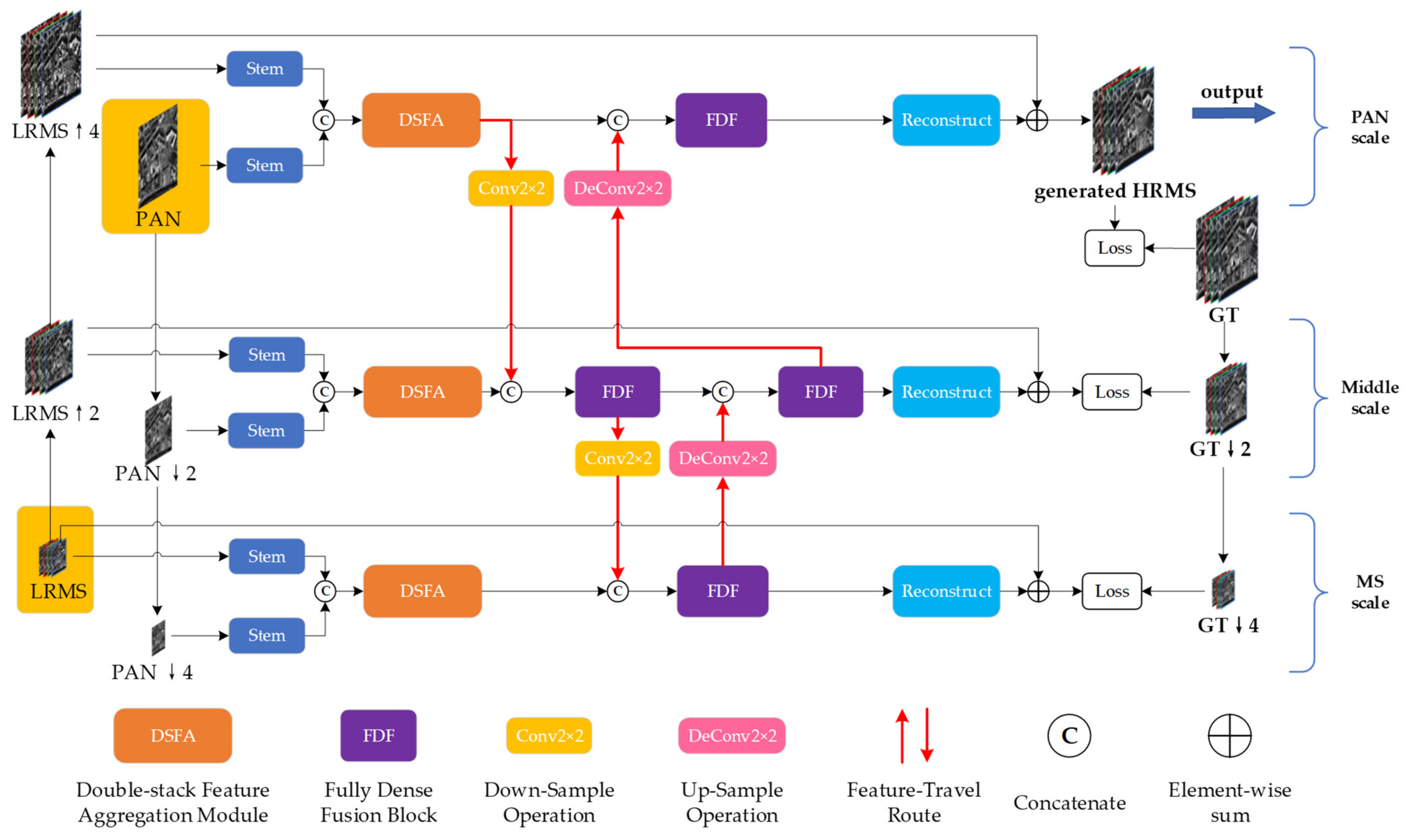
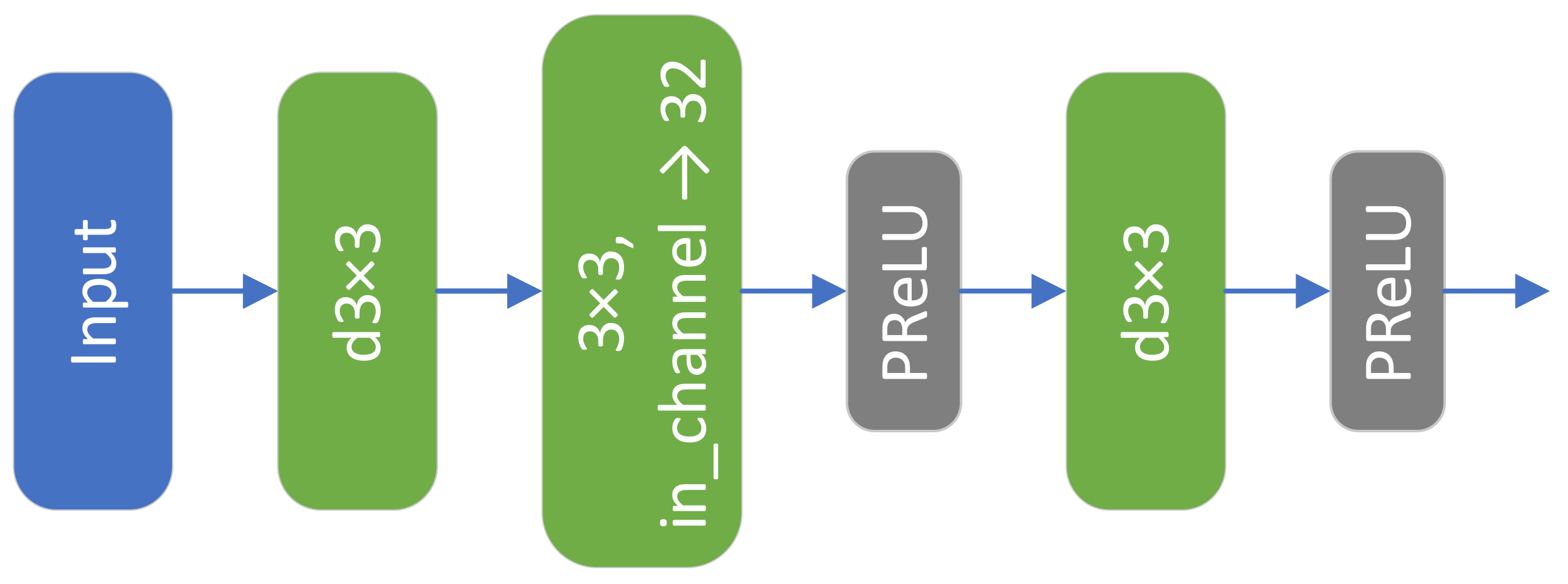
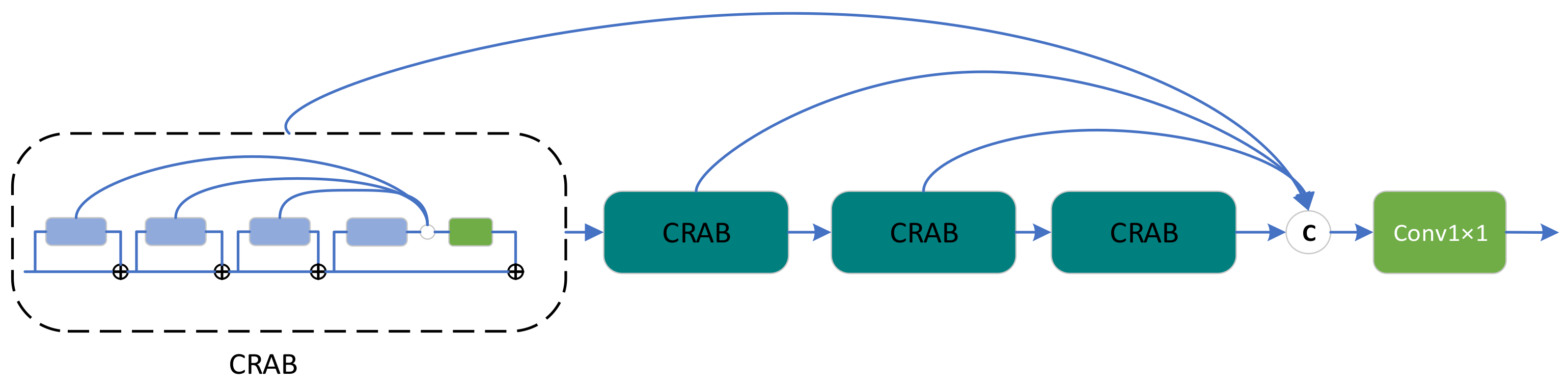
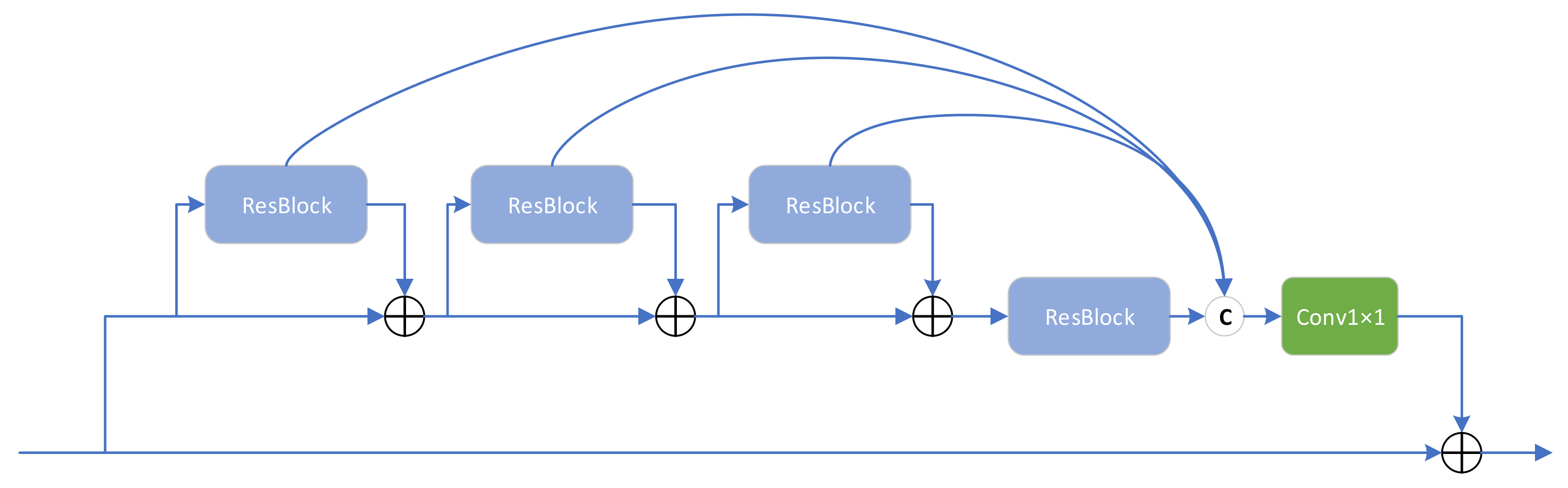
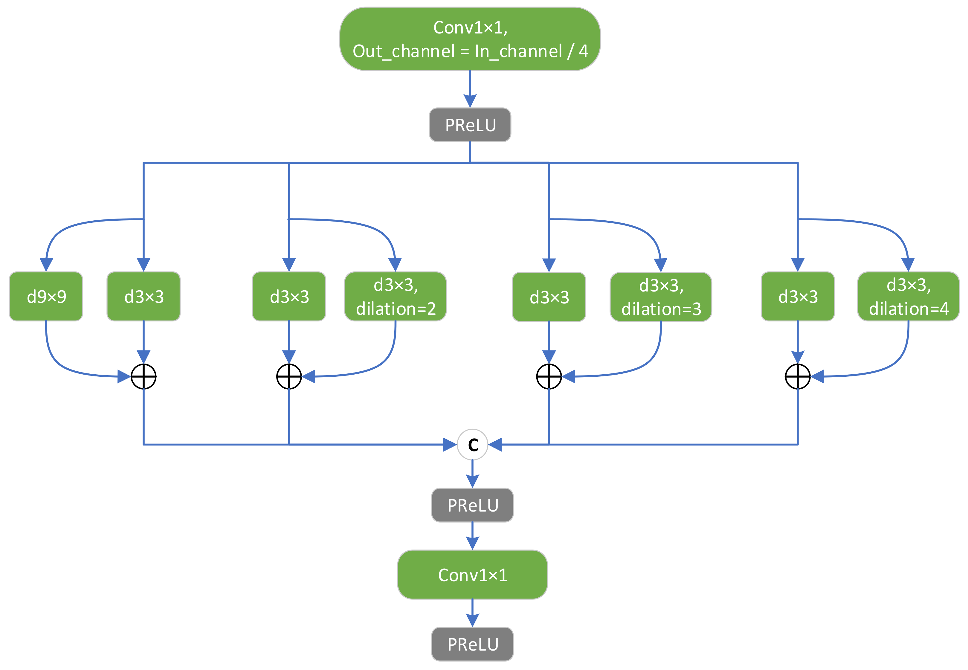
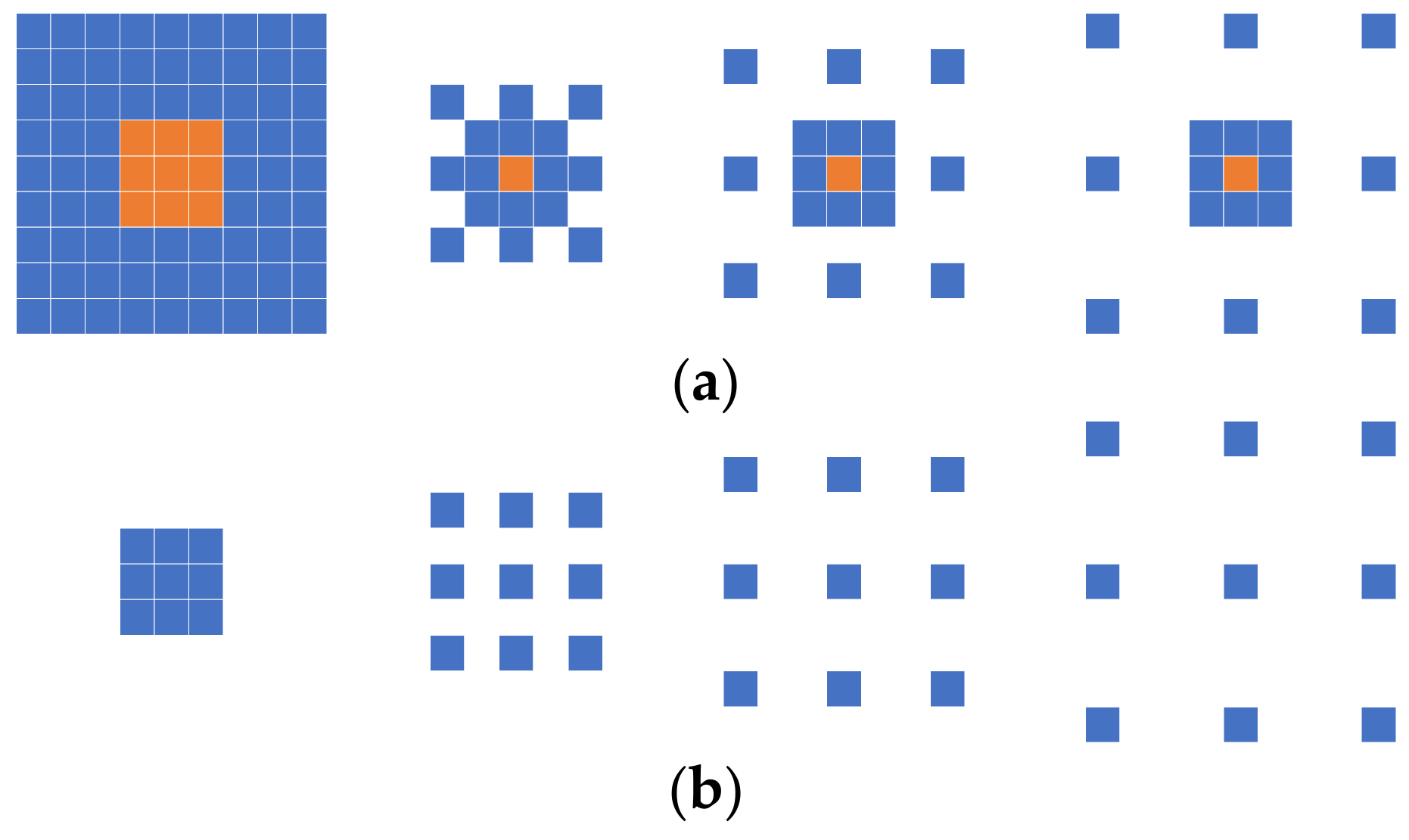
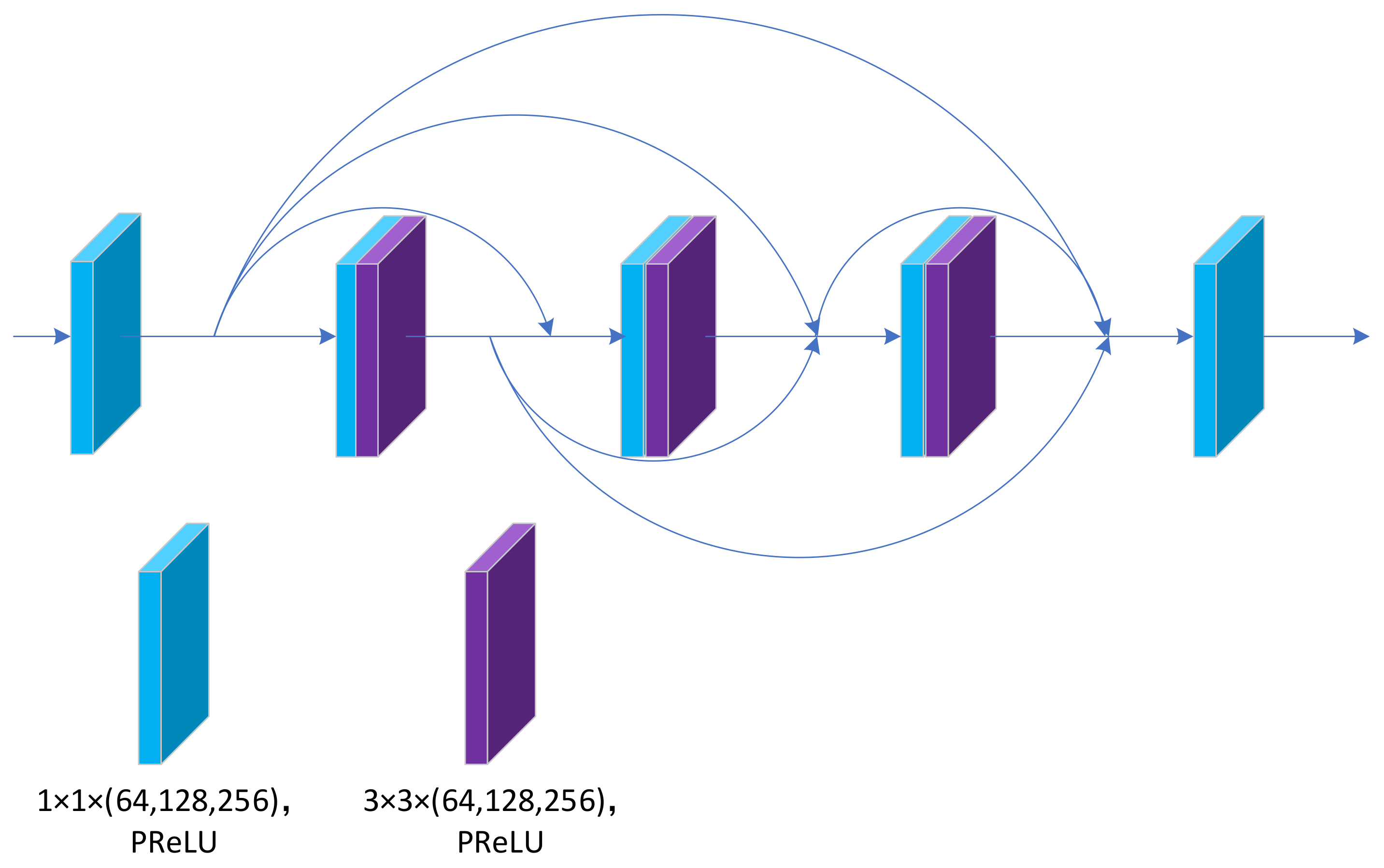
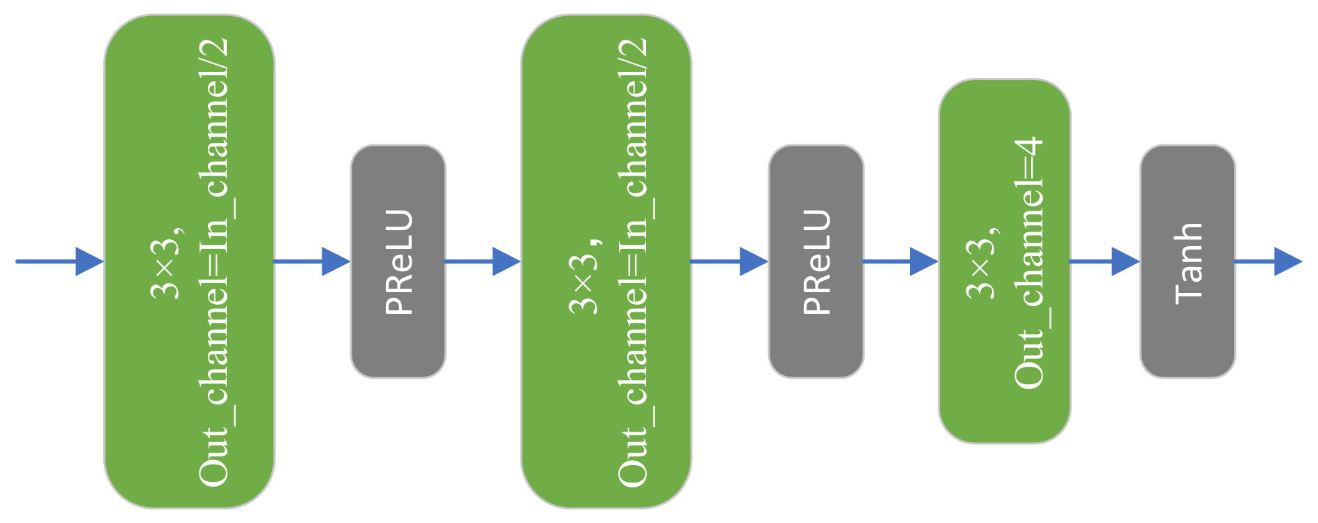
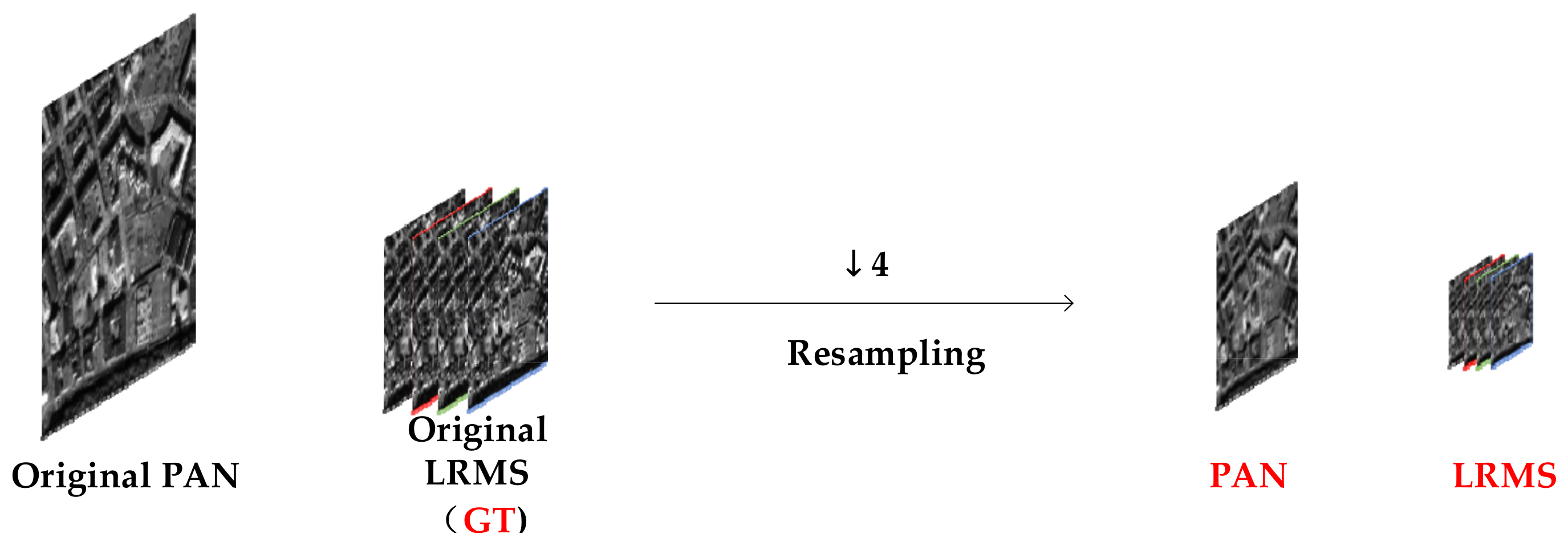
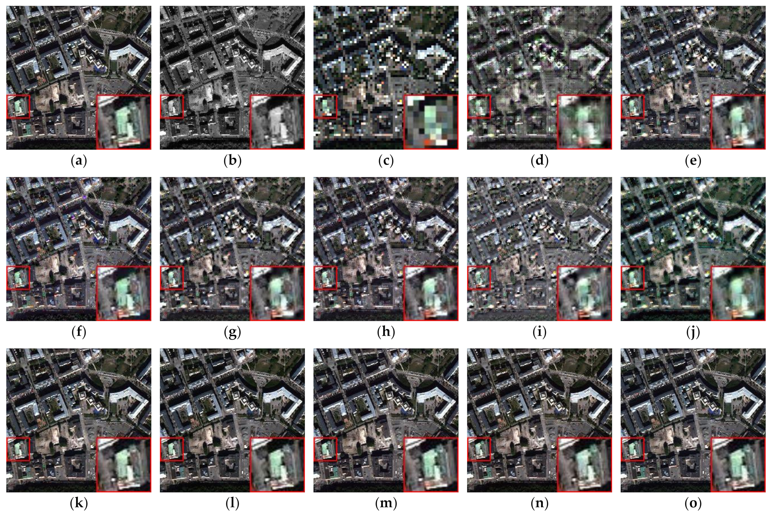
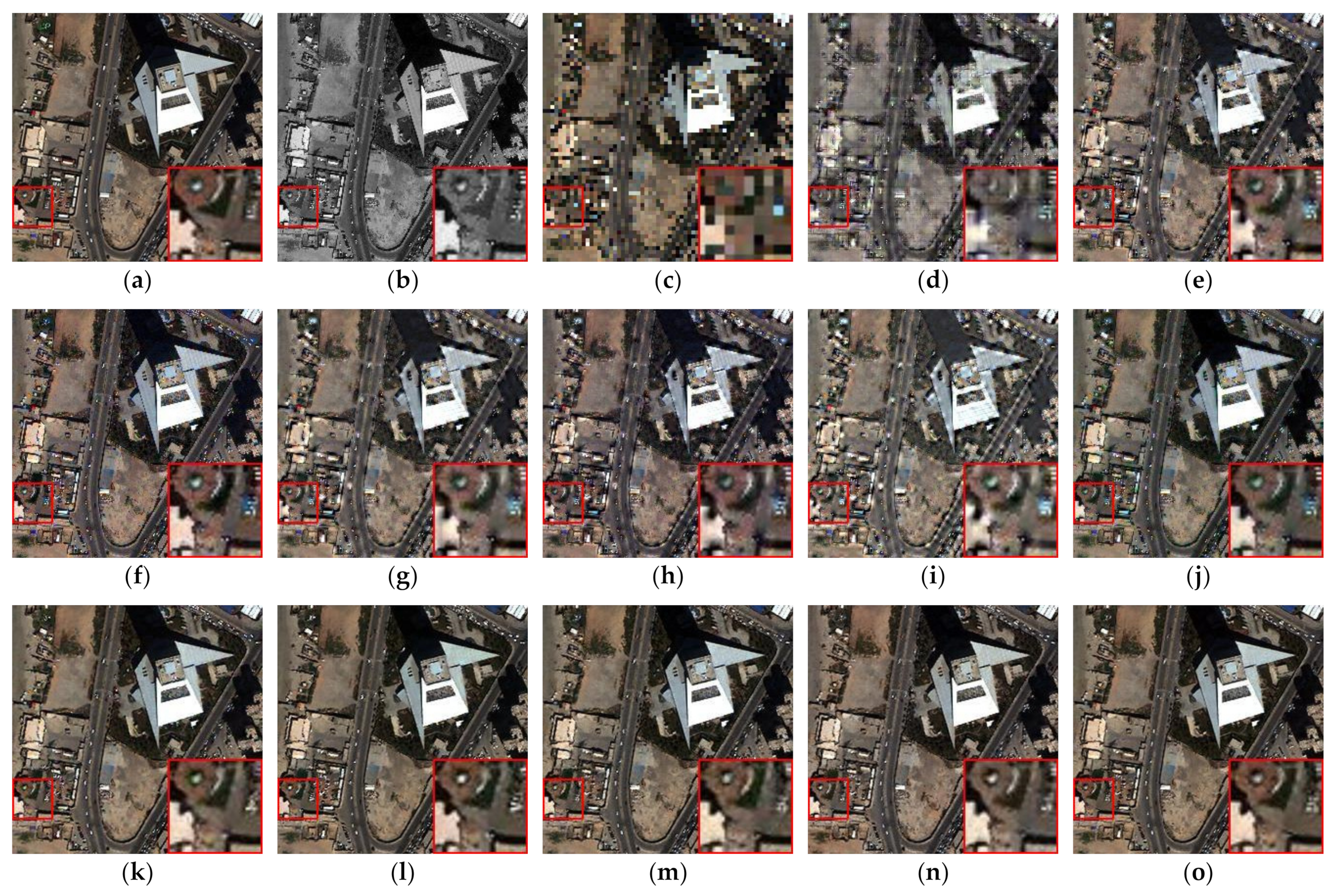
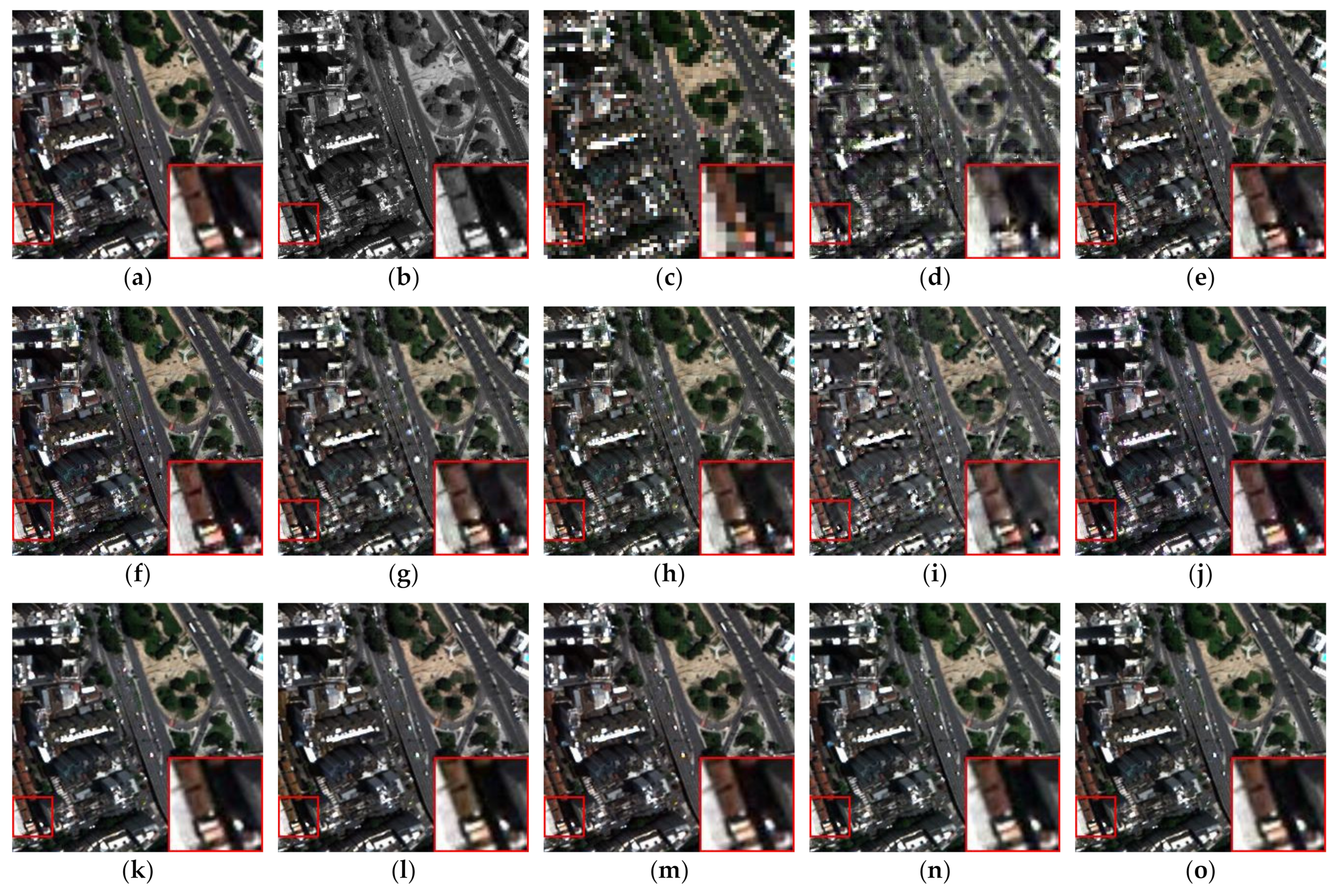
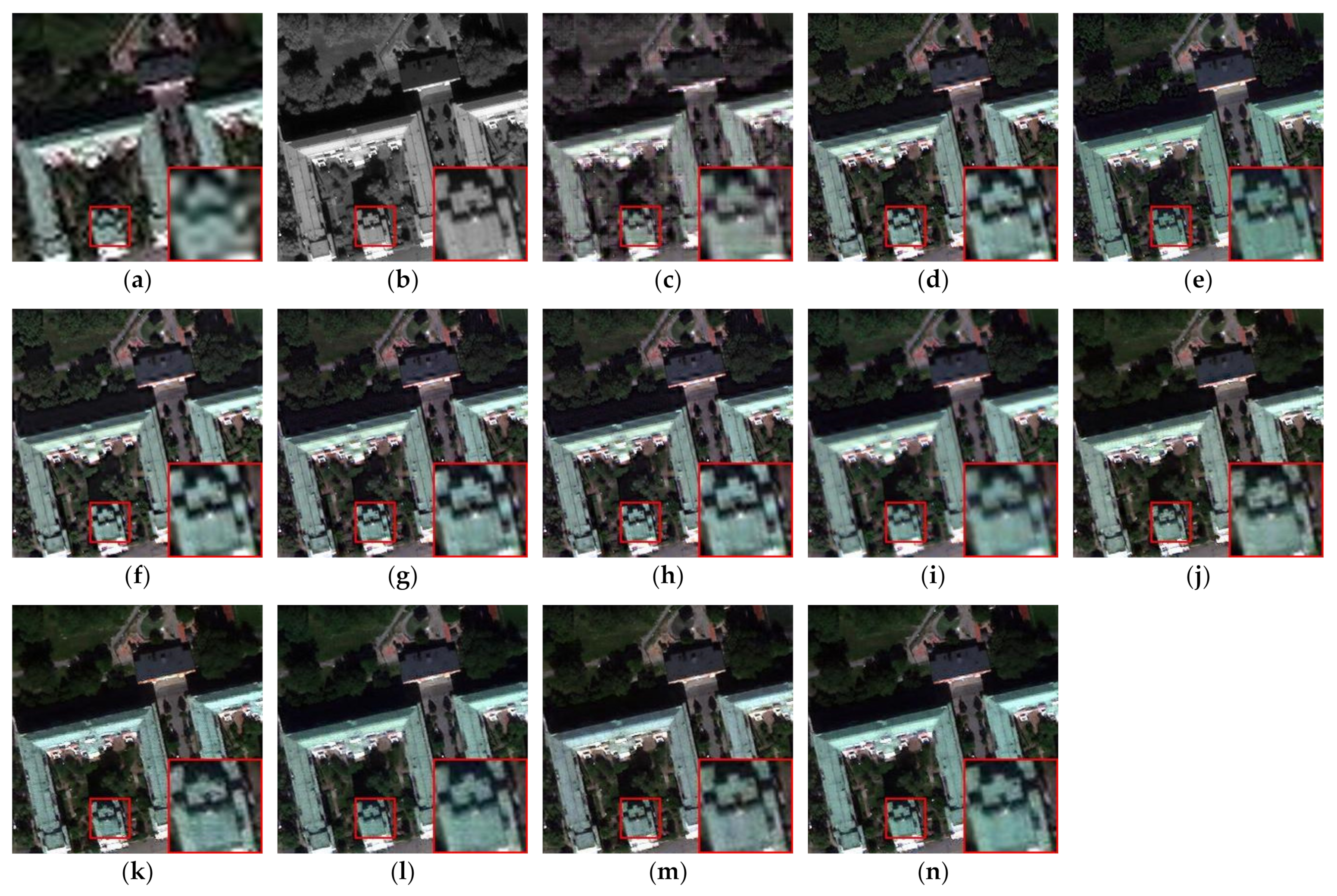
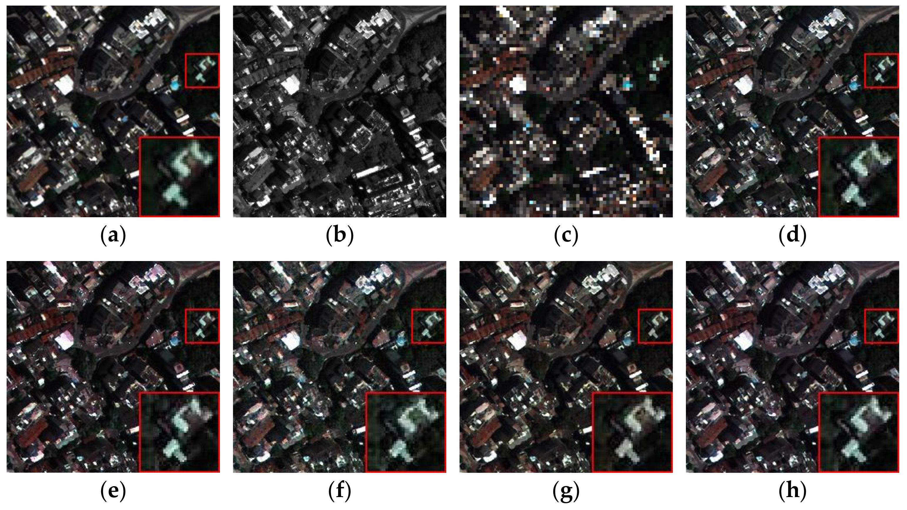
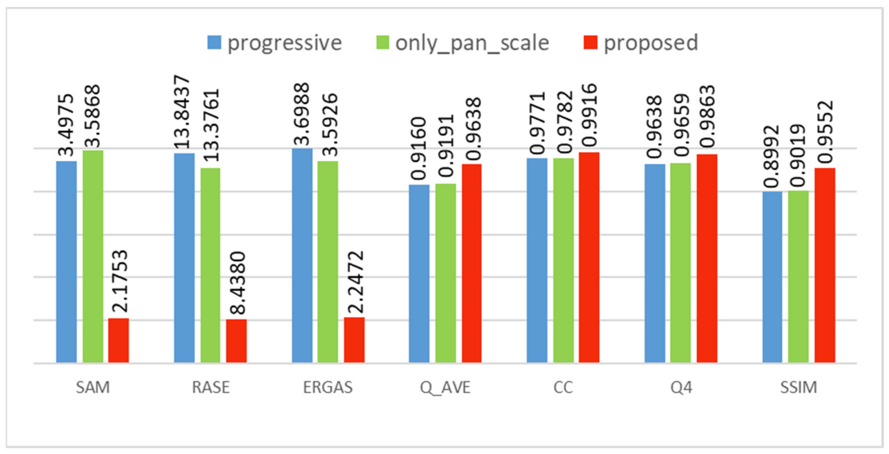
Table 1.
Spatial and radiometric resolution (RR) and number of bands for the satellite datasets.
| Sensors | Bands | PAN | MS | RR |
|---|---|---|---|---|
| QuickBird | 4 | 0.61 m | 2.44 m | 11 bit |
| WorldView-2 | 8 | 0.46 m | 1.84 m | 11 bit |
| WorldView-3 | 8 | 0.31 m | 1.24 m | 11 bit |
Table 2.
Size of the training and testing sets for the satellite datasets.
| Dataset | Total Numbers | Train Set | Validation Set |
|---|---|---|---|
| QuickBird | 950 | 750 | 200 |
| WorldView-2 | 750 | 600 | 150 |
| WorldView-3 | 1300 | 1000 | 300 |
Table 3.
Evaluation results on the QuickBird dataset. The mean and deviation values are shown in this table and in the following tables (best results in bold).
Table 3.
Evaluation results on the QuickBird dataset. The mean and deviation values are shown in this table and in the following tables (best results in bold).
| Method | SAM | RASE | Q_AVE | ERGAS | CC | Q4 | SSIM |
|---|---|---|---|---|---|---|---|
| DWT | 13.97 ± 1.17 | 43.90 ± 3.34 | 0.533 ± 0.047 | 10.96 ± 0.69 | 0.758 ± 0.028 | 0.701 ± 0.057 | 0.495 ± 0.041 |
| HPF | 10.35 ± 1.31 | 41.38 ± 2.34 | 0.638 ± 0.035 | 10.53 ± 0.41 | 0.831 ± 0.013 | 0.762 ± 0.034 | 0.613 ± 0.035 |
| GS | 8.88 ± 1.46 | 31.13 ± 3.06 | 0.686 ± 0.062 | 7.86 ± 0.43 | 0.888 ± 0.019 | 0.819 ± 0.048 | 0.662 ± 0.061 |
| GLP | 11.06 ± 1.47 | 41.83 ± 2.51 | 0.644 ± 0.037 | 10.65 ± 0.44 | 0.838 ± 0.013 | 0.768 ± 0.036 | 0.616 ± 0.037 |
| SFIM | 8.36 ± 0.99 | 43.45 ± 1.92 | 0.639 ± 0.022 | 11.33 ± 0.48 | 0.821 ± 0.009 | 0.745 ± 0.027 | 0.619 ± 0.021 |
| IND | 14.07 ± 1.79 | 51.59 ± 2.99 | 0.539 ± 0.038 | 13.13 ± 0.58 | 0.756 ± 0.013 | 0.665 ± 0.048 | 0.517 ± 0.036 |
| PRACS | 10.06 ± 1.25 | 37.99 ± 3.07 | 0.658 ± 0.04 | 9.39 ± 0.29 | 0.839 ± 0.032 | 0.794 ± 0.038 | 0.629 ± 0.038 |
| DMDNet | 4.25 ± 0.26 | 15.41 ± 0.79 | 0.877 ± 0.027 | 4.06 ± 0.17 | 0.976 ± 0.003 | 0.955 ± 0.014 | 0.863 ± 0.027 |
| CPNet | 4.03 ± 0.28 | 15.45 ± 1.36 | 0.888 ± 0.027 | 3.98 ± 0.19 | 0.975 ± 0.004 | 0.957 ± 0.014 | 0.877 ± 0.027 |
| TPNwFB | 2.63 ± 0.16 | 10.64 ± 0.79 | 0.939 ± 0.015 | 2.79 ± 0.15 | 0.988 ± 0.002 | 0.978 ± 0.007 | 0.934 ± 0.013 |
| TDPNet | 3.70 ± 0.25 | 14.14 ± 0.85 | 0.897 ± 0.023 | 3.65 ± 0.17 | 0.979 ± 0.003 | 0.962 ± 0.011 | 0.885 ± 0.022 |
| Proposed | 2.32 ± 0.13 | 9.29 ± 0.66 | 0.949 ± 0.013 | 2.41 ± 0.11 | 0.991 ± 0.001 | 0.983 ± 0.006 | 0.945 ± 0.012 |
| Ideal value | 0 | 0 | 1 | 0 | 1 | 1 | 1 |
Table 4.
Evaluation results on the WorldView-2 dataset (best results in bold).
| Method | SAM | RASE | Q_AVE | ERGAS | CC | Q4 | SSIM |
|---|---|---|---|---|---|---|---|
| DWT | 8.86 ± 0.64 | 31.86 ± 3.65 | 0.576 ± 0.016 | 7.98 ± 0.89 | 0.808 ± 0.029 | 0.734 ± 0.012 | 0.525 ± 0.013 |
| HPF | 7.76 ± 0.86 | 32.39 ± 4.26 | 0.649 ± 0.013 | 7.99 ± 1.07 | 0.838 ± 0.029 | 0.777 ± 0.012 | 0.616 ± 0.014 |
| GS | 6.17 ± 0.74 | 23.37 ± 3.92 | 0.723 ± 0.017 | 5.76 ± 0.98 | 0.899 ± 0.027 | 0.848 ± 0.017 | 0.686 ± 0.019 |
| GLP | 8.14 ± 0.94 | 32.19 ± 4.19 | 0.664 ± 0.015 | 7.94 ± 1.05 | 0.849 ± 0.028 | 0.788 ± 0.012 | 0.630 ± 0.015 |
| SFIM | 6.37 ± 0.78 | 33.62 ± 4.53 | 0.641 ± 0.014 | 8.29 ± 1.14 | 0.828 ± 0.033 | 0.764 ± 0.015 | 0.609 ± 0.014 |
| IND | 10.28 ± 1.48 | 40.05 ± 5.46 | 0.578 ± 0.011 | 9.88 ± 1.37 | 0.765 ± 0.041 | 0.698 ± 0.016 | 0.549 ± 0.013 |
| PRACS | 6.99 ± 0.82 | 26.29 ± 4.24 | 0.716 ± 0.013 | 6.45 ± 1.06 | 0.897 ± 0.027 | 0.839 ± 0.009 | 0.678 ± 0.016 |
| DMDNet | 5.05 ± 0.59 | 22.09 ± 3.29 | 0.783 ± 0.023 | 5.44 ± 0.82 | 0.923 ± 0.019 | 0.881 ± 0.015 | 0.751 ± 0.026 |
| CPNet | 4.59 ± 0.54 | 20.09 ± 2.82 | 0.807 ± 0.019 | 4.95 ± 0.69 | 0.931 ± 0.017 | 0.898 ± 0.011 | 0.777 ± 0.024 |
| TPNwFB | 4.24 ± 0.75 | 18.19 ± 2.98 | 0.826 ± 0.036 | 4.48 ± 0.74 | 0.944 ± 0.018 | 0.913 ± 0.017 | 0.796 ± 0.043 |
| TDPNet | 4.72 ± 0.68 | 18.66 ± 2.88 | 0.813 ± 0.031 | 4.59 ± 0.71 | 0.941 ± 0.018 | 0.907 ± 0.016 | 0.782 ± 0.036 |
| Proposed | 4.19 ± 0.71 | 17.74 ± 2.94 | 0.834 ± 0.029 | 4.36 ± 0.73 | 0.947 ± 0.017 | 0.918 ± 0.015 | 0.805 ± 0.036 |
| Ideal value | 0 | 0 | 1 | 0 | 1 | 1 | 1 |
Table 5.
Evaluation results on the WorldView-3 dataset (best results in bold).
| Method | SAM | RASE | Q_AVE | ERGAS | CC | Q4 | SSIM |
|---|---|---|---|---|---|---|---|
| DWT | 7.81 ± 0.59 | 30.43 ± 3.29 | 0.647 ± 0.033 | 7.75 ± 0.83 | 0.885 ± 0.006 | 0.791 ± 0.029 | 0.609 ± 0.029 |
| HPF | 4.29 ± 0.49 | 27.83 ± 3.92 | 0.735 ± 0.035 | 7.11 ± 1.04 | 0.912 ± 0.007 | 0.865 ± 0.021 | 0.715 ± 0.035 |
| GS | 3.79 ± 0.49 | 19.29 ± 2.88 | 0.804 ± 0.044 | 4.93 ± 0.77 | 0.951 ± 0.008 | 0.906 ± 0.022 | 0.786 ± 0.043 |
| GLP | 4.47 ± 0.52 | 27.44 ± 3.89 | 0.749 ± 0.037 | 7.02 ± 1.04 | 0.924 ± 0.007 | 0.873 ± 0.021 | 0.731 ± 0.036 |
| SFIM | 3.82 ± 0.44 | 43.85 ± 29.08 | 0.737 ± 0.034 | 12.83 ± 10.69 | 0.827 ± 0.154 | 0.848 ± 0.029 | 0.719 ± 0.032 |
| IND | 6.48 ± 0.99 | 36.23 ± 5.07 | 0.648 ± 0.039 | 9.23 ± 1.32 | 0.857 ± 0.009 | 0.795 ± 0.029 | 0.628 ± 0.038 |
| PRACS | 4.05 ± 0.42 | 20.54 ± 2.99 | 0.817 ± 0.034 | 5.13 ± 0.78 | 0.958 ± 0.007 | 0.917 ± 0.015 | 0.799 ± 0.031 |
| DMDNet | 2.93 ± 0.31 | 12.84 ± 1.92 | 0.899 ± 0.014 | 3.19 ± 0.48 | 0.978 ± 0.004 | 0.963 ± 0.006 | 0.895 ± 0.009 |
| CPNet | 3.05 ± 0.47 | 13.86 ± 2.31 | 0.897 ± 0.016 | 3.38 ± 0.54 | 0.974 ± 0.005 | 0.952 ± 0.012 | 0.895 ± 0.012 |
| TPNwFB | 2.87 ± 0.28 | 12.58 ± 1.96 | 0.894 ± 0.016 | 3.14 ± 0.49 | 0.979 ± 0.004 | 0.961 ± 0.007 | 0.888 ± 0.012 |
| TDPNet | 3.06 ± 0.34 | 12.61 ± 1.74 | 0.888 ± 0.021 | 3.15 ± 0.44 | 0.979 ± 0.004 | 0.956 ± 0.011 | 0.883 ± 0.016 |
| Proposed | 2.76 ± 0.28 | 12.16 ± 1.88 | 0.903 ± 0.019 | 3.03 ± 0.47 | 0.981 ± 0.004 | 0.963 ± 0.009 | 0.899 ± 0.015 |
| Ideal value | 0 | 0 | 1 | 0 | 1 | 1 | 1 |
Table 6.
Evaluation results of the QuickBird real dataset (best results in bold).
| Method | QNR | Dλ | DS |
|---|---|---|---|
| DWT | 0.583 ± 0.011 | 0.325 ± 0.024 | 0.136 ± 0.015 |
| HPF | 0.672 ± 0.006 | 0.129 ± 0.013 | 0.228 ± 0.019 |
| GS | 0.690 ± 0.032 | 0.076 ± 0.005 | 0.253 ± 0.030 |
| GLP | 0.670 ± 0.006 | 0.127 ± 0.014 | 0.233 ± 0.005 |
| SFIM | 0.686 ± 0.004 | 0.124 ± 0.016 | 0.217 ± 0.018 |
| IND | 0.728 ± 0.008 | 0.099 ± 0.010 | 0.192 ± 0.001 |
| PRACS | 0.805 ± 0.028 | 0.046 ± 0.002 | 0.156 ± 0.027 |
| DMDNet | 0.857 ± 0.022 | 0.063 ± 0.020 | 0.085 ± 0.010 |
| CPNet | 0.872 ± 0.022 | 0.053 ± 0.011 | 0.079 ± 0.014 |
| TPNwFB | 0.895 ± 0.012 | 0.048 ± 0.019 | 0.060 ± 0.008 |
| TDPNet | 0.902 ± 0.012 | 0.033 ± 0.005 | 0.067 ± 0.010 |
| Proposed | 0.914 ± 0.005 | 0.027 ± 0.008 | 0.061 ± 0.007 |
| Ideal value | 1 | 0 | 0 |
Table 7.
Evaluation results of deep learning methods trained on QuickBird and tested on WorldView-3 (best results is in bold).
Table 7.
Evaluation results of deep learning methods trained on QuickBird and tested on WorldView-3 (best results is in bold).
| Method | SAM | RASE | Q_AVE | ERGAS | CC | Q4 | SSIM |
|---|---|---|---|---|---|---|---|
| DMDNet | 4.99 ± 0.58 | 23.41 ± 3.91 | 0.799 ± 0.021 | 5.87 ± 1.00 | 0.938 ± 0.003 | 0.901 ± 0.012 | 0.778 ± 0.020 |
| CPNet | 5.79 ± 0.55 | 26.50 ± 3.81 | 0.749 ± 0.032 | 6.38 ± 0.95 | 0.918 ± 0.002 | 0.852 ± 0.028 | 0.728 ± 0.031 |
| TPNwFB | 5.93 ± 0.54 | 22.85 ± 3.07 | 0.716 ± 0.016 | 5.65 ± 0.77 | 0.931 ± 0.001 | 0.872 ± 0.022 | 0.670 ± 0.014 |
| TDPNet | 5.55 ± 0.45 | 22.19 ± 2.84 | 0.774 ± 0.021 | 5.41 ± 0.72 | 0.946 ± 0.001 | 0.879 ± 0.025 | 0.747 ± 0.017 |
| Proposed | 4.44 ± 0.45 | 19.47 ± 3.01 | 0.800 ± 0.022 | 4.83 ± 0.75 | 0.950 ± 0.002 | 0.907 ± 0.020 | 0.779 ± 0.020 |
| Ideal value | 0 | 0 | 1 | 0 | 1 | 1 | 1 |
Table 8.
Comparison of different deep learning methods in terms of perform time, model size, number of parameters, and floating-point operations per second.
Table 8.
Comparison of different deep learning methods in terms of perform time, model size, number of parameters, and floating-point operations per second.
| Method | Performance Time (S) | Model Size (MB) | Parameters (M) | FLOPs (G) |
|---|---|---|---|---|
| DMDNet | 0.3776 | 2.06 | 0.53 | 2.19 |
| CPNet | 0.1921 | 2.87 | 0.75 | 2.29 |
| TPNwFB | 1.6638 | 52.41 | 13.71 | 33.24 |
| TDPNet | 0.6529 | 47.31 | 12.36 | 5.03 |
| Proposed | 1.3364 | 38.53 | 9.97 | 7.34 |
Table 9.
Quantitative evaluation results of MLRB under different combinations, where “ms_” denotes multiscale, the numbers to the right of “ms” denote the large-kernel convolution size on each of the four branches, and “single_9+3” denotes only one feature composite without using dilated convolution, where the large-kernel convolutional size is 9 × 9 (best results in bold).
| Combination | SAM | RASE | Q_AVE | ERGAS | CC | Q4 | SSIM |
|---|---|---|---|---|---|---|---|
| Single_9 + 3 | 2.50 ± 0.13 | 9.91 ± 0.64 | 0.943 ± 0.014 | 2.56 ± 0.10 | 0.990 ± 0.001 | 0.981 ± 0.006 | 0.938 ± 0.012 |
| Dilate_3579 | 2.61 ± 0.16 | 10.08 ± 0.61 | 0.942 ± 0.014 | 2.61 ± 0.06 | 0.989 ± 0.002 | 0.980 ± 0.006 | 0.936 ± 0.012 |
| Ms_1579 | 2.41 ± 0.14 | 9.95 ± 0.67 | 0.945 ± 0.012 | 2.57 ± 0.10 | 0.989 ± 0.002 | 0.981 ± 0.006 | 0.939 ± 0.012 |
| Ms_3579 | 2.49 ± 0.16 | 9.97 ± 0.7 | 0.944 ± 0.013 | 2.57 ± 0.12 | 0.990 ± 0.001 | 0.981 ± 0.006 | 0.939 ± 0.013 |
| Ms_5579 | 2.56 ± 0.14 | 10.01 ± 0.64 | 0.942 ± 0.014 | 2.59 ± 0.09 | 0.989 ± 0.001 | 0.980 ± 0.006 | 0.937 ± 0.013 |
| Ms_7579 | 2.37 ± 0.14 | 9.39 ± 0.71 | 0.949 ± 0.013 | 2.44 ± 0.11 | 0.991 ± 0.001 | 0.983 ± 0.006 | 0.944 ± 0.012 |
| Proposed (ms_9579) | 2.32 ± 0.13 | 9.29 ± 0.66 | 0.949 ± 0.013 | 2.41 ± 0.11 | 0.991 ± 0.001 | 0.983 ± 0.006 | 0.945 ± 0.012 |
| Ms_13-579 | 2.45 ± 0.16 | 10.08 ± 0.77 | 0.944 ± 0.013 | 2.60 ± 0.13 | 0.990 ± 0.002 | 0.981 ± 0.006 | 0.939 ± 0.013 |
| Ms_31-579 | 3.70 ± 0.27 | 14.1 ± 1.07 | 0.900 ± 0.023 | 3.62 ± 0.21 | 0.979 ± 0.003 | 0.963 ± 0.010 | 0.890 ± 0.023 |
| Ideal value | 0 | 0 | 1 | 0 | 1 | 1 | 1 |
Table 10.
Results of the quantitative evaluation of double-stack aggregated skip connections and CRAB (best results in bold).
Table 10.
Results of the quantitative evaluation of double-stack aggregated skip connections and CRAB (best results in bold).
| Method | SAM | RASE | Q_AVE | ERGAS | CC | Q4 | SSIM |
|---|---|---|---|---|---|---|---|
| No_first_layer | 2.61 ± 0.18 | 11.10 ± 0.76 | 0.937 ± 0.014 | 2.85 ± 0.13 | 0.987 ± 0.002 | 0.977 ± 0.007 | 0.931 ± 0.013 |
| Origin_Resnet | 2.69 ± 0.16 | 10.53 ± 0.91 | 0.940 ± 0.017 | 2.72 ± 0.20 | 0.988 ± 0.002 | 0.977 ± 0.007 | 0.932 ± 0.015 |
| Using_RFA | 2.52 ± 0.17 | 10.22 ± 0.87 | 0.943 ± 0.014 | 2.64 ± 0.12 | 0.989 ± 0.002 | 0.980 ± 0.007 | 0.937 ± 0.014 |
| Proposed | 2.32 ± 0.13 | 9.29 ± 0.66 | 0.949 ± 0.013 | 2.41 ± 0.11 | 0.991 ± 0.001 | 0.983 ± 0.006 | 0.945 ± 0.012 |
| Ideal value | 0 | 0 | 1 | 0 | 1 | 1 | 1 |
Publisher’s Note: MDPI stays neutral with regard to jurisdictional claims in published maps and institutional affiliations. |
© 2022 by the authors. Licensee MDPI, Basel, Switzerland. This article is an open access article distributed under the terms and conditions of the Creative Commons Attribution (CC BY) license (https://creativecommons.org/licenses/by/4.0/).
Share and Cite
MDPI and ACS Style
Li, W.; He, M.; Xiang, M. Double-Stack Aggregation Network Using a Feature-Travel Strategy for Pansharpening. Remote Sens. 2022, 14, 4224. https://0-doi-org.brum.beds.ac.uk/10.3390/rs14174224
AMA Style
Li W, He M, Xiang M. Double-Stack Aggregation Network Using a Feature-Travel Strategy for Pansharpening. Remote Sensing. 2022; 14(17):4224. https://0-doi-org.brum.beds.ac.uk/10.3390/rs14174224
Chicago/Turabian StyleLi, Weisheng, Maolin He, and Minghao Xiang. 2022. "Double-Stack Aggregation Network Using a Feature-Travel Strategy for Pansharpening" Remote Sensing 14, no. 17: 4224. https://0-doi-org.brum.beds.ac.uk/10.3390/rs14174224
Note that from the first issue of 2016, this journal uses article numbers instead of page numbers. See further details here.