HY-1C/D Reveals the Chlorophyll-a Concentration Distribution Details in the Intensive Islands’ Waters and Its Consistency with the Distribution of Fish Spawning Ground

Abstract

Chlorophyll-a (Chl-a) change details derived from HY-1C/D images in the waters of the Zhoushan archipelago were analyzed. A new Chl-a inverse model was built based on the relationship between the in situ Chl-a and the combination of red, blue and green bands of the coastal zone imager (CZI). Chl-a as well as fishery resources were analyzed. The results showed the following. (1) The Chl-a concentration in the waters of the Zhoushan archipelago was mainly in the range of 0.5~6 μg/L. High Chl-a area distributed in the west side of the study area, with a value of 3.5~5.5 μg/L. The Chl-a concentration in the east side of the study area was relatively lower, with a value of 0.5~2 μg/L. Chl-a around the islands was higher than that in the area far away from the islands. In addition, Chl-a concentration increased obviously downstream of the island. (2) The spawning ground of many fish in the waters of the Zhoushan archipelago was abundant, and its spatial-temporal variation was consistent with the change of Chl-a. (3) The islands interacted with the current, inducing upwelling upstream and vortex streets downstream. The complex hydrodynamic environment promoted a vertical exchange of water bodies, thereby resulting in an increase in suspended sediment concentration, nutrients, Chl-a and attracting fish.

1. Introduction

Chl-a is an important factor for evaluating water quality and assessing the levels of organic pollution and predicting the fishery [1]. It is one of the main elements of ocean color. In the past, analyzing the distribution of Chl-a was mainly based on field measured data, from the early measurement of the water sample in a laboratory on the ship to the later ship testing [2], which was expensive and ineffective.

With the characteristics of large scale and quasi-synchronous [3], remote sensing can perform a relatively precise observation of Chl-a distribution in the ocean. Many studies have been conducted based on remote sensing. The early Chl-a concentration retrieval research in the water was mainly focused on case I water, whose optical character is mainly determined by the concentration of Chl-a; the other ocean color elements are relatively low and have little impact on the inversion accuracy. The algorithms of the retrieval of Chl-a in case I water, such as the blue–green ratio method [4], the inherent optical properties (IOP) method [5] and the fluorescence algorithm [6], are relatively mature. However, in case II waters, especially those in the mouth of estuaries, coastal zones influenced by river runoff, etc. [7,8], there are high concentrations of total suspended matter (TSM) and colored dissolved organic matter (CDOM). The backscattering of TSM [9] and the strong absorption of CDOM [10] directly affect the optical property of seawater; the algorithms fit for case I water are no longer fully applicable for case II water and need to be improved and modified.

More and more researchers began to develop the retrieval model for Chl-a concentration in case II water. The Chl-a concentration was successfully calculated based on the ratio of the red and infrared band in 1990 [11]. Later, in 1994, Tassan [12] proposed a set of statistical inversion algorithms for the Mediterranean waters based on the band ratio to retrieve three elements of ocean color using the bands determined by the spectral characteristics of different ocean color elements. Furthermore, the statistical model of Chl-a concentration in the coastal waters of the East China Sea was developed based on high-quality in situ data [13]. Combining the 412 nm, 443 nm, 490 nm and 555 nm remote-sensing reflectance of the geostationary ocean color imager (GOCI), a band ratio model was established and applied to analyze the Chl-a concentration in the Bohai Sea and Yellow Sea [14]. In recent years, a variety of studies were performed using different kinds of satellite data, such as the coastal zone color scanner (CZCS) [15], ocean color and temperature scanner (OCTS) [16], ocean color monitor (OCM) [17], sea-viewing wide field sensor (SeaWiFS) [8], moderate-resolution imaging spectroradiometer (MODIS) [18], medium-resolution imaging spectrometer (MERIS) [19], Landsat thematic mapper (TM) [20], etc. With the rapid development of satellites in China, more and more researchers have applied HY-1A/B [21], China–Brazil Earth Resource Satellite (CBERS) [22], GF-1 [23], HJ-1A/B [24], to conduct ocean color research. HY-1C/D CZI can obtain real-time image data of the land–sea interaction area for coastal monitoring, and it has great potential in monitoring the water quality in estuaries and harbors. However, the former built models for retrieving Chl-a concentration in coastal waters, such as OC3 [25], OC4 [26], etc., are not suitable for the band setting of CZI. Therefore, it is urgent to build an inverse model suitable for the coastal waters based on HY-1C/D CZI data.

Zhoushan intensive islands area is in the center of the Zhoushan Fishery, and it is rich in fishery resources. Historically, it was one of the highest yield fisheries, as well as an important spawning ground and feeding ground for many economical fish species in China [27]. The water in the Zhoushan area is typical case II water, with the domination of TSM [28], making its composition very complex.

This paper mainly focused on the waters of the Zhoushan archipelago and analyzed the Chl-a distribution details and its relationship with fish spawning grounds. This study can improve the existing water quality monitoring method and provide a scientific basis for the rational use and protection of fishery resources in the waters of the Zhoushan archipelago.

2. Data and Methods

2.1. Study Area

Located in the east of the Hangzhou Bay and southeast of the Yangtze River estuary, Zhoushan Islands are the easternmost archipelago in the western Pacific Ocean in China. It is composed of intensive islands and has a subtropical monsoon climate [29].

Zhoushan intensive islands area is in the center of the Zhoushan Fishery. The water there is mainly affected by the East China Sea, the Changjiang diluted water, as well as the runoff of the Qiantang River (Figure 1). In addition, the northern cold water mass of the Yellow Sea and the southern Kuroshio Current [30] also contribute to the complex hydrological environment of this area. The complex geographical environment gives this area the characteristics of broad temperature, low salinity and low transparency [31]. It is rich in aquatic product resources, with more than 500 kinds of marine life, including hairtail, large and small yellow croaker and cuttlefish [32]. Meanwhile, the Zhoushan intensive islands area is also an important combination port and the main traffic route of Ningbo-Zhoushan.

Zhoushan Fishery is the main fishery [32] for the four major economic fish: large yellow croaker, small yellow croaker, cuttlefish and hairtail. In the southern part of the study area, Daiquyang is a place where the famous large yellow croaker of the Daiquyang tribe used to spawn, breed and feed [33]. Additionally, it is also the main spawning ground for the large yellow croaker, half-in anchovy, Japanese Spanish mackerel, cuttlefish, white croaker, silver pomfret, Bloch and anchovy [30].

2.2. Satellite Data

HY-1C/D, launched on 7 September 2018 and 11 June 2020, respectively, both load a visible payload CZI. The launch of HY-1C has successfully ushered in a new era of integrated land–sea development of Chinese natural resources satellites. Together with the HY-1D launched later, these two satellites form a double star observation network in the morning and in the afternoon. With its characteristics of high resolution (50 m), covering commonly used bands (including visible light band and near-infrared band), big ground sweep width (950 km), relatively short playback period (3 days) and free access, CZI has a competitive advantage in the retrieval of Chl-a. The detailed wavelength settings for HY-1C/D CZI are shown in

Table 1. Band information of HY-1C/D CZI.

Sensor	Band No.	Spectral Range/μm
HY-1C CZI	Band 1 (Blue)	0.421–0.500
	Band 2 (Green)	0.517–0.598
	Band 3 (Red)	0.608–0.690
	Band 4 (NIR)	0.761–0.891

.

HY-1C/D are both equipped with five payloads, including coastal zone imager (CZI), Chinese ocean color and temperature scanner (COCTS), ultraviolet imagery (UV), satellite calibration spectrometer (SCS) and automatic identification system (AIS). All the payloads are provided with different levels of products. The different levels of CZI data are shown as follows. L1A data were obtained after the process of geometric calibration, and we obtained L1B data after a radiometric calibration of L1A. After atmospheric correction, L1B data become L2A data, which is the basis of all the ocean parameter products. L2B is the ocean color parameter product, including suspended sediment concentration (SSC) and the normalized difference vegetation index (NDVI), and L2C is the ocean color product, including Secchi disk depth (SDD) and Chl-a. We applied level L2A in this paper, which is the original data processed after geometric calibration, radiometric calibration and atmospheric correction. The L2A data are only processed for Rayleigh scattering. For coastal waters, the aerosol scattering is obvious and should not be ignored. Therefore, we performed aerosol scattering correction on L2A in our study. Moreover, to minimize the impact of aerosol, we also selected the satellite data on sunny and dry days.

The SST data were derived from the L3 product of MODIS, which was retrieved from the thermal infrared band data (band 31–32, daytime), with the spatial resolution of 4 km. These data can show the SST change in the waters of the Zhoushan islands area.

2.3. In Situ Data and Process

The in situ data consist of two seasonal cruises and one extra day cruise. The summer one is from 10 August to 17 August 2020, and the winter one is from 29 November to 10 December 2020. The extra day is 3 October 2019. The distribution of the sampling points is shown in Figure 2.

In situ Chl-a concentration is obtained based on the following steps. The first step is the sampling and filtering. Inject 0.5–2 L of the collected sea surface water sample into the sample bottle; use the GF/C filter membrane, suction filtration less than 50 kPa; after suction filtration is completed, use the ordinary filter; press on it to remove the water on the filter membrane as much as possible. Afterward, store the filter membrane in a refrigerator at −20 ℃ until the end of the voyage and return to the laboratory for measurement. The second step is extraction. Using a glass mortar, cut the filter membrane into small pieces and add 7–8 mL of 90% ethanol solution, and grind it into homogenate. Move the homogenate to a graduated centrifuge tube; rinse the mortar with a little extraction solution; merge the rinse solution into the centrifuge tube while shaking it; after that, place it in a dark and low-temperature environment for 12 h extraction. The third step is centrifugation. Put the centrifuged tube into the centrifuge, centrifuge for 10–15 min at a speed of 3500–4000 rpm. After that, take the upper layer. For the remaining extract, use it for double centrifugation. Set the volume of the solution obtained by the first and second centrifugation to 10 mL. The final step is determination. Using a 90% ethanol solution as a reference solution, the final Chl-a concentration is calculated by spectrophotometry, setting up two parallel samples for all the samples and taking the average of the two measurements as the final data [34].

In total, 130 in situ measurements were derived, of which 60 were used to establish the inversion model, and the remaining 70 were used to verify the retrieval results.

2.4. Wind

To obtain the wind characteristics in the study area, the product of an unstructured grid, the finite volume coastal ocean model (FVCOM) was applied. FVCOM is an ocean circulation and ecological model developed by Dr. Beardsley of the Woods Hole Oceanographic Institution in collaboration with the Ocean Eco dynamics Modeling Laboratory led by Dr. Chan Changsheng at the University of Massachusetts [35]. The FVCOM model horizontally adopts a triangular mesh model and vertically adopts a coordinate transformation, and the numerical method adopts the finite volume, which can simulate the original governing equation of the measurements of the free surface [36] and can more realistically fit the complex and tortuous coastline changes in the region. The governing equation of the mode is as follows.

$$\frac{\partial \zeta }{\partial t}+\frac{\partial Du}{\partial x}+\frac{\partial Dv}{\partial y}+\frac{\partial \omega }{\partial t}=0$$

(1)

$$\frac{\partial uD}{\partial t}+\frac{\partial u^{2}D}{\partial x}+\frac{\partial uvD}{\partial y}+\frac{\partial u\omega }{\partial \sigma }-fvD=-gD\frac{\partial \zeta }{\partial x}-\frac{gD}{{\rho }_0}\left[\frac{\partial }{\partial x}\left(D\underset{\sigma }{\overset{0}{{\displaystyle \int }}}\rho d{\sigma }^{\prime }\right)+\sigma \rho \frac{\partial D}{\partial x}\right]+\frac{1}{D}\frac{\partial }{\partial \sigma }\left(K_m\frac{\partial u}{\partial \sigma }\right)+D{F}_x$$

(2)

$$\frac{\partial vD}{\partial t}+\frac{\partial v^{2}D}{\partial y}+\frac{\partial uvD}{\partial x}+\frac{\partial u\omega }{\partial \sigma }+fuD=-gD\frac{\partial \zeta }{\partial y}-\frac{gD}{{\rho }_0}\left[\frac{\partial }{\partial y}\left(D\underset{\sigma }{\overset{0}{{\displaystyle \int }}}\rho d\sigma ’\right)+\sigma \rho \frac{\partial D}{\partial y}\right]+\frac{1}{D}\frac{\partial }{\partial \sigma }\left(K_m\frac{\partial v}{\partial \sigma }\right)+D{F}_y$$

(3)

where x, y, z are the east north and vertical axes in a $\sigma –$coordinate system; u, v, w are the x, y, z velocity components; t is the time variable. K_m is the vertical eddy viscosity coefficient; $\rho$ is the density; F_x, F_y represent the horizontal momentum; f is the Coriolis parameter; g is the gravitational acceleration; D is the total water column depth; and $\zeta$ is the height of the free surface (relative to z = 0).

2.5. Data Processing

The waters of the Zhoushan archipelago are dominated by TSM. The Rayleigh correction can eliminate most of the atmospheric influence, after which, we can effectively retrieve the Chl-a data. Based on the theory mentioned above, we chose images on dry sunny days, which can effectively reduce the impact of aerosol. HY-1C/D CZI Rayleigh corrected reflectance products (L2A) were obtained from the national satellite Ocean Application Center (https://osdds.nsoas.org.cn/, accessed on 21 December 2021) from January 2019 to November 2021. The products include the blue, green, red, near-infrared bands, which can be used to establish a Chl-a concentration inversion model suitable for the waters of the Zhoushan archipelago.

The remote-sensing reflectance (Rrs) can be obtained after precise atmospheric correction, including the Rayleigh correction and the correction of aerosol scattering. Since the Rayleigh correction is already processed, the aerosol correction for CZI is based on the MODIS aerosol data [37]. The normalized difference water index (NDWI) was applied to retrieve the land mask. Finally, we applied the atmospheric correction algorithm to propose HY-1C/D CZI data in turbid waters to obtain the Rrs [38].

All calculations were performed in the Python 3.8 and Envi 5.3 software.

3. Results

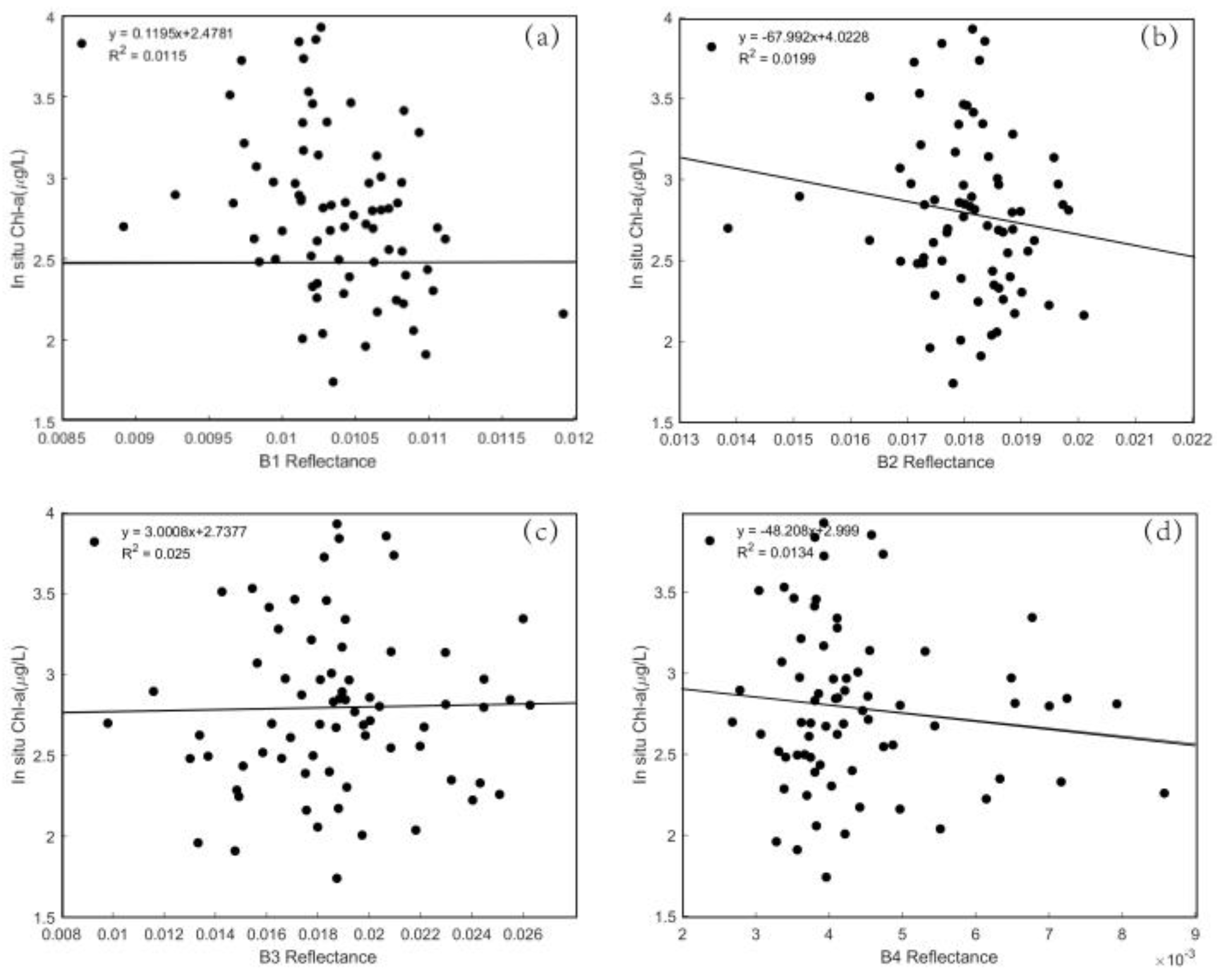
3.1. Sensitive Bands of Chl-a

To choose the sensitive band of Chl-a, the correlation coefficient between the Rrs of B1~B4 bands and in situ Chl-a concentration was analyzed (Figure 3).

The correlation coefficients of bands 1 to 4 are 0.0115, 0.0199, 0.025 and 0.0134, respectively, indicating that a single band is not sensitive to the change of Chl-a concentration. Therefore, it is necessary to analyze the sensitivity of band combination to assess Chl-a concentration.

3.2. Band Combination

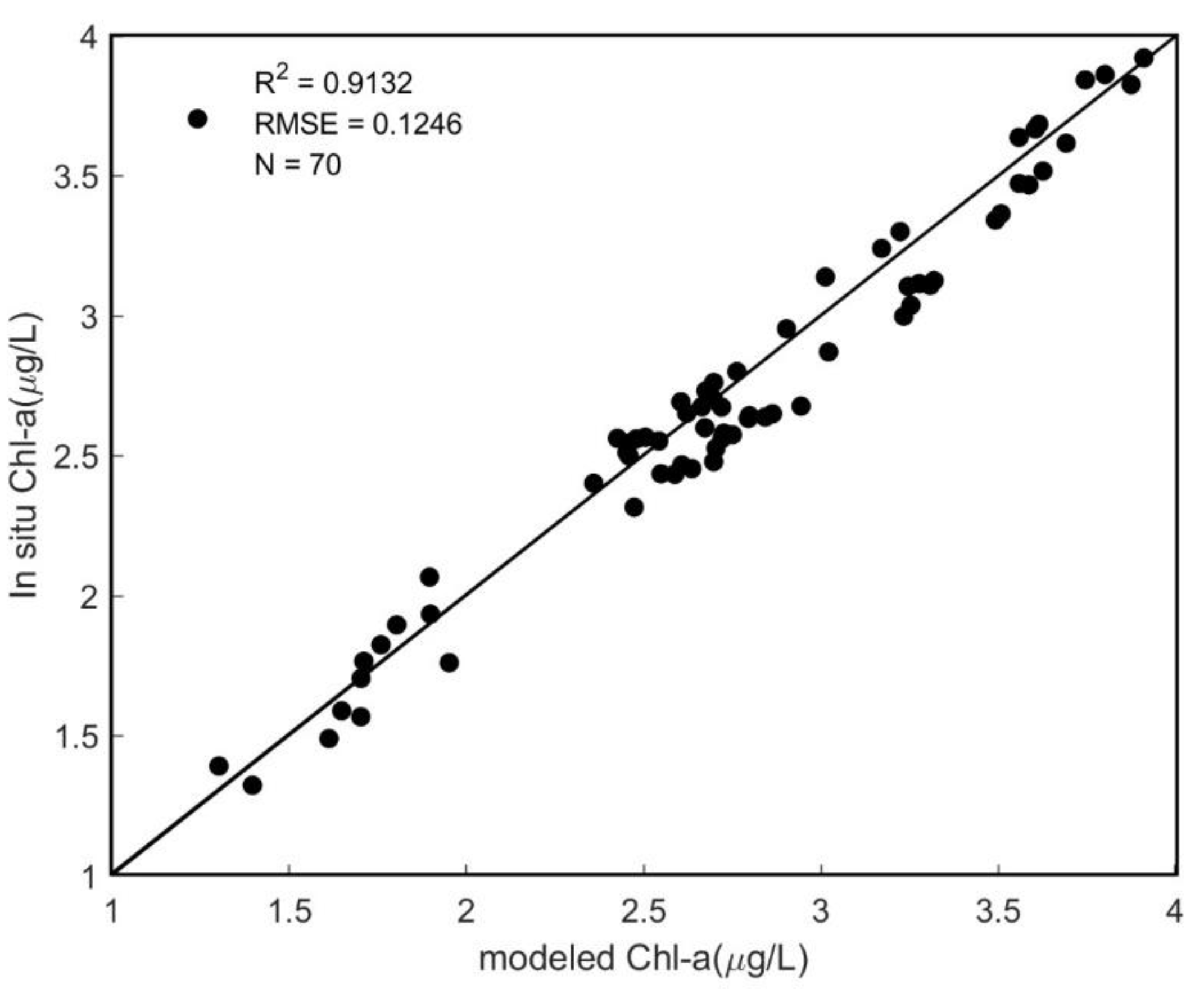
As the correlation between the single band and the in situ data is too low to build a model, the band combination is commonly used in the empirical model [39]. Previous research has shown that the ratio method can also greatly reduce the ocean bidirectional reflection problem [16]. To build a model, we need to find out which band combination is the most sensitive to the change of Chl-a concentration; therefore, a comparison was conducted to find the optimal band combination. High-correlation (>0.6) band combinations related to our study are shown in

Table 2. Band combination and R².

Band Combination(X)	$\mathbf{Correlation} \mathbf{Coefficient} \left({\mathbf{R}}^2\right)$
(B3 − B1)/((B3 + B1) × (B3/B2)0.45)	0.94
B3/((B1 + B2) × (B3/B2)0.45)	0.88
Log(B3/B2)	0.83
Log((B3/B1) × (B3/B2)0.45)	0.95
(B3 − B2)/(B3 + B2)	0.817
B4/(B2 + B4)	0.71
B4/(B1 + B3)	0.53
(B4 − B3)/(B4 + B3)	0.95
B3/(B1 + B3)	0.95
B3/(B2 + B3)	0.81
(B2 − B4)/(B2 + B3) × (B3/B2)0.45	0.62
Log(B3/B4)	0.69
(B1 − B4)/(B1 + B4)	0.80
B1 × B2/B3	0.67
(B1 × B3)/(B2 × B4)	0.49
(B1/B2) × (B3/B2)−0.45	0.96

B1, B2, B3, B4 represent the four bands of CZI, and the bold italics represent the optimal combination.

.

The data group was applied to establish models by linear, polynomial and exponential models. The band combination with the suspended sediment correction factor was more correlated than the other band combinations. Based on the blue–green ratio and the red–green ratio, which is a suspended sediment correction factor, the band combination X ((B1/B2) × (B3/B2)^−0.45) proved to be sensitive to Chl-a with R² of 0.96. As this combination was the one with the highest correlation, we therefore chose this band combination to build our retrieval model.

3.3. Model Building

Based on the above analysis, the linear, quadratic and exponential fittings were performed for the selected eight band combinations and measured Chl-a data, respectively, and 17 models were fitted, as shown in

Table 3. Models of band combinations and the corresponding correlation coefficients (R²) and RMSE.

Band Combination(X)	Function	Fitting Model	${\mathbf{R}}^2$	$\mathbf{RMSE} (\mathit{\mu }\mathit{g}/\mathit{L})$
B3/(B2 + B3)	Exponential	$\mathrm{Exp}(0.9515 \times {\mathrm{X}}^2$ + 4.506 × X − 1.684	0.83	0.0368
B3/(B2 + B3)	Sum of sine	29.93 × sin(0.5394 × X + 18.4)	0.82	0.1106
B3/(B2 + B3)	Gaussian	12.15 × $\mathrm{Exp}(-((\mathrm{X}-1.138)/0.4604{)}^2$)	0.82	0.1095
B3/(B2 + B3)	Exponential	0.1402 × Exp(5.542 × X)	0.80	0.0039
(B1 − B3)/(B1 + B4)	Polynomial	$0.2997 \times {\mathrm{X}}^2$ − 0.5954 × X + 1.054	0.55	0.0464
B4/(B1 + B2)	Polynomial	$45.85 \times {\mathrm{X}}^3$$-46.98 \times {\mathrm{X}}^2$ + 17.88 × X + 0.3271	0.49	0.1379
B3/(B1 + B3)	Exponential	0.05077 × Exp(5.916 × X)	0.89	0.0638
B3/(B1 + B3)	Exponential	$\mathrm{Exp}(13.14 \times {\mathrm{X}}^{3.975}$)	0.88	0.0638
Log(B3/B1)	Exponential	0.7367 × Exp(0.6388 × X)	0.90	0.0605
Log(B3/B1)	Power	1.062 × X1.303	0.88	0.0629
(B3 − B1)/(B3 + B1)	Exponential	Exp(0.2919 × Exp(3.516 × X)	0.92	0.0221
(B3 − B1)/(B3 + B1)	Exponential	Exp(2.88 × X + 0.004282)	0.87	0.0238
(B3 − B1)/(B3 + B1)	Rational	Exp(9985 × X − 518.4)/(X + 2970)	0.91	0.0204
(B3 − B1)/(B3 + B1)	Sum of sine	Exp(13.28 × sin(0.252 × X + 6.27))	0.9	0.02309
(B3 − B1)/(B3 + B1)	Polynomial	74.37 × X2 − 43.35 × X + 8.789	0.91	0.0545
(B1/B2) × ((B3/B2)−0.45	Polynomial	−12.81 × X3 + 38.17 × X2 − 39.17 × X + 14.9	0.95	0.0325
(B3 − B1)/((B3 + B1) × (B3/B2)0.45)	Exponential	Exp(1.208 × X2 − 2.4583 × X + 5.7829)	0.87	0.045

X: band combination; R²: the correlation coefficient; RMSE: the root mean square error, The bold italics represent the optimal model.

. The combination method with the largest correlation coefficient was selected to establish a Chl-a inverse model.

According to the evaluation results, a cubic polynomial fitting model based on the band ratio of band 1 (Blue), band 2 (Green) and band 3 (Red) was the best model, with the R² of 0.95 and RMSE of 0.0325 $\mathsf{\mu }$g/L (Table 2).

Therefore, the model for Chl-a inversion in the waters of the Zhoushan archipelago of CZI data (named SS-1) was finally determined (Equation (4)).

$$\rho =\mathrm{-12.81} \times {\mathrm{X}}^3 + 38.17 \times {\mathrm{X}}^2 – 39.17 \times \mathrm{X} + 14.9$$

(4)

$$\mathrm{X}=\left(\right(\mathrm{B}1/\mathrm{B}2) \times {(\mathrm{B}3/\mathrm{B}2)}^{\mathrm{-0.45}})$$

(5)

where $\rho$ is the Chl-a concentration; the unit is ug/L; B1, B2 and B3 are the reflectance of the first, second and third band of the CZI data, respectively.

The Chl-a inverse model Equation (5) was established based on X. It is an empirical algorithm for the Chl-a based on spectral characteristics and suitable for case 2 waters. The model was developed based on the satellite data and in situ data collected from the waters of the Zhoushan archipelago. It is a regional model and can be used in the water of the Zhoushan archipelago, where the suspended sediment concentration is in the range of 300–1200 mg/L, and the Chl-a concentration is in the range of 0.5–6 μg/L. To verify the feasibility of the newly built model, the modeled Chl-a was verified using in situ Chl-a data.

To assess the model’s accuracy, we used the root mean square error (RMSE) (Equation (6).)

$$\mathrm{RMSE}=\sqrt{\frac{1}{N}{\displaystyle \sum }_{i=1}^n{(Chl-a_i^{estimated}-Chl-a_i^{measured})}^2}$$

(6)

where ${Chl-a}_i^{estimated}$ is the model estimate value; ${Chl-a}_i^{measured}$ is the field measurement value; and n is the number of sample points.

The correlation coefficients of modeled Chl-a and in situ Chl-a were analyzed and showed a significant result with ${\mathrm{R}}^2$ = 0.91, RMSE = 0.12 (Figure 4), indicating that the newly built model based on CZI is suitable for inversion of Chl-a in the waters of the Zhoushan archipelago.

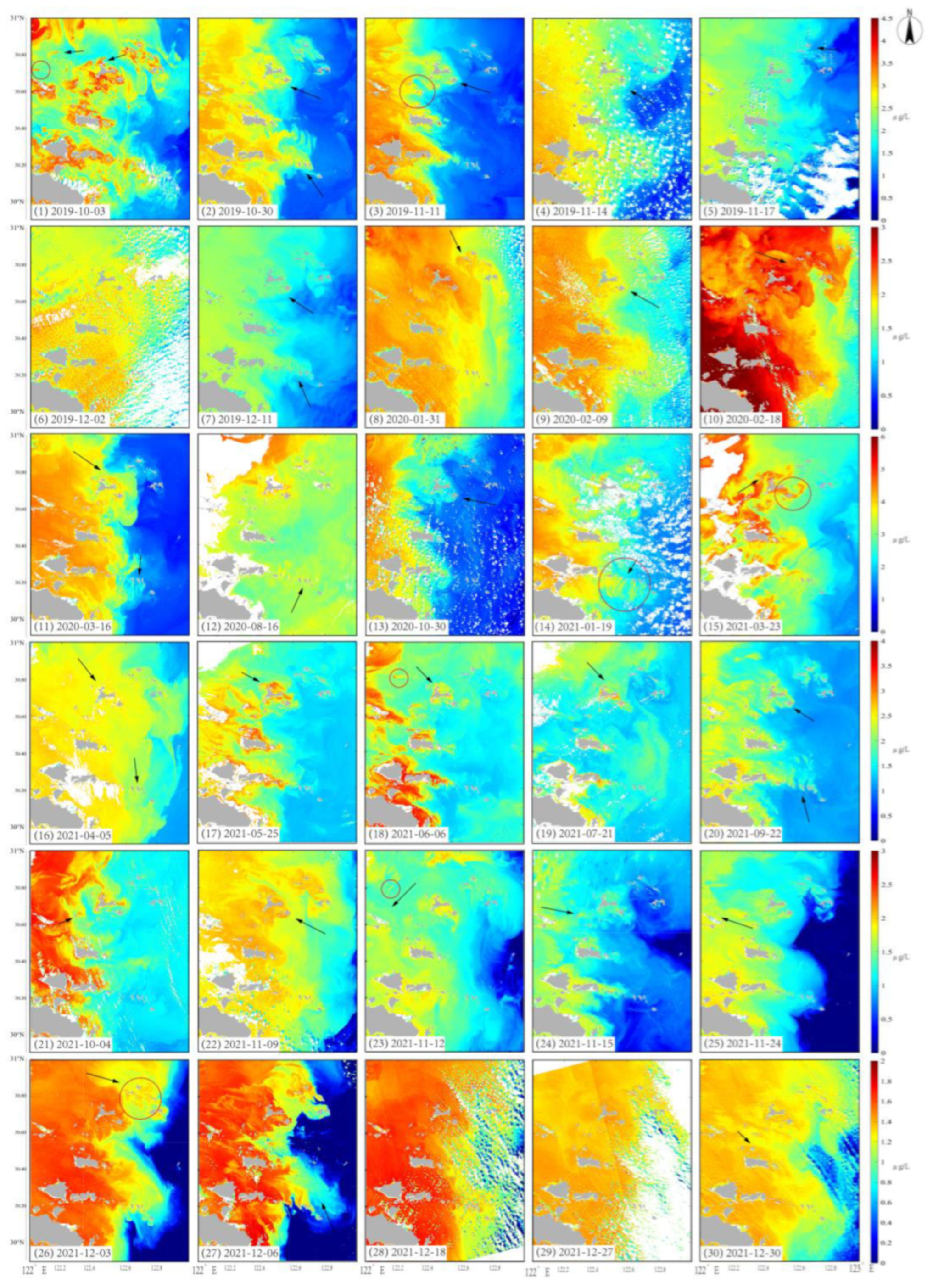
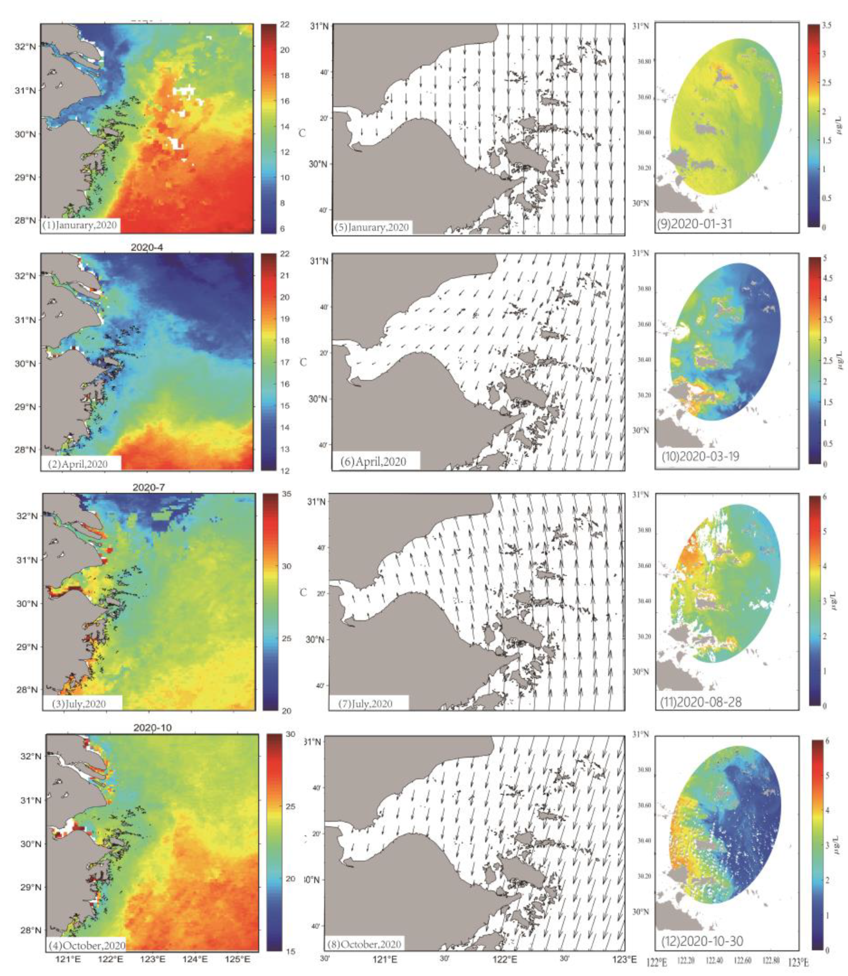
3.4. Chl-a in Shengsi-Centered Area

Chl-a distribution in the study area from September 2019 to November 2021 was retrieved based on the newly built model. A total of 48 CZI images of HY-1C from October 2019 to March 2021 and HY-1D from April 2021 to November 2021 were analyzed, and 30 of them are shown in Figure 5 as examples.

Chl-a concentration retrieved by the newly built model from the waters of the Zhoushan archipelago was mainly in the range of 0.5–6 μg/L. High Chl-a area distributed in the west side of the study area, about 2 μg/L higher, on average, than the area with lower Chl-a concentration on the east side. Chl-a distribution changes with the change of the currents. When the currents pass through the island, Chl-a concentration downstream of the island becomes higher than that upstream (Figure 5). The currents interact with the islands and induce significant wake downstream of the islands (red circles in Figure 5), resulting in higher Chl-a there.

In addition, Chl-a concentration has a seasonal change in the waters of the Zhoushan archipelago. In the spring, Chl-a concentration in the waters of the Zhoushan archipelago is about 1~3 μg/L, same as in the autumn, and in the coastal area, it can increase to about 5 μg/L. In the winter, Chl-a concentration is the lowest of the four seasons, with a value between 1.5 and 2.5 μg/L. Chl-a concentration is highest in the summer, with a concentration of about 2~8μg/L. The highest value can reach more than 10 μg/L in a few coastal areas. Such seasonal variation of Chl-a concentration is due to the SST and the complex currents in the study area. SST is higher in the summer. The cold-water masses at the bottom of the East China Sea and the southerly wind contribute to the troposphere, which increases the Chl-a concentration, while the drop in SST in the winter and the lack of nutrients are unfavorable for the growth of the phytoplankton, decreasing Chl-a concentration. Since the CZI data of HY-1C are obtained in the morning, and the CZI data of HY-1D are obtained in the afternoon, we can also find a change in concentration within a day. The Chl-a concentration is higher in the morning than in the afternoon. The Chl-a distribution characteristics obtained from CZI using the newly built model concur with the results in prior studies [40].

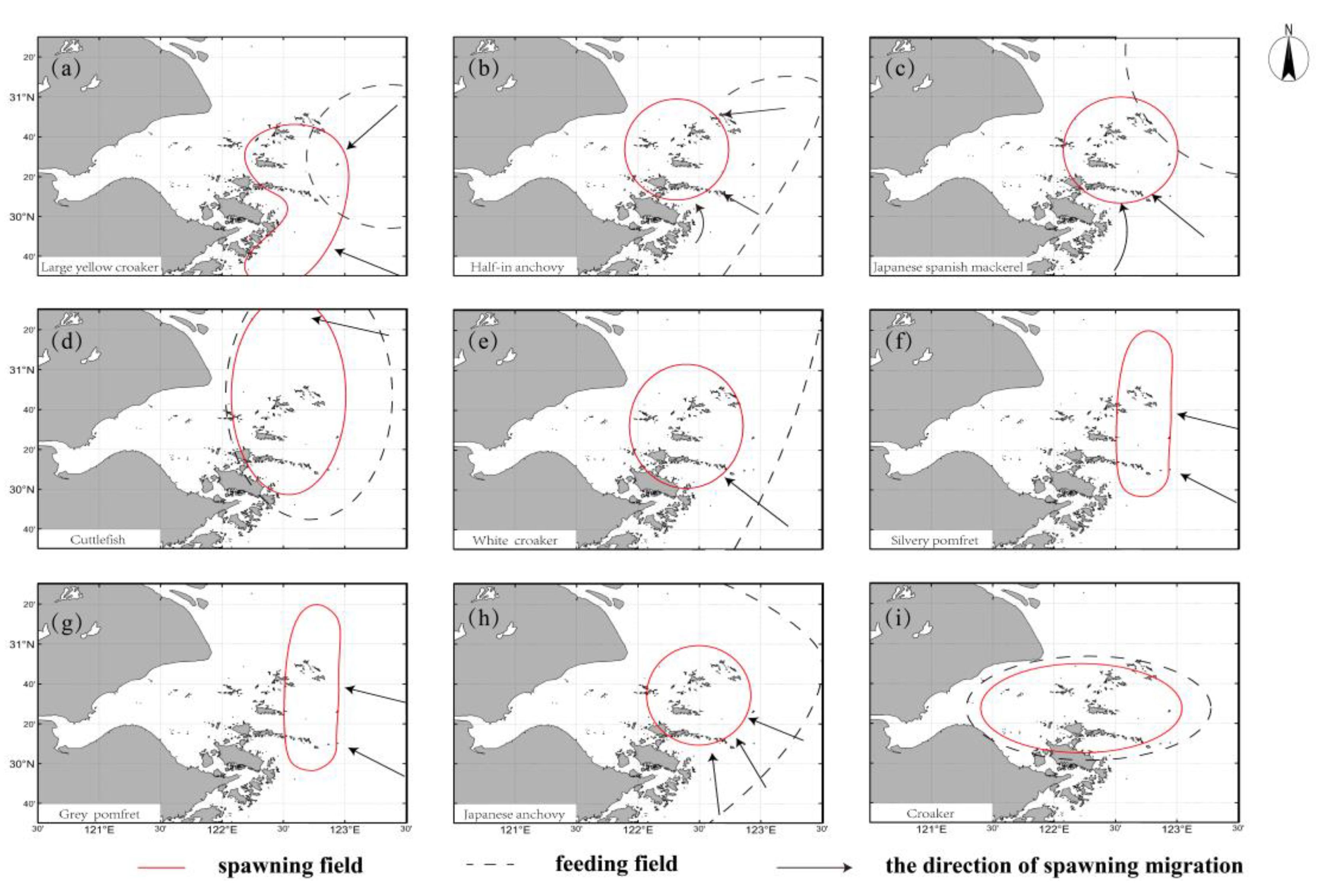
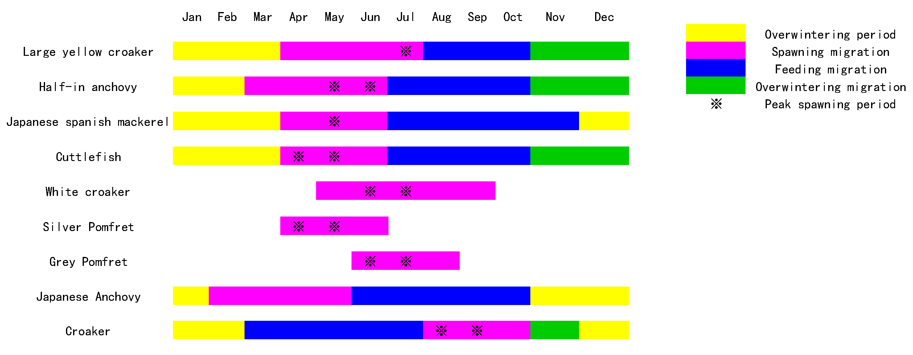
3.5. Distribution of Fishery Resources in the Waters of Zhoushan Archipelago

The study area is rich in fishery resources and is a typical spawning ground and feeding ground. The environmental elements are the foundation of fisheries; therefore, the comparative study was performed between the fishery resources distribution data and chlorophyll concentration to reveal the relationship between the temporal and spatial changes of Chl-a concentration and fishery resources.

In this paper, nine species, including large yellow croaker, half-in anchovy and Japanese Spanish mackerel, etc., which have been the main economical species in the Zhoushan Fishery, and their spawning ground and feeding ground were analyzed (Figure 6 and Figure 7).

Half-in anchovy (Figure 6b), Japanese Spanish mackerel (Figure 6c), white croaker (Figure 6e) and Japanese anchovy (Figure 6h) spawn in the Qushan-island-centered waters (122–123°E, 30–31°N). Cuttlefish (Figure 6d), silvery pomfret (Figure 6f) and gray pomfret (Figure 6g) spawn in the long strip area from 30 to 31.5°N, although the silver and gray pomfrets distribute from 122.3 to 123°E, while the cuttlefish distribute from 122 to 123°E. Large yellow croaker mainly spawns in the Daiquyang waters (Figure 1) (122–123°E, 29.5–30.5°N), and the croaker’s feeding ground is basically the entire Hangzhou Bay (Figure 6i) (121.2–123°E, 30–31°N). The feeding ground of the fish mentioned in this paper is basically the outer 123°E, except for the cuttlefish and croaker, whose feeding ground is basically their spawning ground (Figure 6).

April and May are the peak spawning periods for half-in anchovy, Japanese Spanish mackerel, cuttlefish and silver pomfret. June and July are the peak spawning periods for large yellow croaker, half-in anchovy, white croaker and gray pomfret. August and September are the peak spawning periods for croaker (Figure 7). Basically, the fish start their spawning migration from March, swimming from their overwintering field to the spawning ground. After finishing spawning in July—apart from some species, such as white croaker, which finishes in September, and gray pomfret, which finishes in August—they start the feeding migration. The spawning period of most kinds of fish is May and June (Figure 7), during which a great number of fish might migrate to the Zhoushan islands area to lay eggs; the brood stock and few hatched offspring consume bait, making the Chl-a concentration in this period drop slightly. When it comes to July and August, the fish migrate to the feeding area, which is mostly outside of the study area; after finishing reproduction, the Chl-a concentration rebounds. This is consistent with the conclusions of previous studies [41].

Generally, the Chl-a concentration in the spring, autumn and summer is relatively higher than in the winter, which coincides with the peak of the spawning period for most fish species in the study area.

4. Discussion

4.1. Feasibility of the New Model

Water spectral characteristics change with the change of the Chl-a concentration, as well as other water components. Compared with other ground objects, the reflectivity of water is relatively low, especially for clean water. The spectral curve of the water shows that clean water has obvious absorption in all bands, except for the blue and green band, which shows some reflectance, and the absorption in the near-infrared band is particularly strong [42]. Chl-a has unique reflection spectrum characteristics. The absorption peaks appear at 440 nm and 678 nm wavelength [43]; therefore, waters with different Chl-a concentrations have different spectral characteristics. Chl-a mainly exists in algae. With the increase in Chl-a concentration, the spectral characteristic of water changes, and the absorption in all wavelengths increases. An absorption valley appeared at 560 nm, which is due to the weak absorption of Chl-a and carotene, as well as the scattering of cells at this band. Around 450 nm, 660 nm and 700 nm, an absorption peak appeared, which resulted from the absorption of light by Chl-a [44,45]. Therefore, Chl-a concentration can be estimated based on the Rrs at different wavelengths [46].

However, in turbid waters, the spectral curve will change due to the spectral interference of other substances. Among them, three elements of the water color, including TSM, Chl-a, CDOM, are the most influential factors [47].

The water of the Zhoushan archipelago is typical case II water, with a high concentration of TSM [48], which leads to the normal green–blue band combination model no longer being suitable [49]. Based on the change of the spectral reflectance value obtained from the CZI, we analyzed the sensitivity of bands 1–4 of the CZI data to the in situ Chl-a concentration.

Earlier research found that when constructing the Chl-a concentration inversion model, the accuracy of the model obtained by a combination of different bands is higher than that of the model constructed by a single band [49]. Therefore, we applied the band combination to construct the Chl-a inversion model. In addition, previous studies have pointed out that the increase in suspended sediment concentration will make the estimated value of Chl-a concentration higher, so it is necessary to add a suspended sediment correction factor based on the blue–green band [13]. In this paper, we used the power function of the ratio of the red and green bands (central wavelengths about 650 nm and 560 nm, respectively) as the correction factor of suspended sediment to reduce the influence of suspended sediment and improve the accuracy.

In this article, we combined the in situ data with the Rrs and analyzed the correlation of the single band and multi-band combination, respectively, and finally found the regression equation with the greatest correlation. The execution error analysis of the results confirmed the feasibility of this empirical model.

Previous studies show that the Chl-a concentration over the four seasons in the waters of the Zhoushan archipelago is significantly different. The Chl-a concentration is relatively high in the summer and lower in the winter, and compared to the interior of the bay, the concentration is lower in the eastern part of the Hangzhou Bay near the East China Sea all year round. Our modeled results show good agreement with previous studies [40,50].

4.2. Factors Affecting Chl-a Concentration and the Fishery Resources in the Waters of Zhoushan Archipelago

Many factors in study area can affect the distribution of Chl-a, such as SST, current and wind [51]. Meanwhile, the intensive islands in the waters of the Zhoushan archipelago cause a complex hydrological environment, which can also influence the distribution of Chl-a, as well as the fishery resources [52].

The temperature and the vertical convection of water caused by seasonal wind are two important factors affecting the distribution of Chl-a in the waters of the Zhoushan archipelago [53]. Therefore, Figure 8 was plotted to show the change of sea temperature and wind field in the four seasons in the study area. SST is about 10–16 °C in the winter (Figure 8(1)), and it is much higher in the east than in the nearshore [54]. Winter’s low SST, together with the northern wind (Figure 8(5)) and lack of surface nutrients cause a negative impact on the growth of the phytoplankton, resulting in a decrease in seasonal Chl-a concentration change in the waters of the Zhoushan archipelago [55], with the Chl-a value around 1.5~2.5 μg/L. The SST in the spring is about 13–17 °C (Figure 8(2)). The average summer temperature is about 25 to 30 °C (Figure 8(3)), which is slightly cooler than the surrounding waters due to the upwelling induced by a southern wind. The cold-water masses at the bottom of the East China Sea form a thermocline [56], in addition to the troposphere caused by the southerly wind (Figure 8(7)), enhancing convection and better water mixing [57], which lead to a lower temperature around the islands, making the Chl-a concentration in the summer the highest, with a value up to around 5 μg/L. Moreover, due to the shallow water and strong fusion, coastal waters provide a suitable environment for the growth of the phytoplankton [58], resulting in a higher coastal Chl-a concentration, while it gradually decreases in the outer sea. In the autumn, the SST decreases. At this time, due to the weakened upwelling, the temperature difference with the surrounding sea is reduced, with the average temperature in the autumn of about 20 to 25 °C (Figure 8(4)), and the strengthening of northerly gusts (Figure 8(8)) causing the convection to weaken and the concentration of Chl-a to decrease [59], with a value of around 2–3.5 μg/L.

There are numerous islands in the area of the Zhoushan waters, and they are shaped differently, making their impact on the environment complicated. The upstream side of the island will generate upwelling, which will promote the vertical exchange of the waters near the island, thereby speeding up the circulation rate of nutrients [60,61], which contributes to the increase in Chl-a. In the downstream area of the island, there is a common increase in Chl-a (Figure 6). In addition, with these islands inducing various currents, the waters around the islands exchange fully. This makes the islands’ surrounding area an ideal nutrient operating environment and also provides selectable water conditions, such as shelters, feeding ground or breeding ground, for different types of fish, thus affecting the proliferation of the fishery resources [62]. When studying the topographic control peaks of the ocean, researchers found that the back flow of the islands will generate back eddy currents and vortex streets, resulting in the generation of a negative pressure zone, which will stagnate the TSM and nutrients, and thus attracting the fish to gather [63]. When investigating the fish group by telemetry, the Chinese scientist Jinan Feng drew a similar conclusion [61].

Affected by its location, the fluctuations and tidal currents in the waters of the Zhoushan archipelago are complex. Taking the Shengsi island as an example, during the flooding period, the outer sea tide comes from the southeast, which is the location of Huangzeyang. The tide splits into two tidal currents; one flows around the Gouqi Island to the northwest, and the other flows north, into the waterway between the Gouqi Island and Ma’anshan Island. The Shengsi area is simultaneously affected by these two currents when the tide is rising. The ebb current mainly comes from the ebb tide of the Hangzhou Bay. The topography affects the current, making its discharge into the outer waters relatively strong. This mainly affects the flow condition, and the ebb flows south–southeast [28].

The nutrients brought by the rivers and currents sink with the TSM; thus, the bottom of the water contains high nutrients. When the currents flow, they scour and induce the resuspension of nutrients. The currents stir the lower layer of the water and bring the nutrients into the surface, thus making the primary and secondary productivity increase [1], which contributes to the fishery.

5. Conclusions

Chinese ocean color satellites HY-1C/D CZI data, with a spatial resolution of 50 m, were first applied to observe the Chl-a concentration change in detail in the waters of the Zhoushan archipelago. A new Chl-a inversion model was established based on the ratio of red, green and blue bands of the HY-1C/D CZI data. Chl-a distribution was revealed in detail using the newly built model.

Chl-a concentration in the Zhoushan islands waters had obvious regional and seasonal characteristics. The Chl-a concentration was mainly in the range of 0.5~6 μg/L. High Chl-a area distributed in the west side of the study area, with a value of 3.5~5.5 μg/L. The Chl-a concentration in the east side of the study area was relatively lower, with a value of 0.5~2 μg/L. Chl-a around the islands was higher than in the area far away from the islands. In addition, Chl-a changed with the change of the tidal current. In the islands’ intensive waters, where the currents are complex, Chl-a became higher. Chl-a concentration downstream of the island increased obviously, forming a high Chl-a concentration belt. From a seasonal aspect, Chl-a concentration was highest in the summer and lowest in the winter.

The waters of the Zhoushan archipelago are a spawning ground for many kinds of economic fish, including the large yellow croaker, half-in anchovy and Japanese Spanish mackerel. The peak period of their spawn and the location of their spawning ground are consistent with the spatial-temporal variation of Chl-a. The distribution of the Chl-a can help us predict the location of the spawning ground. The intensive islands, together with other environment factors, such as the tide, SST, wind, current and topography, jointly contribute to the formation of the fishery, affecting the Chl-a concentration and the fish resources.

This is the first time that a suitable Chl-a concentration model was established in the waters of the Zhoushan archipelago based on HY-1C/D CZI data, which can provide a good technical support for the development and environmental monitoring of the islands’ intensive fishery. HY-1C/D satellites have a good potential for monitoring the water quality detail of nearshore waters.

References

1. Ning, X.; Liu, Z.; Hu, Q. Distribution characteristics of chlorophyll a and primary productivity in the upwelling area along the Zhejiang coast. Acta Oceanol. Sin. 1988, 6, 78–82. [Google Scholar]
2. Li, S.; Chen, Z.; Mao, X.; Pan, D. Laboratory Chlorophyll a Concentration Determination. Mar. Environ. Sci. 1988, 2, 78–82. [Google Scholar]
3. Kattawar, G.W.; Humphreys, T.J. Remote sensing of chlorophyll in an atmosphere-ocean environment: A theoretical study. Appl. Opt. 1976, 15, 273–282. [Google Scholar] [CrossRef]
4. Lesht, B.M.; Barbiero, R.P.; Warren, G.J. Verification of a simple band ratio algorithm for retrieving Great Lakes open water surface chlorophyll concentrations from satellite observations. J. Great Lakes Res. 2016, 42, 448–454. [Google Scholar] [CrossRef]
5. Ahn, Y.-H.; Shanmugam, P. Derivation and analysis of the fluorescence algorithms to estimate phytoplankton pigment concentrations in optically complex coastal waters. J. Opt. A Pure Appl. Opt. J. Eur. Opt. Soc. 2007, 9, 352–362. [Google Scholar] [CrossRef]
6. Liu, G.; Li, L.; Song, K.; Li, Y.; Lyu, H.; Wen, Z.; Fang, C.; Bi, S.; Sun, X.; Wang, Z.; et al. An OLCI-based algorithm for semi-empirically partitioning absorption coefficient and estimating chlorophyll a concentration in various turbid case-2 waters. Remote Sens. Environ. 2020, 239, 648–661. [Google Scholar] [CrossRef]
7. Muralikrishna, I.V. Ocean chlorophyll retrieval algorithms. Pergamon 1984, 4, 149–153. [Google Scholar] [CrossRef]
8. Tilstone, G.H.; Angel-Benavides, I.M.; Pradhan, Y.; Shutler, J.D.; Groom, S.; Sathyendranath, S. An assessment of chlorophyll-a algorithms available for SeaWiFS in coastal and open areas of the Bay of Bengal and Arabian Sea. Remote Sens. Environ. 2011, 115, 2277–2291. [Google Scholar] [CrossRef]
9. Rainey, M.P.; Tyler, A.N.; Gilvear, D.J.; Bryant, R.G.; McDonald, P. Mapping intertidal estuarine sediment grain size distributions through airborne remote sensing. Remote Sens. Environ. 2003, 86, 480–490. [Google Scholar] [CrossRef]
10. Zunbin, L.; Deyong, S.; Shengqiang, W.; Zhongfeng, Q.; Yu, H.; Zhihua, M.; Yijun, H. Remote sensing estimation of colored dissolved organic matter (CDOM) from GOCI measurements in the Bohai Sea and Yellow Sea. Environ. Sci. Pollut. Res. Int. 2020, 27, 6872–6885. [Google Scholar]
11. Gitelson, A.A.; Kondratyev, K.Y. Optical models of mesotrophic and eutrophic water bodies. Int. J. Remote Sens. 1991, 12, 373–385. [Google Scholar] [CrossRef]
12. Tassan, S. local algorithms using SeaWifS data for the retrieval of phytoplankton, pigments, suspended sediment, and yellow substance in coastal waters. Appl. Opt. 1994, 33, 2369–2379. [Google Scholar] [CrossRef] [PubMed]
13. Tang, J.; Wang, S.; Song, Q.; Li, T.; Huang, H.; Ren, J.; Jan, W. Statistical inversion model of water color elements in the second-class water bodies in the Yellow and East China Sea. In Proceedings of the 14th National Remote Sensing Technology Academic Exchange Conference, Qingdao, China, 1 October 2003; p. 7. [Google Scholar]
14. Zhao, M.; Li, Y.; Zhang, L.; Cui, C.; Zhu, X. Preliminary Study on Ocean Color Data Derived from Geostationary Ocean Color Satellite:GOCI in Bohai Sea and Yellow Sea; Shanghai Pujiang Education Press: Shanghai, China, 2015; pp. 661–672. [Google Scholar]
15. Yapa, K.K.A.S. Seasonal variability of sea surface chlorophyll-a of waters around Sri Lanka. J. Earth Syst. Sci. 2000, 109, 427–432. [Google Scholar] [CrossRef]
16. Pinkerton, M.H.; Richardson, K.M.; Boyd, P.W.; Gall, M.P.; Zeldis, J.; Oliver, M.D.; Murphy, R.J. Intercomparison of ocean colour band-ratio algorithms for chlorophyll concentration in the Subtropical Front east of New Zealand. Remote Sens. Environ. 2005, 97, 382–402. [Google Scholar] [CrossRef]
17. Prakash, P.; Kumar, T.S.; Rahman, S.H.; Nayak, S. Binning algorithm for high-resolution IRS-P4 OCM chlorophyll image. Int. J. Remote Sens. 2012, 33, 5789–5798. [Google Scholar] [CrossRef]
18. Pittman, N.A.; Strutton, P.G.; Johnson, R.; Matear, R.J. An Assessment and Improvement of Satellite Ocean Color Algorithms for the Tropical Pacific Ocean. J. Geophys. Res. Ocean. 2019, 124, 9020–9039. [Google Scholar] [CrossRef]
19. Matthews, M.W.; Odermatt, D. Improved algorithm for routine monitoring of cyanobacteria and eutrophication in inland and near-coastal waters. Remote Sens. Environ. 2015, 156, 374–382. [Google Scholar] [CrossRef]
20. Dekker, A.G.; Vos, R.J.; Peters, S.W.M. Analytical algorithms for lake water TSM estimation for retrospective analyses of TM and SPOT sensor data. Int. J. Remote Sens. 2002, 23, 15–35. [Google Scholar] [CrossRef]
21. Zou, Y. Analysis of Temporal and Spatial Distribution Characteristics of Chlorophyll a in Bohai Sea. Remote Sens. Inf. 2004, 12, 30–31, 62. [Google Scholar]
22. Zhou, L.; Chen, J.; Sun, J.; Fu, J. Monitoring seasonal distribution of chlorophyll a concentration in Taihu Lake based on CBERS-1 images. Spectrosc. Spectr. Anal. 2011, 31, 530–534. [Google Scholar]
23. Guo, Y.; Qian, J.; Lei, Y.; Dong, S.; Wu, C.; Qu, W.; Zhang, Q. Joint inversion of chlorophyll a concentration in reservoirs based on GF-1 satellite data. Surv. Eng. 2021, 30, 14–19. [Google Scholar]
24. Fan, D.-X.; Huang, Y.-L.; Song, L.-X.; Liu, D.-F.; Zhang, G.; Zhang, B. Prediction of chlorophyll a concentration using HJ-1 satellite imagery for Xiangxi Bay in Three Gorges Reservoir. Water Sci. Eng. 2014, 7, 70–80. [Google Scholar]
25. Shanmugam, P. A new bio-optical algorithm for the remote sensing of algal blooms in complex ocean waters. J. Geophys. Res. Earth Surf. 2011, 116, 16–40. [Google Scholar] [CrossRef]
26. O’Reilly, J.E.; Werdell, P.J. Chlorophyll algorithms for ocean color sensorsOC4, OC5 & OC6. Remote Sens. Environ. 2019, 229, 32–47. [Google Scholar]
27. Feng, L. Shengsi, Zhejiang: Constructing Marine Ranch to Conserve “Blue Land”. Chin. Land 2019, 3, 56–57. [Google Scholar]
28. Li, Y.; Miao, Z. Analysis of hydrological characteristics of squid spawning grounds in northern Zhejiang. J. Zhejiang Fish. Inst. 1986, 2, 139–145. [Google Scholar]
29. Song, Y. Hydrological characteristics of Zhoushan Islands. Hydrology 2001, 1, 59–62. [Google Scholar]
30. Liu, L.; Sui, Y.; Jiang, R.; Xu, K.; Zhu, W.; Zhou, Y. Species composition and quantity distribution of eggs, larvae and juveniles in Zhoushan fishery in spring. J. Zhejiang Ocean Univ. (Nat. Sci. Ed.) 2021, 40, 1–8. [Google Scholar]
31. Cai, L.; Tang, D.; Li, X.; Zheng, H.; Shao, W. Remote sensing of spatial-temporal distribution of suspended sediment and analysis of related environmental factors in Hangzhou Bay, China. Remote Sens. Lett. 2015, 6, 597–603. [Google Scholar] [CrossRef]
32. Yu, C.; Chen, Q.; Chen, X.; Ning, P.; Zheng, J. Composition and quantity distribution of fish species in Zhoushan fishery and adjacent waters. Oceanol. Limnol. Sin. 2010, 41, 410–417. [Google Scholar]
33. Li, T.; Wang, Y.; Jin, Y.; Hu, H. Interannual variation of nutrient content and degree of eutrophication in Daiquyang from 2011 to 2017. In Proceedings of the 2nd International Symposium on Modern Marine Ranching, 2018 Academic Annual Meeting of Fishery Resources and Environment Professional Committee of Chinese Fisheries Society, Dalian, China, 28–30 October 2018; p. 1. [Google Scholar]
34. “Ocean Survey Specifications” series of national standards. Stand. China 2011, 2, 22–23.
35. An unstructured grid, finite-volumn coastal ocean model (FVCOM) system. Oceanography 2006, 6, 19.
36. Chen, C.; Xue, P.; Ding, P.; Beardsley, R.C.; Xu, Q.; Mao, X.; Gao, G.; Qi, J.; Li, C.; Lin, H.; et al. Physical mechanisms for the offshore detachment of Changjiang diluted water in the East China Sea. J. Geophys. Res. 2008, 113, 122–125. [Google Scholar] [CrossRef]
37. Chen, X.-Y.; Zhang, J.; Tong, C.; Liu, R.-J.; Mu, B.; Ding, J. Retrieval Algorithm of Chlorophyll-a Concentration in Turbid Waters from Satellite HY-1C Coastal Zone Imager Data. J. Coast. Res. 2019, 90, 146–155. [Google Scholar] [CrossRef]
38. Tong, C.; Mu, B.; Liu, R.-J.; Ding, J.; Zhang, M.-W.; Xiao, Y.-F.; Liang, X.-J.; Chen, X.-Y. Atmospheric Correction Algorithm for HY-1C CZI over Turbid Waters. J. Coast. Res. 2019, 90, 156–163. [Google Scholar] [CrossRef]
39. Zhang, X.; Zheng, X. Comparison of inversion algorithms for chlorophyll concentration in Bohai Bay based on GOCI data. Mar. Sci. Bull. 2017, 19, 62–74. [Google Scholar]
40. Zhang, J.; Shen, F.; Yu, X.; Zhou, Y. Winter and summer variation of phytoplankton absorption characteristics in the adjacent waters of Hangzhou Bay. Geogr. Geo-Inf. Sci. 2013, 29, 112–118. [Google Scholar]
41. Fu, J.; Chen, C.; Chu, Y. Spatial–temporal variations of oceanographic parameters in the Zhoushan sea area of the East China Sea based on remote sensing datasets. Reg. Stud. Mar. Sci. 2019, 28, 100626. [Google Scholar] [CrossRef]
42. Harish, C.M.; Baba, M. On spectral and statistical characteristics of shallow water waves. Pergamon 1986, 13, 239–248. [Google Scholar] [CrossRef]
43. Oba, T.; Mimuro, M.; Wang, Z.Y.; Nozawa, T.; Yoshida, S.; Watanabe, T. ChemInform Abstract: Spectral Characteristics and Colloidal Properties of Chlorophyll a′ in Aqueous Methanol. ChemInform 1997, 28, 99–113. [Google Scholar] [CrossRef]
44. Tian, G.; Mi, X.; Song, F.; Zhao, W. Estimation of Chlorophyll Concentration in Water Using Spectral Dat. Environ. Remote Sens. 1988, 1, 71–80. [Google Scholar]
45. Lin, S.; Wu, Q.; Wang, X.; Pu, X.; Dai, Y. The relationship between chlorophyll content of phytoplankton in Chaohu Lake and the characteristics of reflectance spectrum. J. Lake Sci. 2002, 228–234. [Google Scholar]
46. Lin, Y.; Ye, Z.; Zhang, Y.; Yu, J. Spectral feature analysis for quantitative estimation of cyabobacteria chlorophyll-a. ISPRS Int. Arch. Photogramm. Remote Sens. Spat. Inf. Sci. 2016, 91, XLI-B7. [Google Scholar]
47. Liu, X.; Li, T.; Chen, Q. The influence of the main components of water body on the apparent chemometrics. Mar. Technol. 2004, 1, 85–89. [Google Scholar]
48. Shuyi, H.; Jianqiang, L.; Lina, C.; Minrui, Z.; Juan, B.; Jieni, X. Satellites HY-1C and Landsat 8 Combined to Observe the Influence of Bridge on Sea Surface Temperature and Suspended Sediment Concentration in Hangzhou Bay, China. Water 2020, 12, 2595. [Google Scholar]
49. Menon, H.B.; Adhikari, A. Remote Sensing of Chlorophyll-A in Case II Waters: A Novel Approach With Improved Accuracy Over Widely Implemented Turbid Water Indices. J. Geophys. Res. Ocean. 2018, 123, 8138–8158. [Google Scholar] [CrossRef]
50. Liu, Z.; Ning, X.; Cai, Y. Phytoplankton existing stock and primary productivity in autumn in Hangzhou Bay-Zhoushan fishery. Chin. J. Oceanogr. (Chin. Version) 2001, 2, 93–99. [Google Scholar]
51. Çulha, S.T.; Karaduman, F.R. The influence of marine fish farming on water and sediment quality: Ildır Bay (Aegean Sea). Environ. Monit. Assess. 2020, 192, 528–537. [Google Scholar] [CrossRef]
52. Russ, G.R.; Rizzari, J.R.; Abesamis, R.A.; Alcala, A.C. Coral cover a stronger driver of reef fish trophic biomass than fishing. Ecol. Appl. A Publ. Ecol. Soc. Am. 2020, 31, 21–43. [Google Scholar] [CrossRef]
53. Ji, C.; Zhang, Y.; Cheng, Q.; Tsou, J.; Jiang, T.; Liang, X.S. Evaluating the impact of sea surface temperature (SST) on spatial distribution of chlorophyll-a concentration in the East China Sea. Int. J. Appl. Earth Obs. Geoinf. ITC J. 2018, 68, 252–261. [Google Scholar] [CrossRef]
54. Jiang, S.; Wang, Y.; Ma, R. Variation analysis of chlorophyll concentration in East China Sea and its response to seawater temperature. Bull. Surv. Mapp. 2020, 6, 39–44. [Google Scholar]
55. Tae, J.S.; Hak, L.J.; Ho, K.C.; Joo, J.C.; Suk, J.Y. Movement of Cold Water Mass in the Northern East China Sea in Summer. Sea 2011, 16, 1–13. [Google Scholar]
56. Liu, X.; Hou, Y.; Yin, D.; Yang, S. Dynamics of circulation, temperature and salt structure in the Yangtze Estuary and its adjacent sea area Ⅲ Temperature structure. Oceanol. Limnol. Sin. 2015, 46, 526–533. [Google Scholar]
57. Ma, B.; Zhao, H. Distribution characteristics of chlorophyll a and nutrients in the Pearl River Estuary in summer and their relationship with environmental factors. Mar. Environ. Sci. 2021, 40, 707–716. [Google Scholar]
58. Zhu, J. Dynamic mechanism of the upwelling on the west side of the submerged river valley off the Changjiang mouth in summertime. Chin. Sci. Bull. 2003, 48, 2754–2758. [Google Scholar] [CrossRef]
59. Li, W.; Wang, Z.; Huang, H. Relationship between the southern Yellow Sea Cold Water Mass and the distribution and composition of suspended particulate matter in summer and autumn seasons. J. Sea Res. 2019, 154, 101812–101827. [Google Scholar] [CrossRef]
60. Seaman, W. Artificial Reef Evaluation:With Application to Natural Marine Habitats; CRC Press: Boca Raton, FL, USA, 2000. [Google Scholar]
61. Feng, J.; Wang, Y. Reefs and bioenvironments—fish distribution and activity in reef fisheries. Aquat. Technol. 2002, 3, 22–24. [Google Scholar]
62. Wang, H.; Chen, P.; Zhang, S.; Jia, X. Effects of artificial reefs on the proliferation of fishery resources. Guangdong Agric. Sci. 2009, 8, 18–21. [Google Scholar]
63. Wolanski, E.; Hamner, W.M. Topographically controlled fronts in the ocean and their biological influence. Science 1988, 241, 177–181. [Google Scholar] [CrossRef]
Figure 1. (a): Location of Hangzhou Bay, Black square in (a): Hangzhou Bay. (b): Shengsi and its surroundings. (c): The water depth topographic map of Hangzhou Bay, in which the black square represents the study area.
Remotesensing 14 04270 g001
Figure 2. Distribution of sampling sites. The red square: the distribution of sampling points for the data used in this paper.
Remotesensing 14 04270 g002
Figure 3. Correlation between band reflectance and natural logarithm of the sampled Chl-a concentration. (ad): The linear relationship between the Rrs of band 1, 2, 3, 4 and natural logarithm of the sampled Chl-a concentration. The abscissa is the value obtained after atmospheric correction, and the ordinate is the value of in situ Chl-a concentration.
Remotesensing 14 04270 g003
Figure 4. Comparison of modeled Chl-a concentration value and in situ Chl-a value.
Remotesensing 14 04270 g004
Figure 5. The distribution of Chl-a in the waters of Zhoushan archipelago from 2019 to 2021. (115): Chl-a retrieved from CZI loaded in HY-1C. (1630): Chl-a retrieved from CZI loaded in HY-1 D. Black arrow: the direction of the local currents. Red circles: the obvious wakes induced by islands.
Remotesensing 14 04270 g005
Figure 6. (ai) The spawning grounds and feeding grounds of nine main fish species, including Large yellow croaker, half-in anchovy, Japanese Spanish mackerel, cuttlefish, white croaker, silvery pomfret, grey pomfret, Japanese anchovy and croaker. Red circle: The spawning ground. Dotted line: The feeding ground. Arrows: The direction of spawning migration.
Remotesensing 14 04270 g006
Figure 7. The growth period of nine main fish species in the study area.
Remotesensing 14 04270 g007
Figure 8. (14) Average SST of winter, spring, summer, autumn. (58) Wind of the corresponding month in Hangzhou Bay. (912): The Chl-a concentration in the representative days of four seasons in island intensive area.
Remotesensing 14 04270 g008