
An Analysis of the Optimal Features for Sentinel-1 Oil Spill Datasets Based on an Improved J–M/K-Means Algorithm

School of Navigation, Dalian Maritime University, Dalian 116026, China
*
Author to whom correspondence should be addressed.
Remote Sens. 2022, 14(17), 4290; https://0-doi-org.brum.beds.ac.uk/10.3390/rs14174290
Submission received: 28 July 2022
/
Revised: 19 August 2022
/
Accepted: 25 August 2022
/
Published: 31 August 2022
(This article belongs to the Special Issue Advances in Oil Spill Remote Sensing)
Abstract
:With the rapid development of world shipping, oil spill accidents such as tanker collisions, illegal sewage discharges, and oil pipeline ruptures occur frequently. As the SAR system expands from single polarization to multipolarization, the Polarmetric Synthetic Aperture Radar (Pol-SAR) system has been widely used in marine oil spill detection. However, in the studies of the oil spill extraction in SAR images, there are some problems that limit large-scale oil spill detection work. As a transition from single-polarized to full-polarized, the dual-polarized system carries some polarization information and can be obtained in large quantities for free, which has become a major breakthrough in solving the problem of large-scale oil spill detection. In order to optimize the multisource features that can be extracted from dual-polarized SAR images, greatly improve the utilization rate of dual-polarized SAR oil spill images under the premise of reducing workload, and ensure the accuracy of marine oil spill extraction, this paper adopts the metric of inter-class separability, the Jeffries–Matusita distance, which improves on the traditional K-means algorithm by focusing on the noise sensitivity defect of the K-means algorithm; the artificial influence of J–M distance in measuring the separability between classes improves the algorithm in three aspects: sample selection, distance calculation, and data evaluation. Finally, using the inter-sample J–M distance of multisource features, the overall accuracy of image segmentation, the F1-score, and the results of correlation analysis between features, three advantageous features and three subdominant features are selected that can be used for marine oil spill detection.
1. Introduction
The discharge of pollutants into the sea will not only cause marine pollution but also indirectly destroy the marine ecological balance, thus threatening the living environment of marine life and human beings [1]. Marine pollutants mostly include petroleum, heavy metals, organic substances, and radionuclides. As a common pollutant, oil has frequently spilled in various sea areas in recent years, which is closely related to the development of the shipping economy and offshore oil exploration and extraction industries. The distribution of marine oil spills caused by tanker collisions and illegal pollution discharges is mostly related to routes [2]. According to statistics, the amount of oil spilled at sea caused by ships underway can reach about 457,000 tons a year [3]. Among the observed marine oil pollution, oil spills caused by tanker accidents account for only 5% of the total, while the remaining 95% mostly come from illegal pollution discharges [4]. Toxic substances contained in petroleum will exist in seawater for a long time, which will not only cause great harm to the marine ecological environment including the mass deaths of marine organisms but also affect the development of human society and economy [5].
Remote sensing technology has been widely used in the field of marine oil spill detection. Since the rise of Synthetic Aperture Radar (SAR) technology, new breakthroughs have been made in marine oil spill detection. Compared with optical sensors, the polarimetric SAR system works in the microwave range and is not affected by weather or time. Moreover, the SAR images give information based on the principle of scattering, which provides a new basis for the extraction of marine oil spills from images [6]. Extensive research has been carried out on oil spill detection using polarimetric SAR data, but there are still problems such as insufficient available data and low utilization of the information carried by polarimetric SAR data [7]. Existing polarimetric SAR oil spill extraction methods are mostly based on fully polarimetric SAR data. Due to the scarcity and high price of fully polarimetric SAR data, this data source is difficult to apply to long-term and large-scale oil spill detection. In contrast, the dual-polarized SAR connects the single-polarized system and the full-polarized system, which not only carries part of the polarization information but also can be obtained in large quantities, which is more suitable for large-scale oil spill detection. However, there are few applications of dual-polarized SAR in oil spill detection at present, and there is a lack of systematic analysis and evaluation of the oil spill detection characteristics of dual-polarized SAR. Therefore, it is very important to analyze the advantages of multiple oil spill detection features to improve the accuracy and efficiency of dual-polarized SAR oil spill detection.
The polarimetric SAR oil spill detection process consists of two steps: feature selection and image segmentation. In the preprocessing stage of oil spill detection, feature selection seeks the appropriate features that can effectively utilize image information and improve oil spill detection accuracy. Fiscella et al. used only geometric and texture features are involved in their oil spill detection work [8]. Topouzelis et al. used 25 feature parameters including geometric, grayscale, and texture features for oil spill detection [9]. Singha et al. studied oil spill identification based on decision tree theory and introduced 23 geometric features, 5 grayscale features, 8 texture features, and 5 spatial features [10]. It can be seen from the above studies that feature selection is mostly based on five categories [11], namely grayscale, texture, geometry, context, and SAR polarimetry [12]. High-dimensional feature space will theoretically increase the reliability of oil spill detection, but in practical applications, it may cause the algorithm to overload and reduce the detection accuracy. Based on the above five feature categories, researchers screen the dominant features; common methods include correlation, inter-class distance, and information entropy. Skrunes et al. extracted eight commonly used multipolarized features based on the HH–VV dual-polarized images and found that the geometric intensity V and the real part of the cross-polarized product have advantages in oil spill detection [13]. In 2016, Singha et al. compared the differences between polarimetric features and traditional features in oil spill and oil-like spill identification and analysis and identified that geometric strength, co-polarization ratio, and total power are more suitable for oil spill detection [14]. Yu et al. proposed a fast-filtering method (the fast correlation-based filter solution, FCBF) that can effectively identify related features and the redundancy between related features. The results showed that the algorithm is feasible for feature selection for high-dimensional data classification [15]. Peng et al. derived the minimum redundancy maximum correlation criterion (mRMR) based on mutual information and proposed a two-stage feature selection algorithm. The results showed that the introduction of mRMR feature selection can significantly improve the classification accuracy [16].
In addition, machine learning-based dual-polarization SAR oil spill detection is also a major research direction. Using amplitude information and phase information, combined with Cloud decomposition, Ma proposes an intelligent oil spill detection architecture based on a deep convolutional neural network (DCNN) that can better capture oil spills and achieve fine-scale segmentation [17]. Prastyani’s semi-automatic detection of the Balikpapan Gulf oil spill based on Sentinel-1 data demonstrates the potential of Sentinel-1 imagery in oil spill detection [18]. Starting from the nonlocal mean intensity map, intensity texture, and polarization information, Kim proposed an ANN algorithm based on dual-polarization SAR images and achieved good oil spill detection results [19]. However, most of the dual-polarization SAR oil spill detection research based on machine learning starts from the image level and seldom considers the imaging mechanism and unique properties of SAR; additionally, it is difficult to obtain the characteristics that perform well in the process of oil spill detection. Therefore, this study starts from feature selection and uses the J–M distance as a measure to obtain the dominant feature set for Sentinel-1 oil spill data detection.
In this study, 19 multisource features for oil spill detection with dual-polarized SAR were extracted from 3 perspectives, backscatter information, H-α polarimetric decomposition, and grayscale texture, for dominance analysis. In terms of method, this study introduces a measure of separation between classes commonly used in remote sensing image classification, the Jeffries–Matusita distance (hereinafter referred to as J–M distance), to improve the classical image segmentation algorithm K-means. This method replaces the Euclidean distance with the J–M distance, which greatly compensates for the defect that the traditional K-means method is sensitive to noise and outliers. At the same time, the J–M distance between samples is calculated in the process of image segmentation, so that the result of the J–M distance can be more independent of the selection of samples, and the influence of manual intervention is reduced. This paper analyzes 19 multisource features based on the J–M distance and segmentation accuracy, which provides a reference for the selection of oil spill detection features for dual-polarized SAR.
2. Related Studies
2.1. Feature Parameters of Dual-Polarized SAR
The dual-polarized SAR system connects the single-polarized system and the full-polarized system but can only obtain partial polarimetric information [20]. In order to better improve the usability of bipolar data, a total of 19 features are extracted in this paper and will be introduced individually. For the purpose of comprehensively evaluating the dominance of multiple feature pairs in dual-polarized SAR oil spill detection, we extracted 19 features from backscatter information, H-α polarimetric decomposition, and grayscale texture.
The features based on backscattering information include backscattering intensity and combined polarimetric matrix transformation. In the SAR imaging process, the backscattered energy of the VV polarimetric channel on the sea surface is the strongest and is often used as a single-polarized oil spill detection feature. Chaturvedj analyzed polarized SAR oil spill images in the waters between Saudi Arabia and Kuwait with the Persian Gulf as the research area and also proved that the VV polarimetric channel is more suitable for oil spill detection than the cross-polarized channel [21]. Furthermore, by transforming the C2 covariance matrix, characteristic parameters including covariance diagonal element , polarimetric ratio PR, and polarimetric span are extracted. The definition of polarimetric ratio PR and polarimetric span in a dual-polarized SAR system is shown in Formulas (1) and (2):
where and represent the diagonal elements of the covariance matrix and and represent the two eigenvalues.
The polarized SAR system stores the amplitude and phase difference information on the combined echoes of different polarimetric channels in the form of a scattering matrix. In SAR images, the oil film and the background seawater have different scattering mechanisms. Under the same wavelength, the backscattering coefficients of the two are quite different and have obvious contrast. Therefore, the performance of the two in the polarimetric characteristic space also has a certain degree of difference [22]. Starting from eigenvalues and eigenvectors, Cloud constructs the H/α plane, which provides a basis for subsequent feature extraction and scattering characteristic analysis [23]. Based on the H-α polarimetric decomposition, three characteristics, polarization entropy H, anisotropy A, and polarimetric scattering angle α can be obtained. For their detailed definitions, see Equations (3)–(5):
The combined polarimetric parameters preserve the properties of different parameters through mathematical transformation while enhancing the separability between targets, and they are widely used in oil spill detection. On the basis of polarimetric entropy H and anisotropy A, Schuler proposed H_A features according to several mathematical combinations of parameters and achieved good results in oil spill detection. The H_A combined features include , , and [24].
Texture features represent the detailed characteristics of ground objects, reflect the grayscale transformation relationship between pixels, and have a nonnegligible role in distinguishing various targets [25]. The texture feature extraction method based on GLCM (gray level co-occurrence matrix) is more commonly used in SAR oil spill detection. In this study, by obtaining different co-occurrence matrices, a total of eight commonly used texture features including mean, second-order moment, and contrast are extracted for dominance analysis:
- Mean Mean
- Maximum Max
- Variance Varwhere µ is the mean of .
- Contrast Con
- Second-order moment ASM
- Second-order entropy Ent
- Homogeneity Hom
- Dissimilarity Dis
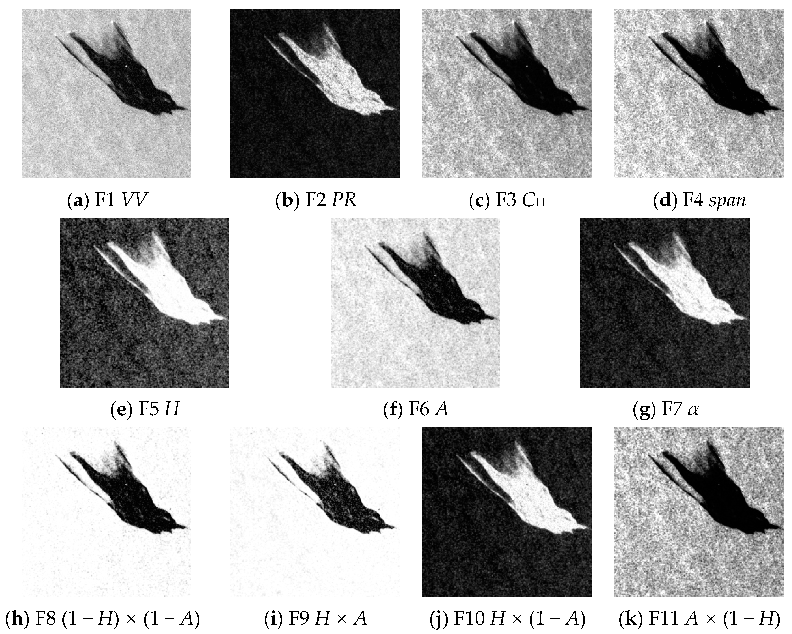
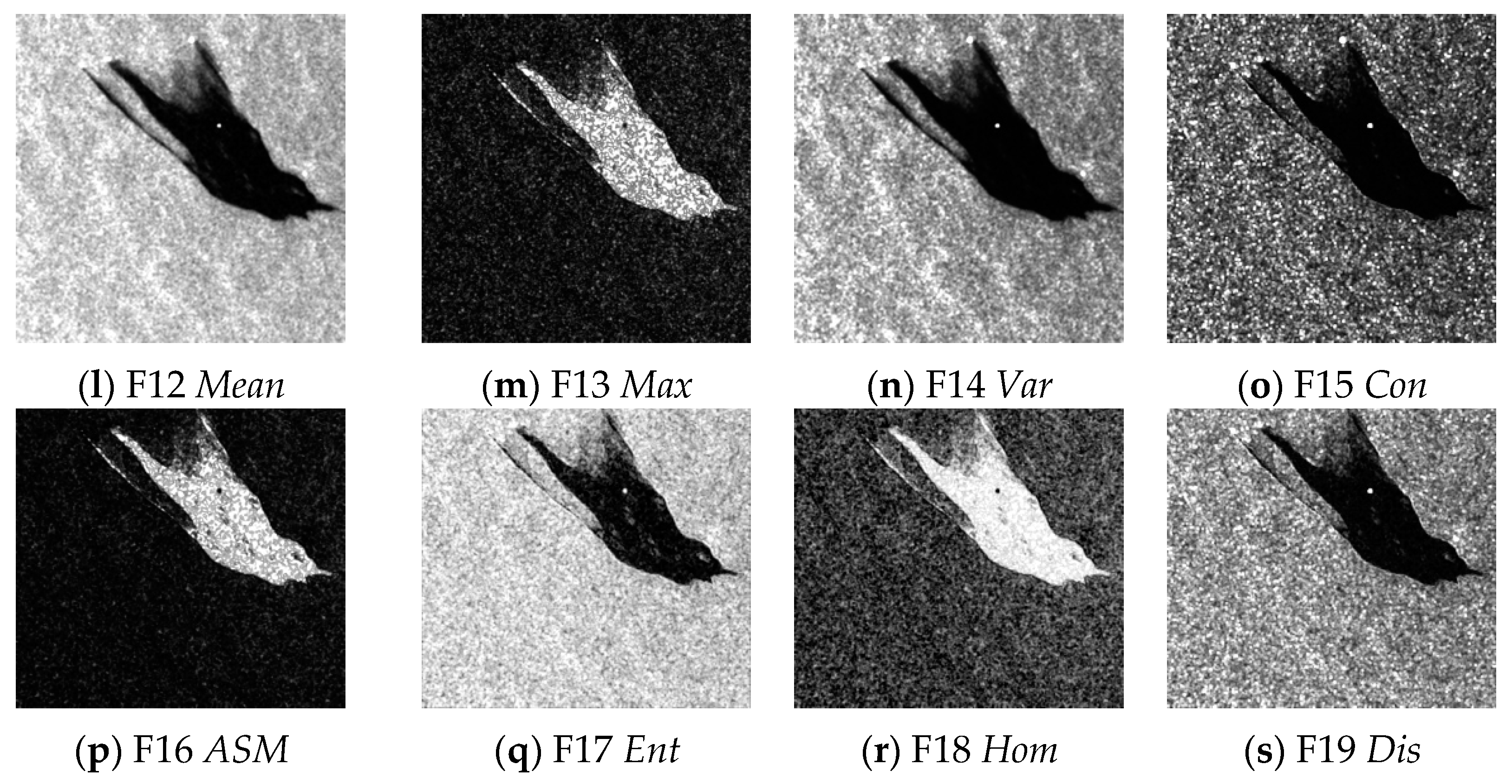
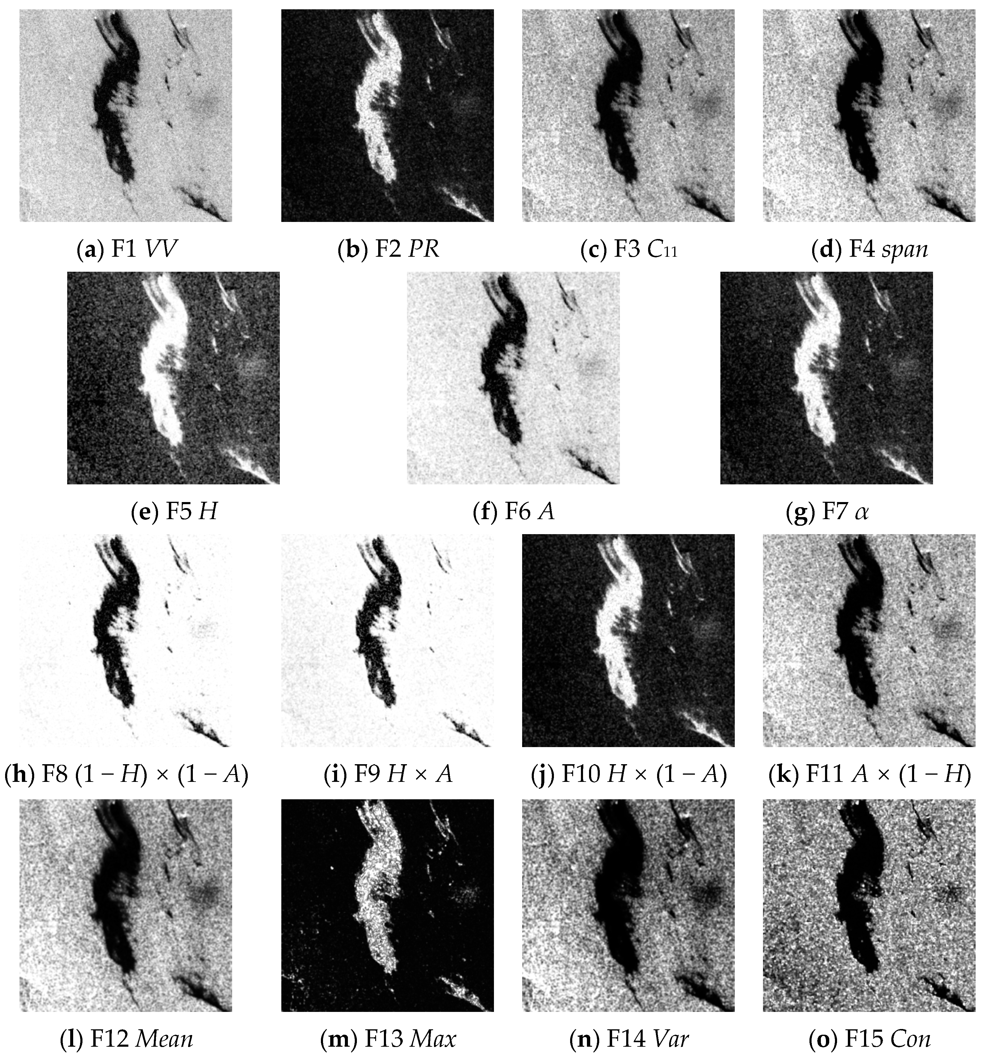
For the convenience of the following descriptions, the 19 oil spill detection features are numbered in Table 1.
2.2. K-Means Clustering Algorithm
The K-means algorithm, also known as the K-means clustering algorithm, is an unsupervised, nondeterministic iterative method that is widely used in large-scale dataset clustering problems [26]. In 1967, MacQueen first proposed the K-means algorithm [27]. The algorithm uses distance as the similarity evaluation index, divides data objects into K different clusters, and iterates until the moving distance of the K cluster centers is less than the given value. Due to this distance-based clustering method, the clustering results generated by the K-means algorithm are compact and independent, and the algorithm is simple, fast, and easy to implement.
The implementation of the algorithm includes two stages. The first stage is to determine the k cluster centers, and the second stage is to divide all data objects into K clusters by iteration [28]. When the criterion function achieves a local minimum, the clustering result is considered to be stable, and the criterion function is defined as follows:
E is the sum of the squared errors of all data objects, x represents the data objects, is the mean vector of the cluster , and the expression for is:
The accuracy of the traditional K-means algorithm will be affected by the number of clusters K, the initial cluster center, and the distribution of samples. In addition, the algorithm has shortcomings such as being sensitive to noise and outliers, which is an unfavorable effect for SAR images containing a large amount of speckle noise and needs to be improved for application.
2.3. Jeffries–Matusita Distance
In remote-sensing image classification problems, adding more observations or parameters to the feature space to better describe the data categories does not necessarily improve classification accuracy [29]. Therefore, it is necessary to measure the separability between samples of different classes. The indicators often used to evaluate the separability of features between different categories include correlation analysis, inter-class distance, and information entropy. Using distance to measure inter-class separation is a simple and easy-to-implement method. Common distance measures include Bavarian distance, Mahalanobis distance, and J–M distance.
The J–M distance is a widely used statistical separability criterion with a value ranging from 0 to 2. The J–M distance takes the class mean and mean distribution as the separability criteria and is realized by the covariance matrix of the class [30]. The J–M distance can be used not only to evaluate the quality of selected samples in the feature space but also as a standard to measure the inter-class separability of features, and it is widely used in remote-sensing image classification problems, especially in high-dimensional feature spaces [31].
The definition of the J–M distance is as follows:
In the formula, represents the Bavarian distance between two categories and , defined as:
and are the conditional probability density functions of the feature X, and the Babbitt distance can also be expressed as in [32]:
In the formula, and represent the pixel value mean of the two categories; and represent the pixel value standard deviation of the two categories.
From the perspective of parameterization, the separability of two categories on a certain feature is approximately related to the J–M distance. When the J–M distance is higher, the separability between the two categories is also greater. Based on a large number of experiments and past research experience, with 1, 1.8, and 1.9 as the demarcation points, the J–M distance can be divided into three types: When the J–M distance is less than 1, the two categories are inseparable in this feature; when the J–M distance is greater than 1 but less than 1.8, the two categories are separable under this feature, but the separability is poor, which may be related to the selected training samples; when the J–M distance is greater than 1.9, the two categories have strong separability under this feature. It can be seen that the J–M distance is easily affected by the selection of samples, and the separability results obtained from using it as a standard have certain uncertainties.
3. Methods
3.1. Improved J–M/K-Means Algorithm
The traditional K-means algorithm uses Euclidean distance as the clustering criterion. Euclidean distance is a commonly used distance definition that represents the true distance between two points in n-dimensional space. The Euclidean distance in two-dimensional space is the distance between two points; the formula is as follows:
The Euclidean distance is simple to calculate and is mostly used to calculate distance measures, but the K-means algorithm based on Euclidean distance has the defect of being sensitive to noise and outliers, and it cannot measure the superiority of different features for oil spill extraction. On the contrary, J–M distance, as a common distance measure to weigh the degree of separation between classes, has a greater advantage than Euclidean distance in the screening of dominant features. However, inter-class separation measurement based on J–M distance is limited by data distribution and sample selection. If the selected training samples are not scientific enough, the optimal feature results based on the J–M distance will hardly be instructive.
Aiming at solving above problems, this paper used J–M distance to replace Euclidean distance, improving the K-means algorithm. In the evaluation process, taking the J–M distance of the feature map and the image segmentation accuracy as the standards, a feature-screening algorithm with better noise suppression effect and measuring the dominance of different features was obtained.
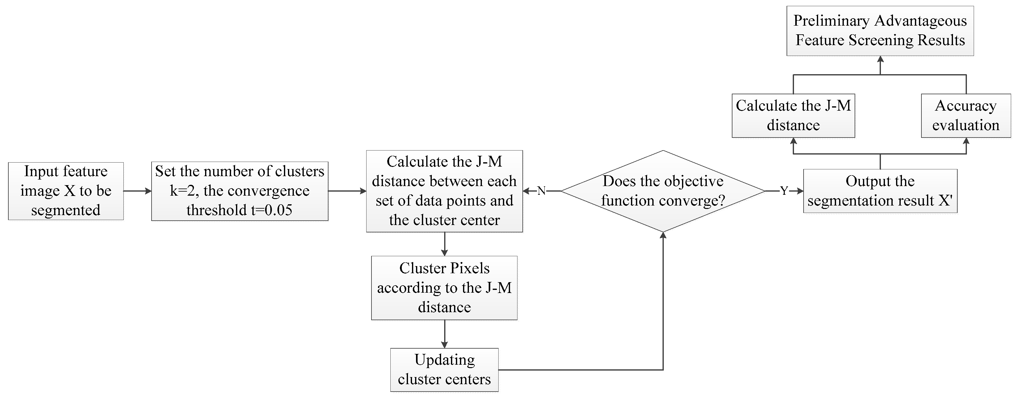
The workflow of the model is shown in Figure 1. The function of each module is discussed.
3.1.1. Selection of Data Point
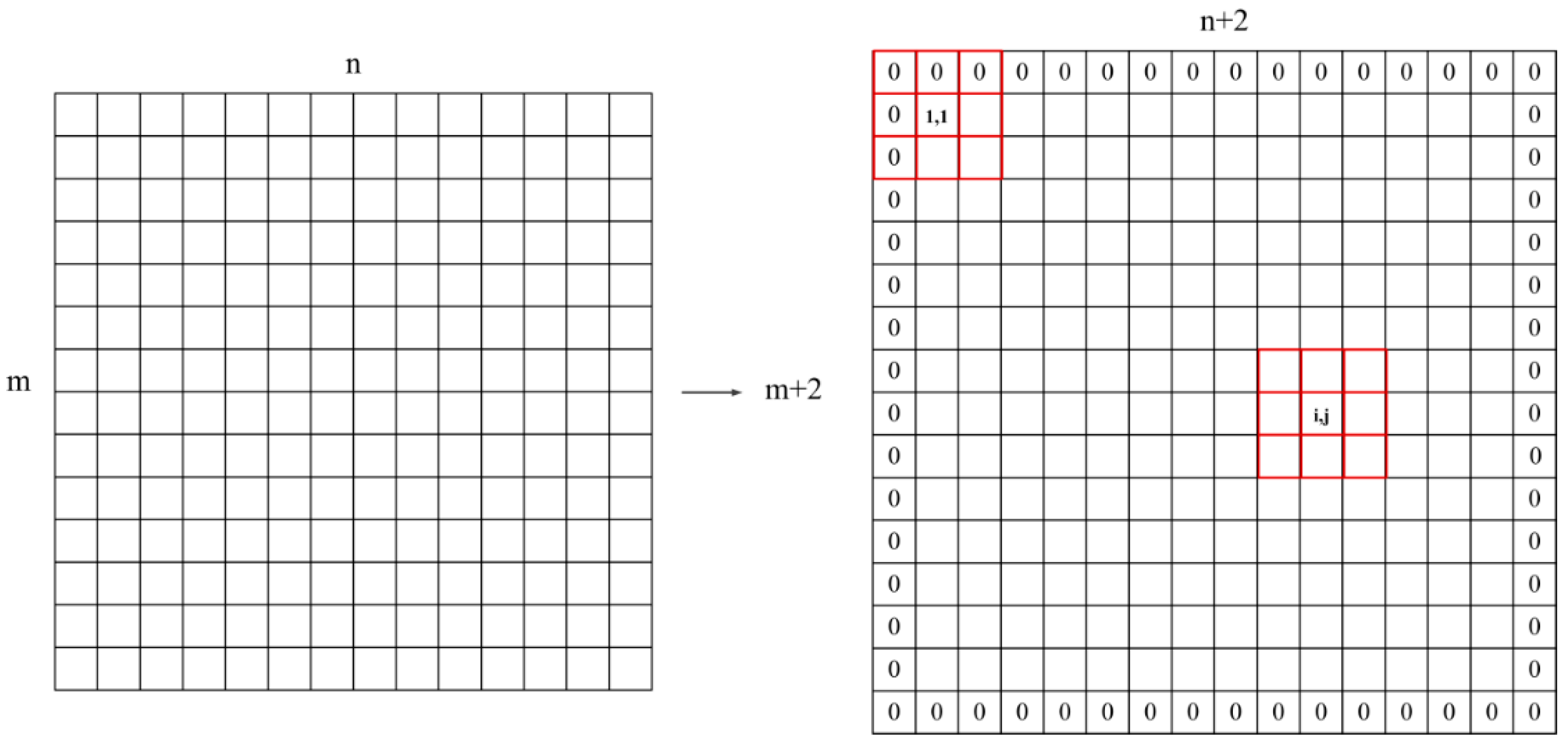
Due to the unique imaging method of the SAR system, polarized SAR images often contain a large amount of speckle noise. In order to make up for the defect that the traditional K-means algorithm is sensitive to noise, this paper changes the distance calculation method of the traditional K-means algorithm. In the process of calculating the J–M distance, the correlation between the central pixel and the surrounding pixels is considered, and the adjacent pixels are used as a set of data points to realize the distance calculation.
Firstly, expanding the dual-polarized SAR oil spill feature image of , and the size of the expanded image is , all the pixel values used to expand the image are assigned 0. Afterwards, take the central pixel and its eight neighbors as a group of data points, traverse the whole image to obtain groups of data points, and then calculate the J–M distance between each group of data points and the cluster center (see Figure 2).
3.1.2. Calculation of J–M Distance and Determination on the Categories of Pixels
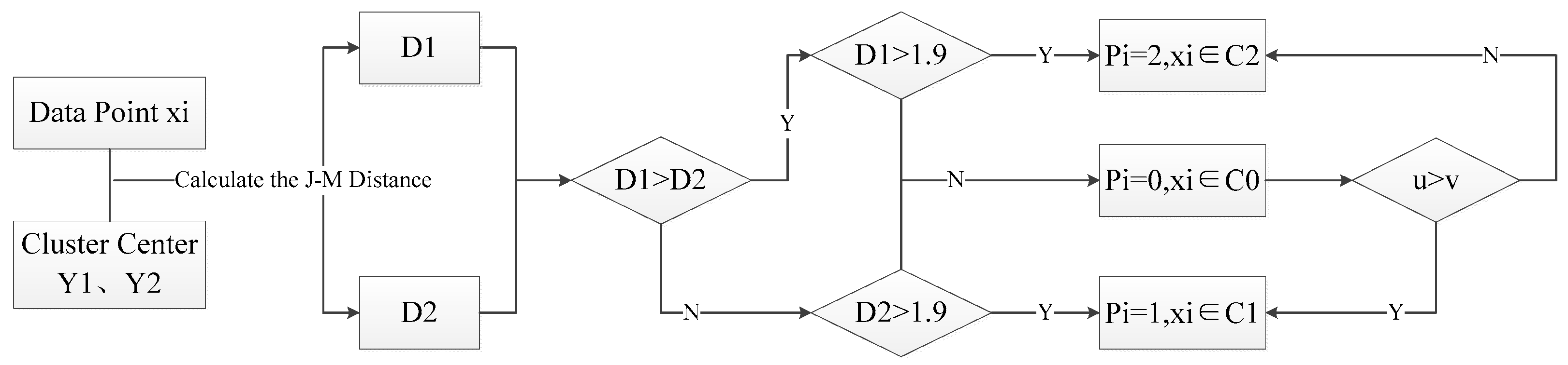
The targets studied in this paper only involve two categories, oil spills and seawater, so K = 2. For each set of data points in the image, calculate the J–M distances, and , to two cluster centers and , respectively, and use 1.9 as a measure to classify the center pixel: When and , , ; when and , , .
When the relationship between and does not belong to the above two cases, assume and and then judge according to the category of the eight pixels around the central pixel. Assuming that the number of points belonging to in the eight neighborhood pixels is u, and the number of points belonging to is v, if , then , ; if , then , . The classification process route is shown in Figure 3.
3.1.3. Iterations
After traversing the entire image, all pixels will be divided into two categories: and . Count the mean and standard deviation of each category as a new cluster center, and if the distance between the new cluster center and the previous group of cluster centers is less than a convergence threshold, the position of the recalculated cluster center has not changed much, the algorithm tends to be stable, and the clustering has reached the desired result. At this point, the algorithm can be terminated, and the segmented image is .
If the distance between the two groups of cluster centers has not yet reached the convergence threshold, step 2 needs to be repeated, and the pixel points are clustered again until the distance between the new cluster center and the previous group of cluster centers converges to set the threshold. In the experiment, the convergence threshold t = 0.05.
3.1.4. Integrated Filtering of Optimal Features
According to the results after segmentation, the mean and standard deviation of different categories on each feature are counted, and the corresponding J–M distance jm calculated. Then, the segmentation results are evaluated, and the 19 features are sorted according to the size of jm and the evaluation index as the preliminary screening results.
3.2. Data Acquisition and Processing
In 2014 and 2016, ESA, the European Commission, and the European Environment Agency implemented the Copernicus Project and launched Sentinel-1A and B under the Sentinel-1 series of satellites. The two satellites share an orbital plane with an orbital phase difference of 180. Sentinel-1A (S1A) is equipped with a C-band (5.405 GHz) SAR sensor with a standard revisit period of 12 days [33]. These data can be acquired in different acquisition modes, namely, SM (Stripmap mode), IW (interferometric wide swath mode), EW (extrawide swath mode) and WM (wave mode).
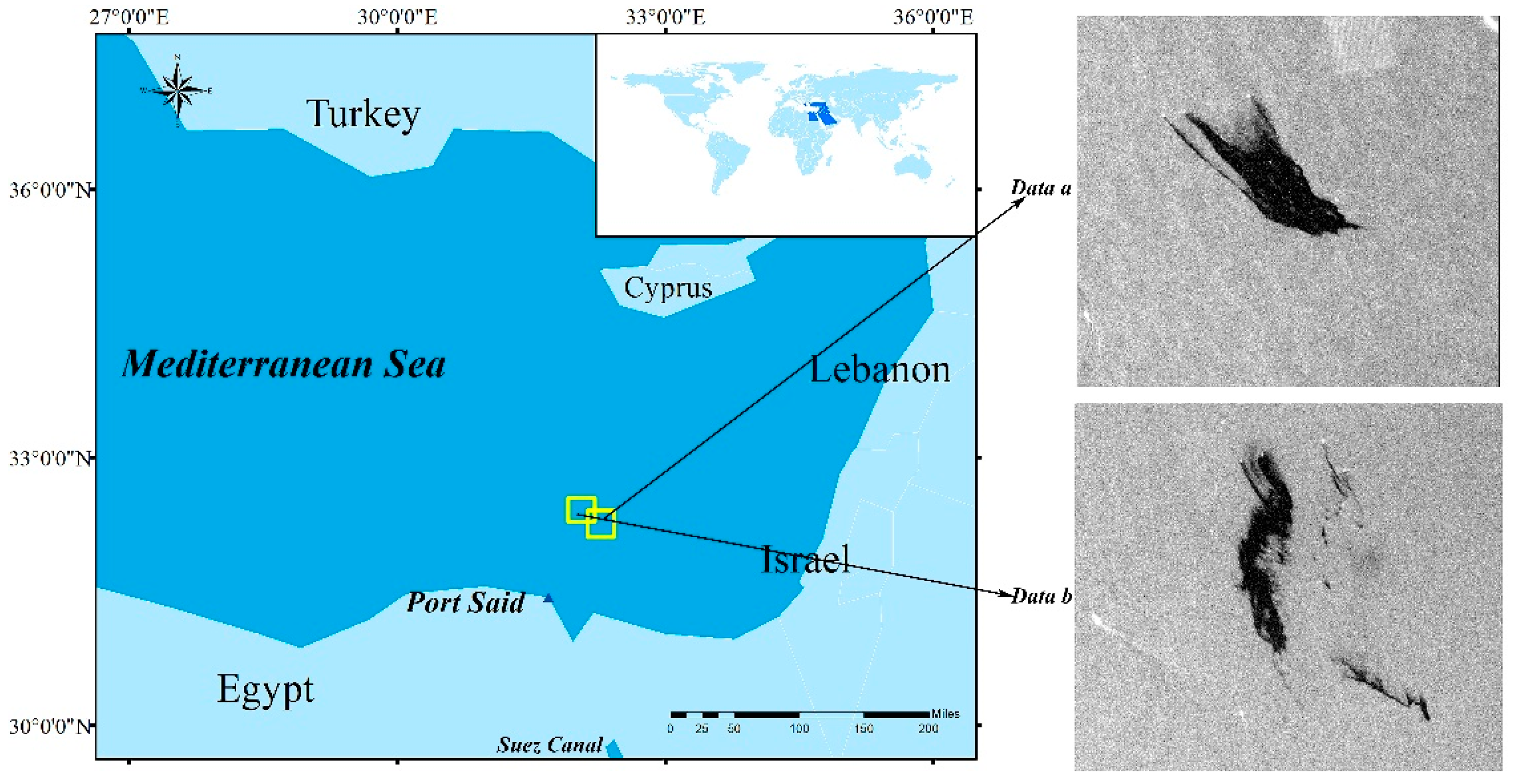
This paper takes the Suez Canal, which is an important international shipping canal connecting the Red Sea and the Mediterranean, as the research area. The northern entrance of the Suez Canal between longitude 32°7′13″E and 32°39′18″E, latitude 31°40′14″N, and 31°9′57″E was chosen as the source of oil spill data; S1A collected oil spill data a and b of the two scenes on 3 May 2017 and 20 July 2017. The data of both scenes are IW mode standard Level-1 SLC (Single Look Complex), and the polarized mode is VV + VH.
Figure 4 depicts the geographic area of the Suez Canal. The right side of Figure 4 shows the data of two scenes: a and b. The yellow boxes mark the specific positions of a and b in the vicinity of the port. To ensure that the final selected advantageous features had certain stability when applied to different images, we focused on the noise intensity of the two sets of data when acquiring the data. It can be seen from the figure that b has stronger speckle noise than a.
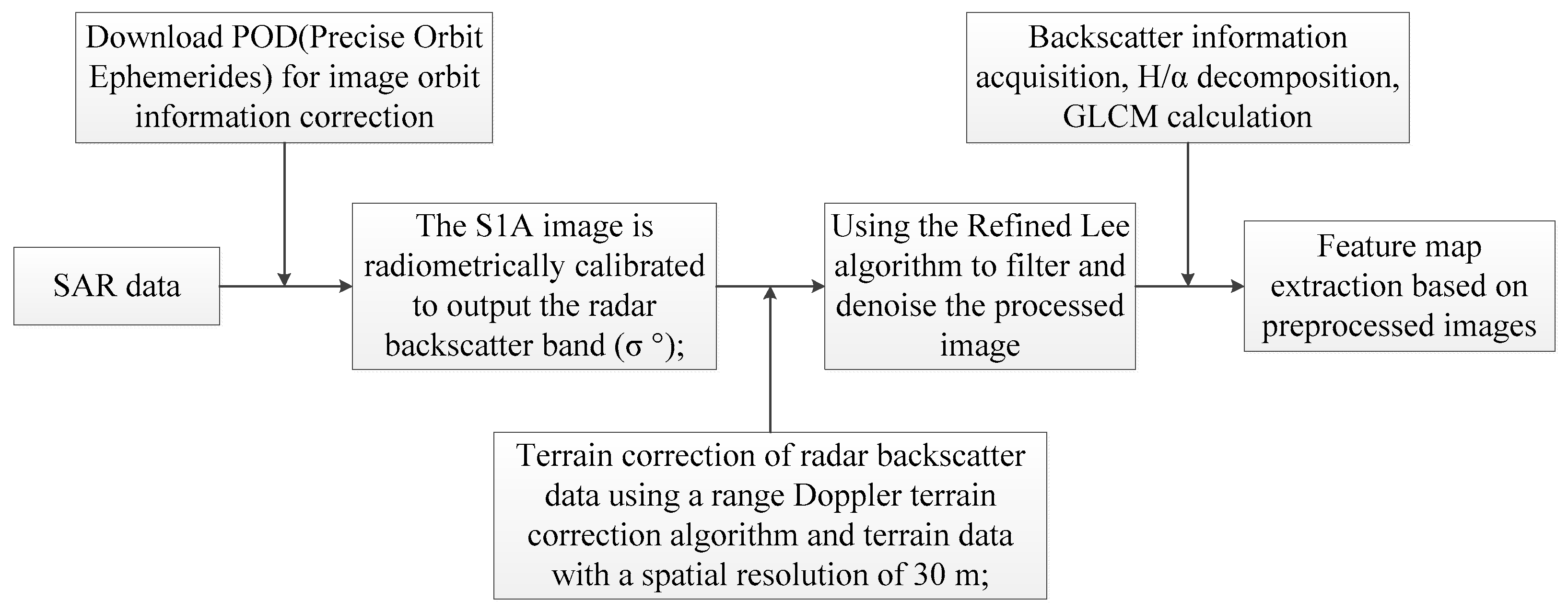
S1A data acquired at ESA need to be processed before they can be used for analysis. The specific steps of preprocessing include radiometric calibration, terrain correction, filtering, and denoising (Figure 5). Data preprocessing is based on the SNAP software platform (Sentinel Application Platform, http://step.esa.int/main/toolboxes/snap/, accessed on 11 October 2021) developed by ESA.
4. Results
4.1. Feature Extraction
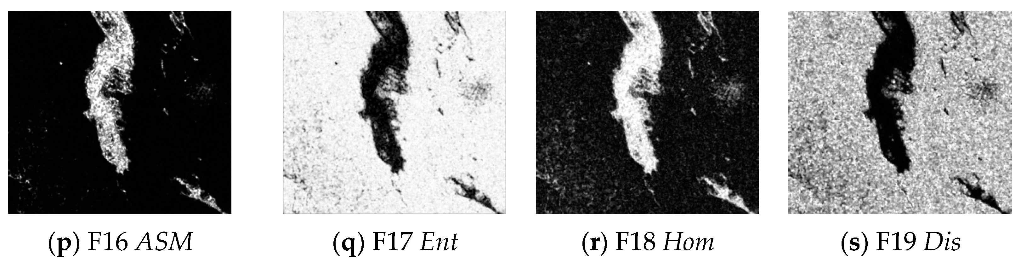
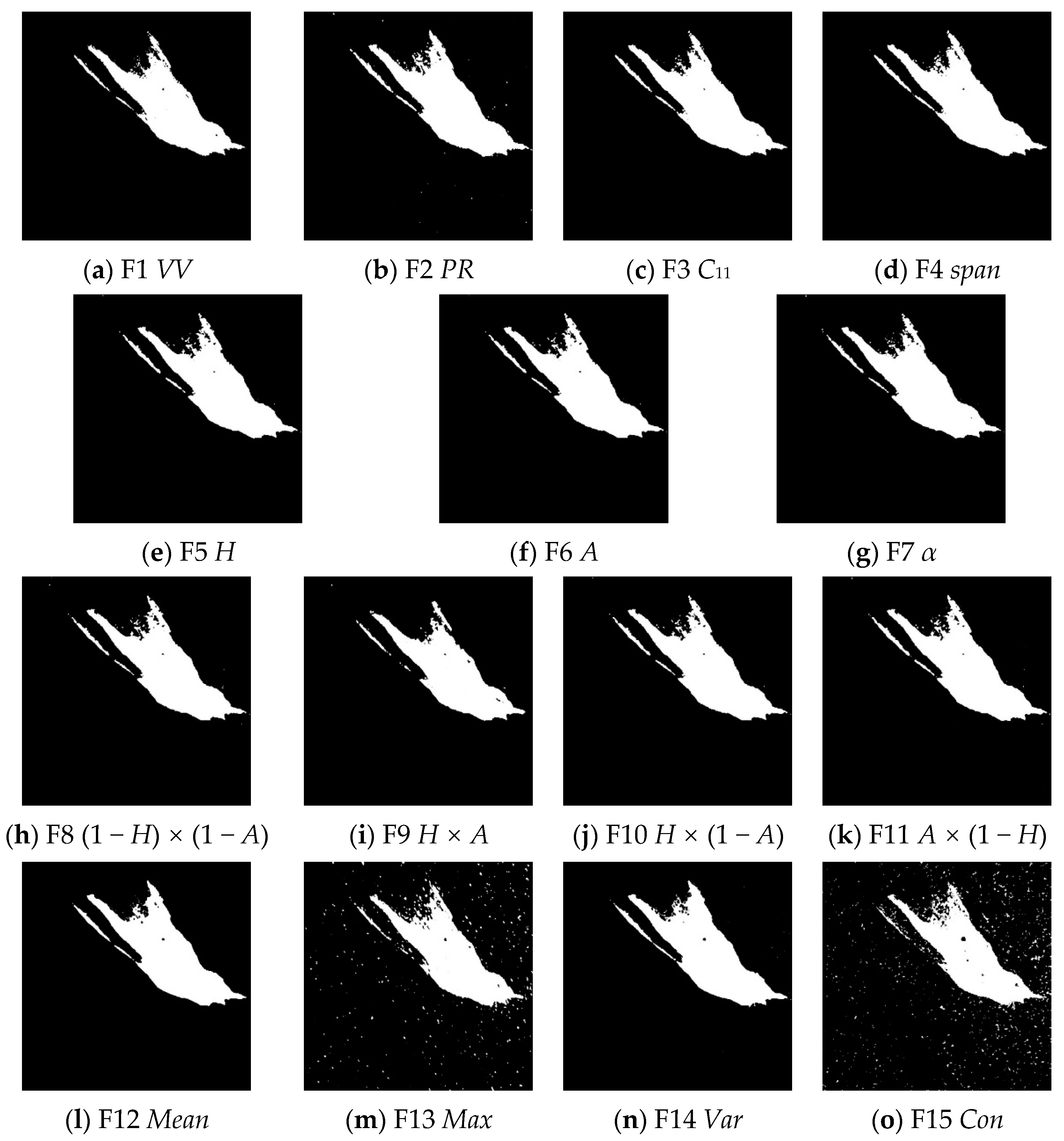
Feature extraction was performed on the preprocessed images of the two scenes, and the extracted features are shown in Figure 6 and Figure 7. The first row of the image shows the four features based on backscatter information, the second and third rows show the H-α polarimetric decomposition-based features and four combined features, namely , , and , and the last two rows show the eight features based on the grayscale co-occurrence matrix. It can be seen from the figure that the backscattering intensity VV and the four combined characteristic images based on H-α polarimetric decomposition are generally uniform in background, and there is a relatively clear boundary between the oil film and the seawater. The texture features based on the GLCMand other features, especially the images of F13, F14, and F15, have strong background noise. Noisier features may have negative effects for actual oil spill extraction.
4.2. Oil Spill Extraction Results
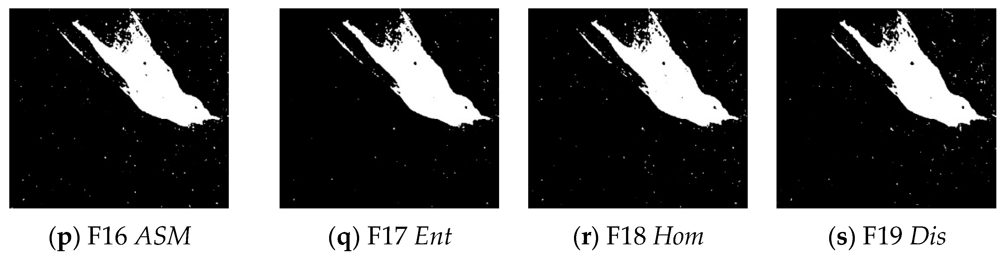
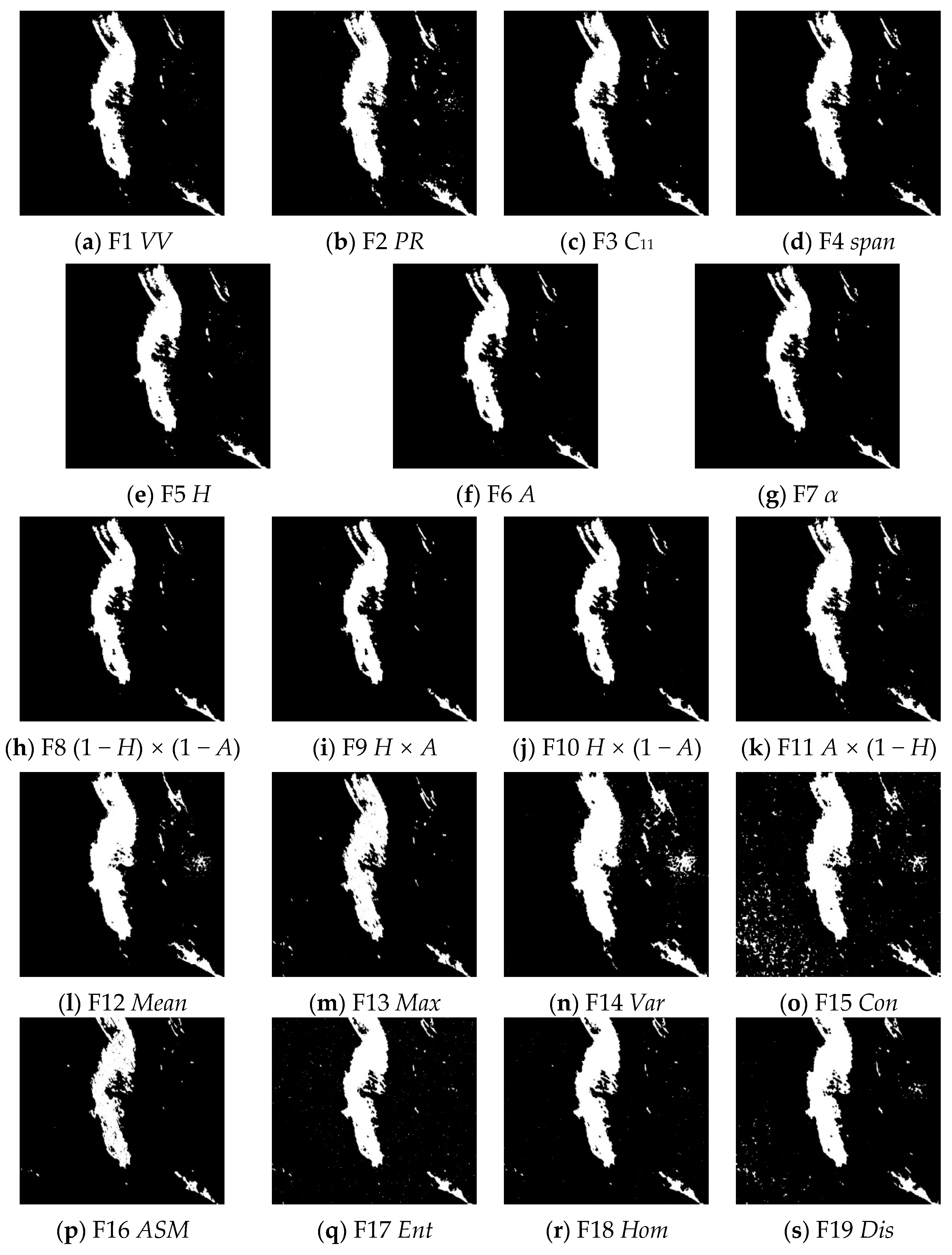
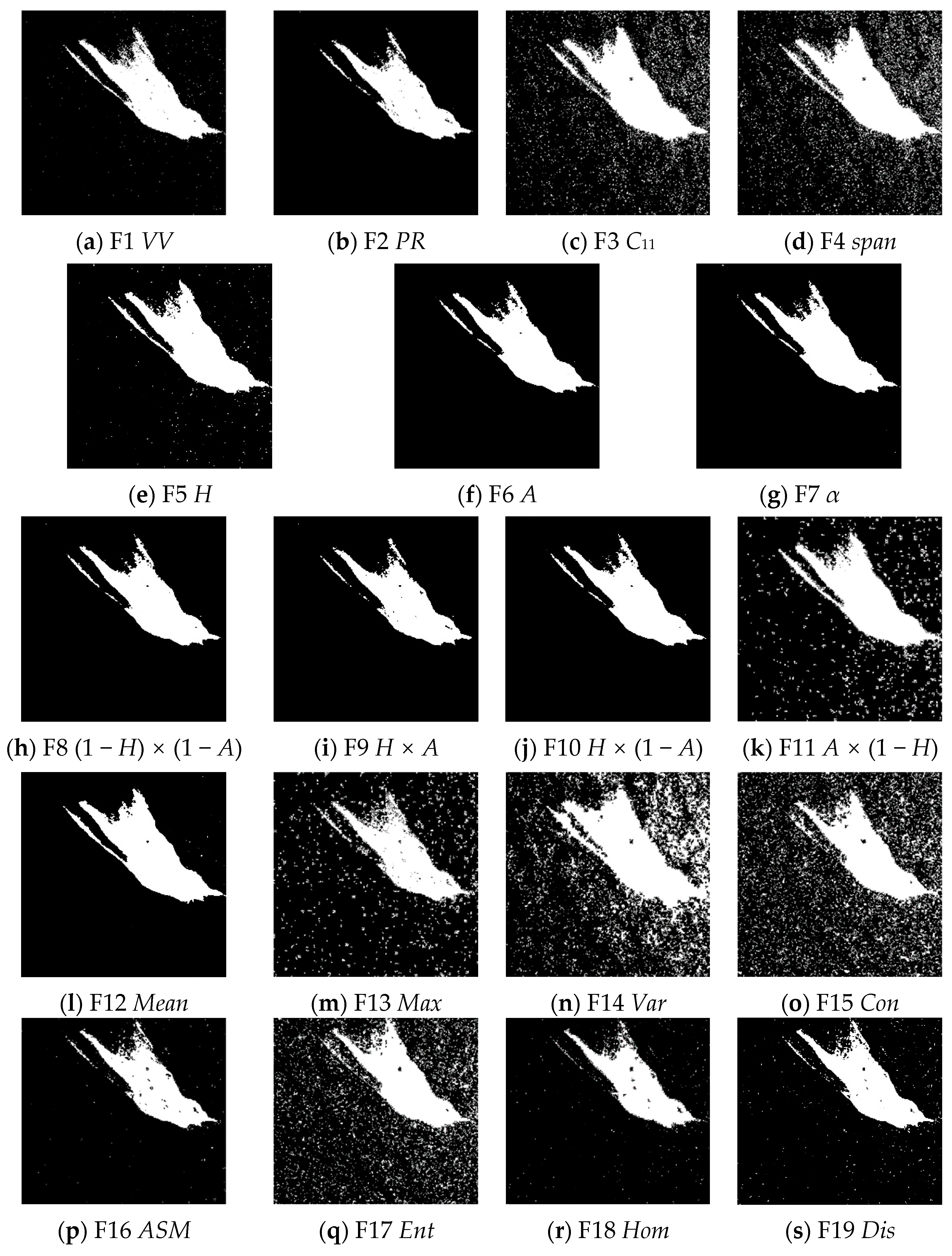
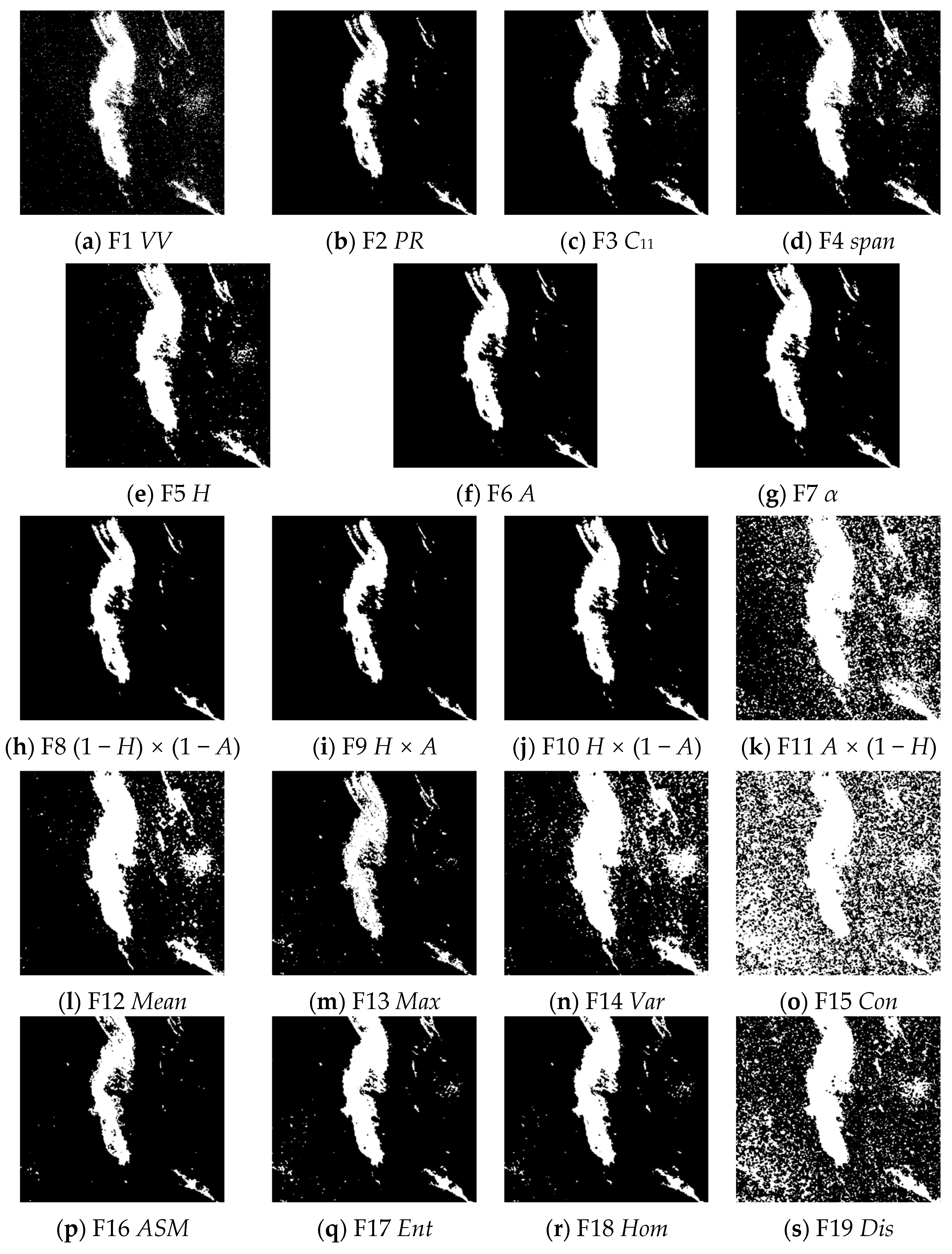
The improved J–M/K-means algorithm and K-means algorithm are used to segment the 19 feature maps of the data from the two scenes. Figure 8 and Figure 9 show the feature image segmentation results of a and b of the improved algorithm, respectively. Figure 10 and Figure 11 shows the segmentation results of the K-means algorithm.
Among these data images, the white part represents the area that is clustered as an oil spill, and the black part represents sea water. According to the segmentation results, it can be seen that the feature images with strong background noise such as F13, F14, and F15 still have strong background noise after segmentation, and the segmentation effect is poor. This phenomenon is more consistent with the above speculation, and actual feature screening will need to be conducted in further analysis.
4.3. Optimal Feature Evaluation
The advantage feature screening based on the improved J–M/K-means algorithm is divided into two stages. The first stage is the preliminary screening of dominant features: Calculate the J–M distance between oil spills and seawater on different feature images after segmentation and the overall accuracy OA of feature image segmentation and F1-score to obtain the preliminary screening results of dominant features.
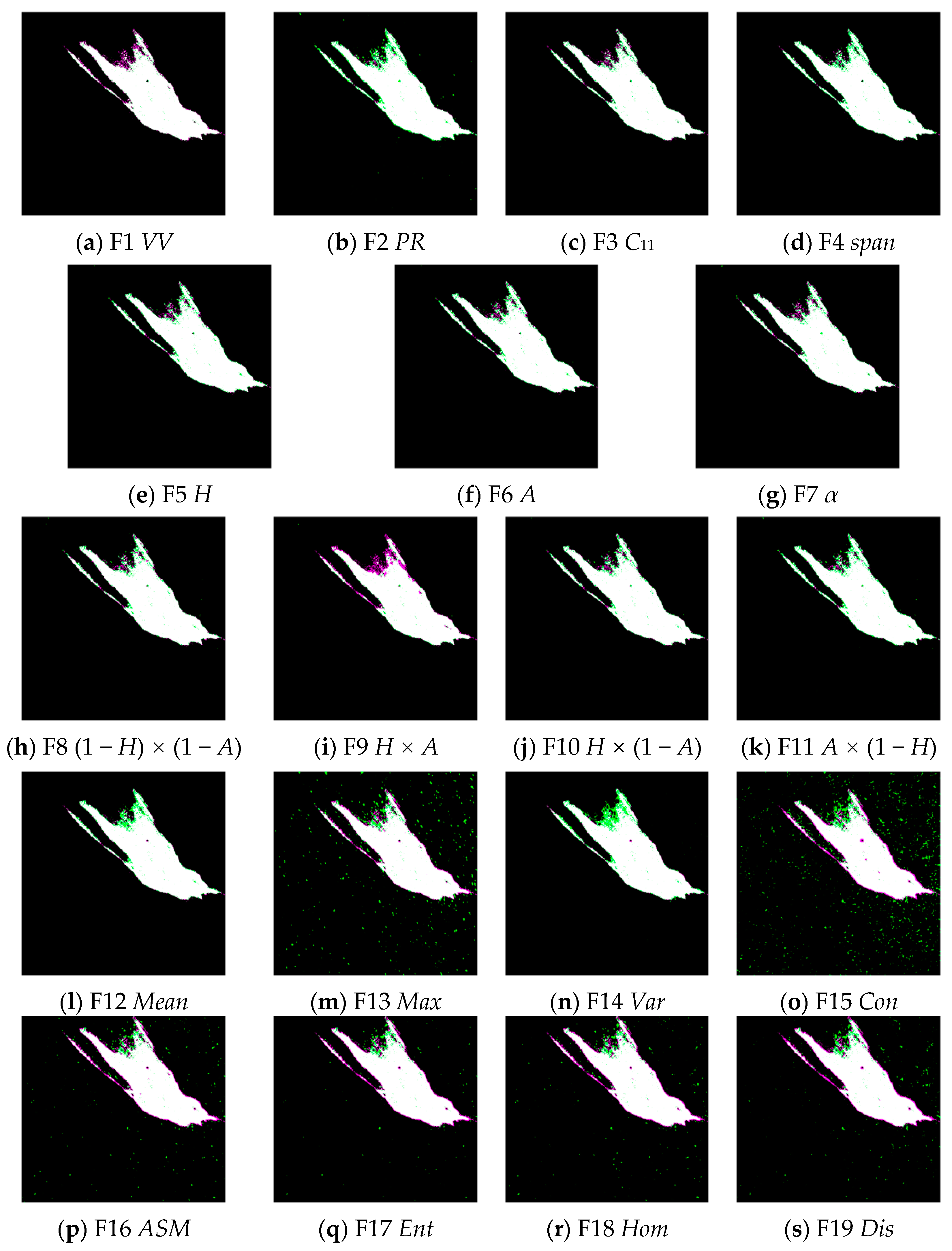
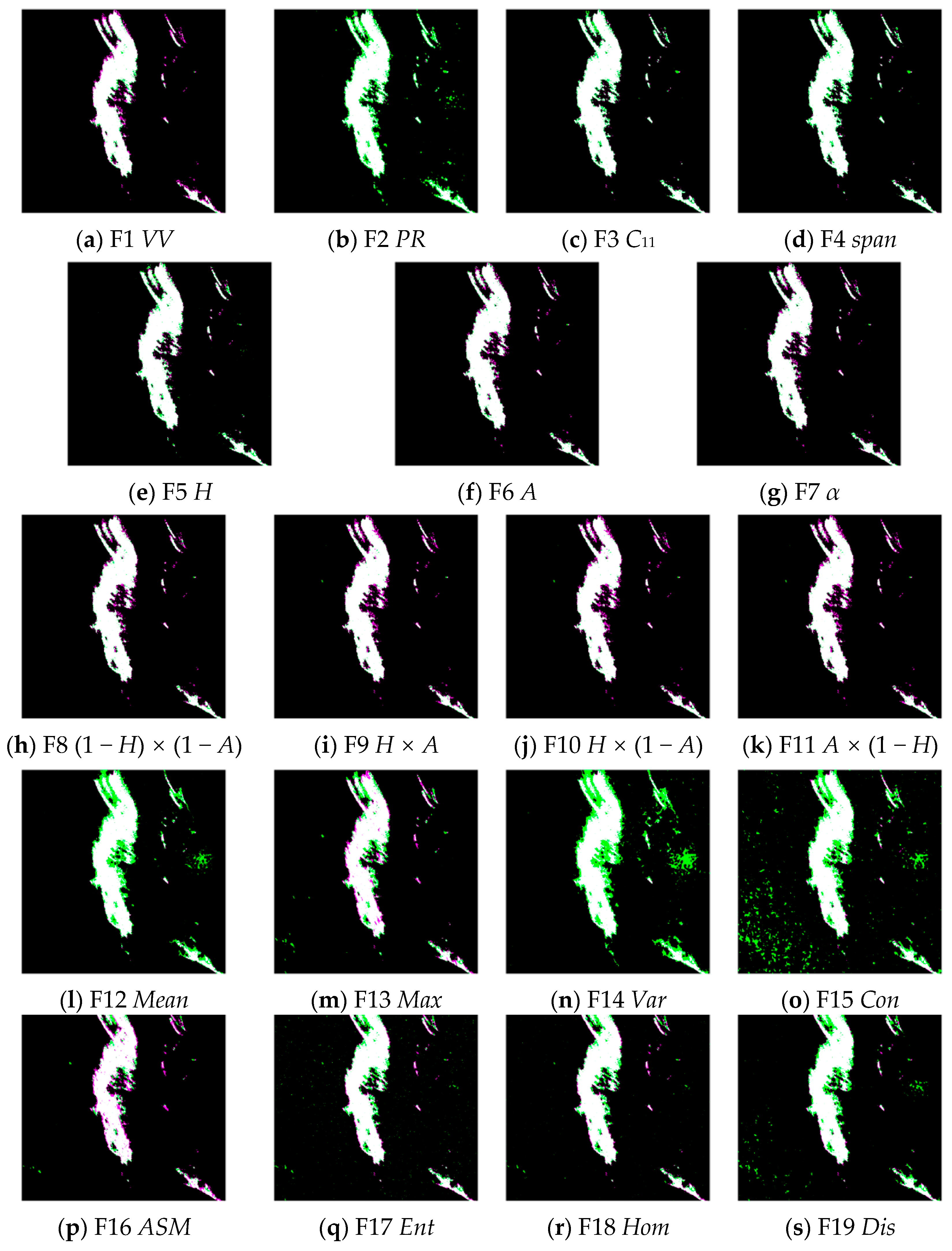
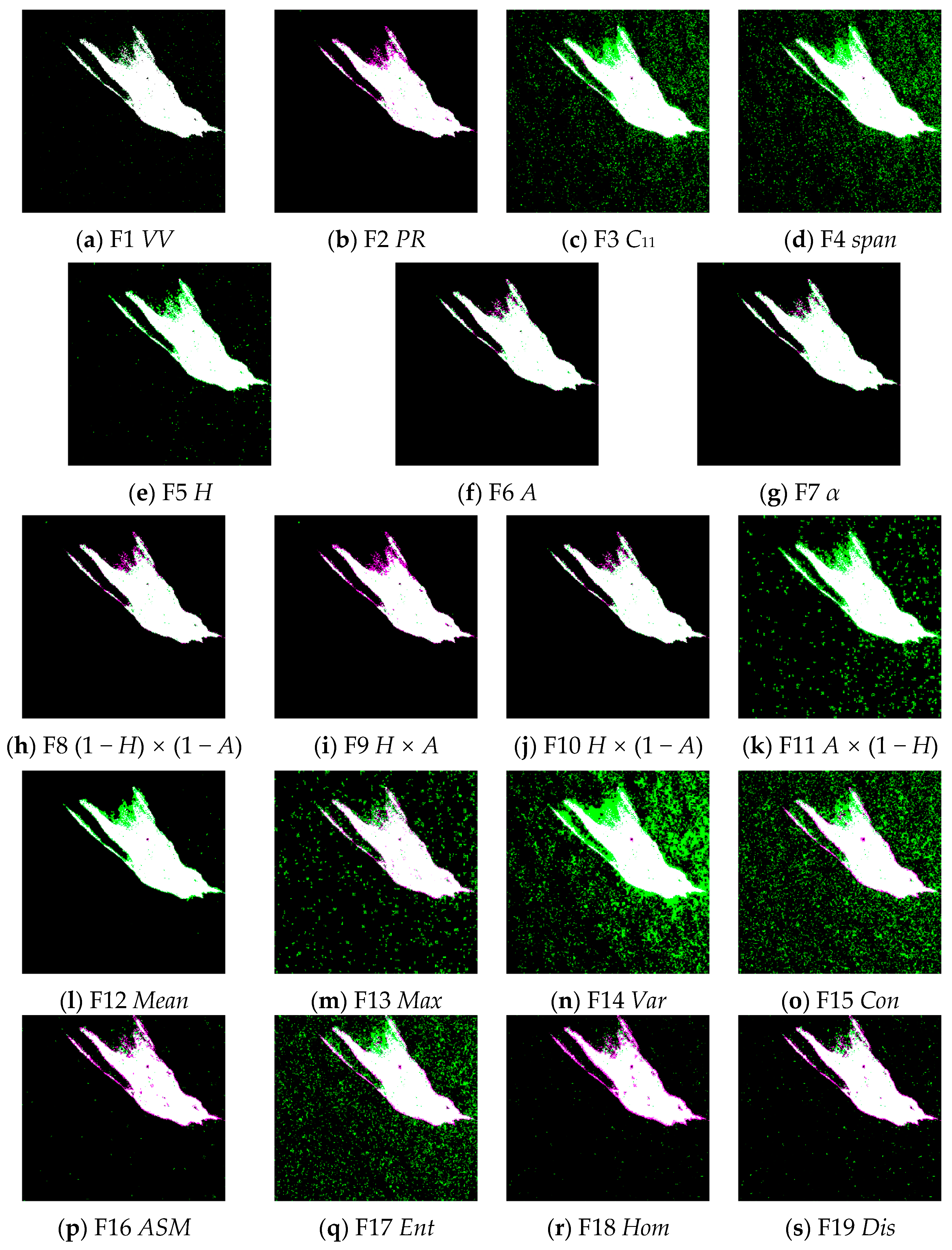
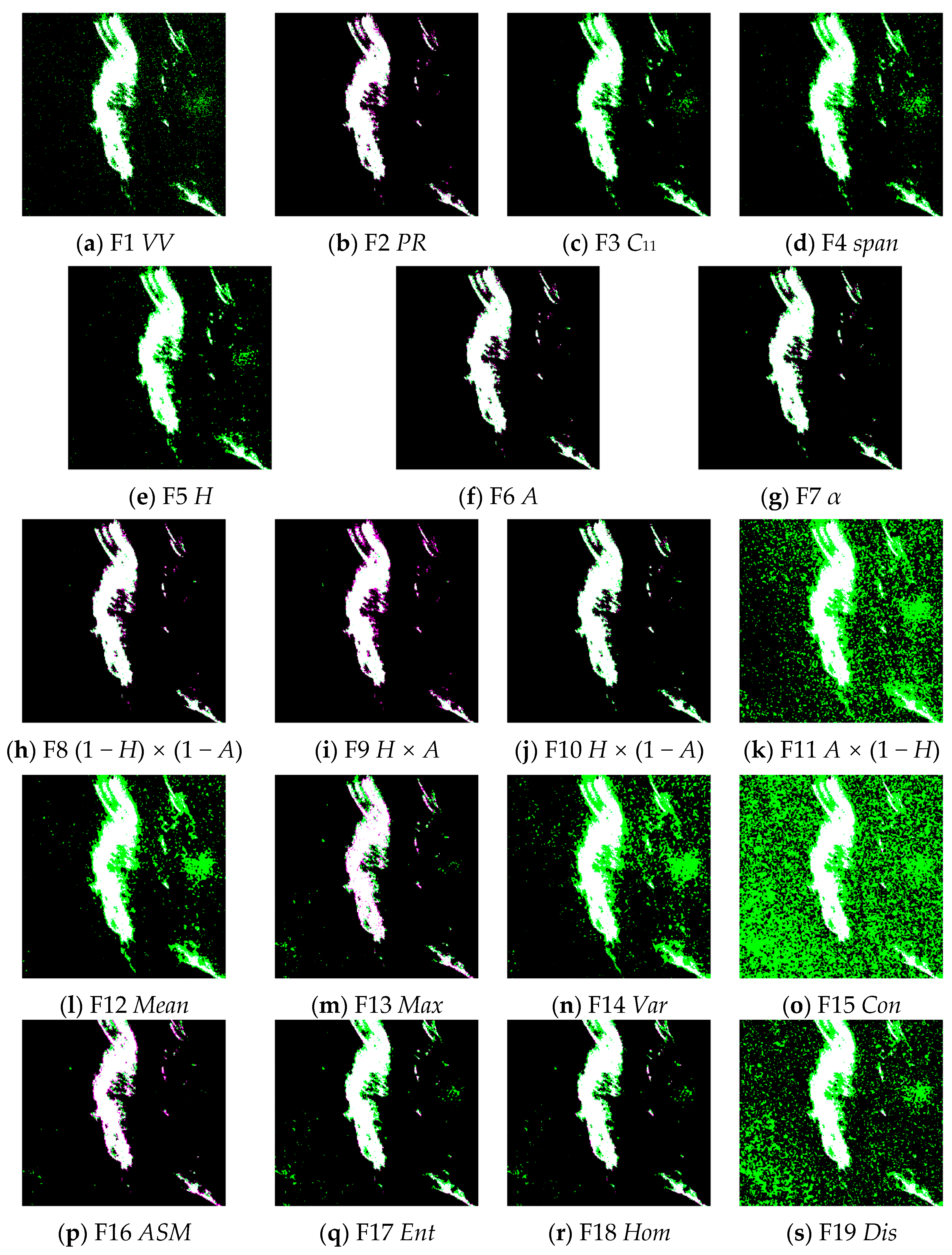
In the evaluation of image segmentation accuracy, the ground truth images are obtained based on expert interpretation and annotation [1]. After comparative evaluation, the image segmentation evaluation results for the two algorithms are shown in Figure 12, Figure 13, Figure 14 and Figure 15.
Figure 12, Figure 13, Figure 14 and Figure 15 show the evaluation results for each feature in the two sets of data. In the figure, the green part represents the pixels that are actually seawater and are classified as oil spills, and the red part represents the pixels that are actually oil spills and are classified as seawater.
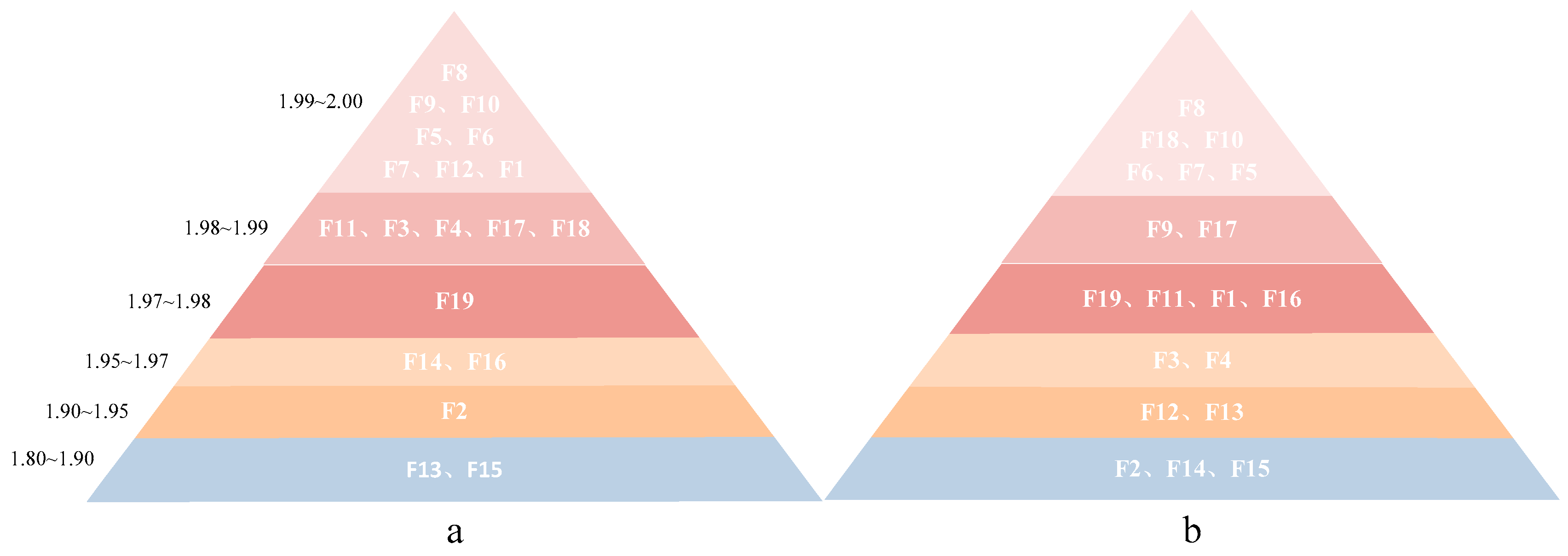
Calculate the J–M distance of each feature according to the segmentation result and divide all features into three gradients in order of distance from high to low. For the first gradient, the J–M distance is the largest, ranging from 1.97 to 2.00; for the second gradient, the J–M distance of the feature is between 1.90 and 1.97. When J–M < 1.90, it is considered that the feature falls into the third gradient, and the features falling within this range can distinguish samples but have a general effect. After determining the gradient of each feature, the dominant features are initially screened by comparing the overall accuracy of each feature in different gradients and the stability of their performance with the two sets of data. Table 2 and Table 3 and Figure 16, respectively, report the J–M distance and overall accuracy results for the 19 features of the two sets of data a and b, as well as the distribution of the 19 features on the three gradients.
5. Discussion
In the evaluation results for the two arithmetic methods in Section 4 of the analysis, it is possible to see that the K-means arithmetic method and the improved J–M/K-means arithmetic method are smooth. In addition, on the strong special strategy, the improved J–M/K-means algorithm’s split accuracy sum, F1, demonstrated clear superiority to the traditional K-means algorithm.
Moreover, Figure 16 shows that among the 19 features of data a, 14 features fall into the 1st gradient, 3 features fall into the 2nd gradient, and 2 features fall into the 3rd gradient. In the first gradient, except for F17, F18, and F19, the overall accuracy of the feature images is high, with F1 performing the best, and the overall accuracy OA is 98.7484%; F1 is 0.9473. In the second gradient, the F14 segmentation effect is the best, the overall accuracy reaches 97.8810%, and F1 is 0.9156. For data b, 12 features fall into the 1st gradient, 4 features fall into the 2nd gradient, and 3 features fall into the 3rd gradient. Since data b has stronger speckle noise than data a, the J–M distance and overall accuracy of these feature images are also relatively small. In the first gradient, except for F11, F17, F18, and F19, the overall accuracy of the feature images is greater than 97%, with F8 performing the best, and the overall accuracy OA is 98.0025%; F1 is 0.9038. In the second gradient, the F3 segmentation effect is the best, the overall accuracy reaches 97.4621%, and F1 is 0.8861. The samples are less separable on their images due to features falling within the third gradient and are not considered here.
The stability of multisource features under different noise images can be found from the feature distribution rules of the two groups of images a and b. It can be clearly seen from Figure 16 that among the 19 features of data a, 14 features are distributed in the first grad1stient, while only 12 features of data b fall into the 1st gradient. Additionally, the same features falling into the same gradient show better segmentation on data a. From this, it can be concluded that different images have different distributions of features, and their distribution results will be affected by the intensity of noise carried by different images. The smoother an image is, the more its features will fall into the first gradient, and the overall accuracy of the segmentation result will be higher; conversely, if an image has strong noise, the inter-class J–M distance will be affected by noise and outliers, the value will be relatively small, and the segmentation result will be worse. Therefore, in order to ensure that the selected features are advantageous for images with different noise levels, we selected the intersection of the two images in the first gradient and second gradient and selected the features whose overall accuracy was greater than 97% and F1 scores were higher than 0.8500 as the screening results of the first stage on the basis of the feature distribution shown in Figure 16.
The first-stage screening results contain a total of 11 features, namely F1, F3, F4, F5, F6, F7, F8, F9, F10, F16, and F18.
In the process of extracting SAR oil spill features, some features are derived from other features through transformation. For example, the four combined features of polarimetric decomposition are obtained by simple matrix operations on the basis of the three parameters of H-α decomposition. This situation will lead to the possibility that different features may carry a large amount of similar information. In order to avoid information redundancy, in the second stage, we divided the 11 features after preliminary screening into 3 categories according to the extraction basis and calculated the correlations between them; the features with the largest J–M distance and the groups of features with low correlations were reserved for the final screening results.
We selected the backscattering intensity VV, the polarimetric decomposition combination parameter , and the homogeneity Hom as the representative features of the three categories and calculated the correlations between the remaining 18 features and them respectively. From the calculation results of the correlation coefficients in Table 4, it can be seen that the features within the same category are highly correlated, and the information redundancy is greater, while the feature correlations between different categories are relatively low. Therefore, in the selection of dominant features, it is of great significance to consider combinations of features with different attributes to reduce information redundancy and the amount of calculation.
According to the analysis of the experimental results, when using dual-polarized SAR images for oil spill detection, the backscattering intensity VV, polarimetric decomposition combination parameters , and homogeneity Hom can be mainly considered. In addition, the polarimetric span, polarimetric entropy H, and second-order moment ASM can also be considered as subdominant features.
6. Conclusions
This paper focuses on the screening of multisource features in dual-polarized SAR oil spill detection. Considering the limitation that only using the J–M distance to filter the dominant features will be affected by the selection of training samples, we replace the Euclidean distance with the J–M distance and add the relationship between the neighborhood pixels and the center pixel in the process of data point generation to improve the traditional K-means algorithm, and we obtain a feature optimization algorithm based on J–M distance and overall accuracy. This method effectively avoids the interference of artificially selected samples on feature dominance and at the same time weakens the influence of noise. In addition, in order to reasonably reduce the amount of calculation and information redundancy, correlation analysis is carried out on the results of the feature preliminary screening based on the improved algorithm; finally, the backscattering intensity VV, the polarimetric decomposition combination parameter and the homogeneity Hom are determined. Three dominant features, polarimetric span, polarimetric entropy H, and the second-order moment ASM also performed well in the experiments and can be considered secondary dominant features in subsequent applications.
In order to ensure that the conclusions drawn in this article have strong applicability, the study selected two groups of data with different noise intensities for comparative experiments when acquiring data. Finally, the dominant and subdominant features were selected to have better performance with both groups of data. However, the performance of multisource features in dual-polarized SAR oil spill detection is also affected by satellite systems, imaging methods, bands, observation conditions, environmental conditions and other factors; therefore, the conclusions in this paper have high applicability to the Sentinel-1 oil spill datasets. To draw conclusions about the applicability of multisource features under different conditions, more images need to be collected for further research.
Author Contributions
Conceptualization, L.C.; methodology, L.C. and M.X.; software, L.C.; validation, L.C., M.X. and Y.L.; formal analysis, L.C. and X.Z.; writing—original draft preparation, L.C.; writing—review and editing, L.C. and M.X. All authors have read and agreed to the published version of the manuscript.
Funding
This research was funded in part by Liaoning Revitalization Talents Program, (grant number XLYC2001002) and in part by China National Key R&D Program (grant number 2020YFE0201500).
Data Availability Statement
The data that support the findings of this research are available at the corresponding author with reasonable request.
Acknowledgments
The authors would like to thank ESA for providing the Sentinel-1A data (https://scihub.copernicus.eu/, accessed on 11 October 2021).
Conflicts of Interest
The authors declare no conflict of interest.
References
- El-Magd, I.A.; Zakzouk, M.; Abdulaziz, A.M.; Ali, E.M. The potentiality of operational mapping of oil pollution in the mediterranean sea near the entrance of the suez canal using sentinel-1 SAR data. Remote Sens. 2020, 12, 1352. [Google Scholar] [CrossRef]
- Brekke, C.; Solberg, A.H.S. Oil spill detection by satellite remote sensing. Remote Sens. Environ. 2005, 95, 1–13. [Google Scholar] [CrossRef]
- Singha, S.; Bellerby, T.J.; Trieschmann, O. Detection and classification of oil spill and look-alike spots from SAR imagery using an Artificial Neural Network. In Proceedings of the 2012 IEEE International Geoscience and Remote Sensing Symposium, Munich, Germany, 22–27 July 2012. [Google Scholar] [CrossRef]
- Fingas, M. The Basics of Oil Spill Cleanup; CRC Press: Boca Raton, FL, USA, 2013. [Google Scholar] [CrossRef]
- Alpers, W.; Holt, B.; Zeng, K. Oil spill detection by imaging radars: Challenges and pitfalls. Remote Sens. Environ. 2017, 201, 133–147. [Google Scholar] [CrossRef]
- Fingas, M.; Brown, C. Review of oil spill remote sensing. Mar. Pollut. Bull. 2014, 83, 9–23. [Google Scholar] [CrossRef]
- Nunziata, F.; Gambardella, A.; Migliaccio, M. On the mueller scattering matrix for SAR sea oil slick observation. IEEE Geosci. Remote Sens. Lett. 2008, 5, 691–695. [Google Scholar] [CrossRef]
- Harris, A.H.S.; Chen, C.; Weisner, C.M.; Chalk, M.; Capoccia, V.; Thomas, C.P. Response to Dr Fiscella: Transparency and debate are essential to improve guidelines and measures. J. Addict. Med. 2016, 10, 453–454. [Google Scholar] [CrossRef]
- Topouzelis, K.; Stathakis, D.; Karathanassi, V. Investigation of genetic algorithms contribution to feature selection for oil spill detection. Int. J. Remote Sens. 2009, 30, 611–625. [Google Scholar] [CrossRef]
- Singha, S.; Velotto, D.; Lehner, S. Dual-polarimetric feature extraction and evaluation for oil spill detection: A near real time perspective. In Proceedings of the International Geoscience and Remote Sensing Symposium (IGARSS), Milan, Italy, 26–31 July 2015. [Google Scholar] [CrossRef]
- Mera, D.; Bolon-Canedo, V.; Cotos, J.; Alonso-Betanzos, A. On the use of feature selection to improve the detection of sea oil spills in SAR images. Comput. Geosci. 2017, 100, 166–178. [Google Scholar] [CrossRef]
- Niu, X.; Ban, Y.; Dou, Y. RADARSAT-2 fine-beam polarimetric and ultra-fine-beam SAR data for urban mapping: Comparison and synergy. Int. J. Remote Sens. 2015, 37, 2810–2830. [Google Scholar] [CrossRef]
- Skrunes, S.; Brekke, C.; Eltoft, T. Characterization of marine surface slicks by radarsat-2 multipolarization features. IEEE Trans. Geosci. Remote Sens. 2013, 52, 5302–5319. [Google Scholar] [CrossRef]
- Singha, S.; Ressel, R.; Velotto, D.; Lehner, S. A Combination of Traditional and Polarimetric Features for Oil Spill Detection Using TerraSAR-X. IEEE J. Sel. Top. Appl. Earth Obs. Remote Sens. 2016, 9, 4979–4990. [Google Scholar] [CrossRef]
- Yu, L.; Liu, H. Feature Selection for High-Dimensional Data: A Fast Correlation-Based Filter Solution. In Proceedings of the Twentieth International Conference on Machine Learning, Washington, DC, USA, 21–24 August 2003. [Google Scholar]
- Sulaiman, M.A.; Labadin, J. Feature selection based on mutual information. In Proceedings of the 2015 9th International Conference on IT in Asia (CITA), Sarawak, Malaysia, 4–5 August 2015. [Google Scholar] [CrossRef]
- Ma, X.; Xu, J.; Wu, P.; Kong, P. Oil Spill Detection Based on Deep Convolutional Neural Networks Using Polarimetric Scattering Information from Sentinel-1 SAR Images. IEEE Trans. Geosci. Remote Sens. 2021, 60, 1–13. [Google Scholar] [CrossRef]
- Prastyani, R.; Basith, A. Utilisation of Sentinel-1 SAR Imagery for Oil Spill Mapping: A Case Study of Balikpapan Bay Oil Spill. JGISE J. Geospat. Inf. Sci. Eng. 2018, 1, 22–26. [Google Scholar] [CrossRef]
- Kim, D.; Jung, H.S. Mapping oil spills from dual-polarized sar images using an artificial neural network: Application to oil spill in the kerch strait in november 2007. Sensors 2018, 18, 2237. [Google Scholar] [CrossRef] [PubMed]
- Li, H.; Perrie, W.; He, Y.; Wu, J.; Luo, X. Analysis of the Polarimetric SAR Scattering Properties of Oil-Covered Waters. IEEE J. Sel. Top. Appl. Earth Obs. Remote Sens. 2014, 8, 3751–3759. [Google Scholar] [CrossRef]
- Chaturvedi, S.K.; Banerjee, S.; Lele, S. An assessment of oil spill detection using Sentinel 1 SAR-C images. J. Ocean Eng. Sci. 2019, 5, 116–135. [Google Scholar] [CrossRef]
- Alpers, W.; Hühnerfuss, H. The damping of ocean waves by surface films: A new look at an old problem. J. Geophys. Res. 1989, 94, 6251–6265. [Google Scholar] [CrossRef]
- Cloude, S.R.; Pottier, E. An entropy based classification scheme for land applications of polarimetric SAR. IEEE Trans. Geosci. Remote Sens. 1997, 35, 68–78. [Google Scholar] [CrossRef]
- Schuler, D.L.; Lee, J.S. Mapping ocean surface features using biogenic slick-fields and SAR polarimetric decomposition techniques. IEE Proc. Radar Sonar Navig. 2006, 153, 260–270. [Google Scholar] [CrossRef]
- Mubea, K.; Menz, G. Monitoring Land-Use Change in Nakuru (Kenya) Using Multi-Sensor Satellite Data. Adv. Remote Sens. 2012, 1, 74–84. [Google Scholar] [CrossRef]
- Shi, N.; Liu, X.; Guan, Y. Research on k-means clustering algorithm: An improved k-means clustering algorithm. In Proceedings of the 2010 Third International Symposium on Intelligent Information Technology and Security Informatics, Jian, China, 2–4 April 2010. [Google Scholar] [CrossRef]
- Sun, J.G.; Liu, J.; Zhao, L.Y. Clustering algorithms research. J. Softw. 2008, 19, 48–61. [Google Scholar] [CrossRef]
- Fahim, A.M.; Salem, A.M.; Torkey, F.A.; Ramadan, M.A. Efficient enhanced k-means clustering algorithm. J. Zhejiang Univ. Sci. 2006, 7, 1626–1633. [Google Scholar] [CrossRef]
- Bruzzone, L.; Roli, F.; Serpico, S.B. An Extension of the Jeffreys-Matusita Distance to Multiclass Cases for Feature Selection. IEEE Trans. Geosci. Remote Sens. 1995, 33, 1318–1321. [Google Scholar] [CrossRef]
- Dabboor, M.; Howell, S.; Shokr, M.; Yackel, J. The Jeffries–Matusita distance for the case of complex Wishart distribution as a separability criterion for fully polarimetric SAR data. Int. J. Remote Sens. 2014, 35, 6859–6872. [Google Scholar] [CrossRef]
- Klein, D.; Moll, A.; Menz, G. Land cover/land use classification in a semiarid environment in East Africa using multi-temporal alternating polarisation ENVISAT ASAR data. In Proceedings of the 2004 Envisat & ERS Symposium (ESA SP-572), Salzburg, Austria, 6–10 September 2004. [Google Scholar]
- Duda, R.O.; Hart, P.E.; Stork, D.G. Pattern Classification and Scene Analysis; Wiley: New York, NY, USA, 2001; Volume 10. [Google Scholar]
- Torres, R.; Snoeij, P.; Geudtner, D.; Bibby, D.; Davidson, M.; Attema, E.; Potin, P.; Rommen, B.; Floury, N.; Brown, M.; et al. GMES Sentinel-1 mission. Remote Sens. Environ. 2012, 120, 9–24. [Google Scholar] [CrossRef]
Figure 1.
Workflow of weakly supervised model for oil emulsion detection and identification.

Figure 2.
Data point generation. The left is the original image, the right is the expanded image, and the red box marks the selection method of data points.
Figure 2.
Data point generation. The left is the original image, the right is the expanded image, and the red box marks the selection method of data points.

Figure 3.
Workflow of the classification process.

Figure 4.
Study area.

Figure 5.
Data preprocessing process.

Figure 6.
Data a Oil Spill Detection Features.


Figure 7.
Data b Oil Spill Detection Features.


Figure 8.
Image segmentation result for data a based on J–M/K-means algorithm.


Figure 9.
Image segmentation result for data b based on J–M/K-means algorithm.

Figure 10.
Image segmentation result for data a based on K-means algorithm.

Figure 11.
Image segmentation result for data b based on K-means algorithm.

Figure 12.
Evaluation results for data a based on J–M/K-means algorithm.

Figure 13.
Evaluation results for data b based on J–M/K-means algorithm.

Figure 14.
Evaluation results for data a based on K-means algorithm.

Figure 15.
Evaluation results for data b based on K-means algorithm.

Figure 16.
Feature gradient distribution map of data a and data b: red for the first gradient, orange for the second gradient, blue for the third gradient. The depth of the color represents a numerical change in the J–M distance. The lighter the color, the larger the J–M distance of the corresponding feature, and the better the separability of oil spill and seawater.


Table 1.
Oil Spill Detection Feature Parameter.
| No. | Feature Parameters | No. | Feature Parameters |
|---|---|---|---|
| F1 | VV | F11 | |
| F2 | PR | F12 | Mean |
| F3 | F13 | Max | |
| F4 | span | F14 | Var |
| F5 | H | F15 | Con |
| F6 | A | F16 | ASM |
| F7 | α | F17 | Ent |
| F8 | F18 | Hom | |
| F9 | F19 | Dis | |
| F10 |
Table 2.
Oil spill detection feature J–M distance and evaluation results of data a.
| Features | Data a | ||||
|---|---|---|---|---|---|
| J–M Distance | J–M/K-Means | K-Means | |||
| OA (%) | F1-Score | OA (%) | F1-Score | ||
| F1 | 1.9921 | 98.7484 | 0.9473 | 98.3521 | 0.9727 |
| F2 | 1.9458 | 97.8102 | 0.9131 | 96.9753 | 0.9459 |
| F3 | 1.9881 | 98.5437 | 0.9400 | 90.6547 | 0.7100 |
| F4 | 1.9873 | 98.3641 | 0.9335 | 88.4134 | 0.6643 |
| F5 | 1.9978 | 98.3938 | 0.9342 | 95.7515 | 0.8448 |
| F6 | 1.9977 | 98.4757 | 0.9372 | 98.2294 | 0.9391 |
| F7 | 1.9967 | 98.4797 | 0.9373 | 98.3945 | 0.9342 |
| F8 | 1.9991 | 98.4354 | 0.9357 | 98.3945 | 0.9342 |
| F9 | 1.9980 | 98.5409 | 0.9373 | 98.3544 | 0.9386 |
| F10 | 1.9980 | 98.4439 | 0.9361 | 98.5897 | 0.9412 |
| F11 | 1.9888 | 98.1813 | 0.9265 | 93.3088 | 0.7757 |
| F12 | 1.9945 | 98.3279 | 0.9321 | 97.1466 | 0.8902 |
| F13 | 1.8528 | 95.0325 | 0.8175 | 94.4387 | 0.7939 |
| F14 | 1.9556 | 97.881 | 0.9156 | 80.0580 | 0.5361 |
| F15 | 1.8622 | 91.5522 | 0.7221 | 84.8239 | 0.5816 |
| F16 | 1.9547 | 96.888 | 0.8760 | 96.0729 | 0.9130 |
| F17 | 1.9866 | 97.7798 | 0.9082 | 88.7230 | 0.6580 |
| F18 | 1.9833 | 97.1032 | 0.9031 | 97.5047 | 0.8855 |
| F19 | 1.9778 | 96.5964 | 0.8650 | 94.9984 | 0.8131 |
Table 3.
Oil spill detection feature J–M distance and evaluation results of data b.
| Features | Data b | ||||
|---|---|---|---|---|---|
| J–M Distance | J–M/K-Means | K-Means | |||
| OA (%) | F1-Score | OA (%) | F1-Score | ||
| F1 | 1.9747 | 97.9358 | 0.9002 | 94.6913 | 0.8912 |
| F2 | 1.8959 | 95.3243 | 0.8105 | 93.4798 | 0.9220 |
| F3 | 1.9639 | 97.4621 | 0.8861 | 98.2877 | 0.8440 |
| F4 | 1.965 | 97.3563 | 0.8821 | 94.1398 | 0.7743 |
| F5 | 1.9927 | 97.3739 | 0.8812 | 95.3569 | 0.8122 |
| F6 | 1.9963 | 97.9493 | 0.9025 | 96.6453 | 0.9334 |
| F7 | 1.9955 | 97.8863 | 0.8998 | 98.3303 | 0.9213 |
| F8 | 1.9987 | 98.0025 | 0.9038 | 97.6323 | 0.9310 |
| F9 | 1.9855 | 97.9671 | 0.9003 | 98.0781 | 0.9085 |
| F10 | 1.9973 | 97.9644 | 0.9029 | 97.4353 | 0.9257 |
| F11 | 1.9763 | 95.2649 | 0.8562 | 73.0269 | 0.4272 |
| F12 | 1.9305 | 94.741 | 0.7916 | 89.4161 | 0.6552 |
| F13 | 1.9214 | 96.7051 | 0.8503 | 97.0304 | 0.8575 |
| F14 | 1.8726 | 91.966 | 0.7141 | 84.4316 | 0.5637 |
| F15 | 1.8327 | 89.9984 | 0.6641 | 48.7413 | 0.2810 |
| F16 | 1.9744 | 97.2142 | 0.8666 | 97.1910 | 0.8784 |
| F17 | 1.9808 | 93.8082 | 0.7570 | 94.8436 | 0.8618 |
| F18 | 1.9981 | 96.2694 | 0.8780 | 96.0215 | 08680 |
| F19 | 1.9774 | 95.2649 | 0.8056 | 80.6899 | 0.5090 |
Table 4.
Calculation results for the correlation between the dominant features of dual-polarized SAR oil spill.
Table 4.
Calculation results for the correlation between the dominant features of dual-polarized SAR oil spill.
| Category | No. | Feature | J–M Distance | Correlation Coefficient | ||
|---|---|---|---|---|---|---|
| with VV | with | with Hom | ||||
| Features based on backscatter information | F1 | VV | 1.9834 | 1 | 0.8830 | −0.7925 |
| F4 | span | 1.9761 | 0.8998 | 0.8242 | −0.7512 | |
| F3 | 1.9760 | 0.9033 | 0.8283 | −0.7506 | ||
| Features based on H-α polarimetric decomposition | F8 | 1.9989 | 0.8830 | 1 | −0.8548 | |
| F10 | 1.9977 | −0.9114 | −0.9788 | 0.8470 | ||
| F6 | A | 1.9970 | 0.9123 | 0.9719 | −0.8404 | |
| F7 | α | 1.9961 | −0.9121 | −0.9634 | 0.8353 | |
| F5 | H | 1.9953 | −0.8958 | −0.9026 | 0.7991 | |
| F9 | 1.9917 | 0.8405 | 0.9852 | −0.8221 | ||
| Features based on gray level co-occurrence matrix | F18 | Hom | 1.9907 | −0.7925 | −0.8548 | 1 |
| F16 | ASM | 1.9645 | −0.8271 | −0.9113 | 0.9303 | |
Publisher’s Note: MDPI stays neutral with regard to jurisdictional claims in published maps and institutional affiliations. |
© 2022 by the authors. Licensee MDPI, Basel, Switzerland. This article is an open access article distributed under the terms and conditions of the Creative Commons Attribution (CC BY) license (https://creativecommons.org/licenses/by/4.0/).
Share and Cite
MDPI and ACS Style
Cheng, L.; Li, Y.; Zhang, X.; Xie, M. An Analysis of the Optimal Features for Sentinel-1 Oil Spill Datasets Based on an Improved J–M/K-Means Algorithm. Remote Sens. 2022, 14, 4290. https://0-doi-org.brum.beds.ac.uk/10.3390/rs14174290
AMA Style
Cheng L, Li Y, Zhang X, Xie M. An Analysis of the Optimal Features for Sentinel-1 Oil Spill Datasets Based on an Improved J–M/K-Means Algorithm. Remote Sensing. 2022; 14(17):4290. https://0-doi-org.brum.beds.ac.uk/10.3390/rs14174290
Chicago/Turabian StyleCheng, Lingxiao, Ying Li, Xiaohui Zhang, and Ming Xie. 2022. "An Analysis of the Optimal Features for Sentinel-1 Oil Spill Datasets Based on an Improved J–M/K-Means Algorithm" Remote Sensing 14, no. 17: 4290. https://0-doi-org.brum.beds.ac.uk/10.3390/rs14174290
Note that from the first issue of 2016, this journal uses article numbers instead of page numbers. See further details here.