

Detailed Processes of Tidal Flat Geomorphology Evolution Based on Time-Series Satellite Images


1
Department of Geography and Spatial Information Techniques, Ningbo University, Ningbo 315211, China
2
Institute of East China Sea, Ningbo University, Ningbo 315211, China
3
Chongqing Institute of Meteorological Sciences, Chongqing 401147, China
4
State Key Laboratory of Estuarine and Coastal Research, East China Normal University, Shanghai 200062, China
5
School of Resources and Environment, Chengdu University of Information Technology, Chengdu 610225, China
*
Author to whom correspondence should be addressed.
Remote Sens. 2022, 14(17), 4341; https://0-doi-org.brum.beds.ac.uk/10.3390/rs14174341
Submission received: 22 June 2022
/
Revised: 28 August 2022
/
Accepted: 30 August 2022
/
Published: 1 September 2022
(This article belongs to the Special Issue Remote Sensing Application in Coastal Geomorphology and Processes)
Abstract
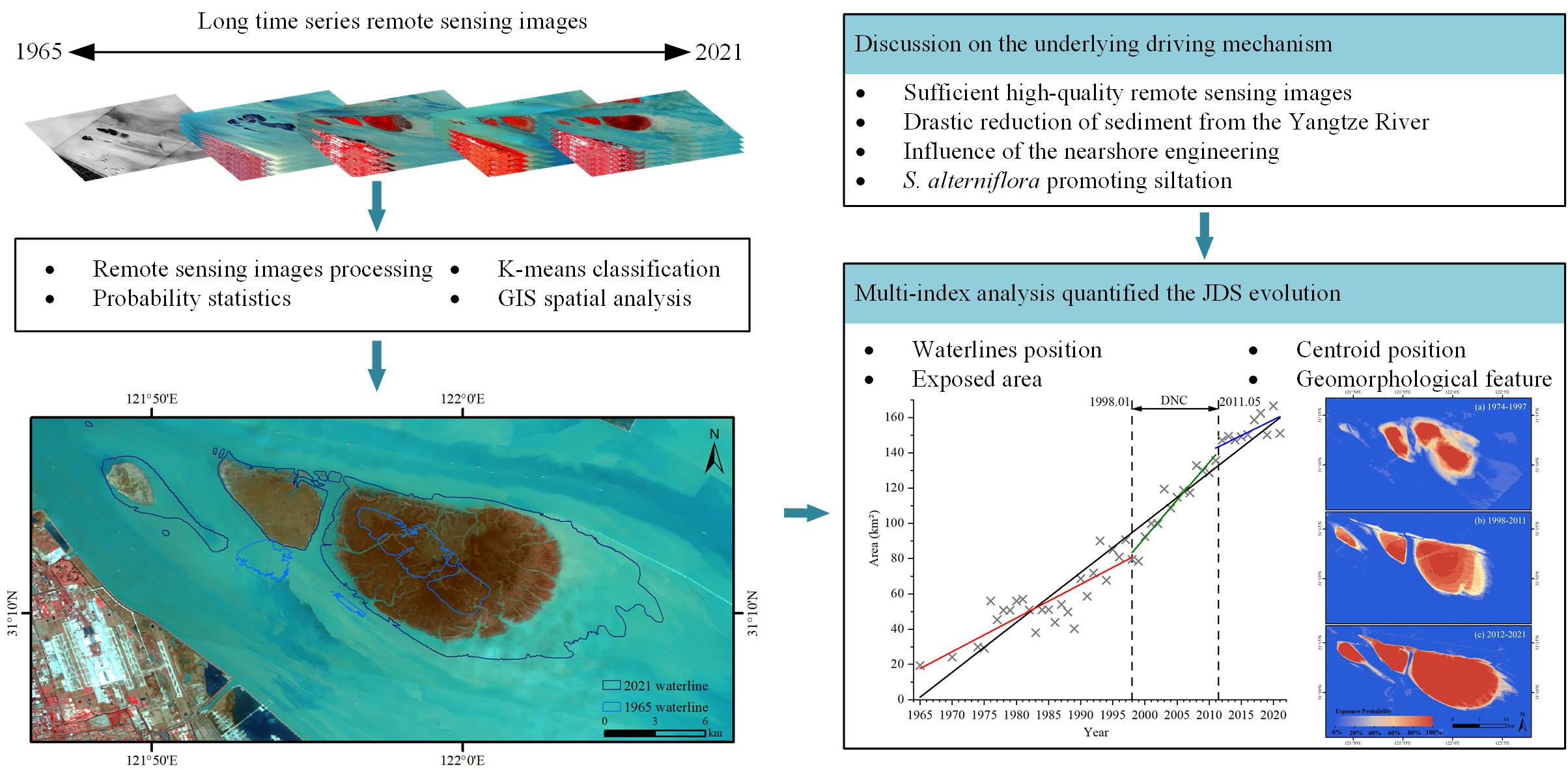
:In-depth understanding of long-term evolution of mega deltas with a large population is of great significance for national sustainability development programs. However, due to insufficient satellite images and its low temporal resolution, previous studies have only roughly explored the long-term evolution. To reveal the detailed delta evolution processes, Jiuduansha (JDS) upon the Yangtze estuary, which is one of the world’s mega deltas, was taken as an example. Based on the continuous time series of 792 satellite images between 1965 and 2021, this study combined the K-means classification, probability statistics, and GIS spatial analysis to generate the annual probability waterlines. Furthermore, the continuous time series of geomorphological features, position of waterlines and centroid change were determined. The results showed that the JDS exposed area presented a rapid growth trend. Specifically, in the early period (1965–1998), it presented a natural evolution state of “the head erosion, the tail deposition, and extending to the southeast”. In the recent period (1999–2021), the evolution state changed into the engineering-dominated evolution state of “erosion in the south, deposition in the north, continuous extension to the southeast, and overall northward movement”. The accelerated deposition of JDS over the recent 20 years has been mainly attributed to human activities, including the construction of Deep-water Navigation Channels and the vegetation promoting silting, followed by the upstream and downstream sediment sources. Current results suggest the JDS is likely to be more elongated in the SE-NW direction, with erosion in the southern region.

1. Introduction
Under the effects of the current global warming [1], sea level rising [2], drastic riverine sediment reduction [3], and high-intensity human activities (such as estuarine enclosures, damming in the middle and upper reaches of rivers, and construction of deep-water channels in estuaries) [4,5,6,7], the erosion and recession of the global deltas are widespread now or in the future [7,8], posing a threat to the deltas themselves and the surrounding ecosystem. The evolution of deltas, especially the evolution of mega deltas with sharply riverine sediments reduction into the sea, has received extensive attention [8,9,10,11].
The Yangtze River Delta (YRD, Table A1) is in the lower reaches of the Yangtze River in China, bordering the Yellow Sea and the East China Sea, which is an alluvial plain formed before the Yangtze River entered the sea (Figure 1a). As one of the regions with the most active economic development, the highest degree of openness and the strongest innovation capability in China, the YRD region has a pivotal strategic position in the overall situation of the country’s modernization drive and the all-round opening pattern. 62% of Shanghai’s land area was formed by the rapid expansion of coastal wetlands in the YRD for more than 2000 years [12]. As a transitional zone between terrestrial and marine ecosystems, coastal wetlands are important for maintaining regional ecological balance, protecting biodiversity, and regulating regional climate [13,14]. With the water storage of the Three Gorges Dam (TGD) in the upper reaches of the Yangtze River [15], the South-to-North Water Diversion Project [16], and the effective development of ecological protection projects in the middle and upper reaches of the Yangtze River [17], the amount of sediment transported into the sea from the Yangtze River has continuously reduced [7]. On top of the influence of projects such as the construction of Deep-water Navigation Channels (DNC) in the Yangtze Estuary [18] and the near-shore enclosure [19], the geomorphological evolution characteristics and discipline of the tidal flats in the YRD are undergoing significant changes.
Based on the concept of the critical threshold of river sediment discharge, the study suggested that when the sediment flux from the Yangtze River was reduced to 260 Mt/yr [20], erosion would occur in the estuary. According to the conceptual geometric models, erosion would occur when the sediment flux was reduced to 300 Mt/yr [21]. Further detailed study found that there has been local erosion at depths of 5–8 m since 2007 [22]. However, other researchers questioned the occurrence of local erosion. The related research showed that during 2006–2014, the average sediment flux was only 124 Mt/yr, but no obvious erosion trend was indicated [23]. On the contrary, the Chongming Dongtan [24], Hengsha [25], Jiuduansha (JDS) [9,19] and Nanhui [26] tidal flats were in a state of deposition since the operation of the TGD, with only the deposition rate decreasing. Therefore, under the condition of rapid decline of sediment transport from the Yangtze River, how the tidal flats of the YRD will evolve and what the future will be is still unclear. These issues are especially important for the integrated regional development of the YRD.
The JDS is currently the estuary sandbar closest to the open sea in the Yangtze Estuary (Figure 1b). Affected by the catastrophic flood of the Yangtze River in 1954, it became an independent sandbar, which is the latest alluvial delta formed after Chongming, Changxing and Hengsha Island. In the past few decades, the abundant sediment from the Yangtze River and the suitable tidal environment had created vast and well-developed tidal flats for the Yangtze Estuary. The rapid development of the local social economy required a large supply of land, which in turn led to the large-scale tidal flats reclaimed. Specifically, more than 1100 km2 of tidal flats have been reclaimed since the 1950s [5]. In 1997, in order to reduce the impact of the construction of Pudong Airport on migratory birds, the ecological engineering was implemented in the JDS. A total area of 0.9 km2 of Phragmites australis and Spartina alterniflora was planted [27]. In the meantime, in order to better play the role of the golden waterway of the Yangtze Estuary, the DNC project started in 1998 and achieved the channel water depth of 12.5 m in 2011. It mainly included south and north training jetties, and nineteen groins (nine southern groins, 10 northern groins). The abovementioned large-scale projects such as tidal flat reclamation, ecological engineering, and DNC construction are vital in changing estuary hydrodynamics and tidal flat evolution [9,19]. Considering the potential reduction of sediment transport in the basin and the continuous impact of large-scale estuary projects, the evolution of the JDS tidal flat requires a systematic study.
Tidal flats in estuarine regions represent the combined influence of physical, chemical, and biological processes in terrestrial and marine systems, which are often spatially complex and temporally dynamic environments [28,29]. Topographic surveys, surface sediment/core sampling, echo sounding, and hydrodynamic surveys are routine methods for studying the evolution of tidal flats, which provide the valuable insights into tidal flat geomorphological changes [30]. However, due to poor accessibility and the short exposure time of the tidal flat, conventional methods have shortcomings such as insufficient coverage of tidal flat areas, time-consuming surveys, and longtime intervals, hindered these field surveys [31]. In addition, most conventional studies chose one/multiple cross-section methods to summarize the geomorphological changes of tidal flats [32,33], which is difficult to monitor the tidal flats evolution continuously, stereoscopically, and comprehensively over a large spatial area.
Remote sensing is a flexible and effective means for monitoring the evolution of tidal flats [29,34]. The instantaneous waterline recorded by multi-phase satellite images can be used to analyze the morphological evolution [26], but the instantaneous waterlines extracted from the images are greatly affected by tidal level, which results in the study of the morphological evolution generally complicated [35]. In order to overcome the influence of tidal changes, the method of constructing a tidal flat digital elevation model was widely used, based on the multi-temporal remote sensing waterlines [36,37]. However, the tidal flats topography is highly variable due to the influence of tides, waves, and other sedimentary factors. Considering the instantaneous imaging characteristics of remote sensing data, many studies applied waterline data from multi-phase images over a period (several years) to analyze the evolution of tidal flats, which can reduce the influence from the waterline extraction error [26,38], but cannot fully characterize the detailed information of the evolution of tidal flats. In addition, as for the research in a specific time period, the image acquisition time span was large, which resulted in the low temporal resolution of the tidal flat evolution. Therefore, it was difficult to obtain the continuous evolution dynamics of the tidal flat [39]. Only a few studies have attempted to monitor tidal flat changes using multiple instantaneous waterlines [9,34,40,41], However, the information of the full time series images was still not fully utilized, making it difficult to capture the detailed changes of the tidal flat on a long-term scale. Therefore, due to these challenges, detailed, quantitative studies of tidal flats on long-term scales were rarely reported. Another question was that the underlying mechanism of estuarine tidal flat evolution was not fully understood in the context of a sharp reduction in river sediment discharge and continuous intensified of estuarine human activities.
The open policy for remote sensing data, combined with increased computing power of cloud platforms, greatly improved the application of earth observation data. Different from the previous studies using only several periods of images to explore the evolution of tidal flats, we applied 792 time-series satellite images during 1965–2021 and realized the high-precision extraction of the instantaneous waterlines. Combined with the probability statistics and GIS spatial analysis technology, the annual probability waterlines were further generated. The use of sufficient high-quality images overcame the previous shortcomings of insufficient data and low temporal resolution, and displayed more detailed waterline information. On this basis, the changes of the waterlines position, exposed area, centroid position, and geomorphological feature were calculated. The multi-index comprehensive analysis quantified the evolution characteristics of the JDS in the past 60 years and realized the effective display of long-term tidal flat evolution information and short-term tide- and wave-induced fluctuation information. Furthermore, this study combined GIS, geo-statistics, and remote sensing observations to provide a more comprehensive picture of the evolution of the JDS, and revealed the detailed response mechanism to the sharp riverine sediment reduction and the continuous intensified human activities. This research will provide a scientific reference for research on the geomorphological evolution in other deltas, and will help to scientifically implement the overall planning of the land and sea, and rationally develop and protect the JDS tidal flat resources.
2. Study Area
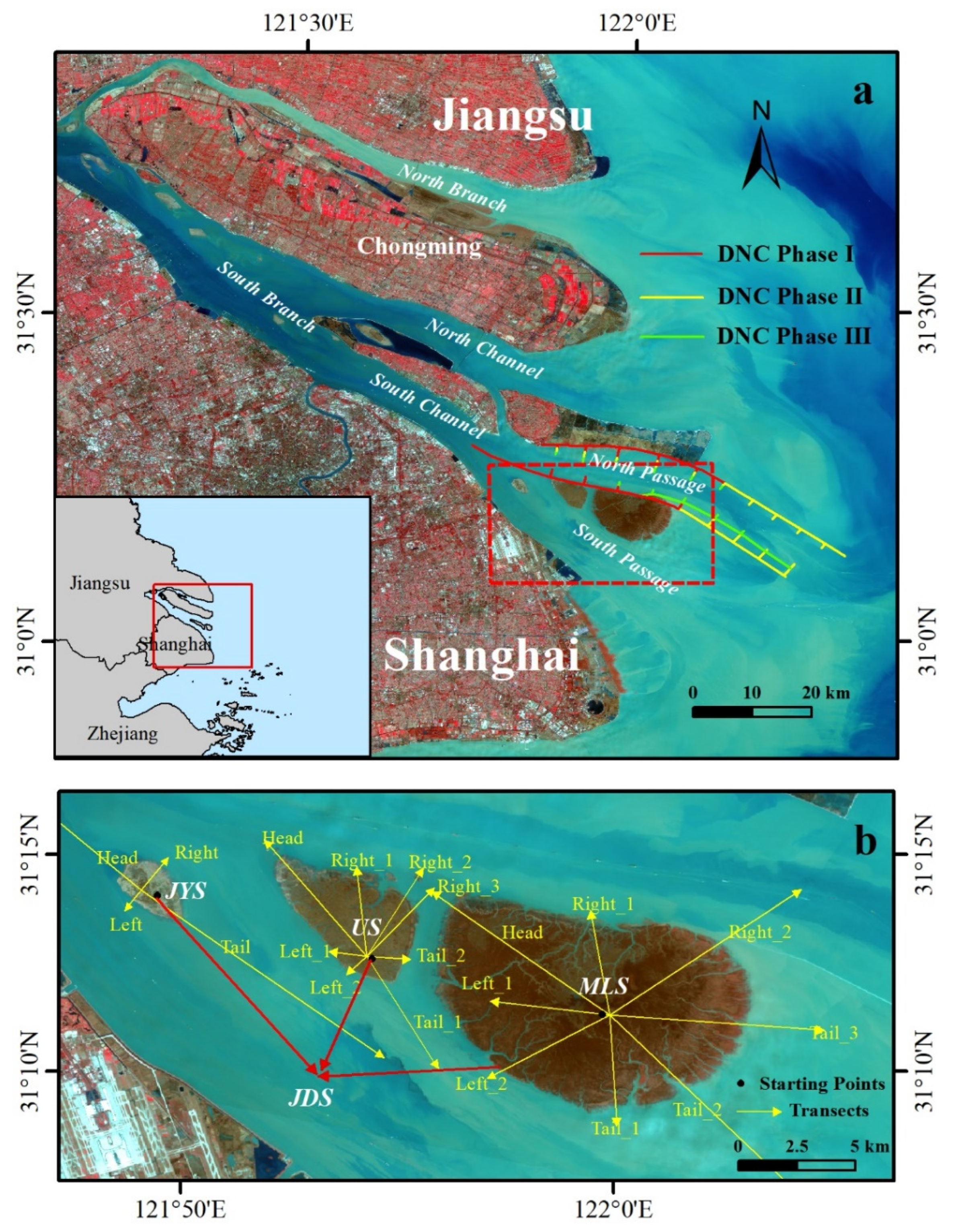
The JDS exposed since the 1950s mainly includes the Jiangya Shoal (JYS), Upper Shoal (US), Middle Shoal (MS) and Lower Shoal (LS). Since the MS and LS have been connected, hereinafter referred to as the Middle-Lower Shoals (MLS). The JDS (Figure 1b), located (31°03’–31°17’N, 121°46’–122°15’E) between South Passage (SP) and North Passage (NP), is currently the estuary shoal closest to the outer sea of the Yangtze Estuary, also the youngest estuary sandbar.
Before the implementation of the “Planting green and attracting birds” ecological engineering in 1997 [27] and the DNC project in 1998 [18], the JDS was hardly affected by human activities. To effectively protect the wetland ecosystem and natural environment of the JDS, and promote the development of the regional ecosystem, the JDS wetland was listed as a China national wetland nature reserve in 2005. So far, the JDS is uninhabited, and is also the only national protected area that basically maintains the original estuary sandbar and its development process. Therefore, research on the evolution of JDS will help reveal the evolution of estuary sand bars and sand islands.
3. Data and Methods
3.1. Satellite Data and Pre-Processing
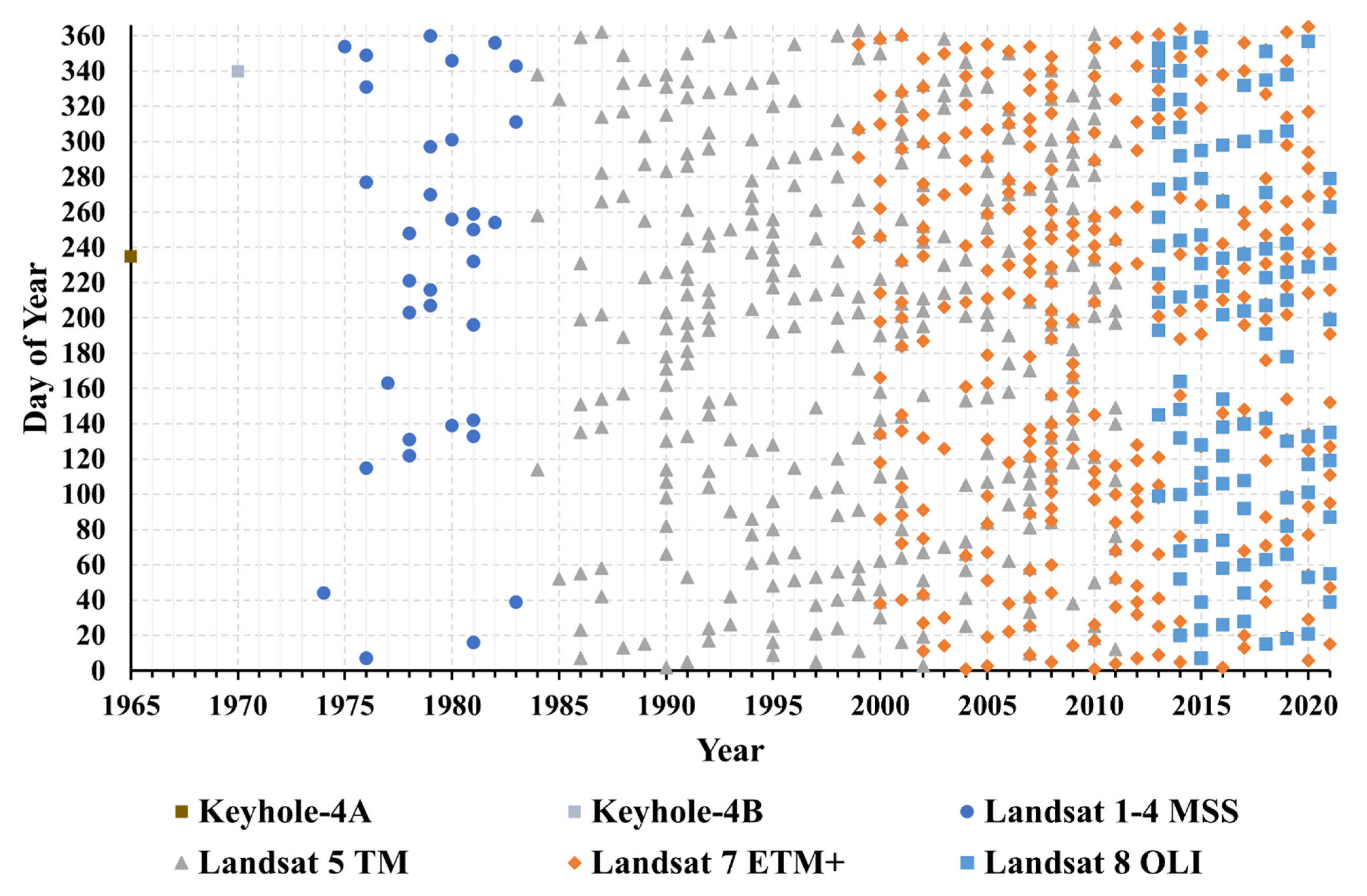
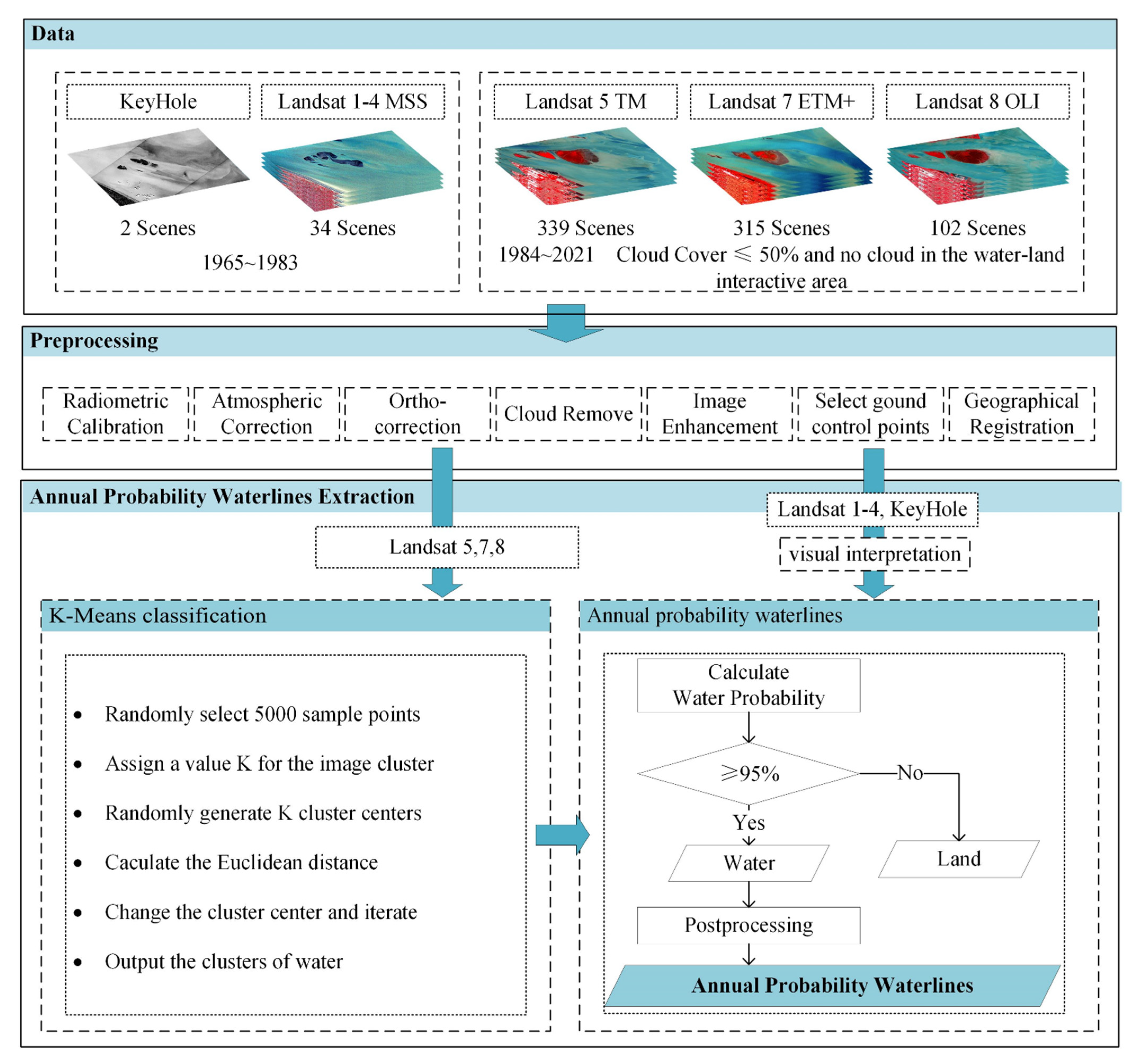
The Keyhole and the Landsat series of satellites were applied in the paper (Figure 2). The 2 Keyhole images on 23 August 1965 and 6 December 1970, were from the Keyhole-4A and Keyhole-4B satellite, respectively, which are panchromatic spectral images with the spatial resolution of 1.8 m. The applied 790 Landsat images are all multispectral images, including 34 scenes of Landsat 1–4 Multispectral Scanner (MSS) images in 1974–1983 with the spatial resolution of 78 m, 339 scenes of Landsat 5 Thematic Mapper (TM) imagery in 1984–2011, 315 scenes of Landsat 7 Enhanced Thematic Mapper Plus (ETM+) imagery in 1999–2021, 102 scenes of Landsat 8 Operational Land Imager (OLI) images in 2013–2021. The spatial resolution of Landsat 5/7/8 images are all 30 m. All available Landsat 1–8 images from the Google Earth Engine (GEE) platform during 1974–2021 with the cloud coverage less than 50% and no cloud coverage in the water-land interactive area, were all included in this paper.
Since there was no top-of-atmosphere reflectance data of Landsat 1/2/3 in the GEE platform, the coefficients stored in scene metadata were used to convert the Digital Numbers to at-sensor radiance. The surface reflectance data of Landsat 4/5/7/8 provided by GEE, which meets geometric and radiometric quality requirements, were directly employed. As for the atmospheric correction, the Landsat Ecosystem Disturbance Adaptive Processing System software was used for Landsat 4/5/7 image correction, the Land Surface Reflectance Code algorithm was used for Landsat 8 image correction [42], to generate the surface reflectance data. Furthermore, the C function of mask algorithm [43] populated cloud, cloud confidence, and cloud shadow pixels in the Landsat product processing.
3.2. Methods
Due to the influence of tide and wave fluctuations, the sea water rises and falls from time to time, the sea level is accordingly high and low, making the boundary between the ocean and the land constantly changing. Therefore, the actual coastline should be a collection of countless sea-land boundary lines between high and low tides, which spatially represents a band-like fluctuation range of a certain width rather than a line with a fixed geographical location. The remote sensing instantaneous waterline corresponds to the position of the ocean-land interface at a given time, not the position under “normal” or “average” conditions. On the long-term scale, the instantaneous waterline changes with the evolution of the tidal flat, while on the short-term scale it fluctuates with the tides and waves on the tidal flat. Long-term tidal flat evolution information and short-term tidal and wave-induced fluctuation information are therefore recorded in the historical fluctuations of the instantaneous waterlines.
As for the Keyhole and Landsat 1/2/3 images, limited by the quality of the data itself, the visual interpretation was applied to extract the waterlines. As for the Landsat 4/5/7/8 images, 5000 points of per image were randomly generated as the training samples. The K-means algorithm was then used to identify the image into 5 categories, and the 5 categories were further merged into 2 categories: water and land. It was thus possible to generate a water and land binary map. We therefore determined the annual probability waterlines by calculating the water probability value, , of each pixel in all images within a year (Equation (1)). It is the proportion of water observations in all good-quality observations with the value ranging from 0 to 1.
where and are the numbers of annual water and land observations recognized by the K-means algorithm, respectively. plus denotes the total observations each year. Pixels with ≥ 0.95 were classified as water. Therefore, the annual water and land binary map was obtained, which was further vectorized into the annual probability waterlines (Figure 3).
According to the above method for determining the position of the annual probability waterlines, we can, in a basic way, equate the position of the annual probability waterline with the position of the waterline at the low tide. Therefore, the long-term annual probability waterline data can be used to measure the change of the exposed area of the JDS at low tide [29].
4. Results
4.1. Waterlines Position Changes
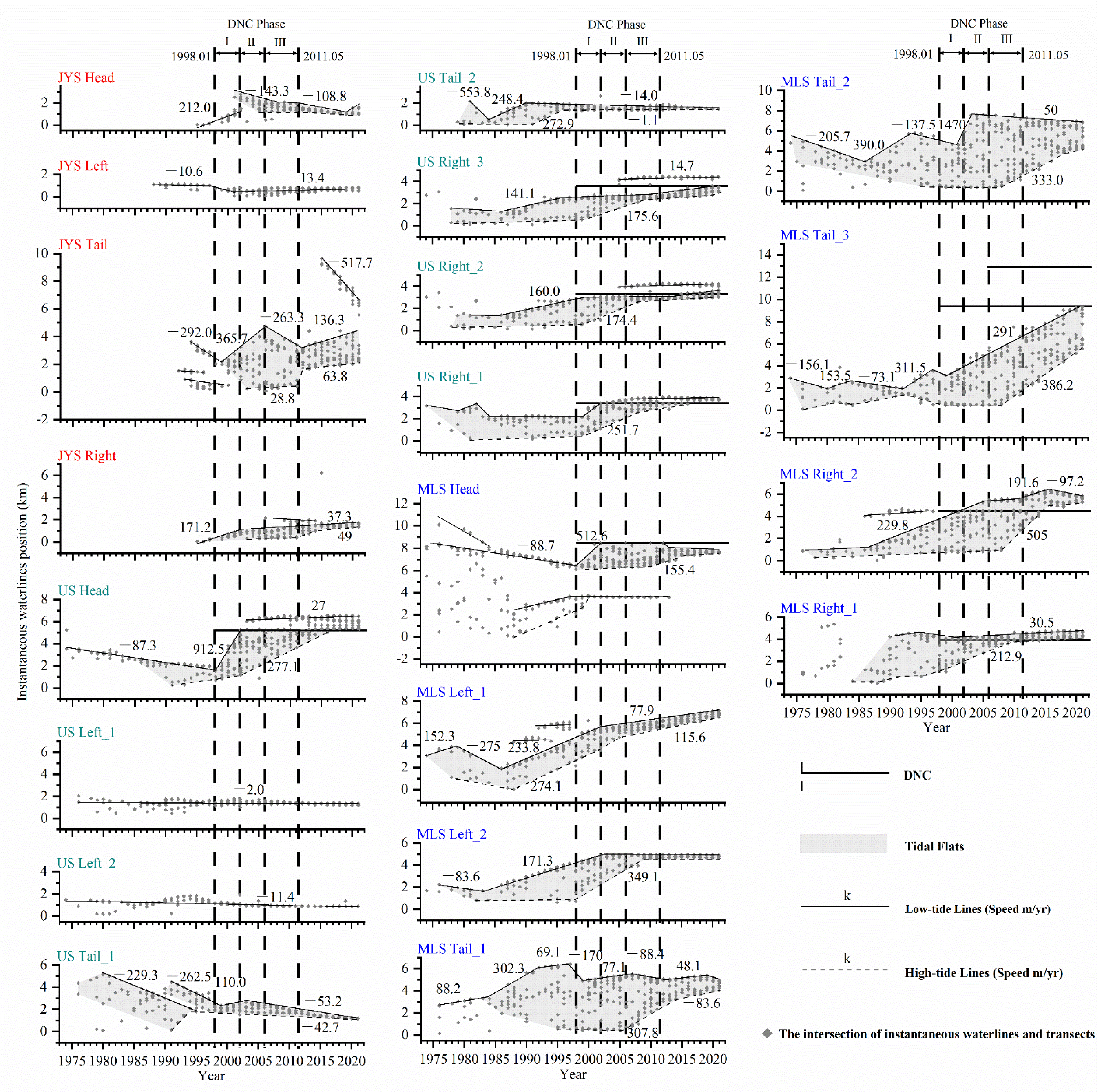
The method of focusing profile [9,26] was introduced to study the positional changes of the waterlines. A total of 20 transects were set, including 4 transects in the JYS, and 8 transects in both the US and MLS due to their significant change in recent years. Taking the centroid of the vegetation coverage area in the earliest exposed year of each shoal as the starting point, the transects were set to the head, left wing, right wing, and tail (Figure 1b). Figure 4 shows the positional change of the instantaneous waterlines during 1973–2021 in each shoal along the transects. The period 1973–2021 was chosen for two reasons. One is that remote sensing data before 1973 is limited, and only 2 Keyhole images were obtained. The amount of data is too small to carry out the fluctuation analysis of the instantaneous waterline. The other is the Keyhole images belong to reconnaissance satellite data, and the coordinate information on the data is blocked before it is publicly released. Even after geometric correction, the spatial accuracy after correction is still low due to the limited quality and number of ground control points that can be selected in the area.
Before the DNC construction in 1998, the JYS, first exposed in 1987, was in a state of natural evolution of deposition, which is characterized by the rapid deposition at the head and on the right wing, the slight erosion on the left wing, and two small sand bars merged at the tail. As for the US, the head of the low tide line retreated rapidly, then it turned to rapid deposition in the early stage of the DNC construction. The left wing was basically stable. The right wing of the low tide line silted up toward the south training jetty. The tail-2 of the low tide line was sometimes erosion and sometimes deposition, while the tail-1 was in continuous erosion. As for the MLS, the head of the low tide line gradually retreated, while the left wing eroded first since 1979, then quickly deposited. On the right wing, the low and high tide lines constantly silt up to the south training jetty, and continue to deposit around the groins. The tail_1 rapidly deposited, while the tail_2 and tail_3 were sometimes eroded and sometimes deposited.
During the DNC construction in 1998–2011, the JYS head was initially deposited and then slightly eroded. On the left wing it was slightly eroded and then basically stable. While on the right wing, the deposition speed slowed down, and the tail first showed rapidly deposition downstream and then erosion. As for the US, the head of the low tide line silted up to the south training jetty in 2004 and then basically stabilized. The tail_2 was generally stable, the tail_1 showed a trend of deposition first and then erosion. As for the MLS, the head was basically stable after silting to the south training jetty in 2002 (the DNC Phase II completed). The low tide line and high tide line of the Left_2 were basically stable from 2002 and from 2009 (after Phase II completed), respectively. The low tide line of tail_3 showed an obvious trend of deposition with the high silting rate of approximately 291 m/yr.
After the DNC construction in 2012–2021, the JYS head slightly eroded, the left and right wings slightly deposited. A small sand bar appeared at the tail in 2015, which has not yet been merged. As for the US, the low tide line and the high tide line gradually converged. The MLS of the low tide line showed a rapid deposition trend except the Tail_2 and the Right_2.
4.2. Exposed Area Changes
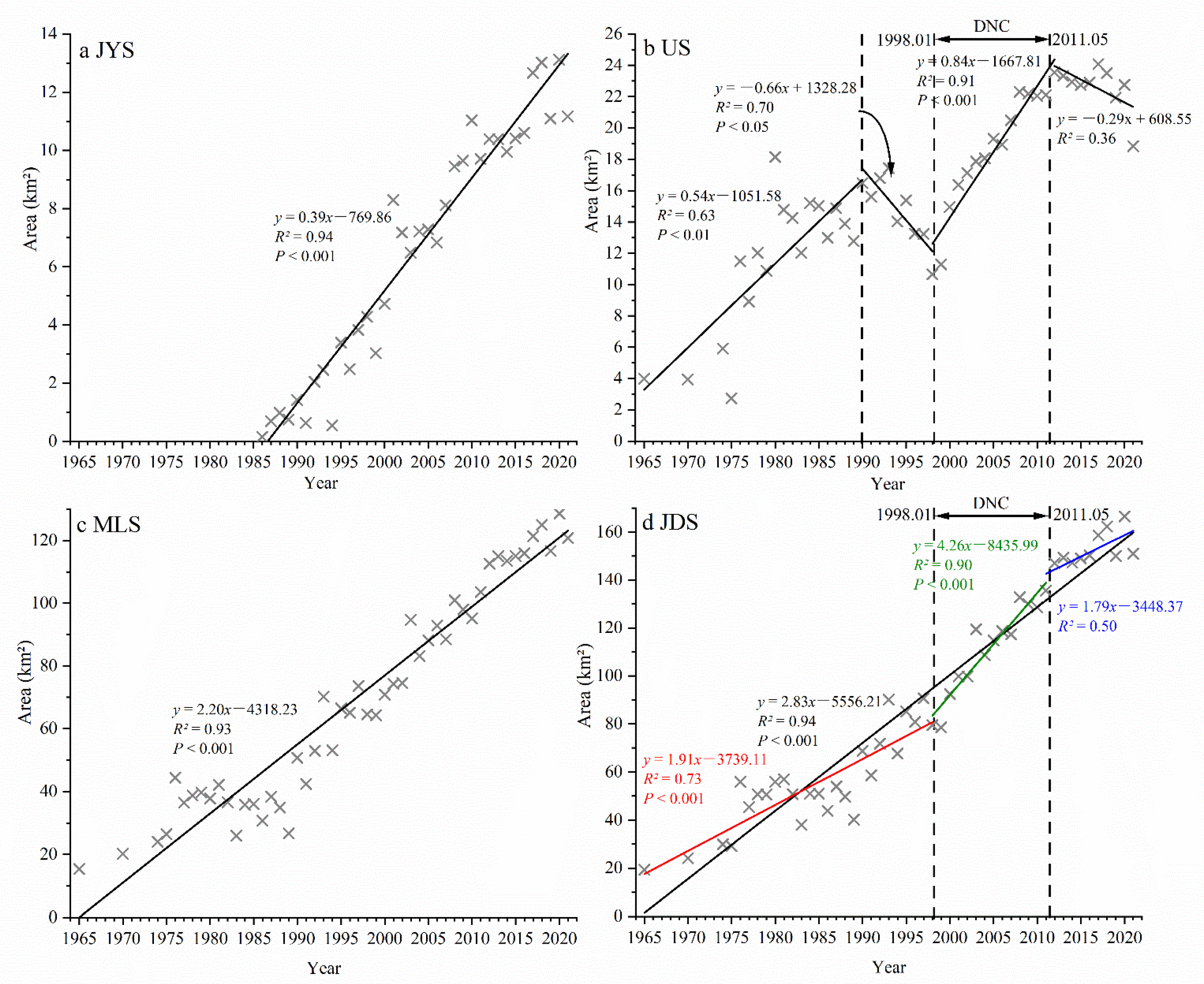
Since the formation of the JDS, statistics on the exposed area at low tide showed an overall trend of deposition and expansion during 1965–2021 (Figure 5). There was a certain fluctuation in the exposed area in some years, mainly because the water level was not completely consistent with the low tide level when the satellite image was taken.
The exposed area of the JDS showed an obvious linear increase trend (Figure 5d). The total area in 1965 was 19.32 km2, increased to 68.64 km2 in 1990, 79.50 km2 in 1998, 150.92 km2 in 2021. Among them, the exposed areas of the JYS and the MLS also showed an obvious linear increase trend with the increase rate of 0.39 km2/yr and 2.20 km2/yr, respectively. The growth rate of the MLS was nearly six times that of the JYS (Figure 5a,c). While the area of the US showed a segmented linear variation feature. That is, it showed a linear increase trend in 1965–1990 and 1998–2011 with the rate of 0.54 km2/yr and 0.84 km2/yr, respectively, and a linear decrease trend in 1991–1998 and 2012–2021 (Figure 5b).
The variation characteristics of the exposed area of JDS during 1965–2021 can be divided into three stages. For more than 30 years in the natural state during 1965–1997, the JDS showed the characteristics of steady deposition. During the DNC construction in 1998–2011, the JDS showed the characteristics of accelerated expansion. The deposition rate was 4.26 km2/yr. In the 10 years between 2012–2021, the existing project construction was basically stable without new large-scale engineering interference, the JDS maintained the trend of continuous accelerated deposition with reduced deposition rate of 1.79 km2/yr, but accompanied by local erosion (Figure 4).
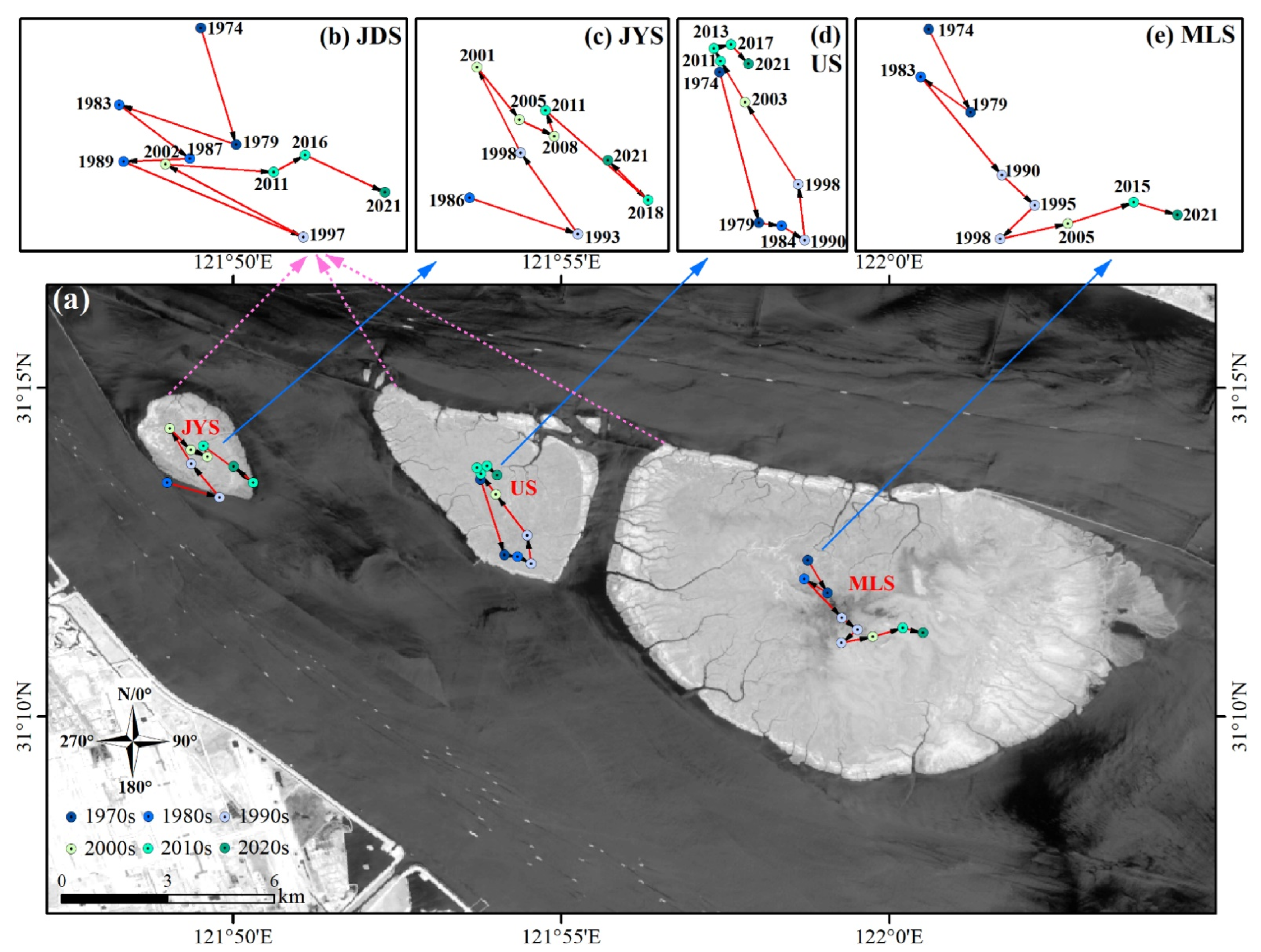
4.3. Centroid Position Changes
Based on the centroid position change analysis of the JDS annual probability waterlines, its evolution trajectory can be clearly expressed (Figure 6). We found that the JDS silted up to the southeast, showing a behavior pattern obviously related to the DNC construction (Figure 6b). Specifically, from 1974 to 1987, the centroid direction detoured, first moved to the southeast, then turned to the northwest, then back to the southeast. Since 1989–1997, the centroid moved 1.90 km to the southeast (approximately 109.36°) with an average moving speed of 238.03 m/yr (Table 1). During the implementation of the estuary project, the centroid turned back to the northwest in 1997–2002, then moved east in 2002–2011. The centroid movement rate of 304.52 m/yr in 1997–2002 dropped to 117.74 m/yr in 2002–2011. Between 2011–2021, the centroid first turned to the northeast and then to the southeast. Therefore, in the past 60 years, the centroid position of the JDS showed a trend of southward movement with westward detours before the construction of DNC started in 1998. During the construction of DNC in 1998–2011, the centroid direction first moved northwest, and then east. After the construction of DNC between 2011–2021, the JDS mainly deposited and expanded eastward.
The centroid motions in various parts of the JDS exhibited different behavioral patterns. The JYS (Figure 6c) centroid moved rapidly to the southeast from 1986 to 1993, and then turned to the northwest from 1993 to 2001, with the rate of 231.96 m/yr in 1993–1998 increased to 375.60 m/yr in 1998–2001. Then the centroid mainly turned to the southeast and reversed to the northwest in 2018–2021. As for the US (Figure 6d), the centroid moved mainly southward from 1974 to 1979, then turned eastward, and then northward. During the implementation of DNC in 1998–2011, it moved rapidly to the northwest. Especially in 1998–2003, the average moving speed reached 276.38 m/yr. After 2011, the centroid changed irregularly in a small area with the rate dropped rapidly. For the MLS (Figure 6e), the moving direction of the centroid was basically the same as that of the US in the early stage, but there were differences in the specific time points. Specifically, in 1974–1979, the MLS centroid shifted mainly to the southeast and then to the northwest. Before the DNC implementation in 1983–1995, it moved 1.92 km to the southeast. Among them in 1983–1990, the rate reached to 202.87 m/yr. From 1998 to 2021, the centroid generally moved east.
4.4. Geomorphological Changes
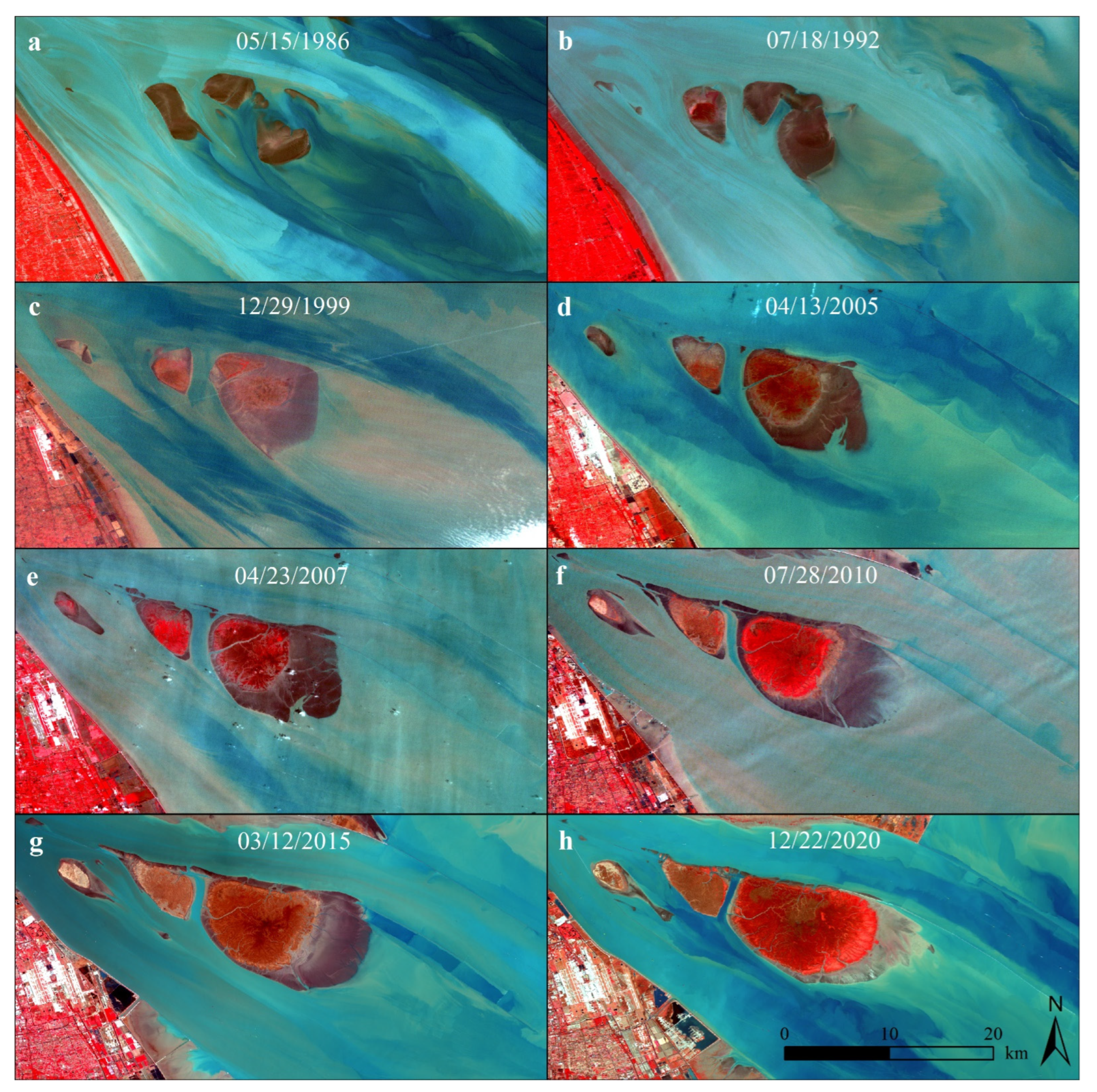
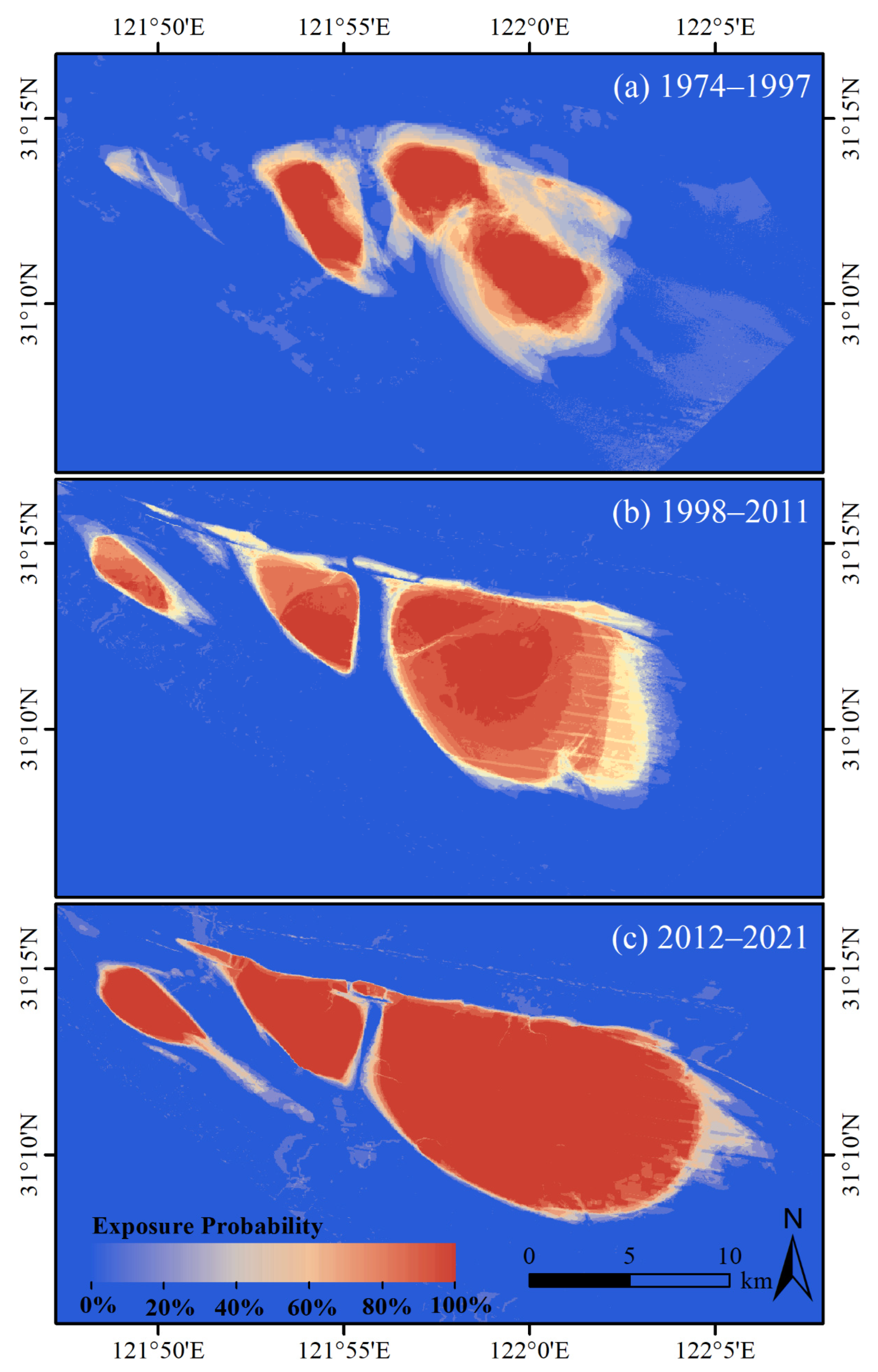
The satellite images at different acquisition times (Figure 7) and the exposure probabilities of the JDS (Figure 8) were combined to study the morphological changes of the JDS.
Before the ecological engineering of introducing salt marsh vegetation in 1997 and the construction of DNC in 1998, the JYS was a sand spit [44], and gradually separated from the mudflat under the continuous action of ebb current (Figure 8a). Then, it transformed into a heart-shaped estuarine tidal flat, and emerged steadily (Figure 7a,b and Figure 8a). The US was an approximately rounded rectangle (Figure 7a). Affected by the erosion from the SP and the tidal creek between the US and MLS, a sharp corner in the southeast direction appeared at the tail (Figure 7b). The MS and LS were in a separate state before 1986. Specifically, the MS presented a fan-shaped feature with the left wing and tail as straight lines, the head and right wing as arcs. The LS presented a rounded rectangle shape (Figure 7a and Figure 8a). It then merged (Figure 7b and Figure 8a).
During the rapid growth of salt marsh vegetation and the DNC implementation in 1998–2011, the JYS deposited towards the southeast with the head developed and widened (Figure 7c). It then evolved into a rectangular shape along the southeast direction with four smooth corners (Figure 7d). Because the south training jetty gradually narrowed and blocked the north entrance of the tidal creek between the US and MLS, the US presented an obtuse triangle with the left wing as its base (Figure 7d–f and Figure 8b), and the MLS first showed an approximate rhombus-shape, and the largest tidal creek in the northeast-southwest direction appeared at the tail (Figure 7c–e). With the continuous extension of the MLS toward the southeast, its geomorphological features changed to a spindle shape. The direction of the tidal creek changed to southeast-northwest, and its size decreased significantly (Figure 7f and Figure 8b).
After the DNC construction between 2011–2021, the JDS continued to extend southeast as a whole. Specifically, the JYS merged the newborn sand bar on the US south side (Figure 7h and Figure 8c). The head of US continued to deposit towards the northwest along the south training jetty, then it gradually changed into an approximate acute isosceles triangle with the tail as the base and the left and right wings as the two waists (Figure 7g), and the tail became straighter (Figure 7h and Figure 8c). The spindled-shape of the MLS continued to develop, and the southeast-northwest tidal creek almost disappeared. Affected by the tidal creek between the US and MLS, the arc-shape at the head of the MLS disappeared and turned into a straight shape (Figure 7f–h and Figure 8c).
5. Discussion
5.1. Sufficient High-Quality Remote Sensing Images and High-Precision Waterline Extraction
Previous studies used 2–30 remote sensing scenes over 4–40 years with an average of 0.25–1.25 scenes per year to calculate changes in the coastline erosion or deposition rates, commonly referred to as the end-point rate [45]. These relatively small numbers of remote sensing images can yield a useful but limited understanding of coastline changing processes, which are insufficient to characterize the highly dynamic changes [10]. In addition, the accuracy of coastline interpretation is often questioned, usually leading to large computational errors in the study of tidal flat evolution [46]. Zhang et al. [9] made some improvements to depictions of the JDS’s waterline position and exposed area change using an average of ten satellite images per year, which promoted our understanding of delta evolution.
Sufficient and high-quality 792 time-series remote sensing images from 1965 to 2021 were used to obtain long-term series and high temporal resolution instantaneous waterlines, which guaranteed the “dynamics” of the instantaneous waterline position, rather than the position under “normal” or “average” conditions. Therefore, the instantaneous waterline obtained in this paper reflects the tidal flat evolution information in the long-term and the tide- and wave-induced fluctuation in the short-term. The classic K-means algorithm and the statistical probability were further combined to generate the annual probability waterlines at low tide, and accordingly used to calculate the annual exposed area. This method can effectively reduce the error caused by the interpretation accuracy of the waterlines [47], quantitatively study their high dynamic change characteristics, and display more detailed information. In the case of sufficient and high-quality remote sensing image data, this method of extracting the annual probability waterline is also applicable to other regions.
The instantaneous waterline method used in this paper requires sufficient remote sensing images to ensure that the instantaneous waterlines obtained are in different tidal levels. The fluctuation of water levels over time can then be discussed. In addition, with the support of enough remote sensing data, the method used in this paper can only analyze the evolution of tidal flats from low tide (instantaneous water depth of 0 m) to high tide. As for tidal flats below water depth of 0 m, its evolution analysis needs to be supplemented with underwater topographic data.
5.2. Sediment Sources
In recent decades, the runoff of the Yangtze River was basically stable, but the sediment load experienced a rapid and stepped decline [9]. In 2006–2019, the average sediment load at Datong station remained at 1.24 × 10⁸ t/yr, which was only 27% of the average between 1953–1984. This was probably due to the water storage of more than 50,000 dams including the TGD built in the Yangtze River [22]. However, the waterlines showed a tendency of deposition, while erosion only occurred at a specific time in local areas (Figure 4, Figure 5 and Figure 7). The overall depositional trend indicated that the evolution of the JDS tidal flat was less affected by the sharp decrease in sediment from the Yangtze River. The reduction of sediment transport was not the most direct factor affecting the JDS evolution.
The sediment from the Yangtze riverine usually has a large particle size. The average particle size of the suspended sediment at Datong station increased from 8.9 μm between 2000–2006 to 15.8 μm between 2016–2019 [9,48]. The transport of a large amount of coarse riverine sediment was beneficial for the shoal growth. The sediment from outside the mouth under the action of the strong upwelling current, formed by the horn-shaped Yangtze estuary, also contributed to the shoal growth [7,9,49]. In addition, the maximum turbidity zone in the Yangtze Estuary contains the lower reaches of the north channel, the NP and SP, which is exactly where the JDS is located. Benefiting from the resuspension of the bottom sediment, the sediment supply from the outside of the estuary, and the unique flocculation effect of the largest turbidity zone, the suspended sediment concentration in the JDS did not decrease under the sharp reduction from the upstream sediment transport [9,50], which further ensured the sediment sources for the JDS growth.
The accelerated growth of the exposed area of the JDS at low tide was also related to its morphology [9,51,52]. According to the law that the spindle-shaped landform will cause its area growth rate to be one order higher than the height growth rate, the exposed area of the JDS indeed maintained accelerated growth between 1998–2011. However, in the past decade, the growth rate reduced to 1.79 km2/yr, which is 58% lower than that of 4.26 km2/yr during the DNC construction. The trend of accelerated growth at low tide no longer existed (Figure 5d).
5.3. Influence of the Nearshore Engineering
The implementation of the nearshore engineering in the Yangtze Estuary, including the DNC and Nanhui tidal flat reclamation, etc., changed the boundary conditions of the JDS, affected the dynamic characteristics of local water and sediment, and highlighted the influence of nearshore engineering on the evolution of erosion and accumulation in the JDS.
5.3.1. DNC Project
During the implementation of the DNC phase I between 1998–2002, the south training jetty blocked the Jiangya North Channel (between the JYS and the US), resulting in a significant increase in the ebb-tidal diversion ratio of the SP, which increased from 40% to about 60% [52]. This caused the main channel of the SP deepened, then induced the left wing of the JYS erosion, the head of US and MLS from original erosion to deposition (Figure 4).
Subsequently, with the DNC implementation till 2011, the south training jetty blocked the tidal creek below the middle tide of the JDS. When the rising tide went up through the tidal creek, it turned to the west and flowed over the tidal flat in front of the US or turned back to the SP [53], the diversion ratio in the SP increased and the hydrodynamic action enhanced, resulting in the erosion on the south side of the US head (Figure 7d,e). The eroded sediment from the head of JYS and US in the SP moved down with the ebb tide, and accordingly accumulated in the JYS tail and the US Tail-1, causing the tail extended to the southeast (Figure 7d). On the north side, due to the relatively weakened hydrodynamic effect of the south training jetty, the US and MLS shoal extended upstream along the north side of the submerged dykes with the trend to the north (Figure 7e,f).
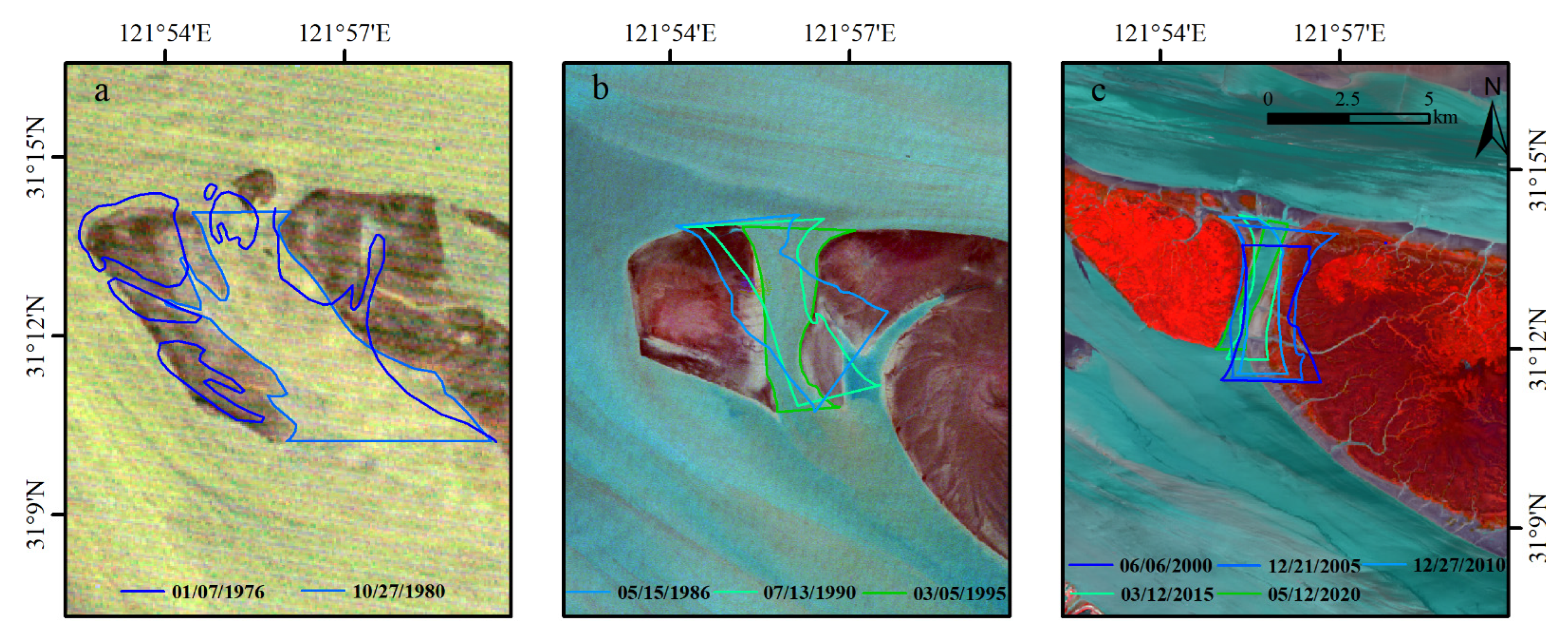
5.3.2. Project Induced Large Tidal Creek Change
The tidal creek between the US and MLS is an important channel for water and sediment exchange (Figure 9). Before the DNC construction in 1980, the area of the tidal creek was 24.63 km2 with the average width of 3.81 km. By 1995 the area reduced sharply to 7.58 km2 with the average width to 1.95 km. The direction of the tidal creek was northwest-southeast (roughly 147.1°). During the DNC construction between 1998–2011, because the channel of water and sediment from the NP entering the tidal creek was blocked, the tidal creek was further narrowed. The direction also turned to the north-south (roughly 8.8° in 2005). Subsequently, between 2012–2020 the area and width of the tidal creek continued to decrease, with the area of 2.10 km2 and the width of 0.63 km in 2020. And the direction gradually turned to the northeast-southwest (roughly 20.4° in 2020).
Erosion was evident on the southern side of the US and MLS. Especially, in the southwest of the US, the initially convex waterline gradually changed to straight and then concave (Figure 7 and Figure 9), showing the erosion stage. And the waterlines on the east and west sides of the tidal creek gradually became straight. Moreover, the southern boundary line of the tidal creek moved about 21.32 km northward from 2005 to 2015.
5.3.3. Nanhui Mudflat Reclamation
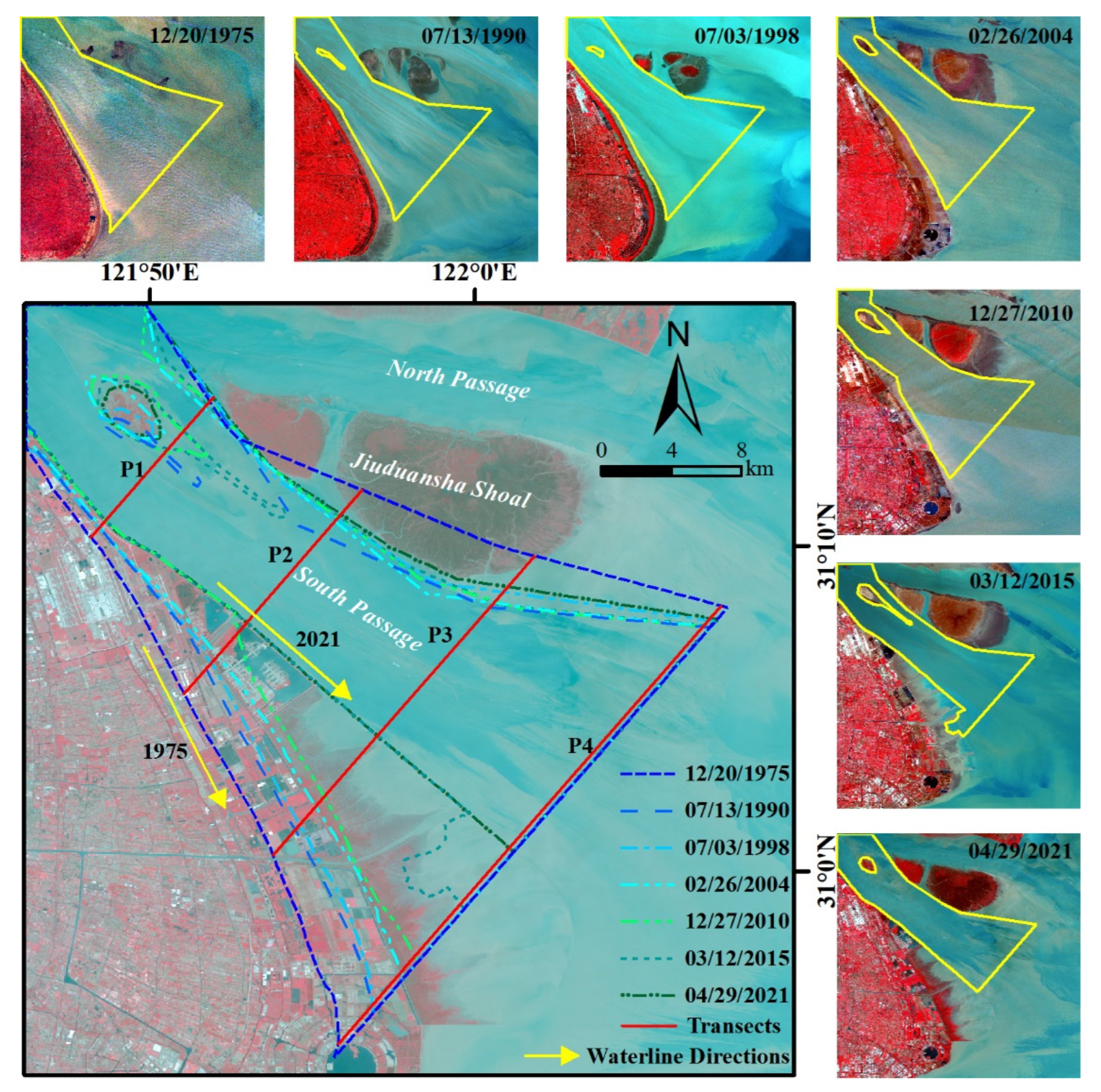
The enclosure project of the Nanhui mudflat influenced the sediment transport and hydrodynamic characteristics of the SP, thus affecting the JDS evolution. The reclamation project started in 1975, a total of about 196.07 km2 had been reclaimed by 2021 (Figure 10). The reclamation narrowed the channel width in the middle and lower sections of the SP. Taking the Nanhui waterlines on 29 April 2021, as the baseline, 4 profiles (P1, P2, P3, P4) were set on the vertical baseline with the interval of 9 km. The average width of the 4 profiles from 19.18 km in 1975 reduced to 13.48 km in 2010 to 10.85 km in 2021 (Table 2). Almost 1/2 of the width was narrowed. Zhang et al. [26] also pointed out that the reclamation of the Nanhui mudflat caused the shoreline to continuously expand towards the SP from 1978 to 2016, resulting in a sharp shrinkage of the SP width, prompting the trumpet-shaped estuary of the SP to move downstream.
In addition, the reclamation changed the direction of the coastline in the Nanhui mudflat, from 63.17° south by east in 1975 to 41.15° in 2021 (Figure 9), which was close to the direction of the downstream part of the south training jetty. This change in direction caused runoff and tidal currents to deflect northwards. In the meantime, the above factors made the water-squeeze effect of the enclosure project obvious, which enhanced the water flow in the corresponding section of the SP, resulting in the low tidal flat at the south side of the US and MLS continuously eroding and retreating to the northward.
5.4. Ecological Engineering of Vegetation Planting
In the 1960s and 1970s, the JDS was still a bare tidal flat with no vegetation. The shoal was partially exposed during low tide and submerged during high tide. In the late 1980s, the local pioneer plant began to appear. By the 1990s, there were P. australis on the high tidal flat in the US. In 1997, S. alterniflora was introduced because of its larger stem and rhizome density, which could intercept more suspended particles with smaller sizes compared with S. mariqueter. The rapidly multiplying S. alterniflora provided habitats for migratory birds and achieved rapid accumulation and expansion of tidal flats to a certain extent. The vegetation area was 6.64 km2 in 1995 and increased to 12.11 km2 under natural growth conditions by 1997 [54]. While after the ecological project was completed in 1999, the growth rate of vegetation area in those years was much higher than that in earlier years. Specifically, the average annual growth rate during 2000–2021 reached 3.95 km2/yr, which was approximately four times the rate of 1.03 km2/yr during 1990–1996. By 2021, the vegetation area increased to 104.86 km2 [54].
The rapid growth of vegetation also benefited from the growth characteristics of S. alterniflora and the clustering features of artificial introduction, that is, small patches first formed on the low tidal flats, and then merged and became larger patches sprawling toward high tidal flats and competing with native vegetation. Moreover, human disturbance restrained the competitive advantage of native vegetation. Conversely, it provided the environmental conditions for the colonization and expansion of S. alterniflora [55]. Meanwhile, a high degree of saltwater intrusion occurred in the SP after the DNC completion, resulting in the surface salinity increases in the JDS. Elevated salinity enhanced the competitive advantage of S. alterniflora, favored its better and faster growth [56], and promoted the expansion of the JDS tidal flats.
In a word, since the 1990s, the growth and succession of the JDS vegetation had an obvious effect on weakening the water flow and trapping sediment, which accelerated the expansion rate of the high tidal flat (Figure 4). Meanwhile, the superimposed sediment supply, the succession of the JDS vegetation community and the expansion of high tidal flat formed a virtuous circle of mutual promotion.
5.5. The Possible Evolution Trend in the Future
The evolution of the JDS tidal flat was the result of the combined effect of complex human activities and natural factors. As mentioned above, human activities, such as the DNC, anthropogenic reclamation, and the ecological project all had a tangible impact on tidal flat evolution. Now and in the future, the maintenance and possible further deepening of the DNC will continue to affect the evolution of the JDS tidal flat.
On the one hand, the south training jetty blocked the Jiangya North Channel and the tidal creek between the US and the MLS, forcing the development of the tidal creek at the head of the JYS, thereby enhancing the hydrodynamics of the high and ebb tide. With the merger of the JYS and the new sandbar on the south side of the US, the JYS may continue to deposit southeast in the future. On the other hand, the south training jetty and sand-retaining dikes resulted in a reduction of the cross-sectional area and flow velocity in the NP, but took an opposite effect on the SP. The changes of the tidal current and sediment distribution in the SP and NP caused more water and sediment transport through the SP, and accordingly caused the JDS to extend downstream. Considering that large-scale sediment deposition is artificially not allowed in the NP, the high tide flat of the JDS will continue to close to the south training jetty in the next short period, but will stabilize in the future.
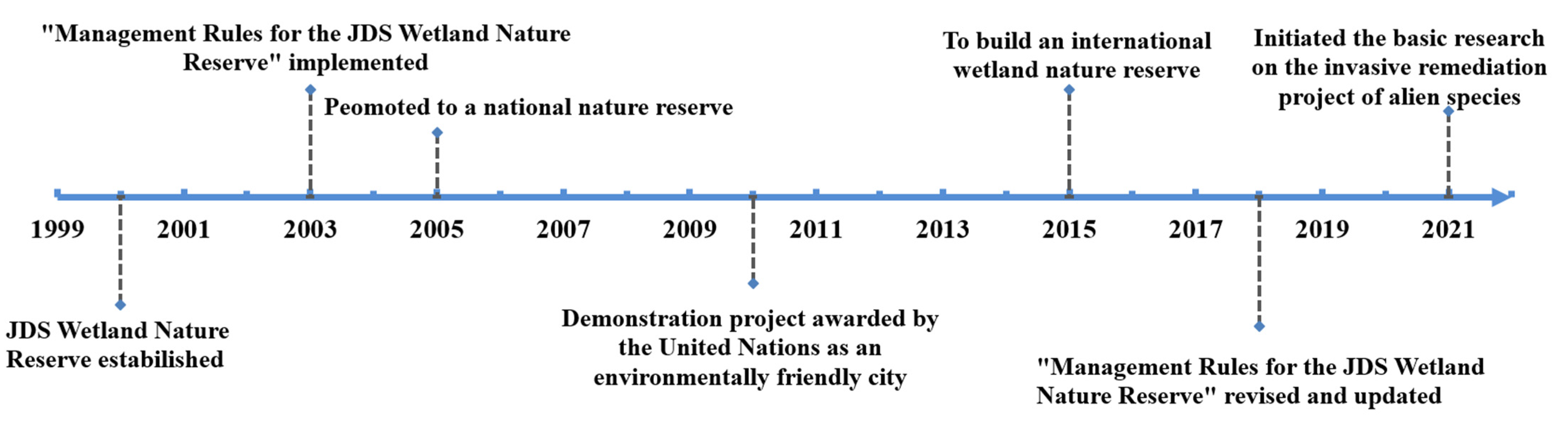
In addition to the abovementioned influential factors, a series of policies and plans issued by the local government, Shanghai Municipal Government (SMG), also had a profound impact on the JDS evolution (Figure 11). Since 2000, the SMG successively established the “JDS Wetland Nature Reserve” and issued local regulations and other documents aimed at protecting the JDS wetland. In 2005, the JDS was promoted to a national nature reserve. In the past ten years, the SMG further issued various planning schemes, such as “Administrative measures for JDS wetland national nature reserve”, “Shanghai special plan for ecological space (2018–2035)”, aiming at building a networked urban ecological pattern to strengthen the management and protect the important wetland spaces. Now, the JDS, as an important ecological barrier in Shanghai and even in the YRD region, and an important stopover site for migratory birds along the East Asian-Australian route, is becoming an “ecological business card” for Shanghai and the entire YRD.
In the light of present results, as the tidal creek between the US and MLS continues to narrow and the US and MLS will merge. The JDS tends to extend further upstream and downstream along the south training jetty. Therefore, the JDS may become more elongated in the southeast-northwest direction in the future, but its southern area will continue to erode as the SP narrowing. The ecological value of the JDS, including regional environmental value, biodiversity and the conservation value of animal and plant resources, will be higher and more important in the future, with the support of the SMG.
6. Conclusions
Based on the continuous time series of 792 satellite images, with a year frame of 1965–2021, we applied K-means classification, probability statistics, and GIS spatial analysis to extract high-precision instantaneous waterlines and annual probability waterlines. The continuous time series of geomorphological feature and position of waterlines and centroid were further determined. With the comprehensive use of the abovementioned indicators, the evolution characteristics and law of the Jiuduansha (JDS) over the past 60 years were revealed, and the underlying driving mechanism was further analyzed and discussed. The following main conclusions were drawn:
- In the past 60 years, the instantaneous waterline position of the JDS presented the characteristics of segmental and linear change;
- Except for the exposed area of the Upper Shoal (US), which showed a decreasing trend between 1992–1998 and 2011–2021, the exposed areas of each shoal and the JDS overall showed a rapid growth trend;
- During the early period between 1965–1998, the JDS presented a natural evolution state of “the head erosion, the tail deposition, and extending to the southeast”. During the recent period between 1999–2021, the evolution state changed to the engineering-dominated evolution state of “erosion on the south side, deposition on the north side, continuous extension to the southeast, and overall northward movement”;
- The accelerated deposition of JDS over the last 20 years has been mainly attributed to human activities, including the construction of Deep-water Navigation Channels and the vegetation promoting silting, followed by the upstream and downstream sediment sources;
- Current results suggest the US and the Middle-lower Shoal will merge under the continuous influence of estuary projects. The JDS would become more elongated in the southeast-northwest direction, but its south side will continue to erode. The JDS evolution should be paid attention to maintain the navigation of the deep-water channel and shoal stabilization.
Author Contributions
L.W.: Conceptualization, Writing-Reviewing and Editing. Z.Y.: Methodology, Formal analysis. W.S.: Conceptualization. Y.Z.: Project administration. L.F.: Formal analysis. B.T.: Methodology. All authors participated in the final writing—review and editing of the manuscript. All authors have read and agreed to the published version of the manuscript.
Funding
This research is supported in part by the Open Research Fund of State Key Laboratory of Estuarine and Coastal Research (No. SKLEC-KF202104), in part by the National Natural Science Foundation of China (Nos. 42176174, 42122009, 42171311), in part by the Zhejiang Provincial Natural Science Foundation of China (Nos. LY22D010002, LR19D010001) and the National Science Foundation for Post-doctoral Scientists of China (No. 2020M683258).
Data Availability Statement
All Landsat data used in this analysis can be accessed with the Google Earth Engine (https://developers.google.com/earth-engine/datasets/catalog (accessed on 1 March 2021)). The Keyhole images can be accessed with the USGS (https://earthexplorer.usgs.gov/ (accessed on 1 January 2020)).
Acknowledgments
The authors sincerely thank all anonymous reviewers and editors who provided detailed and valuable comments or suggestions to improve this manuscript.
Conflicts of Interest
The authors declare no conflict of interest.
Appendix A

Table A1.
Abbreviations and Acronyms.
| Abbreviation | Acronym | Abbreviation | Acronym | Abbreviation | Acronym |
|---|---|---|---|---|---|
| YRD | Yangtze River Delta | JYS | Jiangya Shoal | MSS | Multispectral Scanner |
| TGD | Three Gorges Dam | US | Upper Shoal | TM | Thematic Mapper |
| DNC | Deep-water Navigation Channels | MS | Middle Shoal | ETM+ | Enhanced Thematic Mapper Plus |
| SP | South Passage | LS | Lower Shoal | OLI | Operational Land Imager |
| NP | North Passage | MLS | Middle-Lower Shoals | GEE | Google Earth Engine |
References
- IPCC. Climate Change 2022: Mitigation of Climate Change; Cambridge University Press: Cambridge, UK, 2022. [Google Scholar]
- Church, J.A.; White, N.J. Sea-level rise from the late 19th to the early 21st century. Surv. Geophys. 2011, 32, 585–602. [Google Scholar] [CrossRef]
- Milliman, J.D.; Farnsworth, K.L. River Discharge to the Coastal Ocean: A Global Synthesis; Cambridge University Press: Cambridge, UK, 2011. [Google Scholar] [CrossRef]
- Anthony, E.J.; Marriner, N.; Morhange, C. Human influence and the changing geomorphology of Mediterranean deltas and coasts over the last 6000 years: From progradation to destruction phase? Earth-Sci. Rev. 2014, 139, 336–361. [Google Scholar] [CrossRef]
- Wu, W.T.; Yang, Z.Q.; Tian, B.; Huang, Y.; Zhou, Y.X.; Zhang, T. Impacts of coastal reclamation on wetlands: Loss, resilience, and sustainable management. Estuar. Coast. Shelf Sci. 2018, 210, 153–161. [Google Scholar] [CrossRef]
- Besset, M.; Anthony, E.J.; Bouchette, F. Multi-decadal variations in delta shorelines and their relationship to river sediment supply: An assessment and review. Earth-Sci. Rev. 2019, 193, 199–219. [Google Scholar] [CrossRef]
- Yang, S.L.; Luo, X.X.; Temmerman, S.; Kirwan, M.; Bouma, T.; Xu, K.H.; Zhang, S.S.; Fan, J.Q.; Shi, B.W.; Yang, H.F.; et al. Role of delta-front erosion in sustaining salt marshes under sea level rise and fluvial sediment decline. Limnol. Oceanogr. 2020, 65, 1990–2009. [Google Scholar] [CrossRef]
- Rangoonwala, A.; Jones, C.E.; Ramsey, E., III. Wetland shoreline recession in the Mississippi River Delta from petro-leum oiling and cyclonic storms. Geophys. Res. Lett. 2016, 43, 11–652. [Google Scholar] [CrossRef]
- Zhang, X.D.; Xie, R.; Fan, D.D.; Yang, Z.S.; Wang, H.M.; Wu, C.; Yao, Y.H. Sustained growth of the largest unin-habited alluvial island in the Changjiang Estuary under the drastic reduction of river discharged sediment. Sci. China Earth Sci. 2021, 64, 1687–1697. [Google Scholar] [CrossRef]
- Zhang, X.D.; Xu, K.H.; Yang, Z.S.; Tan, X.W.; Wu, C. Decreasing land growth and unique seasonal area fluctuations of two newborn Mississippi subdeltas. Geomorphology 2021, 378, 107617. [Google Scholar] [CrossRef]
- Zhao, Y.F.; Zou, X.Q.; Liu, Q.; Xu, M.; Yao, Y.L. Recent morphological changes of the Changjiang (Yangtze River) mega-delta in the Anthropocene, China: Impact from natural and anthropogenic changes. Holocene 2021, 31, 791–801. [Google Scholar] [CrossRef]
- Cao, W.Z.; Wong, M.H. Current status of coastal zone issues and management in China: A review. Environ. Ternational 2007, 33, 985–992. [Google Scholar] [CrossRef]
- Camacho-Valdez, V.; Ruiz-Luna, A.; Ghermandi, A.; Nunes, P.A. Valuation of ecosystem services provided by coastal wetlands in northwest Mexico. Ocean. Coast. Manag. 2013, 78, 1–11. [Google Scholar] [CrossRef]
- Costanza, R.; Anderson, S.J.; Sutton, P.; Mulder, K.; Mulder, O.; Kubiszewski, I.; Wang, X.T.; Liu, X.; Pérez-Maqueo, O.; Martinez, M.L.; et al. The global value of coastal wetlands for storm protection. Glob. Environ. Chang. 2021, 70, 102328. [Google Scholar] [CrossRef]
- Wu, J.G.; Huang, J.H.; Han, X.G.; Gao, X.M.; He, F.L.; Jiang, M.X.; Jiang, Z.G.; Primack, R.B.; Shen, Z.H. The three gorges dam: An ecological perspective. Front. Ecol. Environ. 2004, 2, 241–248. [Google Scholar] [CrossRef]
- Liang, Y.S.; Wang, W.; Li, H.J.; Shen, X.H.; Xu, Y.L.; Dai, J.R. The South-to-North Water Diversion Project: Effect of the water diversion pattern on transmission of Oncomelania hupensis, the intermediate host of Schistosoma japonicum in China. Parasites Vectors 2012, 5, 1–6. [Google Scholar] [CrossRef] [PubMed]
- Tan, Y.; Wang, Y.Q. Environmental migration and sustainable development in the upper reaches of the Yangtze River. Popul. Environ. 2004, 25, 613–636. [Google Scholar] [CrossRef]
- He, Q.; Wang, Y.Y.; Yu, Z.Y.; Liu, J. Sediment transport processes in deep water navigation channel, Yangtze estuary, China. Coast. Eng. 2006, 5, 3007–3018. [Google Scholar] [CrossRef]
- Li, X.; Liu, J.P.; Tian, B. Evolution of the Jiuduansha wetland and the impact of navigation works in the Yangtze Estuary, China. Geomorphology 2016, 253, 328–339. [Google Scholar] [CrossRef]
- Yang, S.L.; Belkin, I.M.; Belkina, A.I.; Zhao, Q.Y.; Zhu, J.; Ding, P.X. Delta response to decline in sediment supply from the Yangtze River: Evidence of the recent four decades and expectations for the next half-century. Estuar. Coast. Shelf Sci. 2003, 57, 689–699. [Google Scholar] [CrossRef]
- Gao, S. Modeling the growth limit of the Changjiang Delta. Geomorphology 2007, 85, 225–236. [Google Scholar] [CrossRef]
- Yang, S.L.; Milliman, J.D.; Li, P.; Xu, K. 50,000 dams later: Erosion of the Yangtze River and its delta. Glob. Planet. Chang. 2011, 75, 14–20. [Google Scholar] [CrossRef]
- Luan, H.L.; Ding, P.X.; Wang, Z.B.; Ge, J.Z.; Yang, S.L. Decadal morphological evolution of the Yangtze estuary in response to river input changes and estuarine engineering projects. Geomorphology 2016, 265, 12–23. [Google Scholar] [CrossRef]
- Tian, B.; Zhang, L.Q.; Wang, X.R.; Zhou, Y.X.; Zhang, W. Forecasting the effects of sea-level rise at Chongming Dongtan Nature Reserve in the Yangtze Delta, Shanghai, China. Ecol. Eng. 2010, 36, 1383–1388. [Google Scholar] [CrossRef]
- Wei, W.; Tang, Z.H.; Dai, Z.J.; Lin, Y.F.; Ge, Z.P.; Gao, J.J. Variations in tidal flats of the Changjiang (Yangtze) estuary during 1950s–2010s: Future crisis and policy implication. Ocean Coast. Manag. 2015, 108, 89–96. [Google Scholar] [CrossRef]
- Zhang, X.D.; Zhang, Y.X.; Zhu, L.H.; Chi, W.Q.; Yang, Z.S.; Wang, B.Y.; Lv, K.; Wang, H.M.; Lu, Z.Y. Spatial-temporal evolution of the eastern Nanhui mudflat in the Changjiang (Yangtze River) Estuary under intensified human activities. Geomorphology 2018, 309, 38–50. [Google Scholar] [CrossRef]
- Li, B.; Liao, C.H.; Zhang, X.D.; Chen, H.L.; Wang, Q.; Chen, Z.Y.; Gan, X.J.; Wu, J.H.; Zhao, B.; Ma, Z.J.; et al. Spartina alterniflora invasions in the Yangtze River estuary, China: An overview of current status and ecosystem effects. Ecol. Eng. 2009, 35, 511–520. [Google Scholar] [CrossRef]
- Shi, B.W.; Yang, S.L.; Wang, Y.P.; Li, G.C.; Li, M.L.; Li, P.; Li, C. Role of wind in erosion-accretion cycles on an estuarine mudflat. J. Geophys. Res. Ocean. 2017, 122, 193–206. [Google Scholar] [CrossRef]
- Wang, Y.; Liu, Y.; Jin, S.; Sun, C.; Wei, X. Evolution of the topography of tidal flats and sandbanks along the Jiangsu coast from 1973 to 2016 observed from satellites. ISPRS J. Photogramm. Remote Sens. 2019, 150, 27–43. [Google Scholar] [CrossRef]
- Shi, B.W.; Yang, S.L.; Wang, Y.P.; Yu, Q.; Li, M.L. Intratidal erosion and deposition rates inferred from field observations of hydrodynamic and sedimentary processes: A case study of a mudflat–saltmarsh transition at the Yangtze delta front. Cont. Shelf Res. 2014, 90, 109–116. [Google Scholar] [CrossRef]
- Choi, J.K.; Ryu, J.H.; Lee, Y.K.; Yoo, H.R.; Woo, H.J.; Kim, C.H. Quantitative estimation of intertidal sediment characteristics using remote sensing and GIS. Estuar. Coast. Shelf Sci. 2010, 88, 125–134. [Google Scholar] [CrossRef]
- Jiang, C.J.; Li, J.F.; de Swart, H.E. Effects of navigational works on morphological changes in the bar area of the Yangtze Estuary. Geomorphology 2012, 139–140, 205–219. [Google Scholar] [CrossRef]
- Zheng, J.H.; Peng, Y.X.; Zhang, C.; Ju, Y. Recent evolution of Jiuduansha Shoal in Yangtze Estuary and its corresponding to engineering projects. J. Coast. Res. 2013, 65, 1259–1264. [Google Scholar] [CrossRef]
- Ryu, J.H.; Kim, C.H.; Lee, Y.K.; Won, J.S.; Chun, S.S.; Lee, S. Detecting the intertidal morphologic change using satellite data. Estuar. Coast. Shelf Sci. 2008, 78, 623–632. [Google Scholar] [CrossRef]
- Yang, Z.H.; Wang, L.H.; Sun, W.W.; Xu, W.X.; Tian, B.; Zhou, Y.X.; Yang, G.; Chen, C. A New Adaptive Remote Sensing Extraction Algorithm for Complex Muddy Coast Waterline. Remote Sens. 2022, 14, 861. [Google Scholar] [CrossRef]
- Heygster, G.; Dannenberg, J.; Notholt, J. Topographic mapping of the German tidal flats analyzing SAR images with the waterline method. IEEE Trans. Geosci. Remote Sens. 2010, 48, 1019–1030. [Google Scholar] [CrossRef]
- Kang, Y.Y.; Ding, X.R.; Xu, F.; Zhang, C.K.; Ge, X.P. Topographic mapping on large-scale tidal flats with an iterative approach on the waterline method. Estuar. Coast. Shelf Sci. 2017, 190, 11–22. [Google Scholar] [CrossRef]
- Zhou, Y.Y.; Huang, H.Q.; Nanson, G.C.; Huang, C.; Liu, G.H. Progradation of the Yellow (Huanghe) River Delta in response to the implementation of a basin- scale water regulation program. Geomorphology 2015, 243, 65–74. [Google Scholar] [CrossRef]
- Cao, W.T.; Zhou, Y.Y.; Li, R.; Li, X.C. Mapping changes in coastlines and tidal flats in developing islands using the full time series of Landsat images. Remote Sens. Environ. 2020, 239, 111665. [Google Scholar] [CrossRef]
- Murray, N.J.; Clemens, R.S.; Phinn, S.R.; Possingham, H.P.; Fuller, R.A. Tracking the rapid loss of tidal wetlands in the Yellow Sea. Front. Ecol. Environ. 2014, 12, 267–272. [Google Scholar] [CrossRef]
- Sagar, S.; Roberts, D.; Bala, B.; Lymburner, L. Extracting the intertidal extent and topography of the Australian coastline from a 28 year time series of Landsat observations. Remote Sens. Environ. 2017, 195, 153–169. [Google Scholar] [CrossRef]
- Chander, G.; Markham, B.L.; Helder, D.L. Summary of current radiometric calibration coefficients for Landsat MSS, TM, ETM+, and EO-1 ALI sensors. Remote Sens. Environ. 2009, 113, 893–903. [Google Scholar] [CrossRef]
- Foga, S.; Scaramuzza, P.L.; Guo, S.; Zhu, Z.; Dilley Jr, R.D.; Beckmann, T.; Schmidt, G.L.; Dwyer, J.L.; Hughes, M.J.; Laue, B. Cloud detection algorithm comparison and validation for operational Landsat data products. Remote Sens. Environ. 2017, 194, 379–390. [Google Scholar] [CrossRef]
- Chen, Z.; Liu, L. Recent river regime evolution and navigation-obstructing characteristics of Jiangya south shoal in South Passage of the Yangtze estuary. Port Waterw. Eng. 2018, 3, 99–105, (In Chinese with English Abstract). [Google Scholar] [CrossRef]
- Thieler, E.R.; Himmelstoss, E.A.; Zichichi, J.L.; Ergul, A. The Digital Shoreline Analysis System (DSAS) Version 4.0-an ArcGIS Extension for Calculating Shoreline Change (No. 2008-1278); U.S. Geological Survey: Reston, VA, USA, 2009. [CrossRef]
- Almonacid-Caballer, J.; Sánchez-García, E.; Pardo-Pascual, J.E.; Balaguer-Beser, A.A.; Palomar-Vázquez, J. Evaluation of annual mean shoreline position deduced from Landsat 465 imagery as a mid-term coastal evolution indicator. Mar. Geol. 2016, 372, 79–88. [Google Scholar] [CrossRef]
- Salameh, E.; Frappart, F.; Turki, I.; Laignel, B. Intertidal topography mapping using the waterline method from Sentinel-1 &-2 images: The examples of Arcachon and Veys Bays in France. ISPRS J. Photogramm. Remote Sens. 2020, 163, 98–120. [Google Scholar] [CrossRef]
- Dai, Z.J.; Fagherazzi, S.; Mei, X.F.; Gao, J.J. Decline in suspended sediment concentration delivered by the Changjiang (Yangtze) River into the East China Sea between 1956 and 2013. Geomorphology 2016, 268, 123–132. [Google Scholar] [CrossRef]
- Yang, S.L. Sedimentation on a growing intertidal island in the Yangtze River mouth. Estuar. Coast. Shelf Sci. 1999, 49, 401–410. [Google Scholar] [CrossRef]
- Dai, Z.J.; Liu, J.T.; Wei, W.; Chen, J.Y. Detection of the Three Gorges Dam influence on the Changjiang (Yangtze River) submerged delta. Sci. Rep. 2014, 4, 6600. [Google Scholar] [CrossRef]
- Kang, Y.; He, J.; Wang, B.; Lei, J.; Wang, Z.; Ding, X. Geomorphic Evolution of Radial Sand Ridges in the South Yellow Sea Observed from Satellites. Remote Sens. 2022, 14, 287. [Google Scholar] [CrossRef]
- Zhan, C.; Yu, J.; Wang, Q.; Li, Y.; Zhou, D.; Xing, Q.; Chu, X. The evolutionary process of the geomorphology of tidal embayments in southern Jiaodong Peninsula, China. Estuar. Coast. Shelf Sci. 2017, 194, 182–191. [Google Scholar] [CrossRef]
- Mao, Z.C.; Guo, J.Q. Study on the collapse of upper Jiuduansha shoal and the effect of out-bar and inner channel. Ocean Eng. 2015, 33, 107–112, (In Chinese with English Abstract). [Google Scholar] [CrossRef]
- Yang, Z.H. Research on the Evolution of Erosion and Deposition in Jiuduansha of the Yangtze Estuary in the Past 60 Years Based on Remote Sensing Technology. Master’s Thesis, Chengdu University of Information Technology, Chengdu, China, 2022. [Google Scholar]
- Liu, M.Y.; Li, H.Y.; Li, L.; Man, W.D.; Jia, M.M.; Wang, Z.M.; Lu, C.Y. Monitoring the invasion of Spartina alterniflora using multi-source high-resolution imagery in the Zhangjiang Estuary, China. Remote Sens. 2017, 9, 539. [Google Scholar] [CrossRef]
- Peng, Z.Y.; Jiang, X.Z.; Hou, L.J.; He, Q. Comparison of suspended sediment and salinity profile characteristics of the maximum turbidity zone in the Yangtze estuary during the dry season in 1982 and 2012. Mar. Geol. Front. 2020, 36, 7–18, (In Chinese with English Abstract). [Google Scholar] [CrossRef]
Figure 1.
Location of the study area in the Yangtze Estuary. (a) Deep-water Navigation Channel project (DNC) in the North Passage. (b) Location of the 20 transects. The underlying image is a composite of 5-4-3 bands of the Landsat8 OLI data acquired on 22 February 2020.
Figure 1.
Location of the study area in the Yangtze Estuary. (a) Deep-water Navigation Channel project (DNC) in the North Passage. (b) Location of the 20 transects. The underlying image is a composite of 5-4-3 bands of the Landsat8 OLI data acquired on 22 February 2020.

Figure 2.
Acquisition dates and sensor types of the satellite images used in this study. The temporal resolution of Keyhole is irregular. As for the Landsat 1–3 and Landsat 4–8 images, the temporal resolution are 18 days, and 16 days, respectively.
Figure 2.
Acquisition dates and sensor types of the satellite images used in this study. The temporal resolution of Keyhole is irregular. As for the Landsat 1–3 and Landsat 4–8 images, the temporal resolution are 18 days, and 16 days, respectively.

Figure 3.
Framework of the annual probability waterlines extraction.

Figure 4.
Positional change of the instantaneous waterlines in each shoal of the JDS along the transects during 1973–2021.
Figure 4.
Positional change of the instantaneous waterlines in each shoal of the JDS along the transects during 1973–2021.

Figure 5.
Exposed area variation of low tidal flats in (a) the JYS, (b) the US, (c) the MLS and (d) the JDS.
Figure 5.
Exposed area variation of low tidal flats in (a) the JYS, (b) the US, (c) the MLS and (d) the JDS.

Figure 6.
Centroid changes of the annual probability waterlines in each shoal (a), in the JDS (b). Zoom-in views for the JYS (c), the US (d) and the MLS (e).
Figure 6.
Centroid changes of the annual probability waterlines in each shoal (a), in the JDS (b). Zoom-in views for the JYS (c), the US (d) and the MLS (e).

Figure 7.
Landsat TM, ETM+ and OLI images of the JDS at similar low tidal levels from 1986 to 2020. The image acquired on (a) 15 May 1986, (b) 18 July 1992, (c) 29 December 1999, (d) 13 April 2005, (e) 23 April 2007, (f) 28 July 2010, (g) 12 March 2015 and (h) 22 December 2020, respectively.
Figure 7.
Landsat TM, ETM+ and OLI images of the JDS at similar low tidal levels from 1986 to 2020. The image acquired on (a) 15 May 1986, (b) 18 July 1992, (c) 29 December 1999, (d) 13 April 2005, (e) 23 April 2007, (f) 28 July 2010, (g) 12 March 2015 and (h) 22 December 2020, respectively.

Figure 8.
Exposure probability of the JDS in satellite images from (a) 1974–1997, (b) 1998–2011 and (c) 2012–2021.
Figure 8.
Exposure probability of the JDS in satellite images from (a) 1974–1997, (b) 1998–2011 and (c) 2012–2021.

Figure 9.
Evolution of the tidal creek between the US and MLS. The underlying image is the Landsat image acquired on (a) 27 October 1980, (b) 5 March 1995, and (c) 12 May 2020, respectively.
Figure 9.
Evolution of the tidal creek between the US and MLS. The underlying image is the Landsat image acquired on (a) 27 October 1980, (b) 5 March 1995, and (c) 12 May 2020, respectively.

Figure 10.
Evolution of the South Passage Trumpet-shape during 1975–2021.

Figure 11.
Major policies and plans issued regarding the JDS since 2000.

Table 1.
Variation in the centroid orientation and speed of annual instantaneous waterlines.
| Shoal | Time | Direction (°) | Speed(m/yr) | Shoal | Time | Direction (°) | Speed(m/yr) |
|---|---|---|---|---|---|---|---|
| JDS | 1974–1979 | 160.06 | 236.85 | US | 1974–1979 | 162.56 | 438.58 |
| 1979–1983 | 285.82 | 300.96 | 1979–1984 | 96.71 | 65.39 | ||
| 1983–1987 | 122.77 | 217.25 | 1984–1990 | 117.90 | 63.41 | ||
| 1987–1989 | 267.47 | 324.38 | 1990–1998 | 351.98 | 99.09 | ||
| 1989–1997 | 109.36 | 238.03 | 1998–2003 | 322.43 | 276.38 | ||
| 1997–2002 | 293.93 | 304.52 | 2003–2011 | 324.57 | 84.45 | ||
| 2002–2011 | 93.09 | 117.74 | 2011–2013 | 327.99 | 100.66 | ||
| 2011–2016 | 64.89 | 69.46 | 2013–2017 | 78.69 | 61.12 | ||
| 2016–2021 | 111.32 | 171.61 | 2017–2021 | 132.71 | 121.15 | ||
| JYS | 1986–1993 | 105.55 | 190.24 | MLS | 1974–1979 | 148.93 | 207.20 |
| 1993–1998 | 320.13 | 231.96 | 1979–1983 | 300.68 | 170.75 | ||
| 1998–2001 | 328.57 | 375.60 | 1983–1990 | 135.59 | 202.87 | ||
| 2001–2005 | 136.06 | 197.88 | 1990–1995 | 127.57 | 99.73 | ||
| 2005–2008 | 111.57 | 150.28 | 1995–1998 | 229.64 | 178.67 | ||
| 2008–2011 | 337.83 | 105.70 | 1998–2005 | 78.55 | 110.49 | ||
| 2011–2018 | 126.21 | 227.05 | 2005–2015 | 74.05 | 77.32 | ||
| 2018–2021 | 309.35 | 219.44 | 2015–2021 | 103.24 | 83.97 |
Table 2.
Changes in the width of the South Passage (km).
| Satellite Date | 20 December 1975 | 13 July 1990 | 3 July 1998 | 26 February 2004 | 27 December 2010 | 12 March 2015 | 29 April 2021 | |
|---|---|---|---|---|---|---|---|---|
| Profiles | ||||||||
| P1 | 9.68 | 9.12 | 9.26 | 8.45 | 8.40 | 8.26 | 8.80 | |
| P2 | 14.50 | 9.45 | 10.22 | 9.56 | 8.14 | 7.50 | 7.68 | |
| P3 | 21.31 | 15.84 | 16.58 | 14.49 | 13.90 | 9.50 | 10.59 | |
| P4 | 31.23 | 26.91 | 27.35 | 24.63 | 23.47 | 19.82 | 16.34 | |
| Average | 19.18 | 15.33 | 15.85 | 14.28 | 13.48 | 11.27 | 10.85 | |
Publisher’s Note: MDPI stays neutral with regard to jurisdictional claims in published maps and institutional affiliations. |
© 2022 by the authors. Licensee MDPI, Basel, Switzerland. This article is an open access article distributed under the terms and conditions of the Creative Commons Attribution (CC BY) license (https://creativecommons.org/licenses/by/4.0/).
Share and Cite
MDPI and ACS Style
Wang, L.; Yang, Z.; Sun, W.; Fan, L.; Tan, B.; Zhou, Y. Detailed Processes of Tidal Flat Geomorphology Evolution Based on Time-Series Satellite Images. Remote Sens. 2022, 14, 4341. https://0-doi-org.brum.beds.ac.uk/10.3390/rs14174341
AMA Style
Wang L, Yang Z, Sun W, Fan L, Tan B, Zhou Y. Detailed Processes of Tidal Flat Geomorphology Evolution Based on Time-Series Satellite Images. Remote Sensing. 2022; 14(17):4341. https://0-doi-org.brum.beds.ac.uk/10.3390/rs14174341
Chicago/Turabian StyleWang, Lihua, Ziheng Yang, Weiwei Sun, Li Fan, Benhua Tan, and Yunxuan Zhou. 2022. "Detailed Processes of Tidal Flat Geomorphology Evolution Based on Time-Series Satellite Images" Remote Sensing 14, no. 17: 4341. https://0-doi-org.brum.beds.ac.uk/10.3390/rs14174341
Note that from the first issue of 2016, this journal uses article numbers instead of page numbers. See further details here.