
Multiple Characteristics of Precipitation Inferred from Wind Profiler Radar Doppler Spectra
 , , ,
, , ,
Abstract
:1. Introduction
2. Field Campaign and Instrumentation
2.1. Cerdanya-2017 Field Campaign
2.2. UHF Wind Profiler
2.3. Micro Rain Radar
2.4. Disdrometer
2.5. Automatic Weather Stations
3. Data Processing
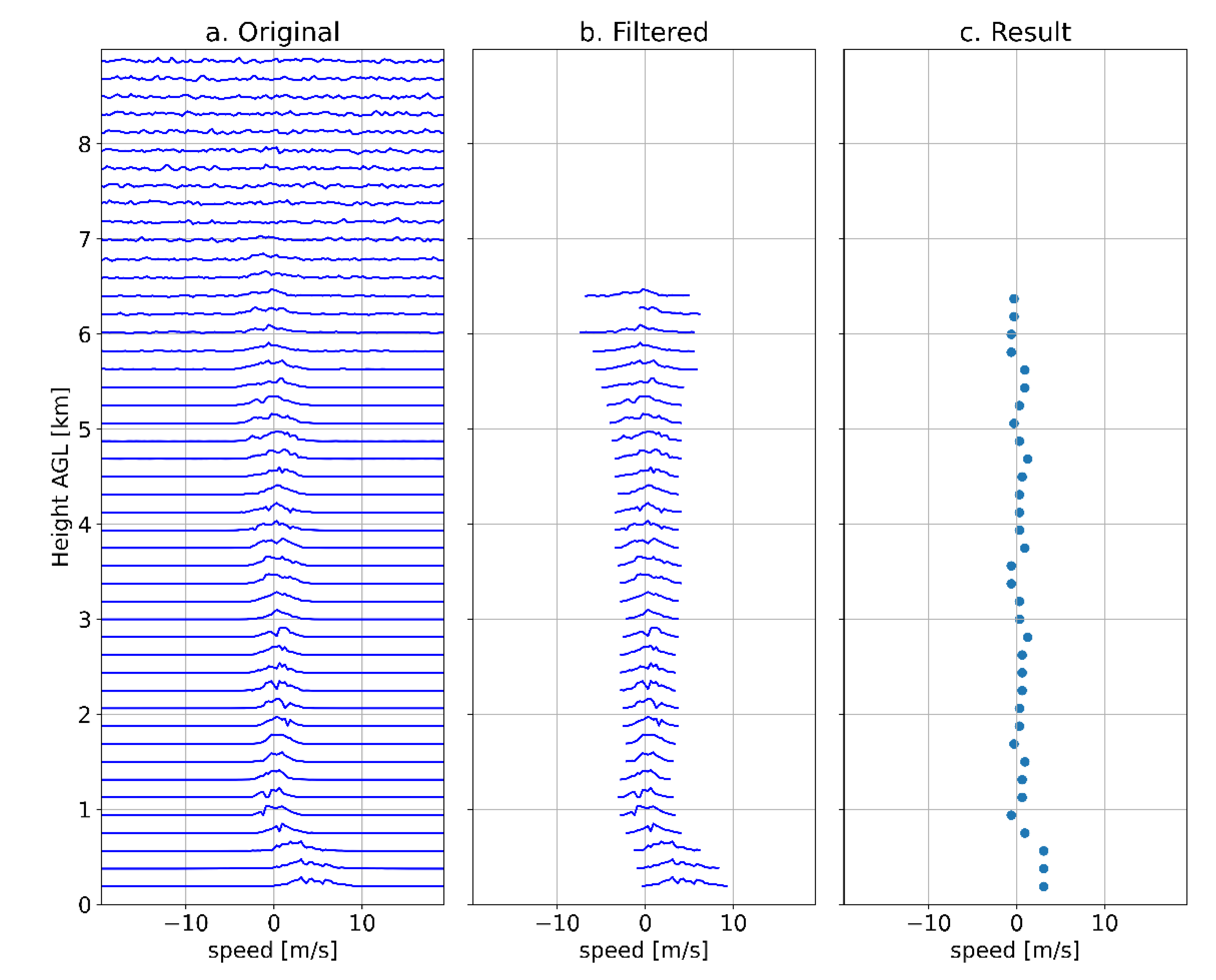
3.1. Signal Peak Detection
3.2. Vertical Continuity Check
3.3. Parameters Calculation
3.3.1. Wind Components
3.3.2. Radar Reflectivity
3.3.3. Precipitation Type
3.3.4. Drop Size Distribution
3.3.5. Liquid Water Content
3.3.6. Kinetic Energy Flux
4. Results
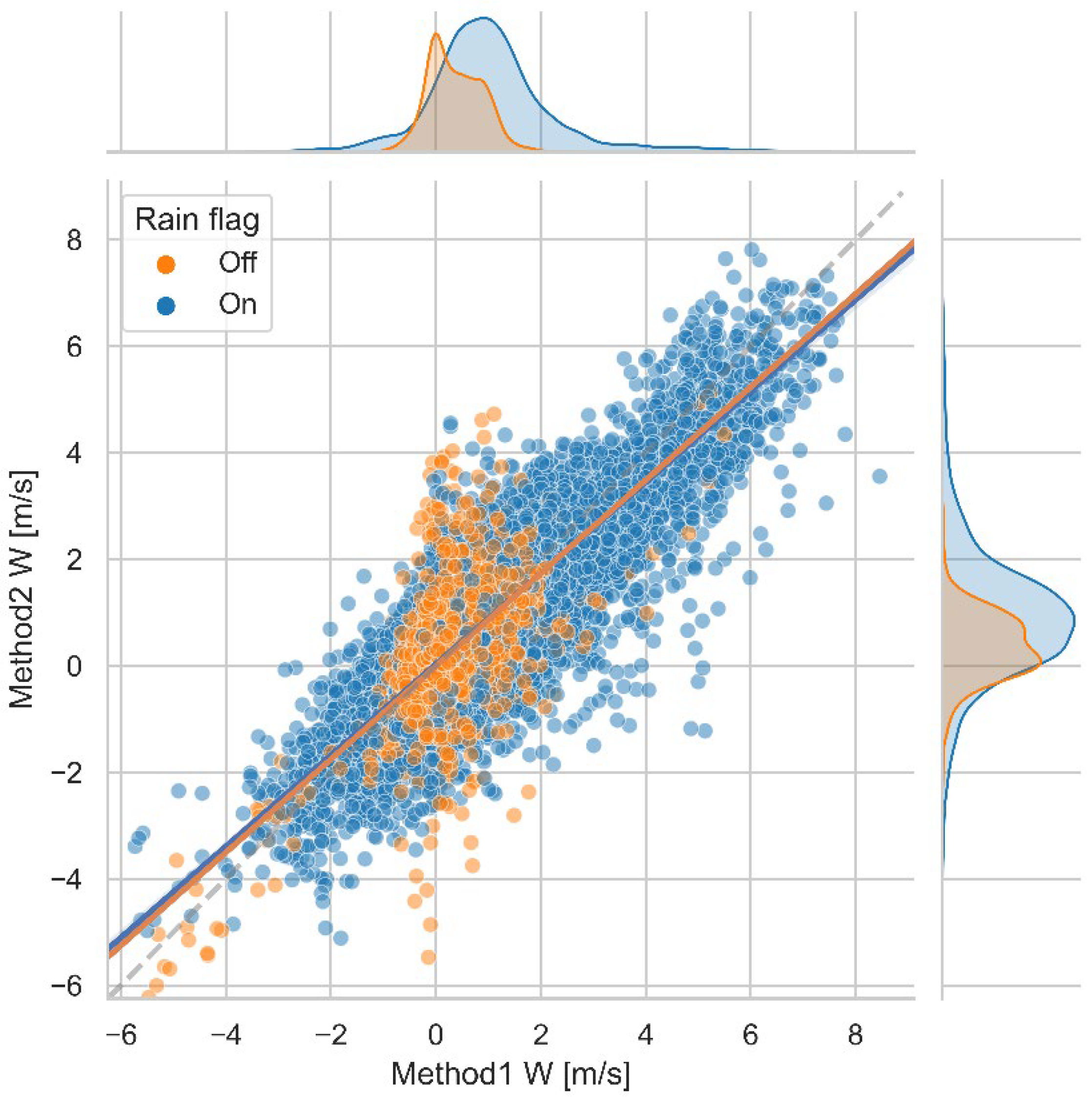
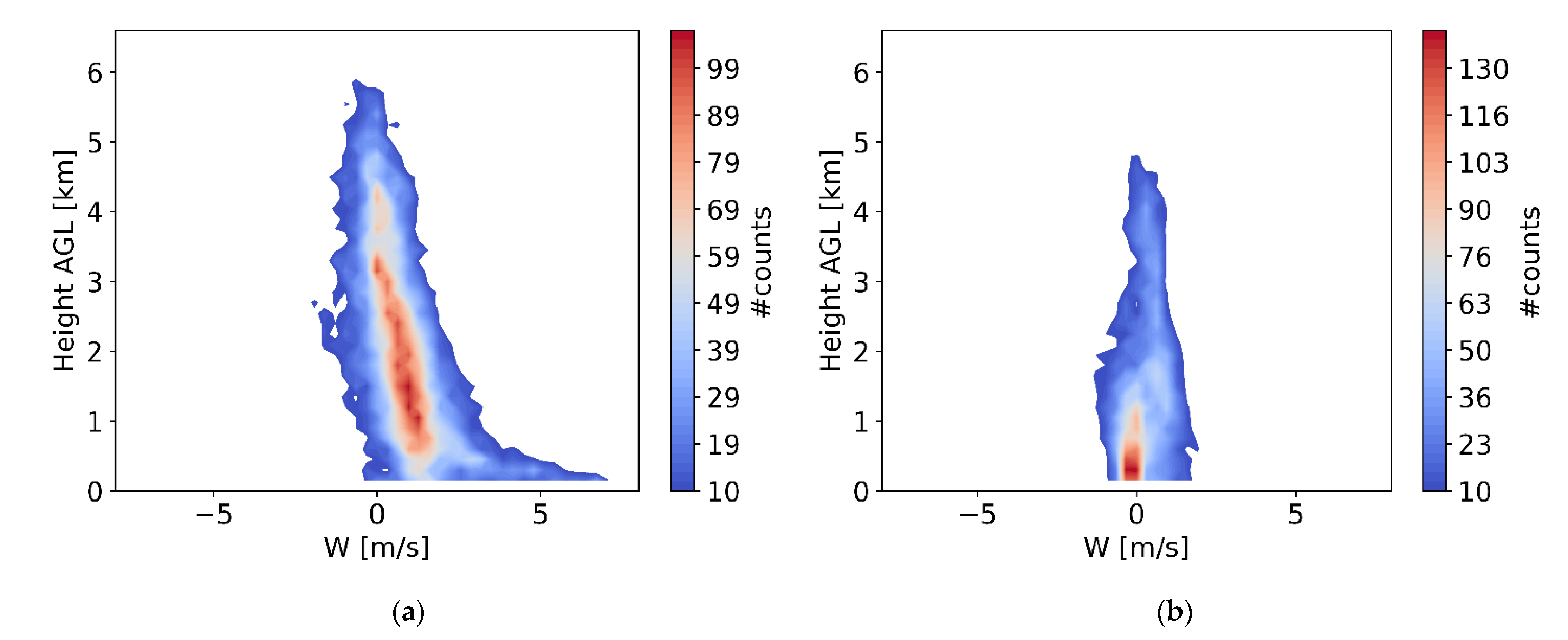
4.1. Vertical Speed
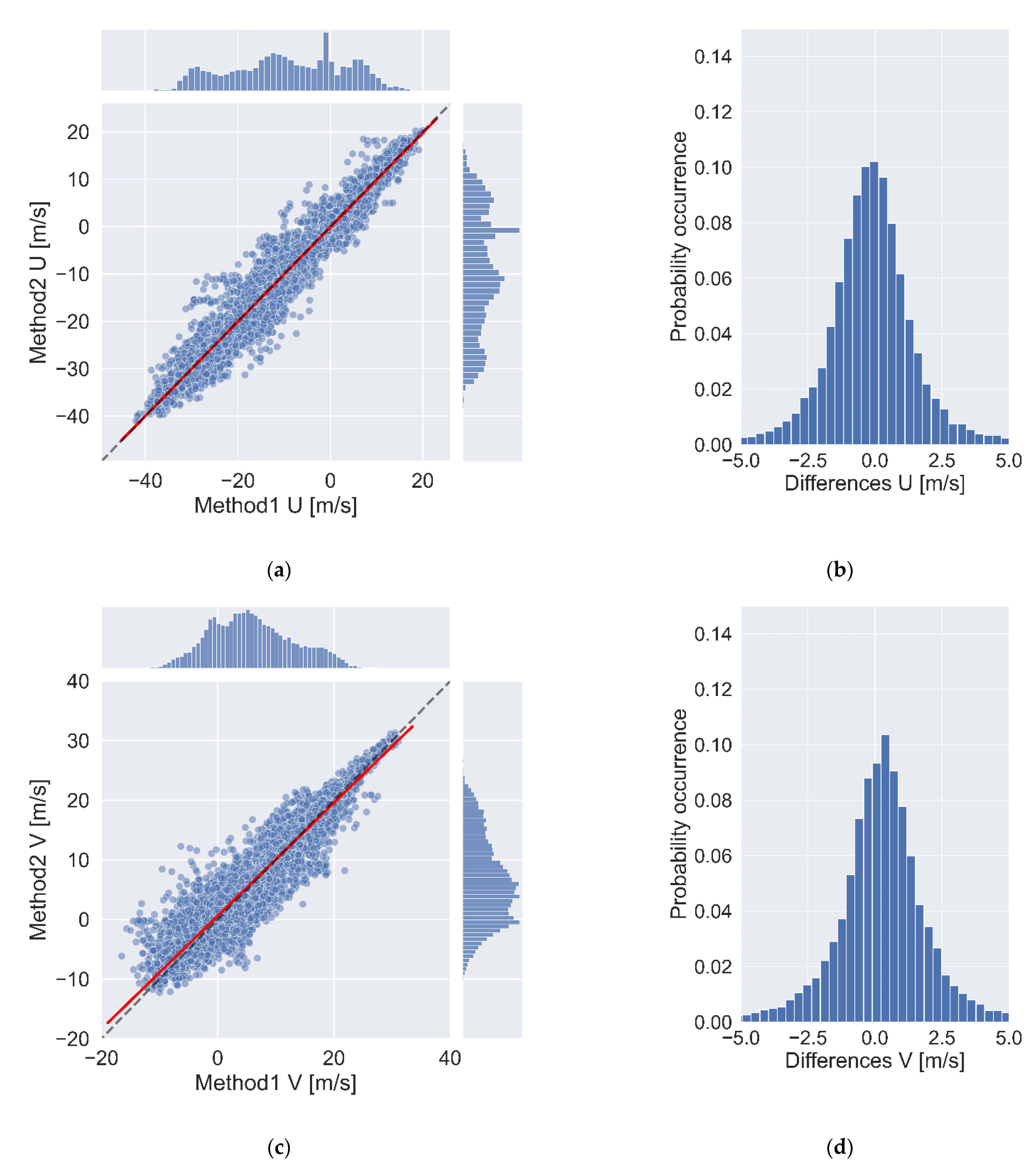
4.2. Horizontal Wind
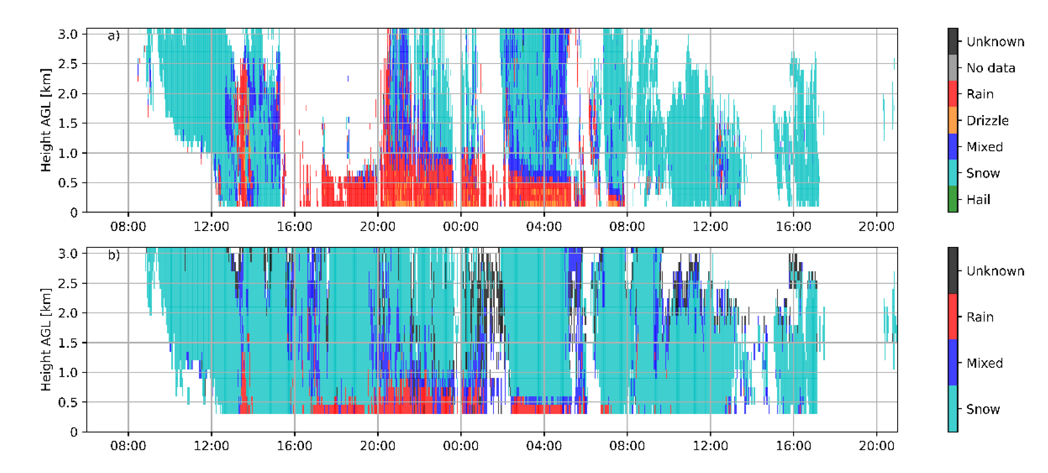
4.3. Precipitation Type
5. Discussion
6. Conclusions
Supplementary Materials
Author Contributions
Funding
Data Availability Statement
Acknowledgments
Conflicts of Interest
Appendix A


| Case | 5-min Interval of 1-min Types | Type Chosen | ||||
|---|---|---|---|---|---|---|
| m1 | m2 | m3 | m4 | m5 | ||
| 1 | Rain | Rain | Rain | Rain | Rain | Rain |
| 2 | Snow | Snow | Snow | Snow | Snow | Snow |
| 3 | Rain | Rain | Rain | Rain | Mixed | Rain |
| 4 | Snow | Snow | Snow | Snow | Mixed | Snow |
| 5 | Rain | Rain | NoPrec | Snow | Snow | Mixed |
| 6 | Rain | Rain | Rain | Snow | Snow | Mixed |
| 7 | Snow | Snow | Snow | Rain | Rain | Mixed |
| 8 | NoPrec | NoPrec | NoPrec | Rain | Rain | NoPrec |
| 9 | Rain | Rain | Rain | Rain | Snow | Mixed |
| 10 | Snow | Snow | Snow | Snow | Rain | Mixed |
| 11 | Rain | Rain | Rain | Mixed | Mixed | Mixed |
Appendix B
References
- Yamamoto, M. New Observations by Wind Profiling Radars. In Doppler Radar Observations—Weather Radar, Wind Profiler, Ionospheric Radar, and Other Advanced Applications; Bech, J., Chau, J., Eds.; InTech: London, UK, 2012; ISBN 978-953-51-0496-4. [Google Scholar]
- Lehmann, V.; Brown, W. Radar Wind Profiler. In Springer Handbook of Atmospheric Measurements; Foken, T., Ed.; Springer: Cham, Switzerland, 2021; pp. 901–933. ISBN 978-3-030-52171-4. [Google Scholar]
- Molod, A.; Salmun, H.; Dempsey, M. Estimating Planetary Boundary Layer Heights from NOAA Profiler Network Wind Profiler Data. J. Atmos. Ocean. Technol. 2015, 32, 1545–1561. [Google Scholar] [CrossRef]
- Nash, J.; Oakley, T.J. Development of COST 76 Wind Profiler Network in Europe. Phys. Chem. Earth Part B Hydrol. Ocean. Atmos. 2001, 26, 193–199. [Google Scholar] [CrossRef]
- Ishihara, M.; Kato, Y.; Abo, T.; Kobayashi, K.; Izumikawa, Y. Characteristics and Performance of the Operational Wind Profiler Network of the Japan Meteorological Agency. J. Meteorol. Soc. Jpn. Ser. II 2006, 84, 1085–1096. [Google Scholar] [CrossRef] [Green Version]
- Kim, K.-H.; Kim, M.-S.; Seo, S.-W.; Kim, P.-S.; Kang, D.-H.; Kwon, B.H. Quality Evaluation of Wind Vectors from UHF Wind Profiler Using Radiosonde Measurements. J. Environ. Sci. Int. 2015, 24, 133–150. [Google Scholar] [CrossRef] [Green Version]
- Liu, B.; Guo, J.; Gong, W.; Shi, L.; Zhang, Y.; Ma, Y. Characteristics and Performance of Wind Profiles as Observed by the Radar Wind Profiler Network of China. Atmos. Meas. Tech. 2020, 13, 4589–4600. [Google Scholar] [CrossRef]
- Gonzalez, S.; Bech, J.; Udina, M.; Codina, B.; Paci, A.; Trapero, L. Decoupling between Precipitation Processes and Mountain Wave Induced Circulations Observed with a Vertically Pointing K-Band Doppler Radar. Remote Sens. 2019, 11, 1034. [Google Scholar] [CrossRef] [Green Version]
- Zhang, Y.; Guo, J.; Yang, Y.; Wang, Y.; Yim, S. Vertical Wind Shear Modulates Particulate Matter Pollutions: A Perspective from Radar Wind Profiler Observations in Beijing, China. Remote Sens. 2020, 12, 546. [Google Scholar] [CrossRef] [Green Version]
- Garcia-Benadi, A.; Bech, J.; Gonzalez, S.; Udina, M.; Codina, B.; Georgis, J.F. Precipitation Type Classification of Micro Rain Radar Data Using an Improved Doppler Spectral Processing Methodology. Remote Sens. 2020, 12, 4113. [Google Scholar] [CrossRef]
- Wang, D.; Giangrande, S.E.; Feng, Z.; Hardin, J.C.; Prein, A.F. Updraft and Downdraft Core Size and Intensity as Revealed by Radar Wind Profilers: MCS Observations and Idealized Model Comparisons. J. Geophys. Res. Atmos. 2020, 125, e2019JD031774. [Google Scholar] [CrossRef]
- Politovich, M.K.; Goodrich, R.K.; Morse, C.S.; Yates, A.; Barron, R.; Cohn, S.A. The Juneau Terrain-Induced Turbulence Alert System. Bull. Am. Meteorol. Soc. 2011, 92, 299–313. [Google Scholar] [CrossRef]
- Udina, M.; Bech, J.; Gonzalez, S.; Soler, M.R.; Paci, A.; Miró, J.R.; Trapero, L.; Donier, J.M.; Douffet, T.; Codina, B.; et al. Multi-Sensor Observations of an Elevated Rotor during a Mountain Wave Event in the Eastern Pyrenees. Atmos. Res. 2020, 234, 104698. [Google Scholar] [CrossRef]
- Wang, C.; Chen, M.; Chen, Y. Impact of Combined Assimilation of Wind Profiler and Doppler Radar Data on a Convective-Scale Cycling Forecasting System. Mon. Weather Rev. 2022, 150, 431–450. [Google Scholar] [CrossRef]
- Degelia, S.K.; Wang, X.; Stensrud, D.J.; Turner, D.D. Systematic Evaluation of the Impact of Assimilating a Network of Ground-Based Remote Sensing Profilers for Forecasts of Nocturnal Convection Initiation during PECAN. Mon. Weather Rev. 2020, 148, 4703–4728. [Google Scholar] [CrossRef]
- Schraff, C.; Reich, H.; Rhodin, A.; Schomburg, A.; Stephan, K.; Periáñez, A.; Potthast, R. Kilometre-scale Ensemble Data Assimilation for the COSMO Model (KENDA). Q. J. R. Meteorol. Soc. 2016, 142, 1453–1472. [Google Scholar] [CrossRef]
- Liu, D.; Huang, C.; Feng, J. Influence of Assimilating Wind Profiling Radar Observations in Distinct Dynamic Instability Regions on the Analysis and Forecast of an Extreme Rainstorm Event in Southern China. Remote Sens. 2022, 14, 3478. [Google Scholar] [CrossRef]
- Ralph, F.M.; Neiman, P.J.; Ruffieux, D. Precipitation Identification from Radar Wind Profiler Spectral Moment Data: Vertical Velocity Histograms, Velocity Variance, and Signal Power–Vertical Velocity Correlations. J. Atmos. Ocean. Technol. 1996, 13, 545–559. [Google Scholar] [CrossRef]
- Radenz, M.; Bühl, J.; Lehmann, V.; Görsdorf, U.; Leinweber, R. Combining Cloud Radar and Radar Wind Profiler for a Value Added Estimate of Vertical Air Motion and Particle Terminal Velocity within Clouds. Atmos. Meas. Tech. 2018, 11, 5925–5940. [Google Scholar] [CrossRef] [Green Version]
- Tsai, S.-C.; Chu, Y.-H.; Chen, J.-S. Identification of Concurrent Clear-Air and Precipitation Doppler Profiles for VHF Radar and an Incorporating Study of Strongly Convective Precipitation with Dual-Polarized Microwave Radiometer. Atmosphere 2022, 13, 557. [Google Scholar] [CrossRef]
- Lundquist, J.D.; Neiman, P.J.; Martner, B.; White, A.B.; Gottas, D.J.; Ralph, F.M. Rain versus Snow in the Sierra Nevada, California: Comparing Doppler Profiling Radar and Surface Observations of Melting Level. J. Hydrometeorol. 2008, 9, 194–211. [Google Scholar] [CrossRef] [Green Version]
- Valdivia, J.M.; Scipión, D.E.; Milla, M.; Silva, Y. Multi-Instrument Rainfall-Rate Estimation in the Peruvian Central Andes. J. Atmos. Ocean. Technol. 2020, 37, 1811–1826. [Google Scholar] [CrossRef]
- Ryzhkov, A.V.; Schuur, T.J.; Burgess, D.W.; Heinselman, P.L.; Giangrande, S.E.; Zrnic, D.S. The Joint Polarization Experiment: Polarimetric Rainfall Measurements and Hydrometeor Classification. Bull. Am. Meteorol. Soc. 2005, 86, 809–824. [Google Scholar] [CrossRef] [Green Version]
- Besic, N.; Ventura, J.F.I.; Grazioli, J.; Gabella, M.; Germann, U.; Berne, A. Hydrometeor Classification through Statistical Clustering of Polarimetric Radar Measurements: A Semi-Supervised Approach. Atmos. Meas. Tech. 2016, 9, 4425–4445. [Google Scholar] [CrossRef] [Green Version]
- Chen, Y.; Liu, X.; Bi, K.; Zhao, D. Hydrometeor Classification of Winter Precipitation in Northern China Based on Multi-Platform Radar Observation System. Remote Sens. 2021, 13, 5070. [Google Scholar] [CrossRef]
- González, S.; Bech, J.; Garcia-Benadí, A.; Udina, M.; Codina, B.; Trapero, L.; Paci, A.; Georgis, J.-F. Vertical Structure and Microphysical Observations of Winter Precipitation in an Inner Valley during the Cerdanya-2017 Field Campaign. Atmos. Res. 2021, 264, 105826. [Google Scholar] [CrossRef]
- O’Hora, F.; Bech, J. Improving Weather Radar Observations Using Pulse-Compression Techniques. Meteorol. Appl. 2007, 14, 389–401. [Google Scholar] [CrossRef]
- Campistron, B.; Réchou, A. Rain Kinetic Energy Measurement with a UHF Wind Profiler: Application to Soil Erosion Survey of a Volcanic Tropical Island. In Proceedings of the 13th International Workshop on Technical and Scientific Aspects of MST Radars, Kühlungsborn, Germany, 19–23 March 2012; pp. 47–51. Available online: https://www.iap-kborn.de/MST13/files/mst13proceedings.pdf (accessed on 8 August 2022).
- Peters, G.; Fischer, B.; Andersson, T. Rain Observations with a Vertically Looking Micro Rain Radar (MRR). Boreal Environ. Res. 2002, 7, 353–362. [Google Scholar]
- Chang, W.Y.; Lee, G.W.; Jou, B.J.D.; Lee, W.C.; Lin, P.L.; Yu, C.K. Uncertainty in Measured Raindrop Size Distributions from Four Types of Collocated Instruments. Remote Sens. 2020, 12, 1167. [Google Scholar] [CrossRef] [Green Version]
- Tokay, A.; Wolff, D.B.; Petersen, W.A. Evaluation of the New Version of the Laser-Optical Disdrometer, OTT Parsivel2. J. Atmos. Ocean. Technol. 2014, 31, 1276–1288. [Google Scholar] [CrossRef]
- World Meteorological Organization. Manual on Codes—International Codes, Volume I.1, Annex II to the WMO Technical Regulations: Part A—Alphanumeric Codes; World Meteorological Organization: Geneva, Switzerland, 2019; ISBN 978-92-63-10306-2. [Google Scholar]
- Koistinen, J.; Saltikoff, E. Experience of Customer Products of Accumulated Snow, Sleet and Rain. COST75 Adv. Weather Radar Syst. 1998, 397, 406. [Google Scholar]
- Casellas, E.; Bech, J.; Veciana, R.; Pineda, N.; Miró, J.R.; Moré, J.; Rigo, T.; Sairouni, A. Nowcasting the Precipitation Phase Combining Weather Radar Data, Surface Observations, and NWP Model Forecasts. Q. J. R. Meteorol. Soc. 2021, 147, 3135–3153. [Google Scholar] [CrossRef]
- Casellas, E.; Bech, J.; Veciana, R.; Pineda, N.; Rigo, T.; Miró, J.R.; Sairouni, A. Surface Precipitation Phase Discrimination in Complex Terrain. J. Hydrol. 2021, 592, 125780. [Google Scholar] [CrossRef]
- Anandan, V.K.; Balamuralidhar, P.; Rao, P.B.; Jain, A.R.; Pan, C.J. An Adaptive Moments Estimation Technique Applied to MST Radar Echoes. J. Atmos. Ocean. Technol. 2005, 22, 396–408. [Google Scholar] [CrossRef]
- Allabakash, S.; Yasodha, P.; Bianco, L.; Reddy, S.V.; Srinivasulu, P. Improved Moments Estimation for VHF Active Phased Array Radar Using Fuzzy Logic Method. J. Atmos. Ocean. Technol. 2015, 32, 1004–1014. [Google Scholar] [CrossRef]
- Price-Whelan, A.M.; Sipőcz, B.M.; Günther, H.M.; Lim, P.L.; Crawford, S.M.; Conseil, S.; Shupe, D.L.; Craig, M.W.; Dencheva, N.; Ginsburg, A.; et al. The Astropy Project: Building an Open-Science Project and Status of the v2.0 Core Package. Astron. J. 2018, 156, 123. [Google Scholar] [CrossRef]
- Atlas, D.; Srivastava, R.C.; Sekhon, R.S. Doppler Radar Characteristics of Precipitation at Vertical Incidence. Rev. Geophys. 1973, 11, 1–35. [Google Scholar] [CrossRef]
- Ralph, F.M.; Neiman, P.J.; van de Kamp, D.W.; Law, D.C. Using Spectral Moment Data from NOAA’s 404-MHz Radar Wind Profilers to Observe Precipitation. Bull. Am. Meteorol. Soc. 1995, 76, 1717–1739. [Google Scholar] [CrossRef]
- Ulbrich, C.W. Natural Variations in the Analytical Form of the Raindrop Size Distribution. J. Clim. Appl. Meteorol. 1983, 22, 1764–1775. [Google Scholar] [CrossRef]
- Chu, Y.-H.; Su, C.-L. An Investigation of the Slope–Shape Relation for Gamma Raindrop Size Distribution. J. Appl. Meteorol. Climatol. 2008, 47, 2531–2544. [Google Scholar] [CrossRef]
- Gunn, R.; Kinzer, G.D. The Terminal Velocity of Fall for Water Droplets in Stagnant Air. J. Meteorol. 1949, 6, 243–248. [Google Scholar] [CrossRef]
- Cerro, C.; Bech, J.; Codina, B.; Lorente, J. Modeling Rain Erosivity Using Disdrometric Techniques. Soil Sci. Soc. Am. J. 1998, 62, 731–735. [Google Scholar] [CrossRef]
- Jolliffe, I.T.; Stephenson, D.B. Forecast Verification: A Practitioner’s Guide in Atmospheric Science; John Wiley & Sons: Hoboken, NJ, USA, 2012; ISBN 978-1-119-96000-3. [Google Scholar]


| Instrument (Institution) | Longitude (°) | Latitude (°) | Height ASL (m) |
|---|---|---|---|
| RWP (Météo-France) | 1.83759 E | 42.39688 N | 1079 |
| MRR2 (University of Barcelona) | 1.86650 E | 42.38643 N | 1099 |
| Disdrometer (University of Barcelona) | 1.86655 E | 42.38643 N | 1101 |
| AWS S0 (Meteorological Service of Catalonia) | 1.86640 E | 42.38605 N | 1097 |
| AWS S8 (Météo-France) | 1.82980 E | 42.39340 N | 1088 |
| Feature | RWP | MRR2 |
|---|---|---|
| Manufacturer, model | Degreane, PCL1300 | Metek, MRR2 |
| Frequency (GHz) | 1.247 | 24.23 |
| Radio band | UHF | K |
| Number of range gates | 45 | 32 |
| Number of Doppler bins | 128 | 64 |
| Peak power (W) | 2500 | 0.05 |
| Pulse width (µs) | 1 | --- |
| Maximum height (km) | 6.5 | 3.1 |
| Minimum reflectivity at 1 km (dBZ) | −15.0 | −4.7 |
| Approach | Type | Condition |
|---|---|---|
| A73 | Rain | |
| Mixed | and ≥ w ≥ | |
| Snow | ||
| Unknown | None of the above | |
| R95 | Rain | |
| Mixed | ||
| Snow | ||
| Unknown | None of the above |
| Disdrometer Precipitation Type | WMO Table 4677 Values | Method2 Precipitation Type |
|---|---|---|
| Drizzle | From 51 to 53 | Rain |
| Drizzle with rain | From 58 to 59 | |
| Rain | From 61 to 65 | |
| Rain, drizzle with snow | From 68 to 69 | Mixed |
| Snow | From 71 to 75 | Snow |
| Snow grains | 77 | |
| Soft hail | From 87 to 88 | |
| Hail | From 89 to 90 | Unknown |
| Precipitation Type | Method2 with A73 | Method2 with R95 | Disdrometer |
|---|---|---|---|
| Rain | 113 | 124 | 158 |
| Mixed | 46 | 60 | 37 |
| Snow | 118 | 109 | 85 |
| Unknown | 5 | 2 | - |
| Total | 282 | 295 | 280 |
| Approach | Parameter | Time Interval (min) | POD (1) | FAR (0) | ORSS (1) | TSS (1) |
|---|---|---|---|---|---|---|
| A73 | Rain | 0 | 0.78 | 0.10 | 0.94 | 0.68 |
| Mixed | 0.19 | 0.81 | 0.41 | 0.10 | ||
| Snow | 0.90 | 0.40 | 0.93 | 0.66 | ||
| No Precipitation | 0.91 | 0.08 | 0.98 | 0.83 | ||
| Rain | 5 | 0.79 | 0.10 | 0.95 | 0.70 | |
| Mixed | 0.24 | 0.76 | 0.57 | 0.16 | ||
| Snow | 0.92 | 0.35 | 0.95 | 0.68 | ||
| No Precipitation | 0.92 | 0.08 | 0.98 | 0.84 | ||
| Rain | 10 | 0.79 | 0.10 | 0.95 | 0.69 | |
| Mixed | 0.31 | 0.69 | 0.68 | 0.23 | ||
| Snow | 0.93 | 0.32 | 0.95 | 0.97 | ||
| No Precipitation | 0.92 | 0.08 | 0.98 | 0.84 | ||
| R95 | Rain | 0 | 0.88 | 0.05 | 0.99 | 0.83 |
| Mixed | 0.33 | 0.78 | 0.57 | 0.21 | ||
| Snow | 0.77 | 0.44 | 0.83 | 0.54 | ||
| No Precipitation | 0.88 | 0.07 | 0.98 | 0.81 | ||
| Rain | 5 | 0.88 | 0.05 | 0.99 | 0.84 | |
| Mixed | 0.55 | 0.52 | 0.81 | 0.44 | ||
| Snow | 0.82 | 0.37 | 0.88 | 0.60 | ||
| No Precipitation | 0.89 | 0.07 | 0.98 | 0.82 | ||
| Rain | 10 | 0.89 | 0.05 | 0.99 | 0.84 | |
| Mixed | 0.59 | 0.55 | 0.84 | 0.48 | ||
| Snow | 0.83 | 0.34 | 0.90 | 0.62 | ||
| No Precipitation | 0.89 | 0.07 | 0.98 | 0.82 |
Publisher’s Note: MDPI stays neutral with regard to jurisdictional claims in published maps and institutional affiliations. |
© 2022 by the authors. Licensee MDPI, Basel, Switzerland. This article is an open access article distributed under the terms and conditions of the Creative Commons Attribution (CC BY) license (https://creativecommons.org/licenses/by/4.0/).
Share and Cite
Garcia-Benadi, A.; Bech, J.; Udina, M.; Campistron, B.; Paci, A. Multiple Characteristics of Precipitation Inferred from Wind Profiler Radar Doppler Spectra. Remote Sens. 2022, 14, 5023. https://0-doi-org.brum.beds.ac.uk/10.3390/rs14195023
Garcia-Benadi A, Bech J, Udina M, Campistron B, Paci A. Multiple Characteristics of Precipitation Inferred from Wind Profiler Radar Doppler Spectra. Remote Sensing. 2022; 14(19):5023. https://0-doi-org.brum.beds.ac.uk/10.3390/rs14195023
Chicago/Turabian StyleGarcia-Benadi, Albert, Joan Bech, Mireia Udina, Bernard Campistron, and Alexandre Paci. 2022. "Multiple Characteristics of Precipitation Inferred from Wind Profiler Radar Doppler Spectra" Remote Sensing 14, no. 19: 5023. https://0-doi-org.brum.beds.ac.uk/10.3390/rs14195023