Inverted Algorithm of Groundwater Storage Anomalies by Combining the GNSS, GRACE/GRACE-FO, and GLDAS: A Case Study in the North China Plain

Abstract

As the largest groundwater drainage region in China, the per capita water resources in the North China Plain (NCP) account for only one-seventh of the country’s available water resources. Currently, the NCP is experiencing a serious water shortage due to the overexploitation of groundwater resources and a subsequent series of natural disasters. Thus, accurate regional assessments and effective water resource management policies are of critical importance. To accomplish this phenomenon, the daily terrestrial water storage anomaly (TWSA) over the NCP is calculated from the combination of the GNSS vertical deformation sequences (seasonal items) and GRACE (trend items). The groundwater storage anomaly (GWSA) in the NCP is obtained by subtracting the canopy water, soil water, and snow water equivalent components from the TWSA. The inversion results of this study are verified by comparisons with the Global Land Data Assimilation System (GLDAS) data products. The elevated annual amplitude areas are located in Beijing and Tianjin, and the Pearson correlation coefficient (PCC), root mean square error (RMSE), and Nash–Sutcliffe efficiency (NSE) between the two GWSA results are 0.67, 4.01 cm, and 0.61, respectively. This indicates that the methods proposed in this study are reliable. Finally, the groundwater drought index was calculated for the period from 2011 to 2021, and the results showed that 2019 was the driest year, with a drought severity index value of −0.12, indicative of slightly moderate drought conditions. By calculating and analyzing the annual GWSA, this work shows that the South–North Water Transfer Project does provide some regional drought mitigation.

1. Introduction

Groundwater is an important resource for urban construction, agricultural production, and residential life, which plays a pivotal role in the development of China’s national economy [1]. With the process of urbanization accelerating and the improvements in industrialization, the issue of groundwater overdraft has become increasingly serious in recent years [2]. This is especially true in the North China Plain (NCP), where the massive exploitation of groundwater resources has triggered a series of natural disasters, such as drought, surface subsidence, and soil erosion, which have severely impacted the economic stability and development of the NCP [3]. Therefore, an appropriate monitoring of groundwater storage is critical for a macroscopic analysis of the groundwater resources spatial distribution [4]. Traditional groundwater observation methods mainly monitored the water level, water quality, soil moisture, and other parameters via observation wells or monitoring stations. However, the laborious process of station and well construction consumes a great deal of human and material resources [5]. Although groundwater wells can accurately monitor the change of groundwater level over local regions, the uneven distribution of these wells greatly limits the monitoring of groundwater changes over large-scale regions. Meanwhile, the construction of groundwater wells consumes a lot of manpower and material resources. Therefore, it is meaningful to find an alternative strategy to accurately monitor the groundwater level changes in the large-scale regions.

In 2002, the successful launch of the Gravity Recovery and Climate Experiment (GRACE) satellites provided an unprecedented opportunity to monitor groundwater storage anomalies (GWSA) [6,7,8,9,10]. As a result, a large number of studies have since been carried out around the world, such as in Cambodia [11], California [12,13], Northern China [14], the NCP [15], and Guanzhong region [16]. Monitored data of GRACE satellites can accurately depict regional load changes based on the inversion of local gravity anomalies [17]. However, due to the GRACE satellites’ aging power supply system, it was not possible to accurately reflect gravity anomalies, and the mission was ended in 2017. The GRACE satellites’ next-generation successor, GRACE Follow-On (GRACE-FO), was launched in 2018, with a gap of nearly one year between the two missions [8,18,19]. Meanwhile, due to the inherent characteristics of GRACE satellites, inversion results from GRACE data have coarser spatial and temporal resolutions, usually 1° × 1° (spatial) and one month (temporal), respectively [20,21]. As a result, the GWSA in local areas cannot be monitored in real time using GRACE gravity satellites [21,22]. Therefore, finding an alternative means to effectively monitor GWSA with high spatiotemporal resolution is critical.

The seasonal migration of large-scale water masses causes not only changes in regional gravity but also vertical deformation of the Earth’s crust due to subsidence or uplift; this process is called crustal nontectonic deformation [23,24,25,26]. The factors affecting crustal nontectonic deformation include atmospheric load, terrestrial water storage, ocean load disturbance, and human activities [27,28]. Among them, the change in terrestrial water storage is the most important factor influencing the deformation, and this relationship can be established by combining Green’s load function and the crustal load model [29,30,31]. In recent years, the global navigation satellite system (GNSS) observation tools and computational strategies have become more sophisticated. This phenomenon is beneficial to the wide application of GNSS-observed datasets [32]. Meanwhile, the Crustal Movement Observation Network of China (CMONOC) project was started in 1997 and can accurately and continuously monitor the vertical deformation of the Earth’s crust [33,34,35,36]. Numerous scholars have utilized the GNSS data provided by CMONOC to monitor crustal vertical deformation and study geophysical phenomena in typical regions of China, such as Southwest China [37], Sichuan Province [38], the NCP [15,39], Qinghai–Tibet Plateau [40,41,42], etc. Therefore, the GNSS deformation sequence products provided by CMONOC can be used to accurately analyze crustal deformation characteristics and identify water storage anomalies with high spatial and temporal resolution to compensate for the limitations of the GRACE/GRACE-FO dataset.

This study applies the GNSS and GRACE/GRACE-FO to derive the terrestrial water storage anomalies (TWSA). Then, the components (canopy water, snow water, and soil water) of the Global Land Data Assimilation System (GLDAS) are deducted from TWSA to obtain the GWSA over the NCP region between 2010 and 2021. The following sections are organized as follows. Section 2 introduces the data and methods applied in this study. Section 3 summarizes the experimental results of this study, including the inversion of the TWSA, GWSA results, and the validation of the GWSA inversion results. Section 4 calculates and discusses the drought severity index (DSI) over the NCP. Meanwhile, this section discusses the effects of the South–North Water Diversion Project. Section 5 summarizes the results of this study.

2. Materials and Methods

2.1. The Study Area

The North China Plain (NCP), located between 32°N and 40°N latitude and from 114°E to 121°E longitude, is the most populous of the three major Chinese plains and is a major component of China’s eastern plain [43]. The NCP reaches the southern foot of Yanshan Mountain in the north, the northern side of Dabie Mountain in the south, Taihang Mountains and Fuyu Mountains in the west, and the Bohai Sea and Yellow Sea in the east. The total area of the NCP is approximately 300,000 square kilometers and accounts for 3.1% of the total land area of China. The total population is 339 million, accounting for 24.2% of the total population of China. However, the spatial distribution of water resources over the NCP is extremely uneven, and natural disasters such as droughts and floods are frequent occurrences. These conditions adversely impact the economic development of the NCP. To alleviate water shortage in North China, the South–North Water Transfer Project was implemented in 2002. This project contains three lines (i.e., east, central, and west). The central line of this project officially began delivering water to North China (including Beijing, Tianjin, Hebei, and Henan Province) in December 2014, supplying 950 million km³ of water resources per year from the Danjiangkou Reservoir to the north of China. The east line of this project will gradually expand the scale of water transfer and extend the water transmission line by using the existing river for the north water transfer project in Jiangsu Province, which aims to solve the water shortage problems in the east of the Huang-Huaihai Plain. The western line of this project builts dams and reservoirs in the upper reaches of the Yangtze River, Tongtian River, Yalong River, and Dadu River. The water-receiving areas of the west line mainly include Qinghai, Gansu, Ningxia, Inner Mongolia, Shaanxi, and Shanxi [44,45].

2.2. Data

2.2.1. GNSS Data

In this study, we employed the observation data from 26 GNSS stations located on bedrock, which were provided by the CMONOC [46]. The software of GNSS at MIT/Global Kalman filter (GAMIT/GLOBK) (http://geoweb.mit.edu/gg/) (accessed on 2 November 2022) was utilized to calculate the GNSS sequences, and the solution parameters are shown in Table 1 [47]. However, due to the influence of factors such as earthquakes and antenna replacement, there are clear disruptions in the step signal and anomalies in GNSS sequences [48]. Thus, GNSS values that exceeded three standard deviations were removed from this study, and the step signal was corrected to obtain a more accurate GNSS site deformation sequence. The spatial distribution of GNSS stations in and around the NCP region is shown in Figure 1.

2.2.2. GRACE Mascon Dataset

Regional terrestrial water storage variability can be effectively obtained through inversion of the GRACE and GRACE-FO time-varying gravity fields by using the following equation [49,50]:

$$\Delta h(\theta ,\phi )=\frac{A{\rho }_e\pi }{3{\rho }_w}\times {\displaystyle \sum _{l=0}^{\infty }{\displaystyle \sum _{m=0}^l\frac{2h_l+1}{1+k_l}}}\times W_l\times {\overline{P}}_{l,m}(\cos \theta )\times [\Delta C_{lm}\cos (m\phi )+\Delta S_{lm}\sin (m\phi )]$$

(1)

where $\Delta h$ denotes the equivalent water height of the TWSA, A denotes the radius of the Earth (6371.39 km), ${\rho }_e$ denotes the mean density of the Earth (5.51 × 10³ kg/m³), ${\rho }_w$ denotes the density of water (10³ kg/m³), $h_l$ and $k_l$ denote the load Love numbers of order l [51], W_l denotes the kernel function of Gaussian filter, ${\overline{P}}_{l,m}$ denotes the fully specified connective Legendre function, and $\Delta C_{lm}$ and $\Delta S_{lm}$ denote the amount of variation within the spherical harmonic coefficients of the Earth’s gravity field obtained from GRACE/GRACE-FO global geopotential models (GGMs) (http://icgem.gfz-potsdam.de/series) (accessed on 2 November 2022).

This paper used GRACE mass concentration (mascon) datasets from the Center for Space Research (CSR) and Jet Propulsion Laboratory (JPL) for the period from 2011 to 2021 [52,53]. Then, the TWSA sequences of the NCP region were extracted by the boundary file. To minimize the solution uncertainty of the data products in this study, the average of the two datasets was taken as the final TWSA of GRACE/GRACE-FO. Furthermore, we also utilized the method of cubic spline interpolation to transform the GRACE/GRACE-FO datasets into daily:

$$\Delta TWS{A}_{\mathrm{GRACE}}=\frac{\Delta Masco{n}_{CSR}+\Delta Masco{n}_{JPL}}{2}$$

(2)

where $\Delta Masco{n}_{CSR}$ denotes the TWSA result by CSR and the $\Delta Masco{n}_{JPL}$ denotes the TWSA result by JPL.

2.2.3. GLDAS Dataset

To derive the GWSA over the NCP, this study utilized datasets from the GLDAS Noah hydrological model at 3 h temporal resolution and daily-resolved data from GLDAS V2.2. The daily-resolved GLDAS V2.2 dataset begins on 1 February 2003 and extends to the present and has a spatial resolution of 0.25° × 0.25°. Twenty-six variables are included in the GLDAS V2.2 dataset, including terrestrial water storage, groundwater storage, canopy water, snow depth equivalent, evapotranspiration, rainfall rate, and snowfall rate [54]. In this study, terrestrial water storage, groundwater storage, and canopy water over the NCP were selected from the GLDAS V2.2 dataset for the period from 2011 to 2022. However, to accurately calculate the anomalous changes in groundwater storage in the NCP, snow water and soil water also needed to be deducted from terrestrial water storage. Therefore, the 3-hourly resolved GLDAS Noah model was also used in this study, which contains 40 variables, including soil water data (0~10 cm, 10~40 cm, 40~100 cm, and 100~200 cm), snow depth equivalent, and average surface temperature. The snow depth equivalent and soil water data at each depth were used from the GLDAS Noah model. To maintain a consistent spatial and temporal resolution, the extracted 3 h snow depth equivalent and total soil water data were averaged to generate datasets at the appropriate resolution. The extraction and preprocessing of the variables in the GLDAS dataset provided a robust database for the NCP groundwater storage inversion [54,55].

2.3. Method

2.3.1. Crustal Load Inversion Theory

The Earth is an elastic sphere, and when the load on the Earth’s surface (e.g., surface water, snow, ice, etc.) changes, the crust deforms accordingly. This deformation is known as load deformation [56]. Fortunately, the Green’s function can be used to establish the relationship between the load mass and deformation [57]. The crustal load deformation mainly manifests in the horizontal and vertical directions. However, crustal load deformation is more pronounced in the vertical direction where the load-deformation amplitude is approximately 2~3 times that in the horizontal direction [58,59]. Green’s function describes the crustal vertical load-deformation as follows [60]:

$$U_{green}={\displaystyle \sum _{n=0}^{\infty }{h}_n{\Gamma }_n}\frac{4\pi GR}{g(2n+1)}{P}_n(\cos \theta )$$

(3)

where $\theta$ denotes the angular radius from the center of the deformation, $P_n$ denotes the Legendre polynomial, G denotes Newton’s universal gravitational constant, R denotes the radius of the Earth, h_n denotes the loading Love number, and g denotes the acceleration of gravity. The derivation of the ${\Gamma }_n$ function is as follows [60]:

$${\Gamma }_n=\frac{1}{2}\left[P_{n-1}(\cos \theta )-P_{n+1}(\cos \theta )\right],(n>0)$$

(4)

where $\theta$ denotes the angular radius from the center of the deformation and P denotes the Legendre polynomial. When n equals 0, the expression of the $\Gamma$ function is as follows [60]:

$${\Gamma }_0=\frac{1}{2}(1-\cos \theta )$$

(5)

First, this study used the corrected GNSS vertical deformation series as the database to estimate the water storage variability at a 0.25° × 0.25° spatial scale. Then, the solutions were regularized using the curvature smoothing algorithm and were appended to the solution matrix as a set of constraints [61]. Specifically, for each time period within this study, the suppressed least squares problem was minimized to estimate the daily TWSA.

$${\mathrm{Load}}_{\mathrm{TWSA}}={((Gx-b)/\sigma )}^2+{\beta }^2{(L(x))}^2\to \min$$

(6)

where G denotes the Green’s function coefficient matrix, $\sigma$ denotes the standard deviation of the GNSS vertical displacement series, b denotes the observed sequence of deformation of the grid and the corrected GNSS vertical deformation series, L denotes the Laplace operator, and $\beta$ denotes the smoothing factor. Therefore, the change of TWSA can be obtained by the cubic spline interpolation.

2.3.2. Groundwater Storage Estimation

TWSA mainly includes GWSA, soil water changes, surface water anomaly changes, snow water equivalent changes, and biological water quality changes. The effect of biologically induced changes to water quality on terrestrial water storage variability is extremely small and can be ignored [62]. Therefore, the groundwater storage changes can be obtained according to the following equation:

$$GWSA=TWSA-W_{Can}-W_{soil}-W_{snow}$$

(7)

where GWSA indicates the groundwater storage anomaly, TWSA indicates the terrestrial water storage anomaly, W_can indicates the canopy water change, W_soil indicates the total soil water change from 0 to 200 mm—which includes four layers of data from 0 to 10 cm, 10 to 40 cm, 40 to 100 cm, and 100 to 200 cm—and W_snow indicates the snow water equivalent.

2.3.3. Groundwater Drought Index

In this study, the groundwater drought index calculation method, as proposed by Han et al. [63], was used to investigate the groundwater drought conditions over the NCP. The value of DSI can be calculated by the following equation:

$$DS{I}_{i,j}=\frac{GWS{A}_{i,j}-\overline{GWS{A}_j}}{{\sigma }_j}$$

(8)

where i and j denote the number of years and months, respectively, DSI denotes the groundwater drought index of the study area, GWSA_i,j denotes the groundwater storage anomaly change in month j of year i, and $\overline{GWS{A}_j}$ and ${\sigma }_j$ denote the mean and standard deviation of GWSA, respectively. The classification of groundwater drought classes derived from DSI is shown in Table 1.

Table 1. DSI values and the corresponding groundwater drought classification [63].

Grade	Classification	DSI Value
L1	No drought	−0.8 < DSI
L2	Mild drought	−1.3 < DSI ≤ −0.8
L3	Moderate drought	−1.60 < DSI ≤ −1.30
L4	Severe drought	−2.00 < DSI ≤ −1.60
L5	Extreme drought	DSI ≤ −2.00

Table 1. DSI values and the corresponding groundwater drought classification [63].

Grade	Classification	DSI Value
L1	No drought	−0.8 < DSI
L2	Mild drought	−1.3 < DSI ≤ −0.8
L3	Moderate drought	−1.60 < DSI ≤ −1.30
L4	Severe drought	−2.00 < DSI ≤ −1.60
L5	Extreme drought	DSI ≤ −2.00

2.3.4. Evaluation Index

In this study, we utilized the root mean squared error (RMSE) [64], Pearson’s correlation coefficient (PCC) [28], and Nash–Sutcliffe efficiency coefficient (NSE) [65]. The accuracy of the inversion results was evaluated by these three metrics, which are calculated as follows:

$$RMSE=\sqrt{\frac{1}{n}{\displaystyle \sum _{i=1}^n{\left(Y_i-X_i\right)}^2}}$$

(9)

$$NSE=1-\frac{{\displaystyle {\sum }_{i=1}^n{\left(Y_i-X_i\right)}^2}}{{\displaystyle {\sum }_{i=1}^n{\left(X_i-\overline{X}\right)}^2}}$$

(10)

$$PCC=\frac{{\displaystyle {\sum }_{i=1}^n\left(X_i-\overline{X}\right)\left(Y_i-\overline{Y}\right)}}{\sqrt{{\displaystyle {\sum }_{i=1}^n{\left(X_i-\overline{X}\right)}^2}}\sqrt{{\displaystyle {\sum }_{i=1}^n{\left(Y_i-\overline{Y}\right)}^2}}}$$

(11)

where Y represents the true series, X represents the inversion result, $\overline{Y}$ and $\overline{X}$ represent the mean values of Y and X, respectively, and n represents the number of discrete points in the sequences. The RMSE can be used to evaluate the deviation of dispersion between the inversion result and the actual value; the smaller the RMSE value is, the more accurate the results of the inversion. The NSE is mainly used to evaluate the quality of the hydrological model, and its value is less than or equal to 1; the larger the value is, the better the hydrological model is. When NSE is close to 0, it indicates that the hydrological model effect is close to the average level of the observed values. The PCC is mainly used to describe the linear correlation between two series. The PCC value ranges between −1 and 1. The closer the value is to 1, the more reliable the inversion result is.

The method impalement in this study primarily consisted of the following three modules: Module 1 mainly preprocessed the observed GNSS data and obtained the hydrological load deformation series by deducting the atmospheric loading and nonmarine tidal loading. Then, this module derived the seasonal variability of the TWSA in the NCP by combining Green’s load function and the crustal load model. Module 2 extracted the TWSA variability in the NCP using the equivalent water height variables provided by the GRACE Mascon. Meanwhile, the module extracted the trend term of TWSA using the new correlation variational mode decomposition (CVMD) algorithm and added this trend term to the TWSA results of GNSS. Module 3 calculated and analyzed the characteristics of the GWSA over the NCP. Finally, this module analyzed the impact of the South–North Water Transfer Project on groundwater storage. The main flow chart of this study is shown in Figure 2.

3. Results

3.1. Inversion of TWSA Seasonal Features Based on GNSS

The GAMIT/GLOBK software was used to process the raw observation data and obtain the GNSS station coordinate sequences (the solution strategy is shown in

Table 2. Table of GNSS data resolution strategies [66].

Parameters	Value	Parameters	Value
Reference frame	ITRF a 2008	Flat Difference	Weighted least squares estimation + Kalman filtering
Height cutoff angle	10°	Ionosphere	LC b portfolio observations
A priori troposphere	0.5 m	Earth’s rotation parameters	Polar shift, UT1 c
Mapping functions	HGMF d, DGMF e	Inertial coordinate system	J2000.0
Satellite phase center	IGS f ANTEX g Model	Phase movement	IAU h 1980

^a ITRF: International Terrestrial Reference Frame, ^b LC: linear combination, ^c UT: universal time, ^d HGMF: humid global mapping function, ^e DGMF: dry global mapping function, ^f International GNSS Service for Geodynamics, ^g ANTEX: antenna exchange, ^h IAU: International Astronomical Union.

). Since the vertical amplitude of crustal load deformation is much larger than the amplitude in the horizontal direction, the GNSS vertical deformation sequence was applied as the initial signal in this study. Due to the effects of earthquake and antenna replacement, there are step issues and outliers in the original GNSS vertical deformation sequence. To resolve this problem, the step terms were corrected and outliers that were larger than three times the median error of the sequence were removed. Additionally, vertical crustal deformation mainly consists of tectonic deformation driven by the Earth’s internal forces and nontectonic deformation driven by the Earth’s external force. Nontectonic deformation of the Earth’s crust is mainly driven by hydrological, atmospheric, and tidal factors. The GNSS observatory monitors all crustal deformation, so the GNSS vertical deformation series are detrended, and the preprocessed crustal vertical deformation series are corrected with non-oceanic atmospheric corrections and non-oceanic tidal corrections using the non-tidal atmospheric loading (NATL) and non-tidal ocean loading (NOTL) models. Thus, the hydrological load deformation sequences were obtained and the TWSA in NCP was inverted by using the Green’s function. The daily TWSA inversion results based on GNSS and the TWSA fit outcomes by CVMD are shown in Figure 3.

From Figure 3, it can be seen that there are obvious annual and semiannual TWSA characteristics as derived from the GNSS inversion. Since the South–North Water Transfer Project was officially completed in December 2014, the whole study period was divided into two periods, 2011~2014 and 2015~2022. It can be seen from Figure 3a that the TWSA amplitude after 2015 is significantly higher than that of 2011~2014, which is consistent with the timing of the South–North Water Transfer Project. Moreover, the annual characteristics of the TWSA in the NCP are more obvious than the semiannual characteristics, with a maximum annual amplitude of 170 mm, while the semiannual amplitude is only 27 mm. For the semiannual amplitude, the peak areas are evidently located in the Beijing and Tianjin regions. However, due to the limitation of GNSS inversion, only the periodicity of the TWSA sequence can be detected. In addition, the trend term is especially important for the effective management of water resources. Therefore, this study included the TWSA obtained from GNSS inversion based on the GRACE/GRACE-FO Mascon dataset for the purpose of more accurate monitoring of regional TWSA.

3.2. TWSA Trend-Feature Extraction Based on GRACE/GRACE-FO

Since the TWSA obtained from GNSS inversion only include the seasonal terms and phases of the TWSA signals, GRACE/GRACE-FO mascon data were combined with GNSS results to derive TWSA trends. To better superimpose the GNSS inversion results on trend terms obtained from GRACE/GRACE-FO solutions, both GNSS inversion results and GRACE/GRACE-FO results were corrected with first-order items. The correction of the first-order items was to deduct the first value of the sequence. Additionally, to calculate the reliability of the TWSA results obtained from this method, GLDAS V2.2 TWSA data were used as the validation data. The comparison results are shown in Figure 4.

Figure 4a shows that the seasonal and trend terms of the TWSA can be effectively inferred based on the inversion methods applied in this study. Furthermore, the annual amplitude of TWSA from the GLDAS dataset shows a decreasing trend from west to east, and there is a funnel region over Beijing (Figure 4b), which shows the color of dark red. This phenomenon may be caused by the large demand for water in Beijing. The trend term of the TWSA results shows an increase from north to south, but the spatial resolution of the TWSA in this study is coarse due to the low spatial resolution of the GRACE/GRACE-FO dataset. However, the consistency of the sequence trend performance is better, and the TWSA results derived by this inversion method are more consistent than those of the GLDAS dataset and have a PCC value of 0.72 and an RMSE of 2.8 cm between the two sequences. In summary, the TWSA in the NCP region can be accurately derived by using the method of this study, which provides a large database for the calculation of GWSA.

3.3. Inversion and Validation of GWSA

In this study, the GWSA over the NCP region was calculated based on the TWSA derived by GNSS and GRACE/GRACE-FO, the canopy water data in the GLDAS V2.2 dataset, and the snow water equivalent and 0~200 mm soil water data in the GLDAS Noah dataset. To ensure the uniformity of the data, the first-order term correction process was applied to each variable in this experiment. The results of the inversion are shown in Figure 5.

As shown in Figure 5, the GWSA sequence characteristics and annual variation characteristics of the NCP can be calculated based on the inversion strategy of this study. Figure 5b represents the spatial characteristics of the annual amplitude of the GWSA, which was obtained based on the calculation of the longitudinal data of each grid in Figure 5a. In addition, its annual amplitude has obvious peaks in the western part of the NCP (Shijiazhuang) and the Tianjin region, which is consistent with the previous calculation [67]. Figure 5c shows that the groundwater storage in the NCP is decreasing overall. In addition, the annual amplitude after the completion of the South–North Water Transfer Project (gray shaded area) is significantly higher than before the South–North Water Transfer Project (white area). To verify the reliability of the inversion results of this study, the experimental results were compared with the GWSA variables of the GLDAS V2.2, and the comparison results are shown in Figure 6.

Figure 6 represents the comparative results of the GWSA in the NCP calculated on the basis of the inversion method presented in this study. According to Figure 6d, the overall sequence performance of this result is better than that of GLDAS, with PCC, RMSE, and NSE values of 0.69, 4.01 cm, and 0.61, respectively. Moreover, the slope of the sequence calculated in this study (−8.52 mm/y) is closer to that of the previous study [67]. Figure 6a,b represent the spatial distribution of the annual amplitudes and trends of GWSA in the GLDAS dataset, respectively. By comparing Figure 5b and Figure 6a, it can be seen that the raised areas of the annual amplitudes are all located in Tianjin, Shijiazhuang, and the southern part of the NCP. However, the annual amplitudes based on the GNSS and GRACE inversions are slightly larger than those of the GLDAS dataset, because the GNSS observations reflect the overall crustal vertical deformation, which bias the results, and only the nonmarine tidal and nonmarine atmospheric corrections were removed in this study. By comparing Figure 6b,c, we can see that the lowest area of GLDAS and the inversion results of this study are located in the central part of the NCP, while the trend-term peak areas are located in the northern and southern parts of the NCP. Meanwhile, the power spectrum of the GWSA results (this study and GLDAS) are plotted in Figure 6e. It can be seen from Figure 6e that the inversion results of this study are consistent with the sequence power amplitude of GLDAS in low frequency and intermediate frequency. Due to the existence of noise in the GNSS sequences, the amplitude of GWSA in the high-frequency part of the inversion results in this study is slightly higher than that of GLDAS. This further verifies the reliability of this inversion method to calculate GWSA in the region.

4. Discussion

4.1. Analysis of Groundwater Drought Characteristics in the NCP

As the political, economic, and agricultural center of China, the NCP accounts for 30% of the country’s groundwater consumption. Due to the geographical characteristics of the NCP, surface water reserves are low, and its freshwater resources are mainly distributed in groundwater. Nearly 60% of the freshwater resources in Henan Province and Beijing come from groundwater, with groundwater comprising more than 79% of the water supply sources in Hebei Province. In recent years, due to the development of industry and agriculture, groundwater reserves in the NCP have been heavily exploited. Groundwater drought occurs regularly in some regions owing to groundwater shortages. This issue seriously affects the economic development and stability of the NCP region. Therefore, it is necessary to monitor the terrestrial water variations and drought characteristics of the NCP. In the last two decades, scholars have also carried out a lot of research, which has made great contributions [67,68,69,70]. This section utilizes the GWSA results obtained in this study and combines with the groundwater drought index calculation method (Equation (8)) to calculate the groundwater drought situation over the NCP [63]. The groundwater drought indices are calculated from 2011 to 2021, and the results are shown in Figure 7.

As shown in Figure 7, mild drought conditions are prevalent from 2012 to 2013 and 2017 to 2019. The most obvious drought occurred in 2019, and with a DSI value of −0.12, the conditions were close to moderate drought. The DSI value reached −0.81 in 2017, which is indicative of mild drought. In terms of spatial distribution, the analysis shows that the southern part of the NCP is drier than the northern part (Figure 7a,b,e). The southern part of the NCP suffered from strong convective storms and floods in 2016, and its groundwater drought index slightly increased; however, a local drought occurred in the Beijing–Tianjin region. The groundwater drought situation in the NCP from 2020 to 2021 decreased compared with that in 2019, and its DSI showed a positive trend. This phenomenon is mainly due to the northward shift of the main precipitation region in China after 2019, which greatly has alleviated the drought problem in the NCP.

4.2. Impact of the South–North Water Diversion Project on GWSA

To alleviate the water shortage in the NCP, China implemented the South–North Water Transfer Project, the largest water transfer project in the world, to transfer water resources from the Yangtze River to the NCP. Construction of the project was officially completed at the end of 2014 and greatly improved the water supply and security of the water-scarce areas along the project route. Therefore, it is of great interest to analyze the extent to which the project affected the groundwater storage in the NCP region [71]. In this subsection, the spatial and temporal changes in groundwater storage are calculated for each year between 2011 and 2021. To facilitate the comparison of the amplitude differences between years, the annual GWSA series are corrected by their first-order terms. These results are shown in Figure 8.

Figure 8 shows that the opening of the South–North Water transfer project significantly improved the groundwater within the NCP. The spatial distribution shows a gradual GWSA decrease from south to north, though there are clear amplitude changes within Tianjin and Hebei Province (Figure 8e–i). The annual amplitude of the GWSA after the south-to-north transfer began (Figure 8e–k) is significantly higher than that before the south-to-north water transfer (Figure 8a–d), as shown in the sequence diagram. The amplitude of the GWSA sequence increased considerably after 2015, yet it still showed a downward trend (Figure 6d). This is due to the more urgent demand for groundwater from agriculture and industry after the South–North Water Transfer Project was completed in 2014 and indicates that groundwater overextraction is becoming a more serious problem. The spatial distribution of GWSA is most prominent in the NCP from 2017 to 2019 (Figure 8g–i), the GWSA amplitude is significantly higher than that in other years, and these issues persisted until 2020. In summary, the South–North Water Transfer Project does provide some drought mitigation for GWSA over the NCP.

5. Conclusions

Due to the complexity of GNSS deformation sequence composition, only the seasonal items of TWSA can be derived, which greatly limits the application of GNSS inversions in studying TWSA and GWSA. In this study, the GWSA of the NCP was obtained from the GNSS vertical deformation sequences, GRACE/GRACE-FO datasets, and the GLDAS data. The details are summarized as follows:

(1)

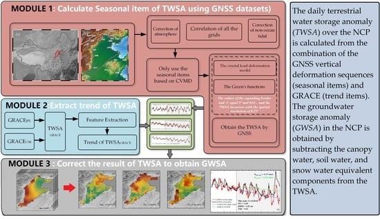
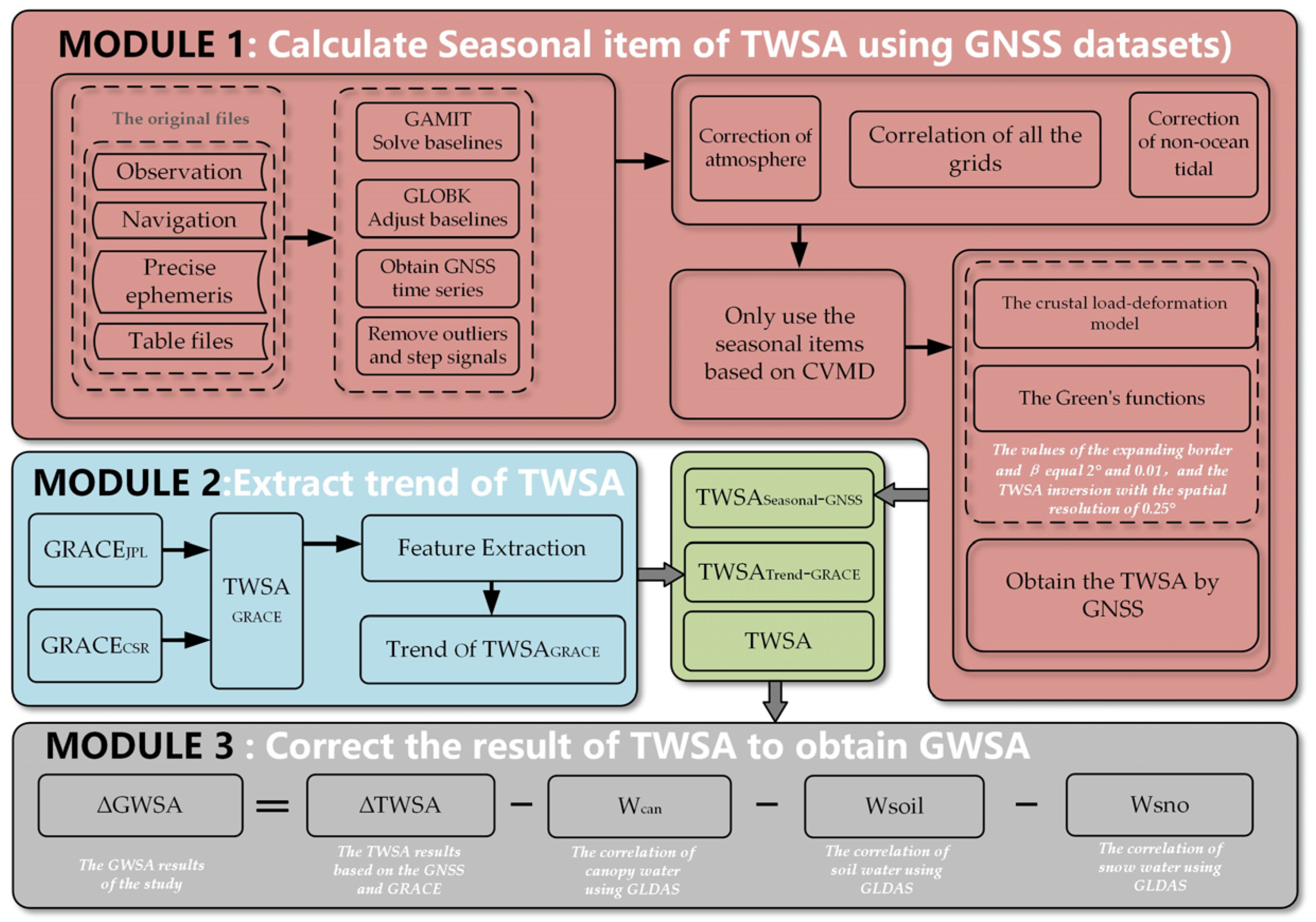
To take full advantage of the high spatiotemporal resolutions provided by GNSS data, as well as the ability of GRACE to accurately monitor ground water dynamics, the seasonal terms of TWSA in the NCP region were derived by using the GNSS vertical series, and the trend term of TWSA was determined by using GRACE mascon data. The GWSA was then calculated by subtracting values for canopy water, soil water, and snow water.

(2)

This study inverted the TWSA based on the 26 GNSS vertical sequences provided by CMONOC over NCP. The TWSA results shows that the TWSA amplitude is higher than that of 2011~2014, which is consistent with the timing of South–North Water Transfer Project. Meanwhile, the maximum annual amplitude of the TWSA result is 170 mm, which is higher than that of the maximum semiannual amplitude of TWSA. The results of TWSA sequences are the basis of the inversion for GWSA.

(3)

To verify the reliability of the inverted method by combining the GNSS, GRACE/GRACE-FO, and GLDAS, the experimental results were compared with the GWSA variables in the GLDAS datasets. The comparison results show that the amplitude peaks are located in the Beijing and Tianjin regions, and the spatial features of the trend terms show that the high anomalies are located in the north and south of the NCP, and the low anomalies are found in the middle of the NCP. The PCC, RMSE, and NSE values are 0.67, 4.01 cm, and 0.61, respectively, while the superimposed power spectra showed that the two sequences are consistent at low and medium frequencies. Therefore, the inversion methodology proposed in this study is a reliable way of determining regional GWSA.

(4)

Using the GWSA inversion results obtained in this study, we analyzed the groundwater drought and the impact of the South–North Water Transfer Project on groundwater storage in the NCP from 2011 to 2021. The most obvious groundwater drought year in the NCP was 2019, with a DSI value of −0.12, which was close to moderate drought conditions. Moreover, the DSI value reached −0.81 in 2017, which was indicative of mild drought conditions. The South–North Water Transfer Project officially opened for water transmission at the end of 2014, and the annual GWSA amplitude increased significantly compared with that before the opening of the South–North Water Transfer Project. This suggests that the demand for land water from industry and agriculture increased after the transfer. Additionally, there is a significant amplitude increase in the Tianjin and Hebei regions between 2015 and 2020, indicating that the demand for groundwater in this region is higher than in other regions. In conclusion, the South–North Water Transfer Project does have an impact on groundwater storage in Hebei Province.

References

1. Feng, W.; Zhong, M.; Lemoine, J.M.; Biancale, R.; Hsu, H.T.; Xia, J. Evaluation of groundwater depletion in north China using the gravity recovery and climate experiment (GRACE) data and ground-based measurements. Water Resour. Res. 2013, 49, 2110–2118. [Google Scholar] [CrossRef]
2. Zhong, Y.; Zhong, M.; Feng, W.; Zhang, Z.; Shen, Y.; Wu, D. Groundwater Depletion in the West Liaohe River Basin, China and Its Implications Revealed by GRACE and In Situ Measurements. Remote Sens. 2018, 10, 493. [Google Scholar] [CrossRef] [Green Version]
3. Yin, W.; Hu, L.; Zhang, M.; Wang, J.; Han, S. Statistical downscaling of GRACE-derived groundwater storage using ET data in the north China plain. J. Geophys. Res. Atmos. 2018, 123, 5973–5987. [Google Scholar] [CrossRef]
4. Davis, J.L.; Tamisiea, M.E.; Elosegui, P.; Mitrovica, J.X.; Hill, E.M. A statistical filtering approach for Gravity Recovery and Climate Experiment (GRACE) gravity data. J. Geophys. Res.-Solid Earth 2008, 113, 1–14. [Google Scholar] [CrossRef] [Green Version]
5. Pang, Y.; Zhang, H.; Cheng, H.; Shi, Y. Changes of crustal stress induces by groundwater over-puming in North China Plain. Chin. J. Geophy. 2016, 59, 1394–1402. [Google Scholar]
6. Long, D.; Shen, Y.; Sun, A.; Hong, Y.; Longuevergne, L.; Yang, Y.; Li, B.; Chen, L. Drought and flood monitoring for a large karst plateau in southwest China using extended GRACE data. Remote Sens. Environ. 2014, 155, 145–160. [Google Scholar] [CrossRef]
7. Scanlon, B.R.; Zhang, Z.; Save, H.; Wiese, D.N.; Landerer, F.W.; Long, D.; Longuevergne, L.; Chen, J. Global evaluation of new GRACE mascon products for hydrologic applications. Water Resour. Res. 2016, 52, 9412–9429. [Google Scholar] [CrossRef] [Green Version]
8. Li, W.; Wang, W.; Zhang, C.; Wen, H.; Zhong, Y.; Zhu, Y.; Li, Z. Bridging terrestrial water storage anomaly during GRACE/GRACE-FO gap using SSA method: A case study in China. Sensors 2019, 19, 4144. [Google Scholar] [CrossRef] [Green Version]
9. Zheng, W.; Hsu, H.; Zhong, M.; Yun, M. Requirements analysis for future satellite gravity mission improved-GRACE. Surv. Geophys. 2015, 36, 87–109. [Google Scholar] [CrossRef]
10. Zheng, W.; Lu, X.; Hsu, H.; Shao, C.; Luo, J.; Wang, N. Simulation of the Earth’s gravitational field recovery from GRACE using the energy balance approach. Prog. Nat. Sci. 2005, 15, 596–601. [Google Scholar]
11. Tangdamrongsub, N.; Ditmar, P.G.; Steele-Dunne, S.C.; Gunter, B.C.; Sutanudjaja, E.H. Assessing total water storage and identifying flood events over Tonlé Sap basin in Cambodia using GRACE and MODIS satellite observations combined with hydrological models. Remote Sens. Environ. 2016, 181, 162–173. [Google Scholar] [CrossRef] [Green Version]
12. Tan, W.J.; Dong, D.A.; Chen, J.P.; Wu, B. Analysis of systematic differences from GPS-measured and GRACE-modeled deformation in Central Valley, California. Adv. Space Res. 2016, 57, 19–29. [Google Scholar] [CrossRef]
13. Liu, Z.; Liu, P.W.; Massoud, E.; Farr, T.G.; Lundgren, P.; Famiglietti, J.S. Monitoring groundwater change in California’s central valley using Sentinel-1 and GRACE observations. Geosciences 2019, 9, 436. [Google Scholar] [CrossRef] [Green Version]
14. Yin, W.; Hu, L.; Jiao, J.J. Evaluation of groundwater storage variations in northern China using GRACE data. Geofluids 2017, 2017, 8254824. [Google Scholar] [CrossRef] [Green Version]
15. Zhao, Q.; Zhang, B.; Yao, Y.B.; Wu, W.W.; Meng, G.J.; Chen, Q. Geodetic and hydrological measurements reveal the recent acceleration of groundwater depletion in north China plain. J. Hydrol. 2019, 575, 1065–1072. [Google Scholar] [CrossRef]
16. Li, W.Q.; Wang, W.; Zhang, C.Y.; Yang, Q.; Feng, W.; Liu, Y. Monitoring groundwater storage variations in the Guanzhong area using GRACE satellite gravity data. Chin. J. Geophys. 2018, 61, 67–75. [Google Scholar]
17. Nie, N.; Zhang, W.; Zhang, Z.; Guo, H.; Ishwaran, N. Reconstructed terrestrial water storage change (ΔTWS) from 1948 to 2012 over the Amazon basin with the latest GRACE and GLDAS products. Water Resour. Manag. 2016, 30, 279–294. [Google Scholar] [CrossRef]
18. Cui, L.L.; Song, Z.; Luo, Z.C.; Zhong, B.; Wang, X.L.; Zou, Z.B. Comparison of terrestrial water storage changes derived from GRACE/GRACE-FO and Swarm: A case study in the Amazon river basin. Water 2020, 12, 3128. [Google Scholar] [CrossRef]
19. Flechtner, F.; Neumayer, K.H.; Dahle, C.; Dobslaw, H.; Fagiolini, E.; Raimondo, J.C.; Guntner, A. What Can be Expected from the GRACE-FO Laser Ranging Interferometer for Earth Science Applications? Surv. Geophys. 2016, 37, 453–470. [Google Scholar] [CrossRef] [Green Version]
20. Zhong, Y.; Zhong, M.; Mao, Y.; Ji, B. Evaluation of Evapotranspiration for Exorheic Catchments of China during the GRACE Era: From a Water Balance Perspective. Remote Sens. 2020, 12, 1–23. [Google Scholar] [CrossRef] [Green Version]
21. Landerer, F.W.; Swenson, S.C. Accuracy of scaled GRACE terrestrial water storage estimates. Water Resour. Res. 2012, 48, W04531. [Google Scholar] [CrossRef]
22. Fu, Y.N.; Freymueller, J.T.; Jensen, T. Seasonal hydrological loading in southern Alaska observed by GPS and GRACE. Geophys. Res. Lett. 2012, 39, 1–5. [Google Scholar] [CrossRef] [Green Version]
23. Shen, Y.; Zheng, W.; Yin, W.; Xu, A.; Zhu, H.; Yang, S.; Su, K. Inverted algorithm of terrestrial water-storage anomalies based on machine learning combined with load model and its application in southwest China. Remote Sens. 2021, 13, 3358. [Google Scholar] [CrossRef]
24. Adusumilli, S.; Borsa, A.A.; Fish, M.A.; McMillan, H.K.; Silverii, F. A decade of water storage changes across the contiguous united states from GPS and satellite gravity. Geophys. Res. Lett. 2019, 46, 13006–13015. [Google Scholar] [CrossRef]
25. Carlson, G.; Werth, S.; Shirzaei, M. Joint Inversion of GNSS and GRACE for Terrestrial Water Storage Change in California. J. Geophys. Res. Solid Earth 2022, 127, 1–24. [Google Scholar] [CrossRef] [PubMed]
26. Godah, W. Comparison of vertical deformation of the Earth_s surface obtained using GRACE_based GGMS and GNNS data _ a case study of South_Eastern Poland. Acta Geodyn. Geomater. 2020, 2, 169–176. [Google Scholar] [CrossRef]
27. Shen, Y.; Zheng, W.; Yin, W.; Xu, A.; Zhu, H. Feature extraction algorithm using a correlation coefficient combined with the VMD and its application to the GPS and GRACE. IEEE Access 2021, 9, 17507–17519. [Google Scholar] [CrossRef]
28. Shen, Y.; Zheng, W.; Yin, W.; Xu, A.; Zhu, H.; Wang, Q.; Chen, Z. Improving the inversion accuracy of terrestrial water storage anomaly by combining GNSS and LSTM algorithm and its application in mainland China. Remote Sens. 2022, 14, 535. [Google Scholar] [CrossRef]
29. Wang, H.; Xiang, L.; Jia, L.; Jiang, L.; Wang, Z.; Bo, H.; Peng, G. Load love numbers and Green’s functions for elastic earth models PREM, iasp91, ak135, and modified models with refined crustal structure from Crust 2.0. Comput. Geosci. 2012, 49, 190–199. [Google Scholar] [CrossRef]
30. Martens, H.R.; Rivera, L.; Simons, M. LoadDef: A python-based toolkit to model elastic deformation caused by surface mass loading on spherically symmetric bodies. Earth Space Sci. 2019, 6, 311–323. [Google Scholar] [CrossRef] [Green Version]
31. Dill, R.; Klemann, V.; Martinec, Z.; Tesauro, M. Applying local Green’s functions to study the influence of the crustal structure on hydrological loading displacements. J. Geodyn. 2015, 88, 14–22. [Google Scholar] [CrossRef] [Green Version]
32. Dach, R.; Böhm, J.; Lutz, S.; Steigenberger, P.; Beutler, G. Evaluation of the impact of atmospheric pressure loading modeling on GNSS data analysis. J. Geod. 2011, 85, 75–91. [Google Scholar] [CrossRef] [Green Version]
33. Sheng, C.Z.; Gan, W.J.; Liang, S.M.; Chen, W.T.; Xiao, G.R. Identification and elimination of non-tectonic crustal deformation caused by land water from GPS time series in the western Yunnan province based on GRACE observations. Chin. J. Geophys. 2014, 57, 42–52. [Google Scholar] [CrossRef]
34. Zhang, B.; Yao, Y.B.; Fok, H.S.; Hu, Y.F.; Chen, Q. Potential Seasonal Terrestrial Water Storage Monitoring from GPS Vertical Displacements: A Case Study in the Lower Three-Rivers Headwater Region, China. Sensors 2016, 16, 1526. [Google Scholar] [CrossRef]
35. Xu, H.; Lu, T.; Montillet, J.P.; He, X. An improved adaptive IVMD-WPT-Based noise reduction algorithm on GPS height time series. Sensors 2021, 21, 8295. [Google Scholar] [CrossRef]
36. Wu, S.G.; Li, Z.; Li, H.P.; Nie, G.G.; Liu, J.N.; He, Y.F. Application of an improved clustering approach on GPS height time series at CMONOC stations in southwestern China. Earth Planets Space 2021, 73, 233. [Google Scholar] [CrossRef]
37. Jiang, Z.; Hsu, Y.-J.; Yuan, L.; Huang, D. Monitoring time-varying terrestrial water storage changes using daily GNSS measurements in Yunnan, southwest China. Remote Sens. Environ. 2021, 254, 112249–112266. [Google Scholar] [CrossRef]
38. Ding, Y.H.; Huang, D.f.; Shi, Y.L.; Jiang, Z.S.; Chen, T. Determination of vertical surface displacements in Sichuan using GPS and GRACE measurements. Chin. J. Geophys. 2018, 61, 4777–4788. [Google Scholar]
39. Liu, R.; Zou, R.; Li, J.; Zhang, C.; Zhao, B.; Zhang, Y. Vertical displacements driven by groundwater storage changes in the north China plain detected by GPS observations. Remote Sens. 2018, 10, 259. [Google Scholar] [CrossRef] [Green Version]
40. Abdrakhmatov, K.Y.; Aldazhanov, S.A.; Hager, B.H.; Hamburger, M.W.; Herring, T.A.; Kalabaev, K.B.; Makarov, V.I.; Molnar, P.; Panasyuk, S.V.; Prilepin, M.T.; et al. Relatively recent construction of the Tien Shan inferred from GPS measurements of present-day crustal deformation rates. Nature 1996, 384, 450–453. [Google Scholar] [CrossRef]
41. Sun, W.K.; Wang, Q.; Li, H.; Wang, Y.; Okubo, S. A reinvestigation of crustal thickness in the Tibetan Plateau using absolute gravity, GPS and GRACE data. Terr. Atmos. Ocean. Sci. 2011, 22, 109–119. [Google Scholar] [CrossRef] [Green Version]
42. Sun, W.K.; Zhou, X. Advances, problems and prospects of modern geodesy applied in Tibetan geodynamic changes. Acta Geol. Sin. 2013, 87, 318–332. [Google Scholar] [CrossRef]
43. Chen, C.; Wang, T.; Linsong, D.; Jin, S. Detecting seasonal and long-term vertical displacement in the north China plain using GRACE and GPS. Hydrol. Earth Syst. Sci. 2017, 21, 2905–2922. [Google Scholar]
44. Long, D.; Yang, W.; Scanlon, B.R.; Zhao, J.; Liu, D.; Burek, P.; Pan, Y.; You, L.; Wada, Y. South-to-North water diversion stabilizing Beijing’s groundwater levels. Nat. Commun. 2020, 11, 3665–3675. [Google Scholar] [CrossRef] [PubMed]
45. Liu, C.; Zheng, H. South-to-north Water Transfer Schemes for China. Int. J. Water Resour. Dev. 2002, 18, 453–471. [Google Scholar] [CrossRef]
46. Wang, W.; Zhao, B.; Wang, Q.; Yang, S. Noise analysis of continuous GPS coordinate time series for CMONOC. Adv. Space Res. 2012, 49, 943–956. [Google Scholar] [CrossRef]
47. Herring, T.A.; King, R.W.; Mcclusky, S.C. GAMIT Reference Manual; Massachussetts Institute Technology: Cambridge, UK, 2010. [Google Scholar]
48. Xiang, Y.F.; Yue, J.P.; Li, Z. Joint analysis of seasonal oscillations derived from GPS observations and hydrological loading for mainland China. Adv. Space Res. 2018, 62, 3148–3161. [Google Scholar] [CrossRef]
49. Han, S.-C.; Shum, C.K.; Jekeli, C.; Kuo, C.-Y.; Wilson, C.; Seo, K.-W. Non-isotropic filtering of GRACE temporal gravity for geophysical signal enhancement. Geophys. J. Int. 2005, 163, 18–25. [Google Scholar] [CrossRef] [Green Version]
50. Long, D.; Longuevergne, L.; Scanlon, B.R. Uncertainty in evapotranspiration from land surface modeling, remote sensing, and GRACE satellites. Water Resour. Res. 2014, 50, 1131–1151. [Google Scholar] [CrossRef] [Green Version]
51. Saito, M. Relationship Between Tidal and Load Love Numbers. J. Phys. Earth 1978, 26, 13–16. [Google Scholar] [CrossRef]
52. Cheng, M.; Ries, J.C.; Tapley, B.D. Variations of the Earth’s figure axis from satellite laser ranging and GRACE. J. Geophys. Res. 2011, 116, 1–14. [Google Scholar] [CrossRef] [Green Version]
53. Li, J.; Chen, J.; Li, Z.; Wang, S.-Y.; Hu, X. Ellipsoidal Correction in GRACE Surface Mass Change Estimation. J. Geophys. Res. Solid Earth 2017, 122, 9437–9460. [Google Scholar] [CrossRef]
54. Rodell, M.; Houser, P.R.; Jambor, U.; Gottschalck, J.; Mitchell, K.; Meng, C.J.; Arsenault, K.; Cosgrove, B.; Radakovich, J.; Bosilovich, M.; et al. The Global Land Data Assimilation System. Bull. Am. Meteorol. Soc. 2004, 85, 381–394. [Google Scholar] [CrossRef] [Green Version]
55. Li, B.; Rodell, M.; Kumar, S.; Beaudoing, H.K.; Getirana, A.; Zaitchik, B.F.; Goncalves, L.G.; Cossetin, C.; Bhanja, S.; Mukherjee, A.; et al. Global GRACE Data Assimilation for Groundwater and Drought Monitoring: Advances and Challenges. Water Resour. Res. 2019, 55, 7564–7586. [Google Scholar] [CrossRef] [Green Version]
56. Tesmer, V.; Steigenberger, P.; Dam, T.V.; Mayer-Guerr, T. Vertical deformations from homogeneously processed GRACE and global GPS long-term series. J. Geod. 2011, 85, 291–310. [Google Scholar] [CrossRef]
57. Farrell, W.E. Deformation of the earth by surface loads. Rev. Geophys. 1972, 10, 761–797. [Google Scholar] [CrossRef]
58. Wang, X.; Chen, L.; Ai, Y.; Xu, T.; Jiang, M.; Yuan, L.; Gao, Y. Crustal structure and deformation beneath eastern and northeastern Tibet revealed by P-wave receiver functions. Earth Planet. Sci. Lett. 2018, 497, 69–79. [Google Scholar] [CrossRef]
59. Wahr, J.; Khan, S.A.; Dam, T.V.; Liu, L.; Angelen, J.V.; Van, D.; Meertens, C.M. The use of GPS horizontals for loading studies, with applications to northern California and southeast Greenland. J. Geophys. Res. Solid Earth 2013, 118, 1795–1806. [Google Scholar] [CrossRef] [Green Version]
60. Springer, A.; Karegar, M.A.; Kusche, J.; Kurtz, W.; Kollet, S. Evidence of daily hydrological loading in GPS time series over Europe. J. Geod. 2019, 93, 2145–2153. [Google Scholar] [CrossRef]
61. Wang, Z.; Ou, J. Determining the ridge parameter in a ridge estimation using L-curve method. Editor. Board Geomat. Inf. Sci. Wuhan Univ. 2004, 29, 235–238. [Google Scholar]
62. Liesch, T.; Ohmer, M. Comparison of GRACE data and groundwater levels for the assessment of groundwater depletion in Jordan. Hydrogeol. J. 2016, 24, 1547–1563. [Google Scholar] [CrossRef]
63. Han, Z.; Huang, S.; Huang, Q.; Leng, G.; Wang, H.; Bai, Q.; Zhao, J.; Ma, L.; Wang, L.; Du, M. Propagation dynamics from meteorological to groundwater drought and their possible influence factors. J. Hydrol. 2019, 578, 124102. [Google Scholar] [CrossRef]
64. Chai, T.; Draxler, R.R. Root mean square error (RMSE) or mean absolute error (MAE) aguments against avoiding RMSE in the literature. Geosci. Model Dev. 2014, 7, 1247–1250. [Google Scholar] [CrossRef] [Green Version]
65. Gupta, H.V.; Kling, H.; Yilmaz, K.K.; Martinez, G.F. Decomposition of the mean squared error and NSE performance criteria: Implications for improving hydrological modelling. J. Hydrol. 2009, 377, 80–91. [Google Scholar] [CrossRef] [Green Version]
66. Yu, J.; Tan, K.; Zhang, C.; Zhao, B.; Wang, D.; Li, Q. Present-day crustal movement of the Chinese mainland based on Global Navigation Satellite System data from 1998 to 2018. Adv. Space Res. 2019, 63, 840–856. [Google Scholar] [CrossRef]
67. Gong, H.; Pan, Y.; Zheng, L.; Li, X.; Zhu, L.; Zhang, C.; Huang, Z.; Li, Z.; Wang, H.; Zhou, C. Long-term groundwater storage changes and land subsidence development in the North China Plain (1971–2015). Hydrogeol. J. 2018, 26, 1417–1427. [Google Scholar] [CrossRef]
68. Moiwo, J.P.; Tao, F.; Lu, W. Analysis of satellite-based and in situ hydro-climatic data depicts water storage depletion in North China Region. Hydrol. Process. 2013, 27, 1011–1020. [Google Scholar] [CrossRef]
69. Huang, Z.; Pan, Y.; Gong, H.; Yeh, P.J.F.; Li, X.; Zhou, D.; Zhao, W. Subregional-scale groundwater depletion detected by GRACE for both shallow and deep aquifers in North China Plain. Geophys. Res. Lett. 2015, 42, 1791–1799. [Google Scholar] [CrossRef]
70. Li, P.; Zha, Y.; Shi, L.; Zhong, H. Identification of the terrestrial water storage change features in the North China Plain via independent component analysis. J. Hydrol. Reg. Stud. 2021, 38, 100955. [Google Scholar] [CrossRef]
71. Zhang, C.; Duan, Q.; Yeh, P.J.-F.; Pan, Y.; Gong, H.; Moradkhani, H.; Gong, W.; Lei, X.; Liao, W.; Xu, L.; et al. Sub-regional groundwater storage recovery in North China Plain after the South-to-North water diversion project. J. Hydrol. 2021, 597, 126156. [Google Scholar] [CrossRef]
Figure 1. Map of GNSS station locations in the NCP: (a) depicts the specific location of the North China Plain; (b) shows the distribution of GNSS stations, the digital elevation model (DEM) information, and the rivers over NCP.
Remotesensing 14 05683 g001
Figure 2. Flow chart showing the processes and operations in this study.
Remotesensing 14 05683 g002
Figure 3. TWSA spatiotemporal distribution derived by GNSS inversion: (a) TWSA time series of the North China Plain, (b) TWSA annual amplitude spatial and temporal distribution, (c) TWSA semiannual amplitude spatiotemporal distribution.
Remotesensing 14 05683 g003
Figure 4. TWSA plots from the fused GNSS and GRACE/GRACE-FO data: (a) TWSA time series, (b) indicates the annual TWSA term in GLDAS dataset, (c) indicates the trend term of TWSA in GLDAS dataset, (d) indicates the trend term of the TWSA results from the fused GNSS and GRACE data, (e) indicates the scatter plot of experimental results and GLDAS in this study.
Remotesensing 14 05683 g004
Figure 5. The GWSA inversion results: (a) GWSA daily slice plot, (b) GWSA annual amplitude plot, (c) time series of GWSA average sequence.
Remotesensing 14 05683 g005
Figure 6. Comparison plots of GWSA inversion results: (a) GLDAS annual amplitude, (b) GLDAS trend plot, (c) trend plot of inversion results using the method presented in this study, (d) sequence comparison effect plot, (e) superimposed power spectrum.
Remotesensing 14 05683 g006
Figure 7. Drought severity index map of groundwater storage: (ak) spatial distribution of DSI in the NCP between 2011 and 2021, (l) DSI sequence change map.
Remotesensing 14 05683 g007
Figure 8. Spatial distribution and time series of GWSA in the NCP between 2011 and 2021 (ak).
Remotesensing 14 05683 g008