Monitoring Ecological Changes on a Rapidly Urbanizing Island Using a Remote Sensing-Based Ecological Index Produced Time Series

Abstract

Island ecosystems are susceptible to the considerable impacts of increasing human activities, landscape reconstruction, and urban expansion, resulting in changes in the ecological environment and urban ecological security issues. Remote sensing techniques can achieve the near-real-time ecological environment monitoring of these rapidly changing areas. The remote sensing-based ecological index (RSEI), as a comprehensive remote sensing ecological environment index, was adopted to dynamically monitor urban ecological quality (EQ) over time in this study, combined with the Landsat-based detection of trends in disturbance and recovery (LandTrendr) algorithm. Annual composite images were generated using Landsat 5, Landsat 7, and Landsat 8 imagery to extract four metrics (Greenness, Moisture, Heat, and Dryness) to calculate RSEI from 1991 to 2021. The ecological quality in the study area was evaluated using a five-level classification (poor, inferior, medium, good, and excellent), and the changes in EQ on a pixel basis were identified by the LandTrendr algorithm. The results showed that (1) the average value of the RSEI ranged from 0.47 to 0.57 over 31 years, indicating that EQ was maintained at the medium level; (2) the distribution of different EQ levels had visible patterns, and an area of 47.87 km² was affected by a poor EQ at least once in 31 years; (3) 38.22 km² of this area experienced EQ poor disturbance once, and 3.05 km² of the area had poor disturbance twice. Urban expansion, forest degradation, and policy are the main factors causing the reduction of the RSEI. The results demonstrate that combining time series of RSEI and LandTrendr can effectively monitor the changes of EQ, which is helpful to identify the spatial–temporal variation patterns of EQ and provide valuable information for policymakers and protection.

1. Introduction

Islands have a sensitive ecosystem due to their particular geographical location and unique resources [1,2]. Currently, island ecosystems are confronted with increasing human activities, such as overpopulation, land use change, and tourism activities. Those activities can trigger irreversible damage to the ecological environment [3]. In order to effectively assess the quality of the ecological environment for humankind and maintain the sustainable development of islands, it is necessary to detect ecological quality (EQ), particularly the long-term dynamics of the ecological environment.

There are many methods to detect EQ. For example, the ecological environment for all the provinces and three economic regions in China was assessed by Sun et al. using an Analytic Hierarchy Process [4]. Wu et al. used a fuzzy integrated assessment method to evaluate the EQ of three semi-enclosed coastal areas [5]. However, the evaluation of the ecological environment based on traditional semi-quantitative methods was limited because it did not detect the EQ rapidly and in near real-time. Remote sensing-based data and technologies have been proven as an effective, rapid, and near-real-time method, which has been widely applied for ecological environment monitoring at different scales [6]. Mainly, remote sensing technology provides multiple tools and algorithms to support ecological detection [7,8]. Xiong et al. assessed the spatial–temporal changes of EQ in the Erhai lake basin based on Landsat imagery [9]. Coupled with several indices, the ecological environment in the Heihe river basin was evaluated by Wang et al. [10]. In addition, remote sensing techniques can be applied for long-term series ecological environment monitoring with the advantage of spatial and temporal consistency.

For the remote sensing evaluation of the ecological environment, a number of remote sensing-based indices have been used in previous studies. For example, the Normalized Difference Vegetation Index (NDVI) was often used to detect vegetation change and reflect environmental changes [11,12]. Similarly, the Leaf Area Index (LAI) [13,14], and the Enhanced Vegetation Index (EVI) [15], which are also vegetation indices, were used to assess the vegetation changes of the ecological environment. Other single indices, such as the Permanent Vegetation Fraction (PVF) [16], the Ratio Drought Index (RDI) [17], and the Standardized Precipitation Index (SPI) [18], were developed to characterize related aspects of the ecological environment. However, single indices have limitations for evaluating the EQ due to the diversity and complexity of the ecological environment. Therefore, several aggregated ecological indices have also been created and utilized to explore ecological environment changes, which can identify and reflect more features related to EQ (e.g., the scaled drought condition index (SDCI) [19], the frequently used forest disturbance index (DI), the MODIS global disturbance index (MGDI) [20], the ecological index (EI) [7], and the remote sensing-based ecological index (RSEI) [21,22]). Particularly, RSEI is a newly developed aggregated index that has been used to detect EQ solely based on remote sensing imagery [8,23]. The RSEI encompasses four metrics (Greenness, Moisture, Heat, and Dryness), which are closely related to the ecological environment caused by human activities and can be perceived by humans. Moreover, the weight of each metric can be determined by principal component analysis (PCA) without human subjective analysis. The credibility and reliability of RSEI were verified in previous studies [24] and it has been widely used in the evaluation of islands [25], basins [9,21], cities [26], and watershed areas [27,28]. Xu et al. used RSEI to predict the ecological effects caused by potential population and impervious surface increases, which yielded an average RSEI of 0.645 for the whole area and an average RSEI of 0.402 for the impervious built area in the Xiong’an New Area [29]. Shan et al. assessed EQ using RSEI, and provided a contrastive analysis between RSEI (65.200, 57.200, 60.500) and EI (65.775, 62.113, 62.113) at the centesimal system before, during, and after land consolidation [7].

However, the application of RSEI for EQ assessment has relied on multiple remote sensing images in two or more different time periods in previous studies [7,9,26]. For instance, Geng at el. assessed the EQ of Fuzhou City from 2000 to 2020 for five periods (2000, 2005, 2010, 2015, and 2020), but it was insufficient to reflect the continuous long-term series of ecological changes. The time series trajectory analysis method can better capture the detailed changes in EQ [30]. Particularly, the Landsat archive is suitable for long-term assessment because it holds nearly 50 years of continuous data with a 16-day revisit cycle and multispectral high-resolution images (30 m) [6]. As a free and cloud-computing platform, the Google Earth Engine (GEE) (https://earthengine.google.com/, accessed on 8 October 2020) provides various remote sensing image archives and can assist with long-time EQ detection [6,31,32,33]. The GEE platform can handle the dense Landsat data computations and provides multiple algorithms to support image processing, including filter image collection, cloud masking, and image composite functions. In addition, corresponding time series data analysis methods have been developed, such as Change Vector Analysis (CVA) [34,35,36], Continuous Change Detection and Classification (CCDC) [37], and other algorithms [30,38,39]. The LandTrendr algorithm was proposed by Kennedy et al. for monitoring forest disturbance [40]. Later, this algorithm was developed and applied for detecting other aspects of annual changes, such as mangrove dynamics [41], permafrost thaw [6], marsh vegetation, and hydrology change [42]. LandTrendr is one of the optimal algorithms to detect long-term series dynamic change on a pixel basis [40]. It is able to detect drastic short-term changes of the target object within the image, and can also distinguish long-term ecological recovery [40]. However, there are few studies that have used LandTrender to analyze the changes of EQ in a continuous time series.

In this study, the main objectives are to quantify the spatio–temporal variation patterns of EQ, and explore the changes of EQ over the past 31 years (1991–2021) using the annual time series trajectory method for Haitan Island. As the fifth-largest island in China, Haitan Island has experienced unprecedented changes over the past 30 years [3]. Haitan Island’s originally fragile ecosystem has attracted increasing attention due to its strategic position on southeast trade routes. On Haitan Island, a coastal shelter forest was planted by the government between 1988 and 2005 to protect the ecological environment. Subsequently, a ‘Comprehensive Pilot Zone’ program was proposed in 2009, a free trade zone was set up in 2014, and the ‘Pingtan National Tourism Island Construction Plan’ was launched in 2016 to boost the economy and social development. As a result, urbanization, tourism, and commercialization were subsequently accelerated [3]. In this context, anthropogenic activities continuously impact the ecological system of Haitan Island. Therefore, it is necessary to understand the changes in ecological environment fully. The main scientific questions are as follows:

(1)

How can the RSEI data be determined from the annual Landsat time series images of Haitan Island (1991–2021)?

(2)

How can the changes in the spatial patterns of EQ be quantified over time?

2. Materials and Methods

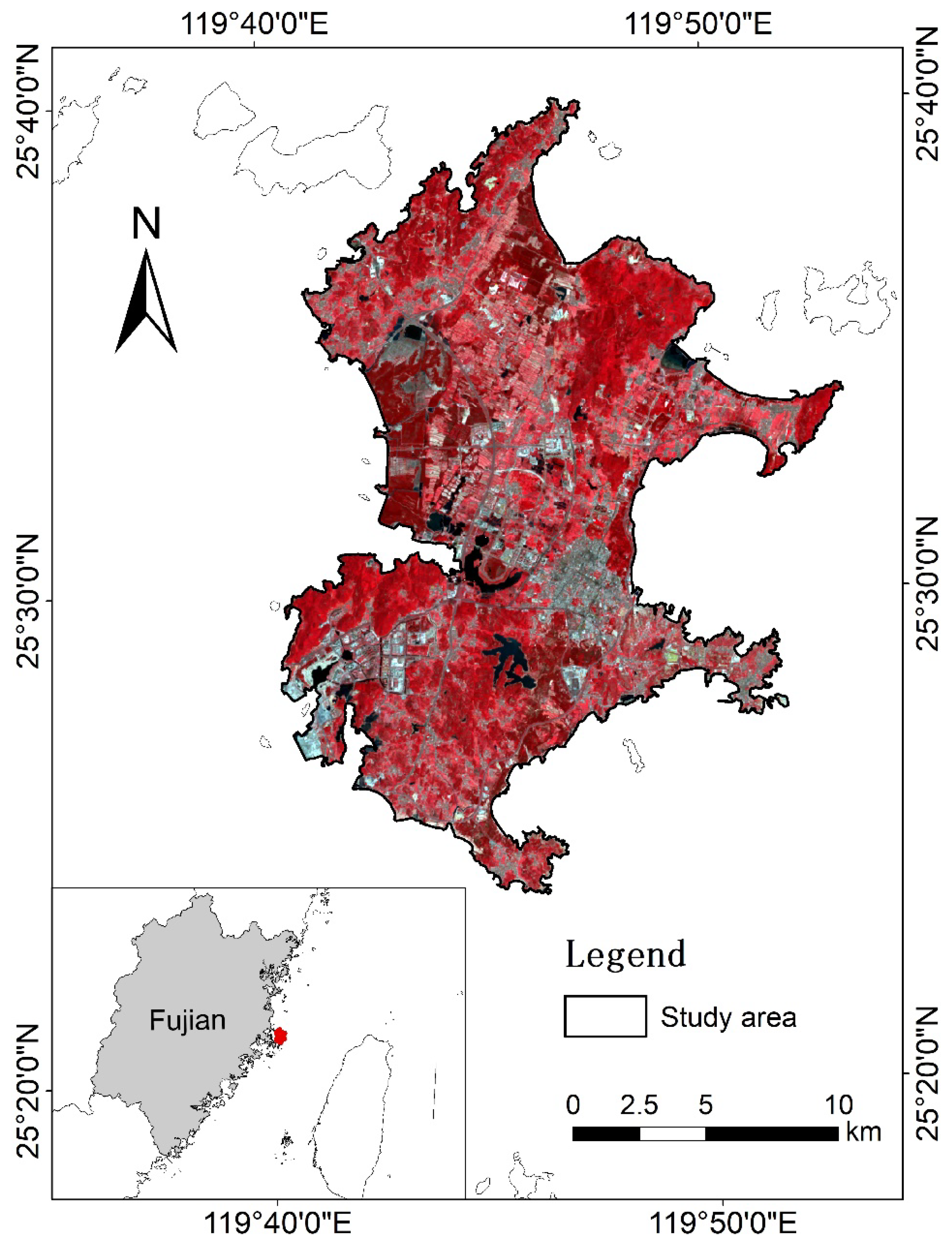
2.1. Study Site

Haitan Island is located in the Pingtan Comprehensive Pilot Zone, Fujian, China (coordinates: 25°15′N–25°45′N, 119°32′E–120°10′E) (Figure 1). It covers about 267 km² of land area, with a permanent population of 385,981 in 2020. Haitan Island is divided into seven towns and four villages. Marine accumulation plains characterize the Haitan Island terrain. The north and south of the island are mostly mountainous and hilly, and the middle area is a plain. Junshan mountain (434.40 m) has the highest elevation on the island. The average annual temperature is 19.8 °C, with around 33–37 °C in the hottest month (between July and August). The average annual precipitation is 1000–1200 mm. The island faces heavy rainstorms and wind erosion due to its location, and is prone to severe soil loss.

2.2. Data Sources and Pre-Processing

Landsat has the longest continuous multi-spectral image archive, which is well suited for long-term ecological observation. In this study, Landsat 5, Landsat 7, and Landsat 8 imagery Surface Reflectance Tier 1 from 1991 to 2021, provided by the U.S. Geological Survey Center in the GEE platform, were obtained, which included three scene centers (path/row: 118/42, 118/43, 119/42). The visible, near-infrared, mid-infrared, and thermal infrared bands from Landsat 5, Landsat 7, and Landsat 8 were used in this study (bands 1–7 for Landsat 5, Landsat 7 and bands 2–7, 10 for Landsat 8) [43]. In all, 1286 Landsat 5 scenes from 1991 to 2011, 30 Landsat 7 scenes from 2012, and 453 Landsat 8 scenes from 2013 to 2021 were collected (Figure 2). Moreover, the spatial resolution of all images was resampled to 30 m due to the thermal infrared band having a lower resolution.

Figure 1. Location of Haitan, Fujian, China and its composite Landsat image (2021).

Figure 1. Location of Haitan, Fujian, China and its composite Landsat image (2021).

Image preprocessing, including image time screening, cloud and cloud shadow removal, multi-dimensional median (medoid) technique, and time series interpolation, was applied to produce the cloud-free, high quality, and representative annual mosaic images for Haitan Island.

First, to improve the quality and comparability of the remote sensing data, the images from May to October were selected because the differences in solar angles and vegetation phenology can be minimized for images obtained during the vegetation growing season. Second, the cloud and cloud shadow pixels were masked based on Landsat band: BQA (CFMASK), and images with cloud coverage of less than 30% were initially filtered [44,45].

The medoid mosaicking function was applied to produce the combined annual mosaiced image [46,47]. The medoid technique chooses the pixel value with a minimum sum of squared differences between observations and the median values across bands. This method ensures robustness and preserves the relationships between bands due to the selected pixel values being one of that pixel’s observations [47].

Additionally, if the cloud and cloud shadows still exist in a location among all images for a year, there are no suitable images available for this location. This could result in missing data in the annual mosaic image. To ensure the continuity in time series image collections from 1991 to 2021, missing data were filled with the mean value of the band in adjacent years based on the method of Robinson et al. [48]. All processing was completed on the GEE platform.

2.3. Methods

2.3.1. Calculation of Remote Sensing-Based Ecological Index (RSEI)

In this study, RSEI was applied to detect the EQ [24] of Haitan Island from 1991 to 2021. Initially, to avoid the influence of water area on the RSEI, Modified Normalized Difference Water Index (MNDWI) [49] was used to remove the water area from the Landsat imagery (Equation (1)).

$$MNDWI=\left(Green-SWIR1\right)/\left(Green+SWIR1\right)$$

(1)

where Green and SWIR1 are the values of green and short-wavelength infrared 1 band in the Landsat image, respectively.

Four metrics, including Greenness, Moisture, Heat, and Dryness, involved in RSEI (Equation (2)), were calculated. The Greenness index represents vegetation, which can be calculated using the Normalized Difference Vegetation Index (NDVI). The Moisture index represents soil moisture, which can be calculated by the wet component using a Tasseled Cap Transformation. The Heat index represents temperature, which can be shown by land surface temperature (LST). The Dryness index mainly refers to bare soil and built area, which can be shown by Normalized Difference Impervious Surface Index (NDISI). NDVI, Wet, LST, and NDBI were calculated as follows (

Table 1. The formulae and explanations of four metrics in RSEI.

Indicator	Calculation Method	Explanation
NDVI	$NDVI=\left(NIR-Red\right)/\left(NIR+Red\right)$	NIR and Red are the values of near-infrared and red band in the Landsat image, respectively.
WET	$We{t}_{TM}=0.0315\times Blue+0.2021\times Green+0.3012\times Red+0.1594\times NIR-0.6806\times SWIR1-0.6109\times SWIR2$ $We{t}_{ETM}=0.2626\times Blue+0.2141\times Green+0.0926\times Red+0.0656\times NIR-0.7629\times SWIR1-0.5388\times SWIR2$ $We{t}_{OLI}=0.1511\times Blue+0.1973\times Green+0.3283\times Red+0.3407\times NIR-0.7117\times SWIR1-0.4559\times SWIR2$	Blue, Green, Red, NIR, SWIR1, and SWIR2 are the values of blue, green, red, near-infrared, short-wavelength infrared 1, and short-wavelength infrared 2 band in Landsat image, respectively. WetTM was used for Landsat 5, WetETM was used for Landsat 7, and WetOLI was used for Landsat 8 due to the different sensors.
LST	$LST=\left(TB\right)/(1+\left(\lambda \times \frac{TB}{p}\right)\times \ln \mathsf{\epsilon })$ $TB=\frac{K_2}{\ln \left(K_1/R+1\right)}$ $R=MF\ast DN+AF$	$\lambda$ is the wavelength of the thermal infrared band. The values of $\lambda$ for Landsat 5, 7, and 8 were 11.45 μm, 11.45 μm, and 10.80 μm, respectively; p is a constant (1.438 × 10−2 mK); $\mathsf{\epsilon }$ is the surface emissivity, and was calculated by NDVI using Sobrino’s model; TB is the at-sensor brightness temperature. K1, K2, MF, and AF are the band-specific thermal conversion constants, and they are the different values for Landsat 5, 7 and 8. DN is quantized and calibrated pixel value. All values were decided according to [7,24].
NDISI	$NDISI=\left(SI+IBI\right)/2$ $SI=\left[\left(SWIR1+Red\right)-\left(NIR+Blue\right)\right]/\left[\left(\left(SWIR1+Red\right)+\left(NIR+Blue\right)\right)\right]$	Normalized Difference Impervious Surface index is the average of the soil index (SI) and index-based built-up index (IBI), and regarded as Dryness. SWIR1, Red, NIR, Blue, and Green are the values of short-wavelength infrared 1, red, near-infrared, blue, and green band in the Landsat image.

).

$$\mathrm{RSEI}=f\left(Greenness, Moisture,Heat,Dryness\right)$$

(2)

Four metrics were then used to calculate RSEI by PCA method. The first component of PCA (PC1) is able to represent the RSEI because PC1 can explain the maximum total variation of the dataset (Equation (3)).

$${\mathrm{RSEI}}_0=PC1\left[f\left(Wet, VI, LST, NDSI\right)\right]$$

(3)

where RSEI₀ represents the initial RSEI. The contribution of each metric was weighted by its loading to PC1.

The higher values of RSEI₀ represent better EQ, and the lower values of RSEI₀ represent a poorer EQ. If the higher values do not represent better EQ, it is necessary to subtract the RSEI₀ from one (Equation (4)).

$$\mathrm{RSEI}=1-{\mathrm{RSEI}}_0=1-\{PC1[f(Wet,NDVI,LST,NDISI)]\}$$

(4)

Additionally, each metric was normalized to [0, 1] before PCA was calculated due to the different units and data range.

$$NI=\left(I-I_{min}\right)/\left(I_{max}-I_{min}\right)$$

(5)

Finally, RSEI was further normalized within [0, 1] for comparison (Equation (6)), and RSEI was separated into five levels: level 1 (0–0.2), level 2 (0.2–0.4), level 3 (0.4–0.6), level 4 (0.6–0.8), and level 5 (0.8–1) according to previous studies [24], which represent poor, inferior, medium, good, and excellent levels of EQ, respectively.

$$\mathrm{RSEI}=\left({\mathrm{RSEI}}_0-{\mathrm{RSEI}}_{0\_\min }\right)/\left({\mathrm{RSEI}}_{0\_\max }-{\mathrm{RSEI}}_{0\_\min }\right)$$

(6)

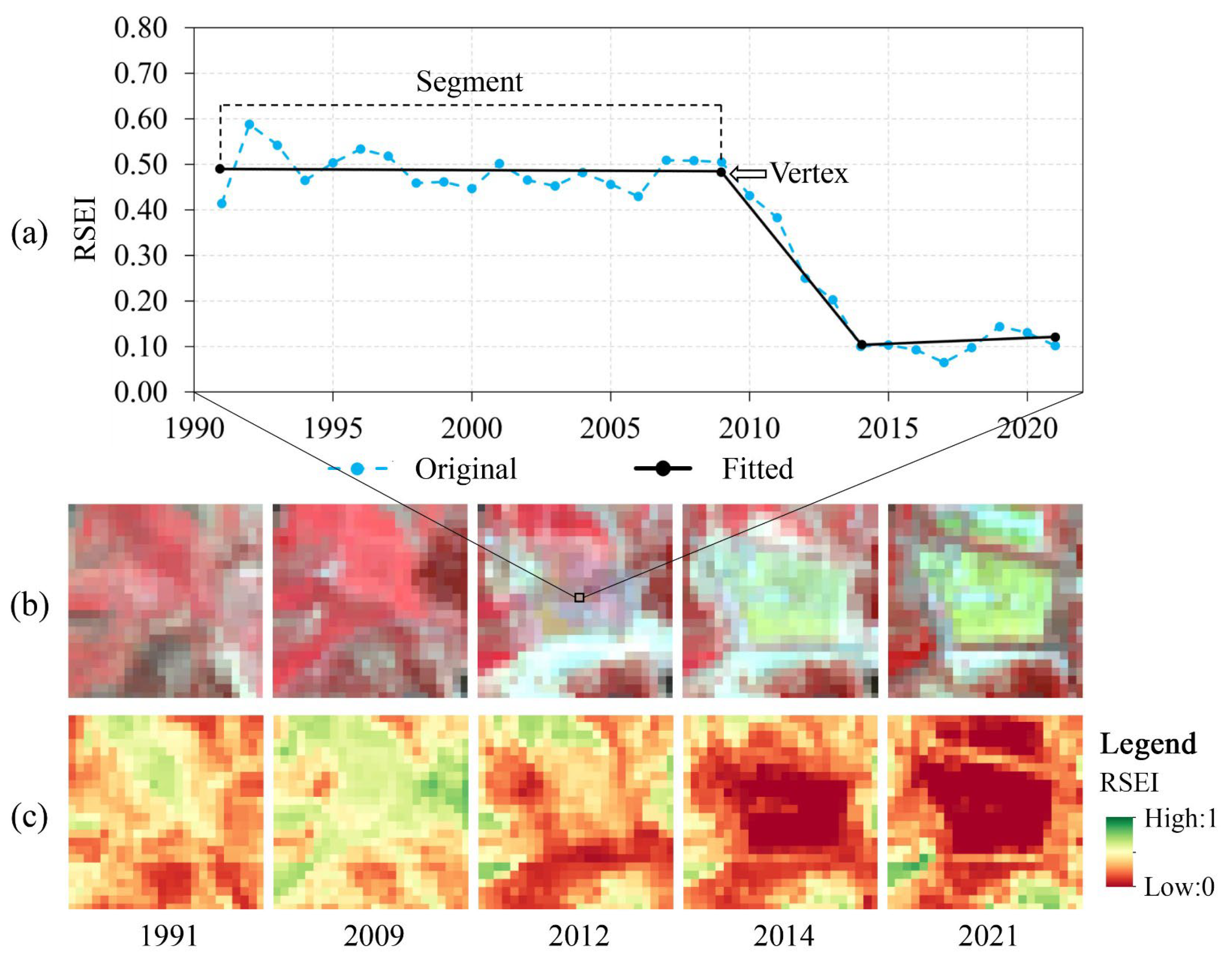
2.3.2. Spatial–Temporal Change Detection Algorithm of RSEI

The LandTrendr (Landsat-based detection of Trends in Disturbance and Recovery) algorithm was applied to analyze and better understand the spatial and temporal EQ changes on a pixel basis [40]. LandTrendr is a time series segmentation algorithm that divides the time series data into multiple segments and can detect abrupt and gradual changes by comparing the relevant results (Figure 3). In addition, LandTrendr eliminates the noise from the time series and describes the temporal, spectral trajectories more clearly [40]. In this study, LandTrendr was used to detect the RSEI disturbance, representing the process from the higher value of RSEI to the lower value. Detected changes of RSEI contained the start time, end time, and duration of the disturbance.

The LandTrendr algorithm can be divided into five parameter sets based on the parameter functions: (1) controls for the detection time range, (2) inputs for the spectral band or index, (3) controls for the trajectory segment performance, (4) orientation of the vegetation change tendency, and (5) options for pixel filtering [50]. Under the same detection time range and RSEI change tendency, Max segments, Recovery threshold, and Best model proportion in the controls for the trajectory segment performance are the key parameters that affect the accuracy of LandTrendr [6]. Max segments can identify breakpoints in the RSEI series. The recovery threshold can filter out the short-duration time segments that are shorter than the user-defined threshold. The best model proportion is used to control the fitting of the trajectory and overfitting. Therefore, Max segments, Recovery threshold, and Best model proportion were selected and determined in this study.

In order to evaluate the accuracy of LandTrendr for detecting RSEI disturbance, the results of RSEI disturbance were verified by obtaining 189 temporal samples using the stratified random sampling strategy. Sample collection was based on Landsat images and would significantly reduce the first occurrence time of ecological environment quality degradation, including forest disturbance and the conversion of forest area and cultivated land to built-up land.

The detected change was considered to be correct when the time detected by the LandTrender algorithm and the actual time of temporal samples was less than 3 years. The ratio of correct disturbance and the number of temporal samples represents the detection accuracy of the LandTrendr algorithm [50]. It was found that the highest accuracy of 91.01% was achieved when the values of Max segments, Recovery threshold, and Best model proportion were 5, 0.3, and 0.5, respectively (

Table 2. List of LandTrendr parameters.

Parameter	Values
Max segments	4
	5
	6
Recovery threshold	0.3
	0.5
	0.7
Best model proportion	0.5
	1
	1.25

Note: Numbers in bold represent parameters with the highest accuracy.

).

3. Results

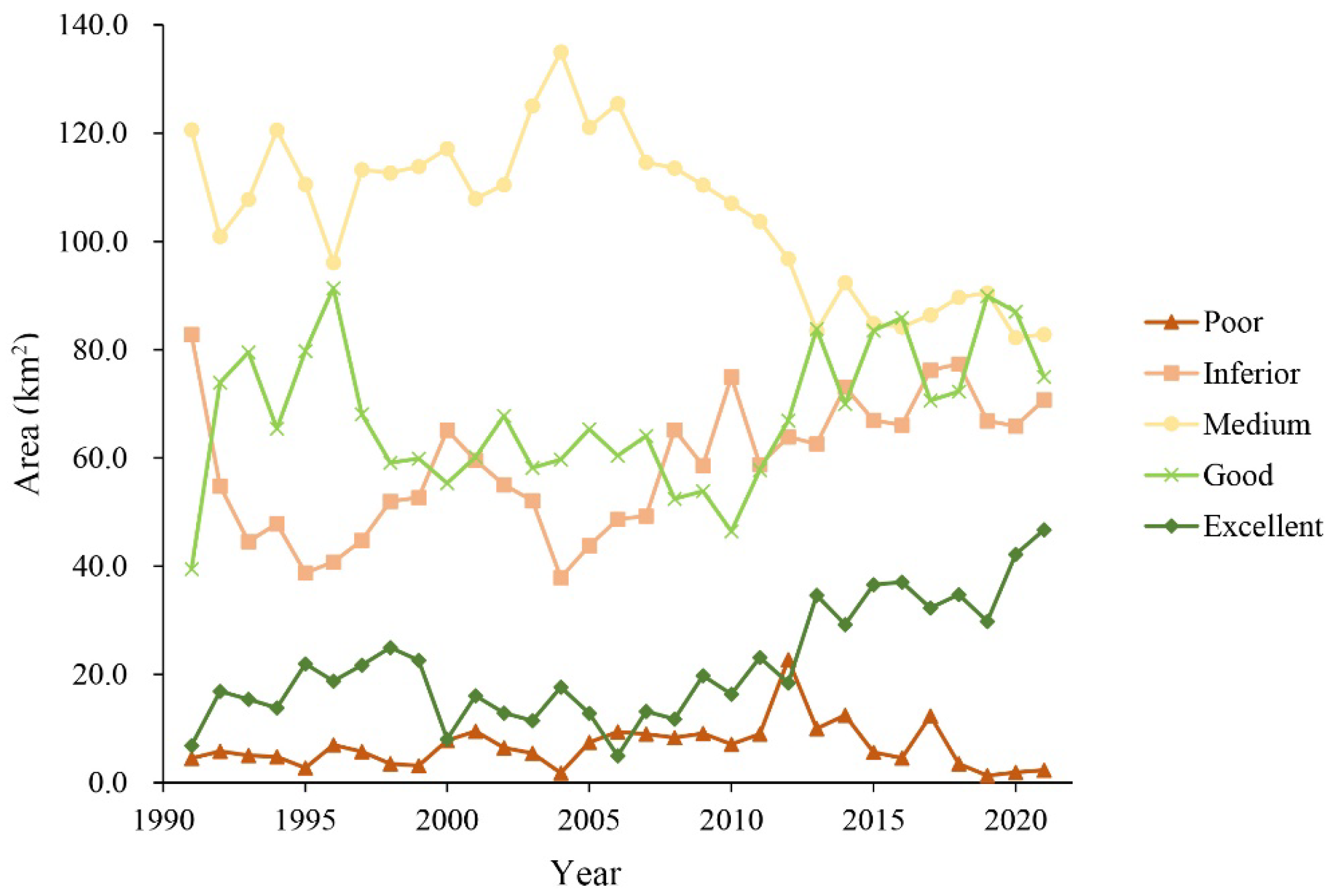
3.1. Quantitative Assessment of Ecological Quality (EQ) from 1991 to 2021

The result of PC1 is shown in the Supplementary Data (Table S1). The NDVI and Wet indices had positive effects on EQ, while NDISI and LST indices had negative effects. The effects of the NDVI and NDISI indices had more obvious importance than Wet and LST for Haitan Island. Moreover, the highest PC1 explained 88.05% of the total variation of four metrics, and the lowest PC1 explained 78.30% of the total variation between 1991 and 2021. This indicates that the composed RSEI from PC1 was able to express the EQ on Haitan Island. Therefore, RSEIs from 1991 to 2021 were calculated based on the PC1, and the average value of RSEI was 0.53 over 31 years, with the highest RSEI value in 2020 (0.57) and the lowest RSEI value in 1991 (0.47). Figure 4 presents examples of the spatial and temporal distribution of RSEI.

The areas of RSEI at different levels are shown in Figure 5. It can be seen that the medium level for RSEI had the largest area over 31 years, reaching an average of 105.19 km², followed by the good level (67.83 km²) and inferior level (58.62 km²). The excellent and poor levels had the lowest area, reaching an average of 21.69 km² and 6.74 km². Notably, the RSEI for the poor level had the highest area in 2012 compared to the other years.

3.2. Cumulative Analysis of Ecological Quality (EQ) from 1991 to 2021 at Each Level

To better understand the EQ of Haitan Island over 31 years, the statistics of pixel-based RSEI at each level are shown in Figure 6. It can be seen that the different levels of RSEI had visible patterns; that is, the poor level mainly occurred on sandy beaches and in urban areas (Figure 6a); the medium level of EQ mainly occurred in cultivated land and mountainous areas with a small amount visible in forest areas (Figure 6c); the good level of EQ was mainly distributed in the areas with relatively high forest and vegetation coverage (Figure 6d); the distribution of excellent EQ was located on the northeast and southwest of the island in the forested mountain area (Figure 6e).

The cumulative tally of the different levels of EQ is presented in Table 3. It can be seen that 47.87 km² of the island was affected by a poor EQ at least once in 31 years. Within this area, 36.26 km² had poor EQ between one and five times, which represents up to 12.78% of the island’s total area. A total of 235.91 km² had no poor EQ rating over time, representing 83.13% of the island’s total area. An area of 198.03 km² (83.13%) of the island had been impacted by an inferior EQ at least once, with 91.65 km² being affected between one and five times and 44.97 km² having inferior EQ between six and ten times over 31 years. Up to 236.30 km² (83.27%) of the island had medium EQ at least once during the study period. There was a total of 199.76 km² affected by a good EQ at least once. A total of 209.96 km² had no excellent EQ rating, and only 73.83 km² had an excellent EQ at least once in 31 years.

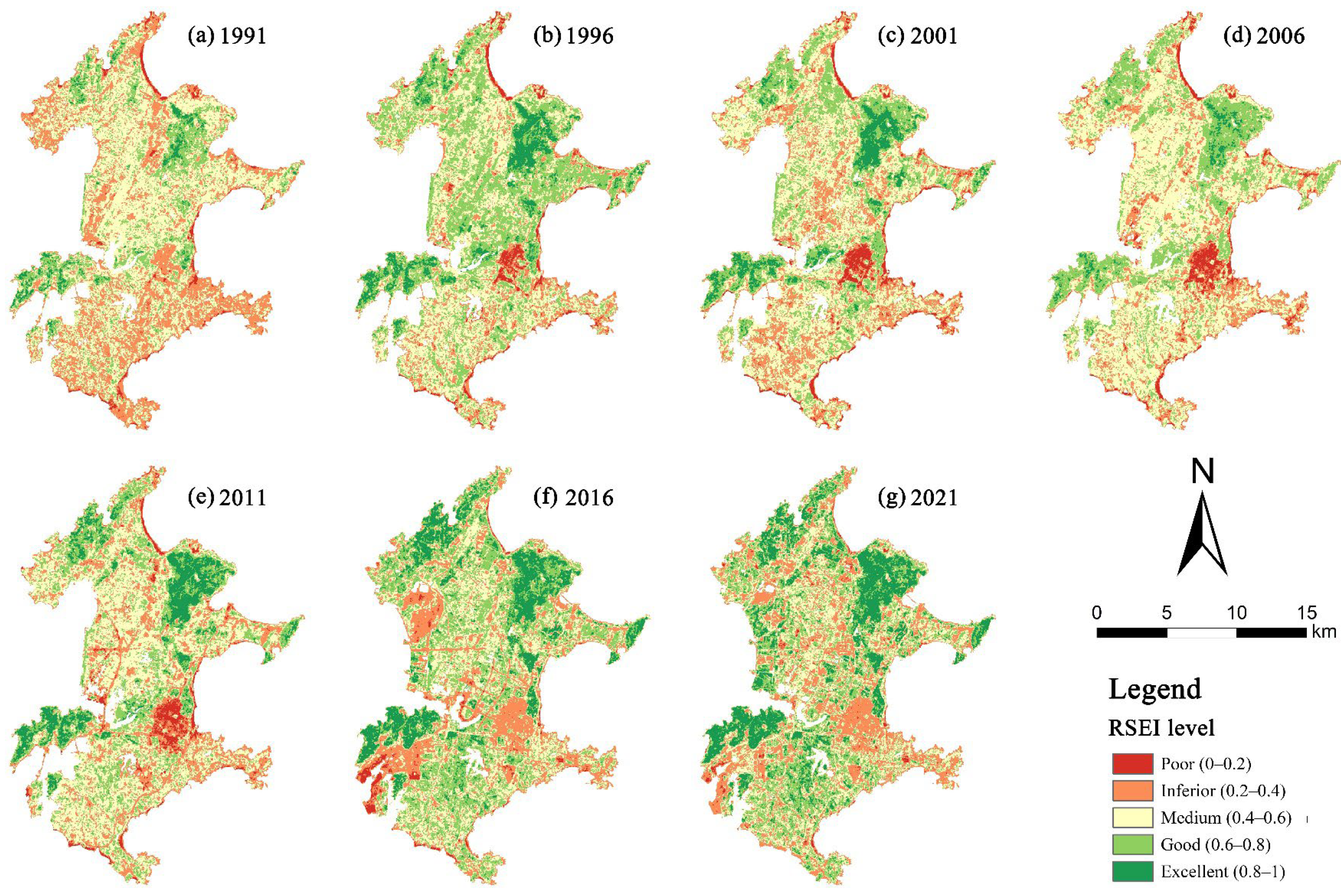
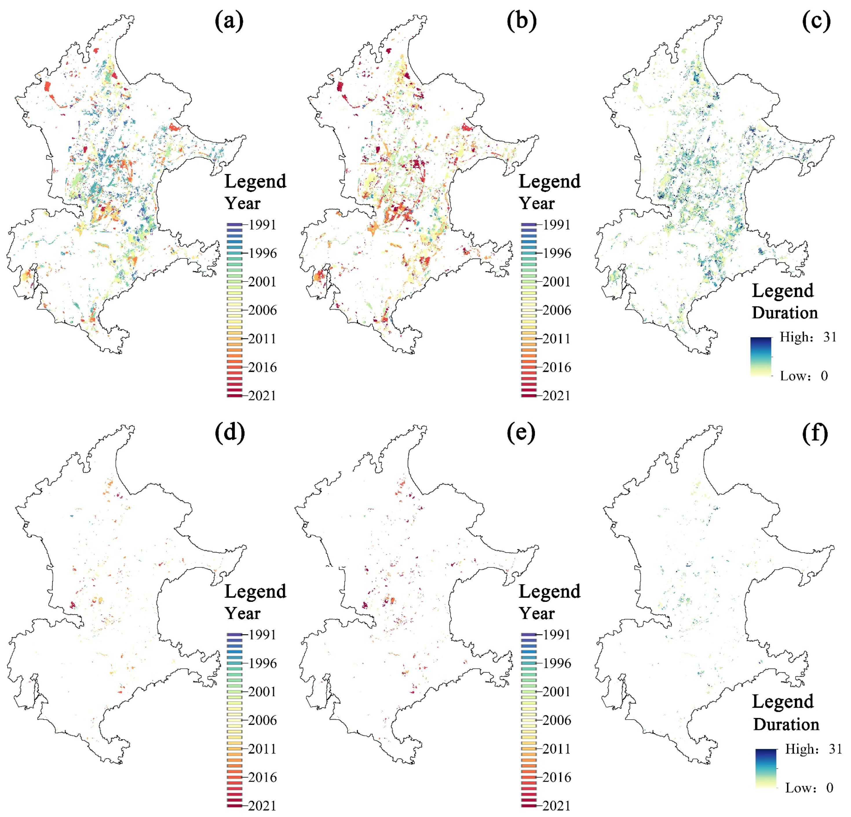
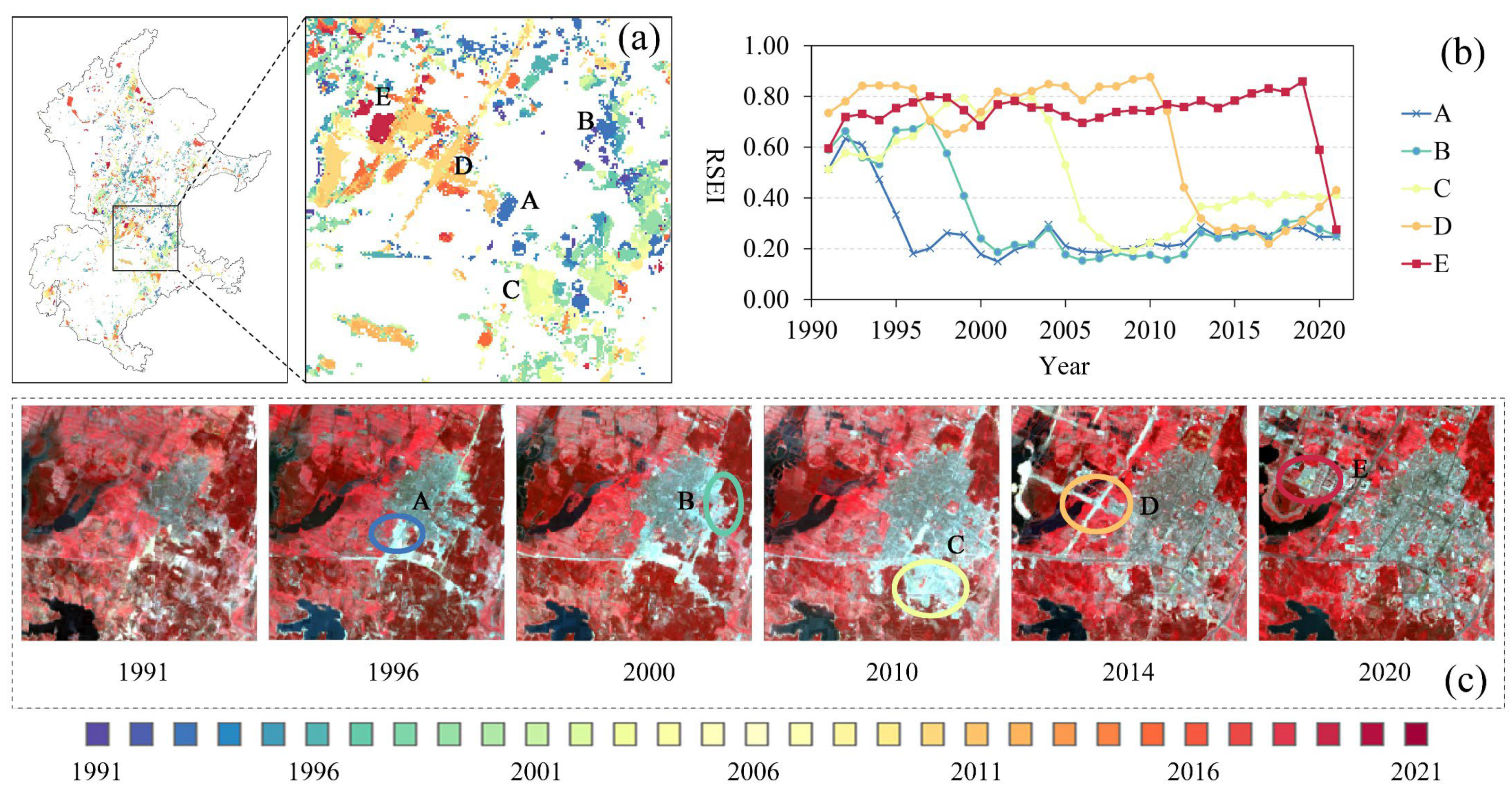
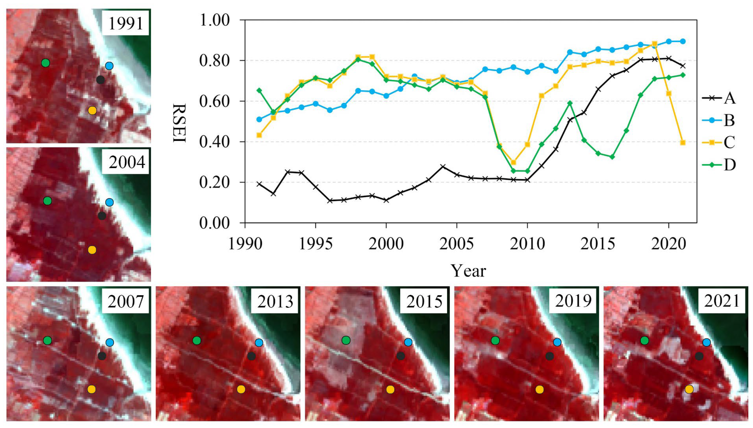
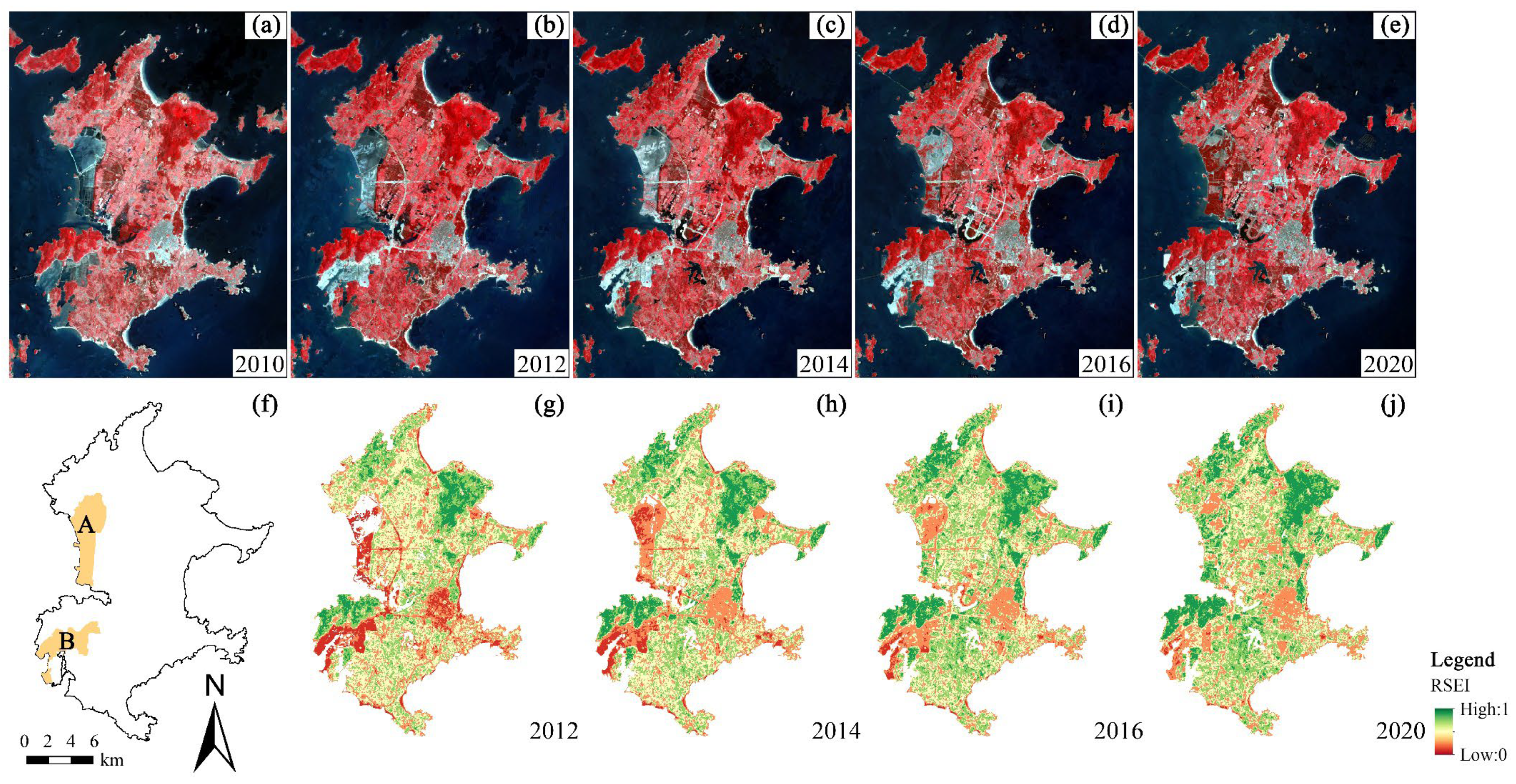
3.3. Spatial–Temporal Analysis of Ecological Quality (EQ) Changes

Figure 7 shows the results of spatial–temporal RSEI changes on a pixel basis using the LandTrendr algorithm, including the disturbance start time, end time, and duration. As seen from

Table 4. Area statistics of ecological quality (EQ) disturbance in 31 years.

Year	Areas of Initial Disturbance			Areas of Ending Disturbance
	First Disturbance/km2	Second Disturbance/km2	Cumulative Sum	First Disturbance/km2	Second Disturbance/km2	Cumulative Sum
1991	1.34	-	1.34	-	-	-
1992	0.02	-	0.02	0.27	-	0.27
1993	3.19	-	3.19	0.16	-	0.16
1994	0.53	-	0.53	0.24	-	0.24
1995	1.20	0.05	1.25	0.05	-	0.05
1996	4.62	0.02	4.64	0.41	-	0.41
1997	1.13	0.02	1.14	0.39	-	0.39
1998	1.74	0.03	1.78	0.97	0.02	0.98
1999	2.39	0.04	2.44	0.94	0.01	0.96
2000	0.41	0.01	0.42	1.51	0.02	1.53
2001	1.56	0.05	1.61	3.46	0.01	3.47
2002	2.15	0.10	2.24	1.34	0.02	1.36
2003	0.44	0.01	0.45	1.64	0.01	1.65
2004	2.40	0.10	2.50	0.52	0.01	0.52
2005	1.12	0.13	1.25	1.34	0.03	1.36
2006	0.67	0.12	0.79	2.11	0.05	2.16
2007	1.10	0.13	1.23	1.64	0.02	1.66
2008	0.35	0.07	0.42	1.87	0.06	1.93
2009	1.82	0.16	1.98	1.28	0.04	1.32
2010	1.38	0.11	1.49	1.79	0.09	1.88
2011	0.59	0.15	0.74	0.85	0.05	0.90
2012	0.55	0.14	0.69	3.05	0.22	3.27
2013	2.04	0.57	2.61	0.94	0.08	1.03
2014	0.75	0.12	0.87	1.27	0.19	1.47
2015	1.31	0.22	1.54	0.68	0.21	0.89
2016	1.60	0.25	1.85	0.74	0.23	0.97
2017	0.59	0.07	0.66	2.55	0.38	2.93
2018	0.41	0.07	0.48	1.33	0.24	1.57
2019	0.72	0.19	0.91	0.98	0.10	1.07
2020	0.12	0.09	0.21	0.09	0.01	0.10
2021	-	-	0.00	3.83	0.95	4.77
Total	38.22	3.05	41.27	34.40	2.10	41.27

, a total of 41.27 km² of cumulative disturbance area occurred in the past 31 years. Within this area, 38.22 km² of EQ disturbance occurred from 1991 to 2021, accounting for 13.77% of the island area in 2021, and 3.05 km² of EQ disturbance area occurred twice. The year with the largest initial disturbance area was 1996, with an increase of 4.64 km² in newly disturbed area. The year with the largest ending disturbance area was 2001 (up to 3.47 km²). In 2021, there was still 4.77 km² of disturbed area identified. In general, the average time of disturbance was 5.69 years (Figure 7c,f), with 62.2% of the area under disturbance for five years or less, accounting for 25.67 km² of area. The area subject to constant disturbance for three years represented the largest area with up to 23.92% (9.87 km²) of the island. A total of 4.57 km² had constant disturbance for ten years or more, impacting 11.08% of the island.

Figure 6. Cumulative number of times for ecological quality (EQ) at different levels over 31 years. (a): poor; (b): inferior; (c): medium; (d): good; (e): excellent.

Figure 6. Cumulative number of times for ecological quality (EQ) at different levels over 31 years. (a): poor; (b): inferior; (c): medium; (d): good; (e): excellent.

Table 3. Area statistics of cumulative value of ecological quality (EQ) at different levels in 31 years.

Cumulative Number of Times	Poor/km2	Inferior/km2	Medium/km2	Good/km2	Excellent/km2
0	235.91	85.77	47.49	84.04	209.96
1–5	36.26	91.65	55.21	63.96	36.13
6–10	6.25	44.97	33.11	49.22	13.89
11–15	2.81	19.99	37.68	34.65	7.63
16–20	1.50	14.56	50.61	27.05	5.13
21–25	0.71	11.36	41.84	17.56	4.43
26–31	0.34	15.50	17.85	7.32	6.61

Table 3. Area statistics of cumulative value of ecological quality (EQ) at different levels in 31 years.

Cumulative Number of Times	Poor/km2	Inferior/km2	Medium/km2	Good/km2	Excellent/km2
0	235.91	85.77	47.49	84.04	209.96
1–5	36.26	91.65	55.21	63.96	36.13
6–10	6.25	44.97	33.11	49.22	13.89
11–15	2.81	19.99	37.68	34.65	7.63
16–20	1.50	14.56	50.61	27.05	5.13
21–25	0.71	11.36	41.84	17.56	4.43
26–31	0.34	15.50	17.85	7.32	6.61

4. Discussion

4.1. Ecological Quality (EQ) Changes

In terms of the four metrics considered, it is evident that higher vegetation coverage, soil-plant moisture, lower temperature, and land surface dryness contribute to a better EQ. The average RSEI values in the past 31 years were between 0.47 and 0.53, which indicated the overall EQ of Haitan Island was at a medium level. Although the original EQ of Haitan Island was fragile, the RSEI values maintained a stable level from 1991 to 2021. This implies that anthropogenic activities have double-sided impacts on the ecological environment. Coastal shelter forest planting, urban greening, ecological agriculture, and other measures improve the EQ. In contrast, tourism development, road construction, and other construction make the EQ face greater pressure and decrease the level of RSEI. For each RSEI level on the island, different countermeasures should be taken to maintain or improve the EQ. For instance, proper land use planning is necessary to control the intensity of construction and increase the use of green infrastructure in areas with poor and inferior RSEI levels. The area with excellent and good RSEI levels mainly belongs to forest areas where human disturbance should be prohibited or avoided, particularly in coastal and mountainous regions. For the areas with a medium RSEI level, it is necessary to protect the soil and avoid large amounts of cultivated land being occupied by built-up land during urban expansion.

4.2. Effects of Urban Expansion on Ecological Quality (EQ)

Land cover change (LCC) caused by urban expansion is the key factor associated with EQ fluctuations. Similar to Haitan Island, other coastal islands have also experienced urban expansion in China [51,52]. Moreover, previous studies have reported urban expansion is also the main reason for ecosystem services to change [3]. In our previous study, we reported that built-up land increased by 16.20% from 1990 to 2019, with much of the cultivated land being converted to built-up land on Haitan Island [53]. During the period of urban expansion, other land use types (e.g., cultivated land, forest, grassland) were converted into barren land first, then transformed into built-up land. Therefore, the value of RSEI declined sharply in a short time (Figure 8) and then slowly recovered to a stable level due to green infrastructure being developed in the built-up land.

4.3. Effects of Forest Change on Ecological Quality (EQ)

Although a policy of afforestation has been implemented on the island and barren land has been converted to forest over the past 31 years, this study found that RSEI decreased in some forest areas (Figure 9). The forest degradation may be explained by the clearing of some coastal forests. The RSEI can reflect forest change, including forest deforestation and forest degradation caused by natural disasters. As seen in Figure 9, the location of C may be explained by diseases that lead to forest death, resulting in the degradation of EQ. Forest deforestation can result in approximately 25% of the net CO₂ emissions from forests [54,55]. It is critical to detect forest degradation in its initial stages to support sustainable forest management. Therefore, monitoring RSEI changes can identify forest disturbance, such as the location and severity of a pest attack and the potential drivers of pest prediction [56,57,58,59].

4.4. Effects of Policies on Ecological Quality (EQ)

Policy is another factor that has impacted the EQ change. In China, rapid economic development and government policies have accelerated land use change. Haitan Island has a special geographic location, which connects the Pacific Ocean and Taiwan Strait, and plays an important role in southeast trade routes. The ‘Comprehensive Pilot Zone’ program accelerated the development of Haitan Island [3]. It can be seen that the medium RSEI level gradually decreased in 2011 because of cultivated land reduction and built-up land expansion (Figure 5). Notably, the five levels of RSEI on Haitan Island fluctuated significantly with the increase in human activities between 2010 and 2015, particularly in the middle and western regions.

As seen in Figure 10, the implementation and progress of reclamation projects has occurred. It was found that the area of poor RSEI level increased from 8.96 km² to 22.74 km² between 2011 and 2012 because of land reclamation. Because of different policy orientations, afforestation was carried out in area A and a port and trade zone was developed in area B (Figure 10). The level of RSEI improved rapidly with the growth of afforestation in area A. While the RSEI in area B was maintained at a low level due to land construction, the RSEI gradually improved to an inferior and medium level until 2018. This can be explained by the gradually developing green infrastructure, which was reflected in an improved RSEI level.

In addition, the strategies of the ‘Grain for Green Project’ and ‘Coastal shelter forests planting’ have been implemented on Haitan Island, which has played a critical role in preventing wind erosion. Thus, by positioning Haitan Island as an international tourism island, a reasonable policy-making decision would be essential for the future of the ecological environment of Haitan Island.

4.5. Advantages and Disvantages of RSEI

The RSEI integrates multi-dimensional surface ecological information, which can help us better understand the interactions between anthropogenic activities and natural ecology. Compared to other evaluation methods, RSEI has the advantages of easily obtained parameters, the ability for time series analysis, and a wide evaluation range. Through this study’s review of previous studies, we demonstrated that using RSEI is feasible to monitor the EQ changes of Haitan Island. A previous study reported that the RSEI values for Haitan Island in 2007, 2011, 2014, and 2017 were 0.519, 0.506, 0.502, and 0.523, respectively [26]. Although these results are similar to our study (0.519, 0.521, 0.520, 0.522 in 2007, 2011, 2014, and 2017, respectively), this earlier study is unable to represent the EQ in a given year because only one scene was used per year for this analysis [26]. In our study, the annual composed image was able to represent the RSEI of the corresponding year more accurately because it avoided the vegetation coverage changes caused by seasonal variations that can affect the calculation of RSEI.

The RSEI has become a widely used comprehensive remote sensing ecological environment index, although some previous studies proposed to detect time series ecological change using an improved comprehensive remote sensing ecological index (IRSEI) [60] or a discrete RSEI (DRSEIs) [8]. They suggested improving the RSEI by using the z-score standardized RSEI [8] and the entropy weight method and PCA [60], which mainly considers the instability of RSEI in its application and the insufficient information utilization by PCA. That discussion is of great interest to the topic and helps to promote the RSEI application. It is important to note that RSEI can analyze and predict the changes of EQ from the two aspects of space and time with non-subjective intervention, and its derivation from remote sensing images completely. In general, the existing RSEI proposed by Xu et al. [24] is an effective and stable tool to some extent.

4.6. Limitations and Future Prospects

Cloud coverage often occurs in the study area, which is a limitation in obtaining the available images. Moreover, the requirement of temporal remote sensing data confines the algorithm application. It is challenging to obtain monthly images of Haitan Island. Previous studies proposed combining optical remote sensing imagery (e.g., Sentinel data, Landsat data) for monitoring EQ. For instance, Landsat and Sentinel-2 images were combined to capture the rapid permafrost disturbance in the high northern latitudes of Siberia [6]. Cardille et al. fused Landsat-8 and Sentinel-2A and -2B data to detect forest disturbance [61]. Therefore, using multi-sensors for time series EQ assessments should be studied further. Even though the Landsat missions are designed for continuity, there is sensor bias across the different Landsat missions [62,63,64]. For our study, these sensor biases are much smaller than the differences in vegetation phenology caused by acquisition date differences and are mitigated by the Landtrendr algorithm, which serves to eliminate noise in the time series data.

5. Conclusions

Increasing human activities bring greater pressure to the ecological environment. Rapidly and effectively monitoring EQ can help better understand the human impact on the ecological environment. Haitan Island is one of the islands with accelerated urbanization in China. In this study, the change of EQ in timing and location from the spatial–temporal patterns of Haitan Island over the past 31 years was explored. The time series Landsat imagery from 1991 to 2021 was selected and composited in the GEE platform to calculate the annual RSEI on Haitan Island. The LandTrendr algorithm was adopted to achieve a relatively complete analysis of EQ changes. This study provides a reference for continuous ecological environment monitoring and can contribute information for policymakers as they plan for the future.

The results showed that the average value of RSEI was between 0.47 and 0.57 over the past 31 years (1991–2021) on the island, and the medium RSEI level had the most extensive area (105.19 km²). The inferior and poor RSEI level was mainly located in the middle and western regions of the island. A total of 41.27 km² experienced cumulative disturbance within the island. Disturbance primarily occurred in the main urban area, development zone, and some forested regions. The primary reason for disturbance in the main urban area and the development zone was the removal of original vegetation during the construction process, and the built-up area being maintained as bare land for part of this process.

References

1. Jupiter, S.; Mangubhai, S.; Kingsford, R.T. Conservation of biodiversity in the pacific islands of Oceania: Challenges and opportunities. Pac. Conserv. Biol. 2014, 20, 206. [Google Scholar] [CrossRef]
2. Rombouts, I.; Beaugrand, G.; Artigas, L.F.; Dauvin, J.C.; Gevaert, F.; Goberville, E.; Kopp, D.; Lefebvre, S.; Luczak, C.; Spilmont, N.; et al. Evaluating marine ecosystem health: Case studies of indicators using direct observations and modelling methods. Ecol. Indic. 2013, 24, 353–365. [Google Scholar] [CrossRef]
3. Shifaw, E.; Sha, J.; Li, X.; Bao, Z.; Zhou, Z. An insight into land-cover changes and their impacts on ecosystem services before and after the implementation of a comprehensive experimental zone plan in Pingtan island, China. Land Use Pol. 2019, 82, 631–642. [Google Scholar] [CrossRef]
4. Sun, D.Q.; Zhang, J.X.; Zhu, C.G.; Hu, Y.; Zhou, L. An assessment of China’s ecological environment quality change and its spatial variation. Acta Geogr. Sin. 2012, 67, 1599–1610. [Google Scholar]
5. Wu, H.Y.; Chen, K.L.; Chen, Z.H.; Chen, Q.H.; Qiu, Y.P.; Wu, J.C.; Zhang, J.F. Evaluation for the ecological quality status of coastal waters in East China Sea using fuzzy integrated assessment method. Mar. Pollut. Bull. 2012, 64, 546–555. [Google Scholar] [PubMed]
6. Runge, A.; Nitze, I.; Grosse, G. Remote sensing annual dynamics of rapid permafrost thaw disturbances with LandTrendr. Remote Sens. Environ. 2022, 268, 112752. [Google Scholar] [CrossRef]
7. Shan, W.; Jin, X.; Ren, J.; Wang, Y.; Xu, Z.; Fan, Y.; Gu, Z.; Hong, C.; Lin, J.; Zhou, Y. Ecological environment quality assessment based on remote sensing data for land consolidation. J. Clean. Prod. 2019, 239, 118126. [Google Scholar] [CrossRef]
8. Zheng, Z.; Wu, Z.; Chen, Y.; Guo, C.; Marinello, F. Instability of remote sensing based ecological index (RSEI) and its improvement for time series analysis. Sci. Total Environ. 2022, 814, 152595. [Google Scholar]
9. Xiong, Y.; Xu, W.; Lu, N.; Huang, S.; Wu, C.; Wang, L.; Dai, F.; Kou, W. Assessment of spatial-temporal changes of ecological environment quality based on RSEI and GEE: A case study in Erhai Lake Basin, Yunnan province, China. Ecol. Indic. 2021, 125, 107518. [Google Scholar] [CrossRef]
10. Wang, C.; Jiang, Q.; Shao, Y.; Sun, S.; Xiao, L.; Guo, J. Ecological environment assessment based on land use simulation: A case study in the Heihe River Basin. Sci. Total Environ. 2019, 697, 133928. [Google Scholar] [CrossRef]
11. Li, Y.; Cao, Z.; Long, H.; Liu, Y.; Li, W. Dynamic analysis of ecological environment combined with land cover and NDVI changes and implications for sustainable urban–rural development: The case of Mu Us Sandy Land, China. J. Clean. Prod. 2017, 142, 697–715. [Google Scholar] [CrossRef]
12. Wu, S.; Chen, Y. Examining eco-environmental changes at major recreational sites in Kenting National Park in Taiwan by integrating SPOT satellite images and NDVI. Tour. Manag. 2016, 57, 23–36. [Google Scholar] [CrossRef]
13. Liang, S.; Yi, Q.; Liu, J. Vegetation dynamics and responses to recent climate change in Xinjiang using leaf area index as an indicator. Ecol. Indic. 2015, 58, 64–76. [Google Scholar]
14. Wang, Q.; Tenhunen, J.; Dinh, N.; Reichstein, M.; Otieno, D.; Granier, A.; Pilegarrd, K. Evaluation of seasonal variation of MODIS derived leaf area index at two European deciduous broadleaf forest sites. Remote Sens. Environ. 2005, 96, 475–484. [Google Scholar]
15. Wang, X.D.; Zhong, X.H.; Liu, S.Z.; Liu, J.G.; Wang, Z.Y.; Li, M.H. Regional assessment of environmental vulnerability in the Tibetan Plateau: Development and application of a new method. J. Arid Environ. 2008, 72, 1929–1939. [Google Scholar] [CrossRef]
16. Ivits, E.; Cherlet, M.; Mehl, W.; Sommer, S. Estimating the ecological status and change of riparian zones in Andalusia assessed by multi-temporal AVHHR datasets. Ecol. Indic. 2009, 9, 422–431. [Google Scholar]
17. Asadi Zarch, M.A.; Malekinezhad, H.; Mobin, M.H.; Dastorani, M.T.; Kousari, M.R. Drought monitoring by Reconnaissance Drought Index (RDI) in Iran. Water Resour. Manag. 2011, 25, 3485–3504. [Google Scholar] [CrossRef] [Green Version]
18. Naresh Kumar, M.; Murthy, C.S.; Sesha Sai, M.V.R.; Roy, P.S. On the use of Standardized Precipitation Index (SPI) for drought intensity assessment. Meteorol. Appl. 2009, 16, 381–389. [Google Scholar] [CrossRef] [Green Version]
19. Rhee, J.; Im, J.; Carbone, G.J. Monitoring agricultural drought for arid and humid regions using multi-sensor remote sensing data. Remote Sens. Environ. 2010, 114, 2875–2887. [Google Scholar]
20. Mildrexler, D.J.; Zhao, M.; Running, S.W. Testing a MODIS Global Disturbance Index across North America. Remote Sens. Environ. 2009, 113, 2103–2117. [Google Scholar] [CrossRef]
21. Yang, X.; Meng, F.; Fu, P.; Wang, Y.; Liu, Y. Time-frequency optimization of RSEI: A case study of Yangtze River Basin. Ecol. Indic. 2022, 141, 109080. [Google Scholar] [CrossRef]
22. Yang, X.; Meng, F.; Fu, P.; Zhang, Y.; Liu, Y. Spatiotemporal change and driving factors of the Eco-Environment quality in the Yangtze River Basin from 2001 to 2019. Ecol. Indic. 2021, 131, 108214. [Google Scholar] [CrossRef]
23. Cui, R.; Han, J.; Hu, Z. Assessment of spatial temporal changes of ecological environment quality: A case study in Huaibei City, China. Land 2022, 11, 944. [Google Scholar] [CrossRef]
24. Xu, H.Q. A remote sensing index for assessment of regional ecological changes. China Environ. Sci. 2013, 33, 889–897. [Google Scholar]
25. Liu, C.; Yang, M.; Hou, Y.; Zhao, Y.; Xue, X. Spatiotemporal evolution of island ecological quality under different urban densities: A comparative analysis of Xiamen and Kinmen Islands, southeast China. Ecol. Indic. 2021, 124, 107438. [Google Scholar]
26. Wen, X.; Ming, Y.; Gao, Y.; Hu, X. Dynamic monitoring and analysis of ecological quality of Pingtan Comprehensive Experimental Zone, a new type of sea island city, based on RSEI. Sustainability 2020, 12, 21. [Google Scholar] [CrossRef] [Green Version]
27. Yuan, B.; Fu, L.; Zou, Y.; Zhang, S.; Chen, X.; Li, F.; Deng, Z.; Xie, Y. Spatiotemporal change detection of ecological quality and the associated affecting factors in Dongting Lake Basin, based on RSEI. J. Clean. Prod. 2021, 302, 126995. [Google Scholar]
28. Gao, W.; Zhang, S.; Rao, X.; Lin, X.; Li, R. Landsat TM/OLI-Based Ecological and Environmental Quality Survey of Yellow River Basin, Inner Mongolia Section. Remote Sens. 2021, 13, 4477. [Google Scholar]
29. Xu, H.; Wang, M.; Shi, T.; Guan, H.; Fang, C.; Lin, Z. Prediction of ecological effects of potential population and impervious surface increases using a remote sensing based ecological index (RSEI). Ecol. Indic. 2018, 93, 730–740. [Google Scholar]
30. DeVries, B.; Verbesselt, J.; Kooistra, L.; Herold, M. Robust monitoring of small-scale forest disturbances in a tropical montane forest using Landsat time series. Remote Sens. Environ. 2015, 161, 107–121. [Google Scholar]
31. Tamiminia, H.; Salehi, B.; Mahdianpari, M.; Quackenbush, L.; Adeli, S.; Brisco, B. Google Earth Engine for geo-big data applications: A meta-analysis and systematic review. ISPRS—J. Photogramm. Remote Sens. 2020, 164, 152–170. [Google Scholar] [CrossRef]
32. Wang, L.; Diao, C.; Xian, G.; Yin, D.; Lu, Y.; Zou, S.; Erickson, T.A. A summary of the special issue on remote sensing of land change science with Google Earth Engine. Remote Sens. Environ. 2020, 248, 112002. [Google Scholar]
33. Gorelick, N.; Hancher, M.; Dixon, M.; Ilyushchenko, S.; Thau, D.; Moore, R. Google Earth Engine: Planetary-scale geospatial analysis for everyone. Remote Sens. Environ. 2017, 202, 18–27. [Google Scholar] [CrossRef]
34. Dewi, R.; Bijker, W.; Stein, A. Change vector analysis to monitor the changes in fuzzy shorelines. Remote Sens. 2017, 9, 147. [Google Scholar] [CrossRef] [Green Version]
35. Xian, G.; Homer, C.; Fry, J. Updating the 2001 National Land Cover Database land cover classification to 2006 by using Landsat imagery change detection methods. Remote Sens. Environ. 2009, 113, 1133–1147. [Google Scholar]
36. Yu, W.; Zhou, W.; Qian, Y.; Yan, J. A new approach for land cover classification and change analysis: Integrating backdating and an object-based method. Remote Sens. Environ. 2016, 177, 37–47. [Google Scholar]
37. Zhu, Z.; Woodcock, C.E. Continuous change detection and classification of land cover using all available Landsat data. Remote Sens. Environ. 2014, 144, 152–171. [Google Scholar] [CrossRef] [Green Version]
38. Brooks, E.B.; Wynne, R.H.; Thomas, V.A.; Blinn, C.E.; Coulston, J.W. On-the-Fly massively multitemporal change detection using statistical quality control charts and Landsat data. IEEE Trans. Geosci. Remote Sens. 2014, 52, 3316–3332. [Google Scholar]
39. Vogelmann, J.E.; Gallant, A.L.; Shi, H.; Zhu, Z. Perspectives on monitoring gradual change across the continuity of Landsat sensors using time-series data. Remote Sens. Environ. 2016, 185, 258–270. [Google Scholar]
40. Kennedy, R.E.; Yang, Z.; Cohen, W.B. Detecting trends in forest disturbance and recovery using yearly Landsat time series: 1. LandTrendr—Temporal segmentation algorithms. Remote Sens. Environ. 2010, 114, 2897–2910. [Google Scholar] [CrossRef]
41. de Jong, S.M.; Shen, Y.; de Vries, J.; Bijnaar, G.; van Maanen, B.; Augustinus, P.; Verweij, P. Mapping mangrove dynamics and colonization patterns at the Suriname coast using historic satellite data and the LandTrendr algorithm. Int. J. Appl. Earth Obs. Geoinf. 2021, 97, 102293. [Google Scholar]
42. Fu, B.; Lan, F.; Xie, S.; Liu, M.; He, H.; Li, Y.; Liu, L.; Huang, L.; Fan, D.; Gao, E.; et al. Spatio-temporal coupling coordination analysis between marsh vegetation and hydrology change from 1985 to 2019 using LandTrendr algorithm and Google Earth Engine. Ecol. Indic. 2022, 137, 108763. [Google Scholar] [CrossRef]
43. Huang, H.; Chen, Y.; Clinton, N.; Wang, J.; Wang, X.; Liu, C.; Gong, P.; Yang, J.; Bai, Y.; Zheng, Y.; et al. Mapping major land cover dynamics in Beijing using all Landsat images in Google Earth Engine. Remote Sens. Environ. 2017, 202, 166–176. [Google Scholar] [CrossRef]
44. Zhu, Z.; Woodcock, C.E. Object-based cloud and cloud shadow detection in Landsat imagery. Remote Sens. Environ. 2012, 118, 83–94. [Google Scholar]
45. Zhu, Z.; Wang, S.; Woodcock, C.E. Improvement and expansion of the Fmask algorithm: Cloud, cloud shadow, and snow detection for Landsats 4–7, 8, and Sentinel 2 images. Remote Sens. Environ. 2015, 159, 269–277. [Google Scholar]
46. Cohen, W.B.; Yang, Z.; Healey, S.P.; Kennedy, R.E.; Gorelick, N. A LandTrendr multispectral ensemble for forest disturbance detection. Remote Sens. Environ. 2018, 205, 131–140. [Google Scholar]
47. Flood, N. Seasonal composite Landsat TM/ETM+ images using the Medoid (A multi-dimensional median). Remote Sens. 2013, 5, 6481–6500. [Google Scholar]
48. Robinson, N.; Allred, B.; Jones, M.; Moreno, A.; Kimball, J.; Naugle, D.; Erickson, T.; Richardson, A. A dynamic Landsat derived Normalized Difference Vegetation Index (NDVI) product for the conterminous united states. Remote Sens. 2017, 9, 863. [Google Scholar]
49. Xu, H.Q. A study on information extraction of water body with the modified normalized difference water index (MNDWI). J. Remote Sens. 2005, 9, 589–595. [Google Scholar]
50. Xu, H.; Wei, Y.; Liu, C.; Li, X.; Fang, H. A scheme for the long-term monitoring of impervious—Relevant land disturbances using high frequency Landsat archives and the Google Earth Engine. Remote Sens. 2019, 11, 1891. [Google Scholar]
51. Cao, H.; Liu, J.; Fu, C.; Zhang, W.; Wang, G.; Yang, G.; Luo, L. Urban expansion and its impact on the land use pattern in Xishuangbanna since the reform and opening up of China. Remote Sens. 2017, 9, 137. [Google Scholar] [CrossRef] [Green Version]
52. Lin, T.; Xue, X.; Shi, L.; Gao, L. Urban spatial expansion and its impacts on island ecosystem services and landscape pattern: A case study of the island city of Xiamen, Southeast China. Ocean. Coast. Manag. 2013, 81, 90–96. [Google Scholar]
53. Lin, L.; Hao, Z.; Post, C.J.; Mikhailova, E.A.; Yu, K.; Yang, L.; Liu, J. Monitoring land cover change on a rapidly urbanizing island using Google Earth Engine. Appl. Sci. 2020, 10, 7336. [Google Scholar] [CrossRef]
54. Federici, S.; Tubiello, F.N.; Salvatore, M.; Jacobs, H.; Schmidhuber, J. New estimates of CO2 forest emissions and removals: 1990–2015. For. Ecol. Manag. 2015, 352, 89–98. [Google Scholar] [CrossRef] [Green Version]
55. Baccini, A.; Walker, W.; Carvalho, L.; Farina, M.; Sulla-Menashe, D.; Houghton, R.A. Tropical forests are a net carbon source based on aboveground measurements of gain and loss. Science 2017, 358, 230–234. [Google Scholar] [CrossRef] [Green Version]
56. Campbell, M.J.; Dennison, P.E.; Tune, J.W.; Kannenberg, S.A.; Kerr, K.L.; Codding, B.F.; Anderegg, W.R.L. A multi-sensor, multi-scale approach to mapping tree mortality in woodland ecosystems. Remote Sens. Environ. 2020, 245, 111853. [Google Scholar]
57. Gomez Selvaraj, M.; Vergara, A.; Montenegro, F.; Alonso Ruiz, H.; Safari, N.; Raymaekers, D.; Ocimati, W.; Ntamwira, J.; Tits, L.; Omondi, A.B.; et al. Detection of banana plants and their major diseases through aerial images and machine learning methods: A case study in DR Congo and Republic of Benin. ISPRS–J. Photogramm. Remote Sens. 2020, 169, 110–124. [Google Scholar] [CrossRef]
58. Meng, R.; Gao, R.; Zhao, F.; Huang, C.; Sun, R.; Lv, Z.; Huang, Z. Landsat-based monitoring of southern pine beetle infestation severity and severity change in a temperate mixed forest. Remote Sens. Environ. 2022, 269, 112847. [Google Scholar]
59. Yu, R.; Luo, Y.; Zhou, Q.; Zhang, X.; Wu, D.; Ren, L. A machine learning algorithm to detect pine wilt disease using UAV-based hyperspectral imagery and LiDAR data at the tree level. Int. J. Appl. Earth Obs. Geoinf. 2021, 101, 102363. [Google Scholar] [CrossRef]
60. Li, J.; Gong, J.; Guldmann, J.; Yang, J. Assessment of urban ecological quality and spatial heterogeneity based on remote sensing: A case study of the rapid urbanization of Wuhan city. Remote Sens. 2021, 13, 4440. [Google Scholar] [CrossRef]
61. Cardille, J.A.; Perez, E.; Crowley, M.A.; Wulder, M.A.; White, J.C.; Hermosilla, T. Multi-sensor change detection for within-year capture and labelling of forest disturbance. Remote Sens. Environ. 2022, 268, 112741. [Google Scholar]
62. Claverie, M.; Vermote, E.F.; Franch, B.; Masek, J.G. Evaluation of the Landsat-5 TM and Landsat-7 ETM+ surface reflectance products. Remote Sens. Environ. 2015, 169, 390–403. [Google Scholar] [CrossRef]
63. Ke, Y.; Im, J.; Lee, J.; Gong, H.; Ryu, Y. Characteristics of Landsat 8 OLI-derived NDVI by comparison with multiple satellite sensors and in-situ observations. Remote Sens. Environ. 2015, 164, 298–313. [Google Scholar]
64. Che, X.; Zhang, H.K.; Liu, J. Making Landsat 5, 7 and 8 reflectance consistent using MODIS nadir-BRDF adjusted reflectance as reference. Remote Sens. Environ. 2021, 262, 112517. [Google Scholar]
Figure 2. The collected Landsat imagery for Haitan Island by day of year (DOY) from 1991 to 2021.
Remotesensing 14 05773 g002
Figure 3. Example of LandTrendr’s segmentation and fitting of time series remote sensing-based ecological index (RSEI). (a) a line chart with the selected point, original RSEI values, and corresponding fitted values; (b) example of land cover type change at corresponding positions in Landsat images; (c) example of RSEI change in corresponding years.
Remotesensing 14 05773 g003
Figure 4. Example of five-leveled remote sensing-based ecological index (RSEI) images of Haitan Island. The different boundaries are due to reclamation. (a) RSEI in 1991; (b) RSEI in 1996; (c) RSEI in 2001; (d) RSEI in 2006; (e) RSEI in 2011; (f) RSEI in 2016; (g) RSEI in 2021.
Remotesensing 14 05773 g004
Figure 5. Area statistics of remote sensing-based ecological index (RSEI) at different levels from 1991 to 2021. The area of RSEI in Figure 4 is without water.
Remotesensing 14 05773 g005
Figure 7. Spatial–temporal distribution of ecological quality (EQ) disturbance in Haitan Island from 1991 to 2021. Different colors represent different years. (a): start time of the first disturbance; (b): end time of the first disturbance; (c): duration of the first disturbance; (d): start time of the second disturbance; (e): end time of the second disturbance; (f): duration of the second disturbance.
Remotesensing 14 05773 g007
Figure 8. Impact of land use change on remote sensing-based ecological index (RSEI) (1991–2021) for Haitan Island. (a): enlarged example of the start time of the disturbance; (b): changes of RSEI in five regions; (c): example of Landsat images.
Remotesensing 14 05773 g008
Figure 9. Analysis of RSEI changes in forest area.
Remotesensing 14 05773 g009
Figure 10. Analysis of remote sensing-based ecological index (RSEI) changes in reclamation. (ae) Landsat images, shown in near-infrared, red, and green; (f) locations of A and B reclamation areas; (gj) RSEI in 2012, 2014, 2016, and 2020, respectively.
Remotesensing 14 05773 g010