Article

Assimilation of Water Vapor Retrieved from Radar Reflectivity Data through the Bayesian Method

1
Institute of Desert Meteorology, China Meteorological Administration, Urumqi 830002, China
2
National Observation and Research Station of Desert Meteorology, Taklimakan Desert of Xinjiang, Urumqi 830002, China
3
Taklimakan Desert Meteorology Field Experiment Station of CMA, Urumqi 830002, China
4
Xinjiang Key Laboratory of Desert Meteorology and Sandstorm, Urumqi 830002, China
5
Key Laboratory of Tree-Ring Physical and Chemical Research, China Meteorological Administration, Urumqi 830002, China
6
Institute of Urban Meteorology, China Meteorological Administration, Beijing 100089, China
*
Author to whom correspondence should be addressed.
Remote Sens. 2022, 14(22), 5897; https://0-doi-org.brum.beds.ac.uk/10.3390/rs14225897
Submission received: 3 October 2022 / Revised: 8 November 2022 / Accepted: 15 November 2022 / Published: 21 November 2022

Abstract

:
This work describes the implementation of an updated radar reflectivity assimilation scheme with the three-dimensional variational (3D-Var) system of Weather Research and Forecast (WRF). The updated scheme, instead of the original scheme assuming the relative humidity to a fixed value where radar reflectivity is higher than a threshold, assimilates pseudo water vapor retrieved by the Bayesian method, which would be consistent with clouds/precipitations provided by the model in theory. To verify the effect of the updated scheme to the improvement of precipitation simulation, a convective case in Wenquan County and the continuous monthly simulation with contrasting experiments in Xinjiang were performed. The test of single reflectivity observation demonstrates that the water vapor retrieved by the Bayesian method is consistent with the meteorological situation around. In the convective case, both the updated and original scheme results show that the assimilation of pseudo water vapor can adjust to the environmental conditions of water vapor and temperature. This can improve the hourly precipitation forecast skill more than the contrasting experiment, which was designed to only assimilate conventional observations and radar radial velocity data. In the continuous monthly experiments, the updated scheme reveals that the analysis of water vapor is more reasonable, and obtains a better precipitation forecast skill for 6 h accumulated precipitation than the contrasting experiments.

1. Introduction

Uncertainties of weather forecasts are mostly due to inaccuracies in initial conditions and shortcomings of physics in the models of numerical weather prediction (NWP). The former plays the most significant role in resolving convection, and representing clouds and precipitation reasonably. Radar data is particularly well suited to convective-scale data assimilation (DA) because it provides high resolutions of temporal and spatial data, which are in general higher than the conventional observations; it also contains hydrometeor and dynamical information [1,2,3,4].
Advances in data assimilation techniques including complex cloud analysis [5,6,7], three-dimensional or four-dimensional variational data assimilation (3D-Var or 4D-Var) [8,9,10,11,12], the ensemble Kalman filter (EnKF), hybrid variational using ensemble approaches [13,14,15], and the assimilation of radar data including reflectivity and radial velocity have been extensively used in convective-scale NWP models. The observations of radar radial velocity contain dynamical information which is an important component of the atmospheric wind field. The observations of radar reflectivity provide various kinds of hydrometeor information. However, many challenges for the assimilation of radar data still exist because the radial velocity and reflectivity cannot directly be predicted by NWP models [8,10,11]. The transform relationships between radar reflectivity and hydrometeor variables are generally nonlinear [16].
In complex cloud analysis schemes, the hydrometeor and thermodynamic variables are tuned up based on surface observations, radar and satellite data, etc. [17], which can alleviate the spin-up problem of precipitation forecast quite effectively [5,18]. However, typically empirical relationships are widely used in complex cloud analysis algorithms in which many uncertainties need to be dealt with. Moreover, background and observation error information, which can give statistically optimal estimations, are also not to be fully utilized in complex cloud analysis schemes. The phenomenon of overpredicting precipitation often occurs when the complex cloud analysis schemes are used in cycled data assimilation, especially in radar reflectivity assimilation [5].
Within variational framework, the prognostic variables from models including rainwater, snow, crystal and graupel, etc., are necessary to be transformed into the observed reflectivity. The Z–R relationship based on Marshall–Palmer distribution of raindrop size was used to perform the transformation in early studies [1,9,19]; it was developed for warm cloud precipitation. To improve this deficiency of limited application, several further studies, which involve snow and graupel in the observation operator of reflectivity assimilation, effectively improve the hydrometeor analysis, and can be applied to the cold-cloud process [8,20]. For the convective-scale NWP models, the complex microphysical processes are especially important. The direct observation operator involves physical processes which are characterized by discontinuities and nonlinearities, and there is need of simplification in the linearized versions to get some good results [21]. In the existing 4D-Var systems, radar reflectivity assimilation assumes that the microphysics for warm rain appear first and then transform reflectivity to a rainwater mixing ratio [1,11]. However, the minimization convergence of assimilation becomes a nonnegligible problem, since the cost function’s gradient of the reflectivity observation term would be abnormally large. Since the rainwater mixing ratio in the background is actually quite small, the analysis error of rainwater is extremely large [4,11,18].
The studies above mentioned have confirmed that the scheme of direct radar reflectivity can improve the initial conditions for the convective-scale weather and also can benefit the subsequent forecasts. However, one problem is the direct assimilation method depends on empirical algorithms to transform the hydrometeor variables, which were usually developed for S-band radar or a certain area, and in which many uncertain parameters require tuning up. Another problem is caused by the linearization of the tangent linear (TL) operator and adjoint (AD) operator [8,9].
In the variational method, assimilating the reflectivity-retrieved hydrometeor profiles is a common indirect approach that became involved to avoid the problem of linearization of the TL/AD operators. Additionally, some studies found that the assimilation of humidity profiles has a larger impact on the precipitation forecasts compared to hydrometeor profiles assimilation [18]. A set of simulation experiments using an observing system test found that water vapor and horizontal wind observations have the greatest contribution to short-range forecasts and storm-scale analyses among all types of measurements [22]. Water vapor has great influence on radiation transfer and the thermodynamic structure of the entire atmosphere [23,24,25]. Water vapor assimilation can effectively improve the simulation of convection intensity and updraft height by enhancing the content and vertical distribution of water vapor [26]. Realizing the important role of water vapor assimilation in convective-scale precipitation forecasts, many studies have focused on using different indirect assimilation methods to assimilate radar reflectivity, such as pseudo relative humidity, and water vapor observations retrieved. Wang et al. (2013) developed pseudo relative humidity and water vapor retrieved with WRF 3D-Var and successfully promoted the development of the convective system [10]. Caumont et al. (2010) developed a one-dimensional (1D) approach to assimilate volumes of radar reflectivity data used in the Arome model at Meteo-France [27,28].
In this paper, the 3D-Var method is chosen for the reason that it has a significantly lower computational burden than the more advanced 4D-Var, EnKF, and hybrid methods. An updated scheme of indirect radar reflectivity assimilation is implemented into the framework of the WRF-DA system, which assimilates water vapor profiles retrieved through the Bayesian method. This is referring to Caumont et al. (2010), and based on the original scheme developed by Wang et al. (2013) [10,27,28]. The original scheme, which assumes the relative humidity to a fixed value where radar reflectivity is higher than a threshold, does not take the background hydrometeor information into consideration.
The rest of this paper is organized as follows. In Section 2, the water vapor retrieval and radar reflectivity assimilation algorithm are introduced. In Section 3, to verify the effect for the updated scheme, a convective case on 30 July 2019 in Wenquan County and the continuous monthly experiments from 1 July to 31 July 2019 in Xinjiang are designed. Section 4 presents the analysis and forecast results with contrasting experiments. Finally, a summary and conclusions are given in Section 5.

2. Methodology

The sequence of operations of water vapor retrieval and assimilation methods are illustrated in Figure 1. The first step is to retrieve vertical profiles of pseudo relative humidity from the vertical profiles of observed and simulated reflectivity. The second step is the retrieval of vertical profiles of pseudo water vapor using the observation operator of reflectivity assimilation [10]. The third step consists of assimilating the pseudo water vapor with the WRF 3D-Var system which was built during the second step.

2.1. Water Vapor Retrieval

The water vapor is retrieved by the observation operator from Equation (8) below, in which the saturated specific humidity can be obtained from the model background. The relative humidity retrieval uses the Bayesian method, which assumes that the simulated profiles occur with almost the same relative frequency from a large database as those found in the region or in nature [29,30]. In the following, the Bayesian method is briefly recalled [27,28], and how the water vapor retrieval is applied to this study is presented.
In Equation (1), the best estimate of X given the set of observations Y o is
E ( X ) = X × P ( X = X t r u e | Y = Y o ) d X
where X is the model state vector of a vertical profile to retrieve, X t r u e is the true state vector, and the vector Y o is a set of available observations. Based on Bayes’ theorem [31], Equation (1) could be rewritten as Equation (2),
E ( X ) = X × P ( Y = Y o | X = X t r u e ) P ( X = X t r u e ) d X
In this case, let us assume that the errors are Gaussian and uncorrelated in the observed and simulated observations. Equation (2) could be rewritten as Equation (3),
P ( Y = Y o | X = X t r u e ) exp [ 1 2 ( Y o H ( X ) ) T R 1 ( Y o H ( X ) ) ]
where R represents the error covariance matrices of observation and simulation, and H represents the observation operator which can simulate observations from the NWP model. Using this assumption which was mentioned before, Equation (2) can be approximated by Equation (4),
E ( X ) = i X i ω i j ω j
with Equation (5),
ω i = exp [ 1 2 ( Y o H ( X i ) ) T R 1 ( Y o H ( X i ) ) ]
where ω i is the weight of a model profile, and subscript i represents the index of a model profile in the vicinity of the observed profile of reflectivity.
The observed reflectivity from the plan position indicator (PPI) planes can be interpolated to a Cartesian grid in different elevation. The observations in a column can be treated as a vertical profile. For each vertical profile of observed reflectivity ( Y Z ), a vertical profile of pseudo relative humidity observations Y p o r h is expressed as Equation (6),
Y p o r h = i X i r h ω i j ω j
with Equation (7),
ω i = exp [ 1 2 ( Y Z H Z ( X i ) ) T R Z 1 ( Y Z H Z ( X i ) ) ]
where X i are the columns of model background state, a square window of 21 × 21 columns, in the vicinity of Y Z , X i r h are the corresponding vertical profiles of model relative humidity interpolated at each observation elevation, H Z ( X i ) are the corresponding vertical profiles of simulated reflectivity, and R Z is the observation and simulation error covariance matrices of reflectivity, which is chosen as a diagonal term equal to 0.2 n dBZ, where n is the number of observations in a vertical profile [27,28].
A vertical profile of pseudo water vapor observations, Y p o q v is calculated by the observation operator H with Equation (8), which was developed by Wang et al. (2013) in the WRF-DA system [10],
Y p o q v = Y p o r h × X q s
where X q s are the corresponding vertical profiles of model saturated specific humidity interpolated at each observation elevation.

2.2. Radar Reflectivity Assimilation

Each vertical profile of pseudo water vapor is assimilated, as any other observations, with the WRF-DA system [32]. In 3D-Var method, the following cost function J ( X ) with Equation (9), is minimized for a state vector X that represents all model variables at all grid points,
J ( X ) = 1 2 ( X X b ) T B 1 ( X X b ) + 1 2 [ Y H ( X ) ] T R 1 [ Y H ( X ) ] T
where X b represents the background state vector, the observation operator H of water vapor is consistent with Equation (8) before, and B represents the background error covariance matrix. The statistics of background error covariance were calculated by the National Meteorological Center (NMC) method [33], using pairs of the differences between the 12 and 24 h forecasts. There were 31 day forecasts from 1 July to 31 July 2019 used to generate the B with U and V as the part of control variables.
The gradient of cost function is calculated for its minimization as follows, Equation (10),
J X = B 1 ( X X b ) H T R 1 [ Y H ( X ) ]
with the necessary condition J X = 0 , J ( X ) to be a minimum. In Equation (11),
X a = X b + [ B 1 + H T R 1 H 1 ] 1
where X a is the analysis state vector. Superscript T represents the process of matrix transposition. The observation operator H T , through the simplification process, is mainly affected by water vapor and temperature. When a positive increment of water vapor is assimilated, positive increments of temperature will also be obtained [10].

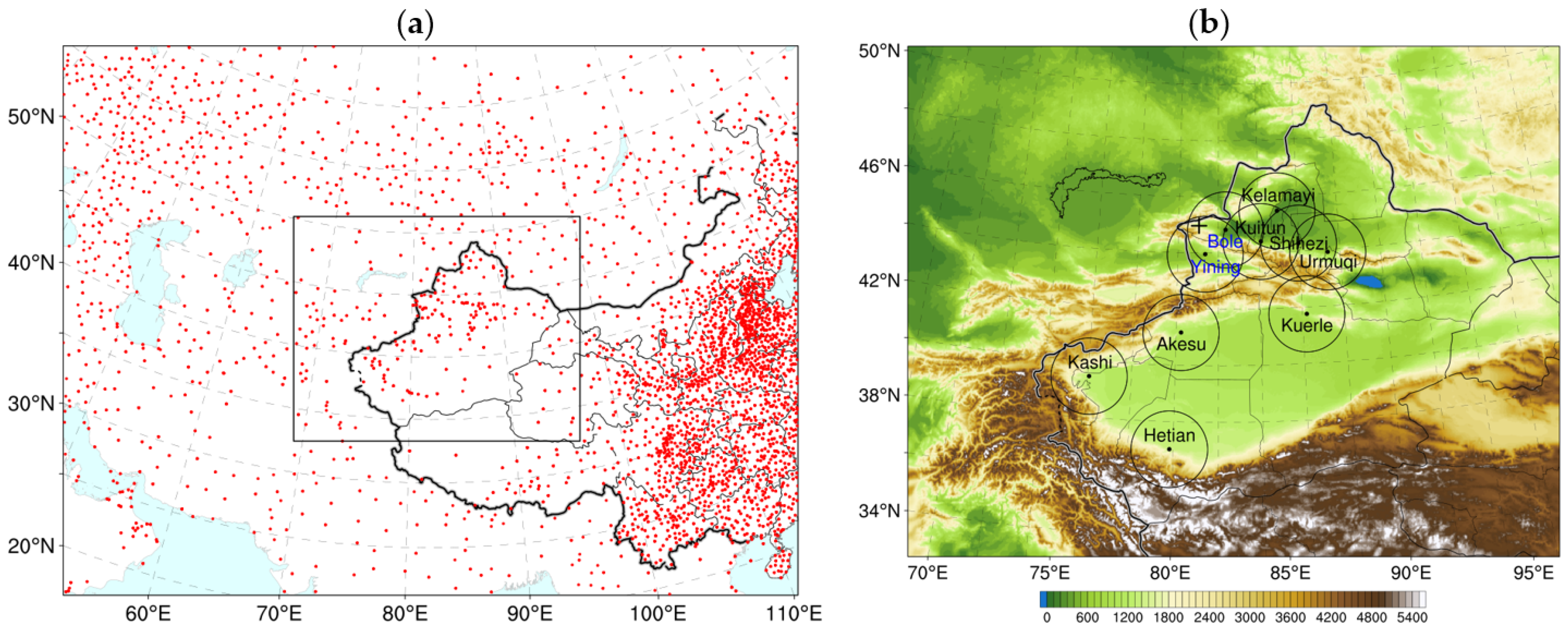
3. Model and Experimental Design

3.1. Model Configuration

The Advanced Research WRF model and WRF-DA system in version 3.9.1 [34,35] were used for deterministic numerical weather forecasting. The fundamental configuration of WRF is listed in Table 1. Two nested domains were built in the mode. Domain 1 covered most of the Central Asia region, with a grid spacing of 9 km and 712 × 532 grid points. Domain 2 was centered on Xinjiang, China, with a grid spacing of 3 km and 832 × 652 grid points (Figure 1). A total of 50 vertical computational layers were used with the pressure maximum of 10 hPa. Atmospheric and surface fields from the final operational global analysis data from the Global Forecasting System of National Centers for Environment Prediction (NCEP-FNL) were introduced as the initial and lateral boundary conditions which are collected at 6 h intervals and a horizontal resolution of 0.25° × 0.25° [36]. The physics schemes included WSM6 microphysics, the shortwave and longwave scheme of RRTMG, the Unified Noah land-surface model, Kain–Fritsch deep convection, and ACM2 PBL in domain 1 [37,38,39,40,41]. Domain 2 uses the same physical parameterization configuration described here except for no parameterization of deep convection.

3.2. Data Used for Assimilation and Validation

Conventional observation data of specific synoptic hours (SYNOP) from global surface weather stations are shown as the red dots in Figure 2a, assimilated in domain 1 and domain 2. In addition to conventional data, reflectivity and radial velocity from C-band Doppler radar data were also assimilated at a different step, in which an analysis obtained by assimilating SYNOP is used as a background in domain 2 in Figure 2b. Both hourly data assimilated from conventional observations and radar are obtained from the National Meteorological Information Center [42].
The pre-processing and quality control of radar data include clutter removal, data thinning of 10 km resolution, and so on. In Figure 2b, radar data of Bole and Yining are used for the convective case in Wenquan County. All nine Doppler station’s radar data are used for continuous monthly experiments in Xinjiang. Hourly and 6 h accumulated precipitation from SYNOP are taken for verifying the forecast skill in convective case and continuous monthly experiments, respectively. Before the calculation of forecast skill score, the accumulated precipitation at the model grid points was interpolated near the observation stations of SYNOP. The interpolation method is a weighted sum of values in the interpolation area of 5 × 5 grids nearest the observation station, in which the weight given to each model grid point is the reciprocal of the square of the distance.

3.3. Experimental Design

To determine the impact of pseudo water vapor assimilated by the 3D-VAR method, a convective case and continuous experiments were performed. A convective case, a moderate-to-heavy precipitation event was selected: 30 July 2019 over the central and northeastern part of Wenquan County (Figure 2b) in which the main precipitation periods were at 0900 UTC. For the convective case study selected, Figure 3a shows the flowchart of the cycled data assimilation and forecast. The model is cold started at 0000 UTC, and runs through 6 h (noted as the ‘spin up’) to reach equilibrium at the simulation initial condition, then the data assimilation is cycled at 1 h intervals from 0600 to 0800 UTC. The forecasts are launched every hour. The flowchart of continuous monthly experiments is shown in Figure 3b, in which the main precipitation periods were concentrated between 1200 and 1800 UTC. The model is cold started at 0600 UTC, then runs spin up for 6 h, then assimilates observations and forecasts for 6 h.
For the convective case (continuous experiments), data from 2 Doppler radars overlapped in the simulation domain (Figure 2b). Three groups of experiments were performed. The contrasting runs, labeled as C1Con and E1Con, respectively, assimilated radar radial velocity and surface conventional observations from SYNOP. Experiments of C2Rad and E2Rad were the same as the contrasting experiments, but added the assimilation of pseudo water vapor retrieved by reflectivity based on the original scheme. In this, the relative humidity retrieved depended on empirical values of different observed reflectivity ranges. For example, the relative humidity is assumed to be 85%, at which the observed radar reflectivity is higher than 25 dBZ and lower than 45 dBZ above cloud base [10]. The original scheme does not take the background hydrometeor information into account. Experiments of C3RadBy and E3RadBy were the same as C2Rad and E2Rad but different in the relative humidity retrieval using the Bayesian method. The details of each experiment are shown in Table 2.

4. Result

4.1. Test of Single Reflectivity Observation

Before the experiments were conducted, the test of a single reflectivity observation is performed to verify the response of relative humidity retrieval. The model’s first guess is interpolated from the global analysis data of NCEP-FNL at 0800 UTC 30 July 2019 [36]. The single reflectivity observation of 35.9 dBZ is assumed at 44.91°N, 80.95°E, 12th model level, approximately 3000 m. The 21 × 21 grid points centered on the point of single reflectivity observation were used to retrieve relative humidity (Figure 4a,b). Figure 4c shows the weight of each neighbouring grid point. It is expected that, the smaller the differences between simulated and observed reflectivity, the larger the weight is [27,28]. Figure 4e shows that the relative humidity retrieved is a linear combination of neighbouring grids taken from the simulated relative humidity. The relative humidity retrieved at the single reflectivity observation point by the updated scheme is set to 95.8% (Figure 4e) and is set to 85% based on the original scheme (Figure 4f), where simulated relative humidity is 78%. The result of relative humidity retrieved was more consistent with the model meteorological situation around in the updated scheme than the original scheme [22,28].

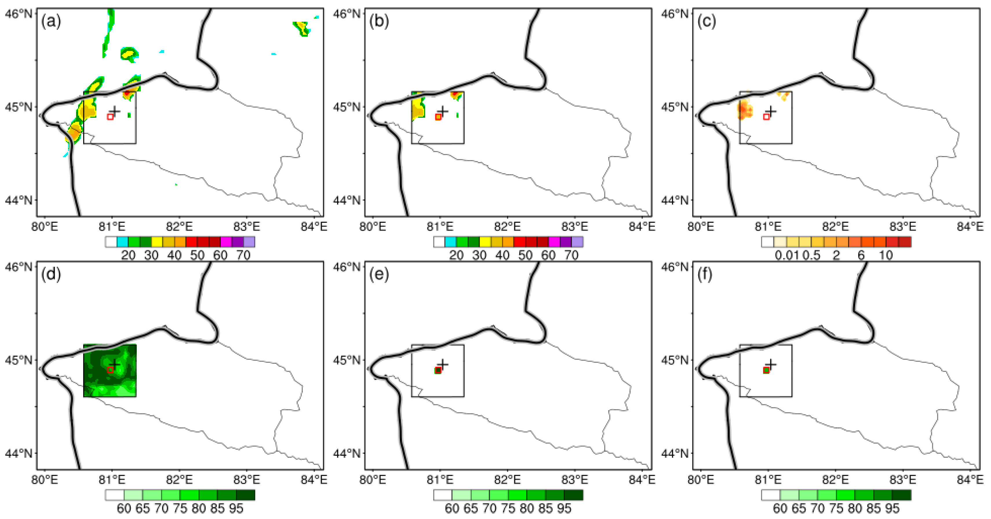
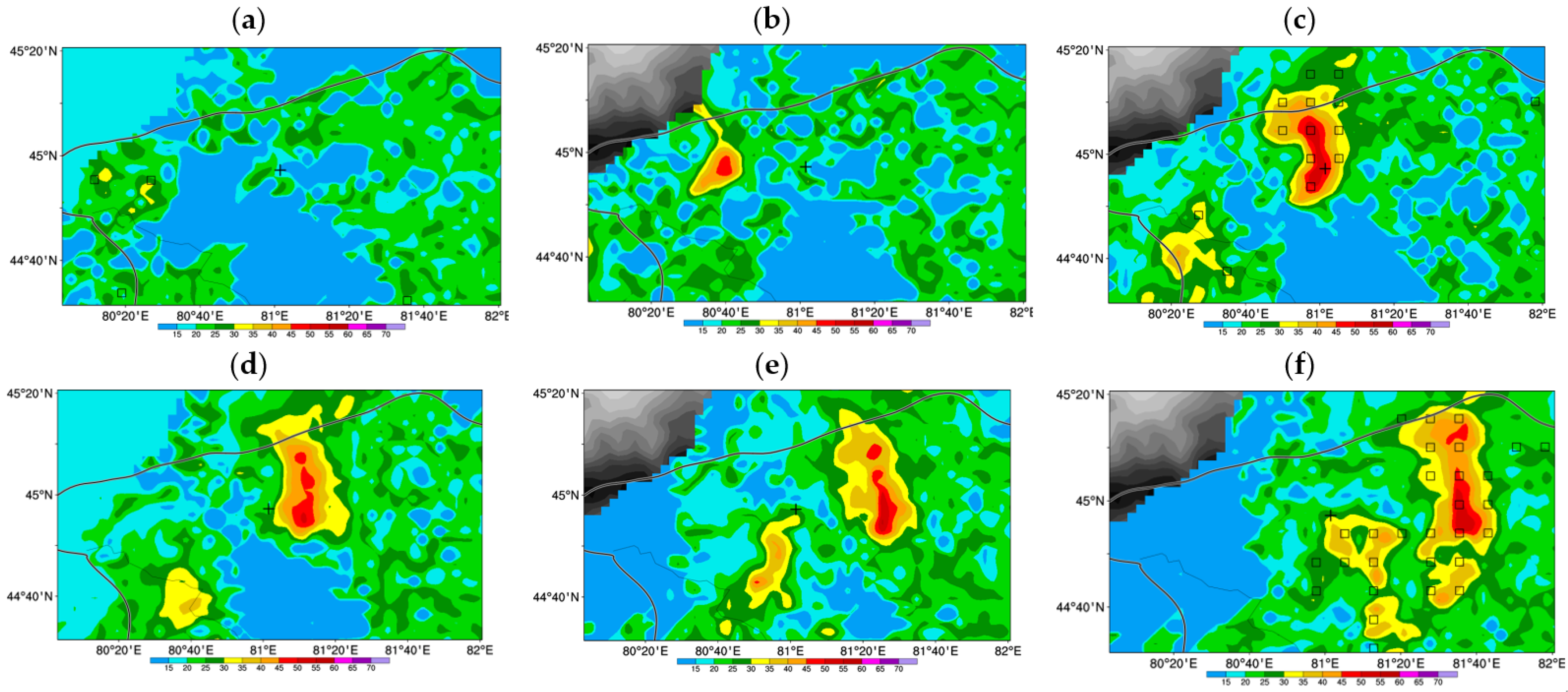
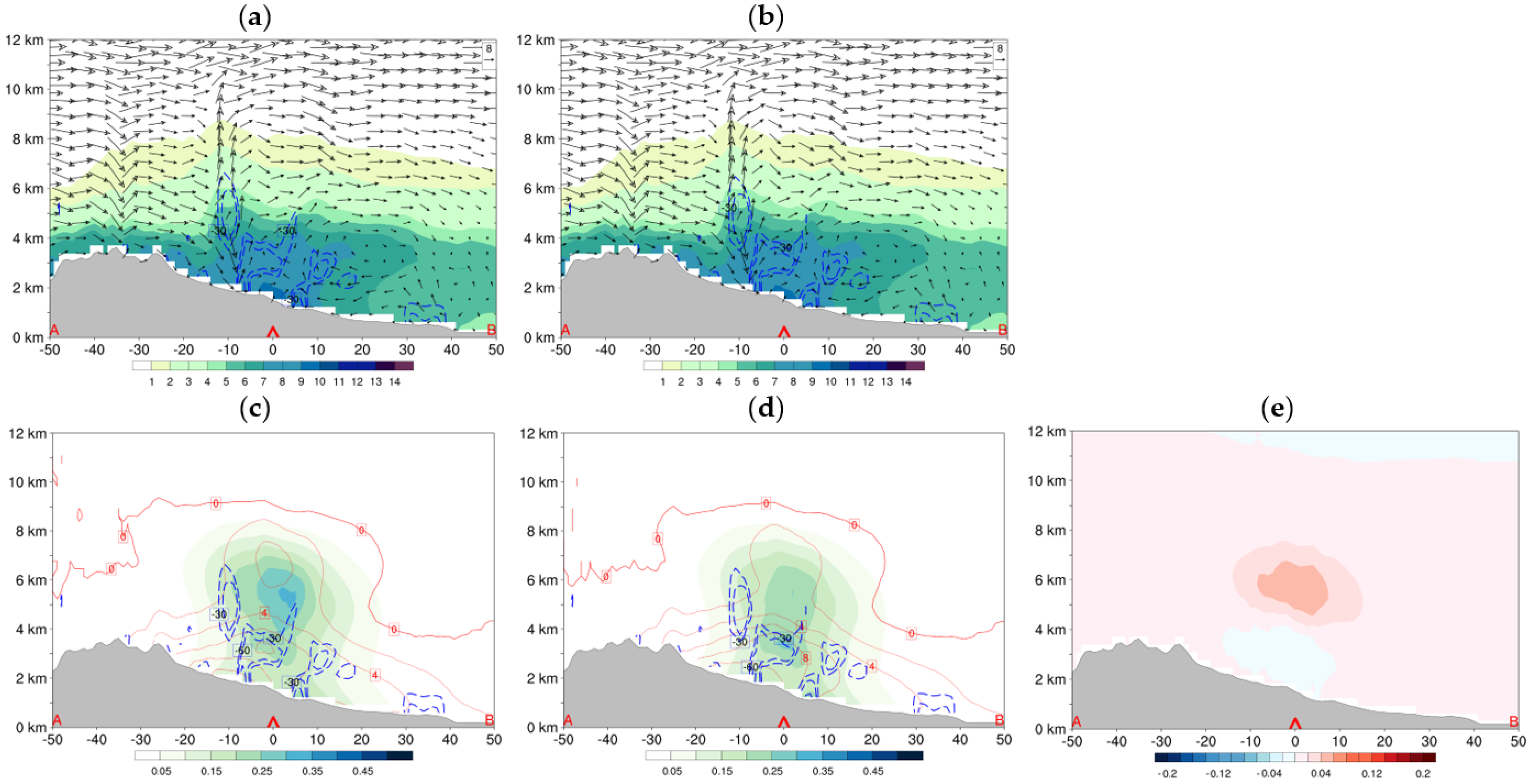
4.2. 30 July 2019 Case

On 30 July 2019, a moderate-to-heavy precipitation event lashed the central and northeastern part of Wenquan County. An hourly accumulated precipitation of more than 12.1 mm (Figure 5) in this precipitation event caused serious damage to the property and local economy in arid areas [43]. Environmental conditions (Figure 5) that are associated with sufficient water vapor condition and mid-level low pressure systems favored the development of thunderstorms across the Wenquan County. Early at 0700 UTC, the convective cells initiated in the western part of Wenquan County, then gradually moved eastward, reaching Wenquan station at about 0800 UTC. At the same time, new convective cells initiated in the southwest of Wenquan County. The two thunderstorms continued to move eastward and developed gradually, producing the moderate-to-heavy rainfall (Figure 6).
During each successive data assimilation cycle, the horizontal and vertical cross-sections of assimilated reflectivity for C2Rad (Figure 7a–c), C1Con and C3RadBy omitted show little difference between each other at 0800 UTC because very few radar observations assimilated at 0600 UTC and at 0700 UTC in which most of radar reflectivity lower than 25 dBZ. The observed and assimilated reflectivity fields have large differences at 0800 UTC in horizontal space which are displaced by about 10–30 km from each other. There are multiple thunderstorms forecasts at the western and north-eastern of Wenquan station (Figure 7a,b) which accompanied with strong ascending and descending movements (Figure 7c,d).
The analysis increment (analysis minus background) at the different vertical cross-sections of water vapor and temperature at 0800 UTC are shown in Figure 8. First of all, the water vapor has positive analysis increments near Wenquan station, as well as positive temperature increments. The positive increment of the water vapor arises because the innovation (pseudo-observations minus background) is assigned to be greater than 0% and lower than 20%. The temperature increment is a result of the water vapor observation operator minimization, and the temperature increment is pretty small [10]. Along line AB, the most significant increments of water vapor are about 0.35 g/kg in C2Rad (Figure 8c) at 5000 m, and about 0.26 g/kg in C2RadBy (Figure 8d) at 3000 m, which is accompanied with larger increments of temperature. The distribution characteristics of the analysis increments of water vapor and temperature are similar along the line of CD (Figure 9c,d). Vertical cross-sections along the lines of AB and CD near Wenquan station all exist with a negative divergence, which means it is more conducive to effective convergence of water vapor. Compared to C2Rad, C3RadBy has fewer positive analysis increments of water vapor in terms of scope and intensity between 5000 m and 7000 m.
In order to better analyze the horizontal spatial distribution of the water vapor increment, different horizontal cross-sections at 3000 m, 5000 m, 7000 m at 0800 UTC were performed (Figure 10). The positive increment of the water vapor of C2Rad (Figure 11c and Figure 12c) has more positive analysis increments than C3RadBy (Figure 11d and Figure 12d) at 5000 m (Figure 11e) and 7000 m (Figure 12e), especially at 5000 m. The most significant increments of water vapor average about 0.3 g/kg in C2Rad (Figure 11c), and 0.21 g/kg in C2RadBy (Figure 11d) at 5000 m. There is obvious wind shear between 3000 m and 5000 m at the southwestern part of Wenquan station, where the center of negative divergence in the lower ellipse exists, which is the main areal coverage of precipitation. The whole atmosphere is dominated by southwest wind at 5000 m and 7000 m, and there also exists a center of negative divergence which is favorable to precipitation in the next hour at the eastern section of Wenquan station in the upper ellipse. Showing the same data as analyzed in vertical cross-sections, C3RadBy has more positive analysis increments of water vapor at a lower atmosphere at 3000 m.
In order to further analyze the impact of water vapor assimilation to precipitation, precipitable water (PW) and convective available potential energy (CAPE) were calculated. The PW for C2Rad is greater than C2RadBy around the bottom-right side of the upper ellipse, and less than C2RadBy around the bottom side of the lower ellipse (Figure 13c). Meanwhile, the difference of CAPE between C2Rad and C2RadBy is that the value of CAPE for C2RadBy is greater than C2Rad in the lower ellipse, and almost less in the upper ellipse (Figure 13f). All of the above would impact the generation of a heavy precipitation center in Wenquan County (Figure 14).
The hourly accumulated precipitation forecast performance after water vapor assimilation was evaluated by subjective spatial distribution patterns and objective forecast skill scores at 0900 UTC 30 July 2019. The neighborhood observations of SYNOP are used for the verification. On subjective spatial distribution patterns, compared to C1Con, C2Rad and C3RadBy (Figure 14a–c) are both able to produce similar precipitation areal coverage and intensity to what was observed, but heavy precipitation at the center of Wenquan station has a position deviation. C3RadBy gives a more positive impact of the forecast, as is seen where the same intensity of a heavy precipitation center is simulated south of Wenquan station in the lower ellipse, and less impact in the southeastern part of Wenquan station in the upper ellipse (Figure 14c) than C3Rad (Figure 14b). This is proven by objective skill scores including Equitable threat score (ETS) and Bias (Figure 15). The closer ETS equals to 1, the better the forecast is; the closer Bias equals to 1, the lower the false or missing alarm rate [44]. For the ETS, E1Con achieved little forecast skill at the threshold of greater than 3.1 mm, and approached 0.22 at the thresholds of 0.1 mm which was higher than E1Rad and E1RadBy. E1Rad and E1RadBy had better ETS performance, an average increase of 20%, than E1Con at the thresholds of 3.1, and 6.1 mm, especially for E1Rad at the thresholds of 6.1 and 12.1 mm, and in E1RadBy at the thresholds of 3.1 mm. For the Bias score, the performance was different at at different thresholds. Overall, the Bias of E1Con, E1Rad, and E1RadBy at different thresholds all were lower than 1.0, which means they were missing the forecast of precipitation.

4.3. Continuous Monthly Experiments

Continuous monthly experiments from 1 July to 31 July 2019 confirmed that the updated scheme of radar reflectivity assimilation has a positive impact on the analysis of water vapor and precipitation forecast. The analysis of water vapor from E3RadBy is more close with the background than E2Rad (Figure 16a,b). The most obvious difference for distribution of the analysis increment is mainly concentrated between 3000 m and 5000 m (Figure 16c), in which the analysis increments from E2Rad are significantly greater than that from E3RadBy. The maximum probability density is about 42% (30%), and the analysis increment is 0.5 g/kg (1.2 g/kg) from E2RadBy (E2Rad).
Figure 17 shows the ETS and Bias for six hours accumulated precipitation forecast performance in Xinjiang at 1800 UTC from 1 July to 31 July 2019. For the ETS, E1Con achieved no forecast skill at the threshold of greater than 6.1 mm, and approached 0.35 and 0.27 at the thresholds of 0.1 and 3.1 mm, respectively. E1Rad and E1RadBy both have better ETS performance, an average increase of 20%, than E1Con at the thresholds of 0.1, 3.1, and 6.1 mm, especially in E1RadBy at the thresholds of 3.1 and 6.1 mm. For the Bias, the performance was similar to ETS. In addition, the Bias of E1Con, E1Rad, and E1RadBy at different thresholds all were lower than 1.0, which means they were missing the forecast of precipitation.

5. Discussion

A updated radar reflectivity assimilation scheme, instead of original scheme developed by Wang et al. [10], was implemented with the three-dimensional variational (3D-Var) system of Weather Research and Forecast (WRF). The difference between the updated and original scheme is how one retrieves the relative humidity. The original scheme assumes the relative humidity to be a fixed value where radar reflectivity is higher than a threshold. The updated scheme retrieves the relative humidity using the Bayesian method, which is consistent with clouds/precipitations provided by the model in theory. However, the possibility of disadvantages for the updated scheme exists if model is too far from the reality. For example, if a developed convective cell is observed, but there is no convection in the square window of 21 × 21 columns from the model, this will cause the lack of a supporting database for the Bayesian method [27,28]. The original scheme does not take the background hydrometeor information into account, which has less limited conditions than the updated scheme. However, the phenomenon of overpredicting precipitation may often occur when the original scheme is used in cycled data assimilation [5,10].

6. Conclusions

To verify the effect of the updated scheme on the improvement of precipitation simulation, a convective case in Wenquan County on 30 July 2019, and the continuous monthly simulation from 1 July to 31 July 2019 with contrasting experiments in Xinjiang, were performed. A single reflectivity observation test shows that relative humidity retrieval by the Bayesian method is consistent with the meteorological situation around. In the convective case, the results revealed that radar reflectivity assimilation using the original scheme and updated scheme both can increase the increment of water vapor and temperature and improve hourly precipitation forecast skill more than E1Con of the contrasting experiment. On subjective spatial distribution patterns, all the experiments can be able to produce similar areal coverage and intensity of precipitation to what is observed, but the heavy precipitation center of Wenquan County has a position deviation. The C3RadBy using the updated scheme gives more positive impact to the forecast. On objective skill scores, the E1Rad and E1RadBy have better ETS performance than E1Con at the thresholds of 3.1, and 6.1 mm, especially in E1Rad at the thresholds of 6.1 and 12.1 mm, and in E1RadBy at the threshold of 3.1 mm.
The continuous monthly experiments further proved that ingesting Doppler radar information could help improve the analysis and short-term (6 h) precipitation forecast skill in Xinjiang more than the contrasting experiments. The analysis of water vapor is closer with the background in the updated scheme than the original scheme. The most obvious difference for distribution of the analysis increment is mainly concentrated between 3000 m and 5000 m. E1Rad and E1RadBy both have better ETS performance than E1Con at the thresholds of 0.1, 3.1, and 6.1 mm, especially in E1RadBy at the thresholds of 3.1 and 6.1 mm.
In this study, the Bias of all the experiments at different thresholds all were lower than 1.0, which means they were missing the forecast of precipitation. To make better use of radar reflectivity data, future work should consider assimilating all the radar reflectivity whether or not greater than 25 dBZ, and combine advantages from the updated scheme and the original scheme.

Author Contributions

Conceptualization, M.A. and S.F.; methodology, J.L.; software, J.L. and H.L.; validation, H.Z. and H.L.; formal analysis, H.L.; investigation, M.A.; writing, original draft preparation, J.L.; writing, review, and editing, J.L., Y.W. and A.A. All authors have read and agreed to the published version of the manuscript.

Funding

This work was supported by Xinjiang Meteorological Bureau Research Fund (Grant No. YD202205, MS201908, 2021-45), Flexible Talents Introducing Project of Xinjiang (Grant No.2021-49), National Key Research and Development Program (Grant No. 2018YFC1507105).

Data Availability Statement

All the data used in this work can be available upon request to the corresponding author.

Conflicts of Interest

The authors declare no conflict of interest.

References

  1. Sun, J.; Crook, N.A. Dynamical and microphysical retrieval from Doppler radar observations using a cloud model and its adjoint. Part I: Model development and simulated data experiments. J. Atmos. Sci. 1997, 54, 1642–1661. [Google Scholar] [CrossRef]
  2. Gao, J.; Xue, M.; Shapiro, A.; Droegemeier, K.K. A variational analysis for the retrieval of three-dimensional mesoscale wind fields from two Doppler radars. Mon. Weather Rev. 1999, 127, 2128–2142. [Google Scholar] [CrossRef]
  3. Gao, J.; Xue, M.; Brewster, K.; Droegemeier, K.K. A three-dimensional data analysis method with recursive filter for Doppler radars. J. Atmos. Ocean. Technol. 2004, 21, 457–469. [Google Scholar] [CrossRef]
  4. Sun, J. Convective-scale assimilation of radar data: Progress and challenges. Q. J. R. Meteorol. Soc. J. Atmos.Sci. Appl. Meteorol. Phys. Oceanogr. 2005, 131, 3439–3463. [Google Scholar] [CrossRef]
  5. Hu, M.; Xue, M.; Brewster, K. 3DVAR and cloud analysis with WSR-88D Level-II data for the prediction of the Fort Worth tornadic thunderstorms. Part I: Cloud analysis and its impact. Mon. Weather Rev. 2006, 134, 675–698. [Google Scholar] [CrossRef]
  6. Tong, C.C. Limitations and Potential of Complex Cloud Analysis and Its Improvement for Radar Reflectivity Data Assimilation Using OSSES. Ph.D. Thesis, University of Oklahoma, Norman, OK, USA, 2015. [Google Scholar]
  7. Xue, M.; Wang, D.; Gao, J.; Brewster, K.A.; Droegemeier, K.K. The Advanced Regional Prediction System (ARPS), storm-scale numerical weather prediction and data assimilation. Meteorol. Atmos. Phys. 2003, 82, 139–170. [Google Scholar] [CrossRef]
  8. Gao, J.; Stensrud, D.J. Assimilation of reflectivity data in a convective-scale, cycled 3DVAR framework with hydrometeor classification. J. Atmos. Sci. 2012, 69, 1054–1065. [Google Scholar] [CrossRef]
  9. Gao, J.; Smith, T.M.; Stensrud, D.J.; Fu, C.; Calhoun, K.; Manross, K.L.; Brogden, J.; Lakshmanan, V.; Wang, Y.; Thomas, K.W.; et al. A real-time weather-adaptive 3DVAR analysis system for severe weather detections and warnings. Weather Forecast. 2013, 28, 727–745. [Google Scholar] [CrossRef]
  10. Wang, H.; Sun, J.; Fan, S.; Huang, X.Y. Indirect assimilation of radar reflectivity with WRF 3D-Var and its impact on prediction of four summertime convective eventsss. J. Appl. Meteorol. Climatol. 2013, 52, 889–902. [Google Scholar] [CrossRef]
  11. Wang, H.; Sun, J.; Zhang, X.; Huang, X.Y.; Auligne, T. Radar data assimilation with WRF 4D-Var. Part I: System development and preliminary testing. Mon. Weather Rev. 2013, 141, 2224–2244. [Google Scholar] [CrossRef]
  12. Xiao, Q.; Sun, J. Multiple-radar data assimilation and short-range quantitative precipitation forecasting of a squall line observed during IHOP_2002. Mon. Weather Rev. 2007, 135, 3381–3404. [Google Scholar] [CrossRef]
  13. Aksoy, A.; Dowell, D.C.; Snyder, C. A multicase comparative assessment of the ensemble Kalman filter for assimilation of radar observations. Part I: Storm-scale analyses. Mon. Weather Rev. 2009, 137, 1805–1824. [Google Scholar] [CrossRef] [Green Version]
  14. Dowell, D.C.; Wicker, L.J.; Snyder, C. Ensemble Kalman filter assimilation of radar obervations of the 8 May 2003 Oklahoma City supercell: Influences of reflectivity observations on storm-scale analyses. Mon. Weather Rev. 2011, 139, 272–294. [Google Scholar] [CrossRef] [Green Version]
  15. Gao, J.; Fu, C.; Stensrud, D.J.; Kain, J.S. OSSEs for an ensemble 3DVAR data assimilation system with radar observations of convective storms. J. Atmos. Sci. 2016, 73, 2403–2426. [Google Scholar] [CrossRef]
  16. Lai, A.; Gao, J.; Koch, S.E.; Wang, Y.; Pan, S.; Fierro, A.O.; Cui, C.; Min, J. Assimilation of Radar Radial Velocity, Reflectivity, and Pseudo–Water Vapor for Convective-Scale NWP in a Variational Framework. Mon. Weather Rev. 2019, 147, 2877–2900. [Google Scholar] [CrossRef]
  17. Albers, S.C.; McGinley, J.A.; Birkenheuer, D.L.; Smart, J.R. The Local Analysis and Prediction System (LAPS): Analyses of clouds, precipitation, and temperature. Weather Forecast. 1996, 11, 273–287. [Google Scholar] [CrossRef]
  18. Sun, J.; Wang, H.L. Radar data assimilation with WRF 4D-Var. Part II: Comparison with 3D-Var for a squall line over the U.S. Great Plains. Mon. Weather Rev. 2013, 141, 2245–2264. [Google Scholar] [CrossRef]
  19. Schenkman, A.D.; Ming, X.; Shapiro, A.; Brewster, K.; Gao, J. The analysis and prediction of the 8–9 May 2007 Oklahoma tornadic mesoscale convective system by assimilation WSR-88D and CASA radar data using 3DVAR. Mon. Weather Rev. 2011, 139, 224–246. [Google Scholar] [CrossRef] [Green Version]
  20. Tong, M.J.; Xue, M. Ensemble Kalman filter assimilation of Doppler radar data with a compressible nonhydrostatic model: OSS experiments. Mon. Weather Rev. 2005, 133, 1789–1807. [Google Scholar] [CrossRef] [Green Version]
  21. Xu, Q. Generalized adjoint for physical processes with parameterized discontinuities. Part I: Basic issues and heuristic examples. J. Atmos. Sci. 1996, 53, 1123–1142. [Google Scholar] [CrossRef]
  22. Ge, G.; Gao, J.; Xue, M. Impacts of assimilating measurements of different state variables with a simulated supercell storm and three-dimensional variational method. Mon. Weather Rev. 2013, 141, 2759–2777. [Google Scholar] [CrossRef] [Green Version]
  23. Walbröl, A.; Crewell, S.; Engelmann, R.; Orlandi, E.; Griesche, H.; Radenz, M.; Hofer, J.; Althausen, D.; Maturilli, M.; Ebell, K. Atmospheric temperature, water vapor and liquid water path from two microwave radiometers during MOSAiC. Sci. Data 2022, 9, 534. [Google Scholar] [CrossRef] [PubMed]
  24. Shikhovtsev, A.Y.; Khaikin, V.B.; Mironov, A.P.; Kovadlo, P.G. Statistical Analysis of the Water Vapor Content in North Caucasus and Crimea. Atmos. Ocean Opt. 2022, 35, 168–175. [Google Scholar] [CrossRef]
  25. Philipona, R.; Kräuchi, A.; Kivi, R.; Peter, T.; Wild, M.; Dirksen, R.; Fujiwara, M.; Sekiguchi, M.; Hurst, D.F.; Becker, R. Balloon-borne radiation measurements demonstrate radiative forcing by water vapor and clouds. Meteorol. Z. 2020, 29, 501–509. [Google Scholar] [CrossRef]
  26. Wang, H.; Hu, Z.; Liu, P.; Zhang, F. Impact of Water Vapor on the Development of a Supercell Over Eastern China. Front. Earth Sci. 2022, 10, 881579. [Google Scholar] [CrossRef]
  27. Caumont, O.; Ducrocq, V.; Wattrelot, E.; Jaubert, G.; Pradier-Vabre, S. 1D+3DVar assimilation of radar reflectivity data: A proof of concept. Tellus 2010, 62A, 173–187. [Google Scholar] [CrossRef]
  28. Wattrelot, E.; Caumont, O.; Mahfouf, J.F. Operational implementation of the 1D+3D-Var assimilation method of radar reflectivity data in the AROME model. Mon. Weather Rev. 2014, 142, 1852–1873. [Google Scholar] [CrossRef] [Green Version]
  29. Kummerow, C.; Hong, Y.; Olson, W.S.; Yang, S.; Adler, R.F.; McCollum, J.; Ferraro, R.; Petty, G.; Shin, D.B.; Wilheit, T.T. The evolution of the Goddard profiling algorithm (GPROF) for rainfall estimation from passive microwave sensors. J. Appl. Meteor. 2001, 40, 1801–1820. [Google Scholar] [CrossRef]
  30. Olson, W.S.; Kummerow, C.D.; Heymsfield, G.M.; Giglio, L. A method for combined passive-active microwave retrievals of cloud and precipitation profiles. J. Appl. Meteor. 1996, 35, 1763–1789. [Google Scholar] [CrossRef]
  31. Lorenc, A.C. Analysis methods for numerical weather prediction. Q. J. R. Meteor. Soc. 1986, 112, 1177–1194. [Google Scholar] [CrossRef]
  32. Barker, D.M.; Huang, W.; Guo, Y.R.; Bourgeois, A. A three-dimensional variational (3DVAR) data assimilation system for use with MM5. NCAR Tech. Note 2003, 68. [Google Scholar]
  33. Parrish, D.F.; Derber, J.C. The National Meteorological Center’s spectral statistical-interpolation analysis system. Mon. Weather Rev. 1992, 120, 1747–1763. [Google Scholar] [CrossRef]
  34. Bannister, R.N. A review of forecast error covariance statistics in atmospheric variational data assimilation. II: Modelling the forecast error covariance statistics. Q. J. R.Meteor. Soc. 2008, 134, 1971–1996. [Google Scholar] [CrossRef]
  35. Skamarock, W.C.; Klemp, J.B.; Dudhia, J.; Gill, D.O.; Barker, D.; Duda, M.G.; Powers, J.G. A Description of the Advanced Research WRF Version 3 (No. NCAR/TN-475+STR). University Corporation for Atmospheric Research. 2008. Available online: https://opensky.ucar.edu/islandora/object/technotes:500 (accessed on 15 August 2021).
  36. National Center for Atmospheric Research. The Research Data Archive. Available online: https://rda.ucar.edu/datasets/ (accessed on 10 August 2021).
  37. Hong, S.-Y.; Lim, J.-O.J. The WRF single-moment 6-class microphysics scheme (WSM6). J. Korean Meteor. Soc. 2006, 42, 129–151. [Google Scholar]
  38. Iacono, M.J.; Delamere, J.S.; Mlawer, E.J.; Shephard, M.W.; Clough, S.A.; Collins, W.D. Radiative forcing by long–lived greenhouse gases: Calculations with the AER radiative transfer models. J. Geophys. Res. 2008, 113, D13103. [Google Scholar] [CrossRef]
  39. Tewari, M.; Chen, F.; Wang, W.; Dudhia, J.; LeMone, M.A.; Mitchell, K.; Ek, M.; Gayno, G.; Wegiel, J.; Cuenca, R.H. Implementation and verification of the unified NOAH land surface model in the WRF model. In Proceedings of the 20th Conference on Weather Analysis and Forecasting/16th Conference on Numerical Weather Prediction, Seattle, WA, USA, 12–16 January 2004; pp. 11–15. [Google Scholar]
  40. Kain, J.S. The Kain–Fritsch convective parameterization: An update. J. Appl. Meteor. 2004, 43, 170–181. [Google Scholar] [CrossRef]
  41. Pleim, J.E. A Combined Local and Nonlocal Closure Model for the Atmospheric Boundary Layer. Part I: Model Description and Testing. J. Appl. Meteor. Climatol. 2007, 46, 1383–1395. [Google Scholar] [CrossRef]
  42. National Meteorological Information Center. China Meteorological Data Sharing Service System. Available online: http://data.cma.cn/ (accessed on 23 August 2021).
  43. Peng, L.; Yang, Y.; Xin, Y.; Wang, C. Impact of Lightning Data Assimilation on Forecasts of a Leeward Slope Precipitation Event in the Western Margin of the Junggar Basin. Remote Sens. 2021, 13, 3584. [Google Scholar] [CrossRef]
  44. Clark, A.J.; Xue, M.; Weisman, M.L. Neighborhood based verification of precipitation forecasts from convection allowing NCAR WRF Model simulations and the operational NAM. Weather Forecast. 2010, 25, 1495–1509. [Google Scholar] [CrossRef]
Figure 1. Flowchart of the sequence of operations of water vapor retrieval and assimilation.
Remotesensing 14 05897 g001
Figure 2. (a) The model forecast domains and observations assimilated. The outside box indicates domain 1, and the inner black box indicates domain 2. The red dots indicate SYNOP stations. (b) The radar station and radar data assimilated available range in domain 2. The location of Wenquan national meteorological station, west of Bole’s radar, is represented by the back cross marker which is same below. The black dots show the locations of the nine radar stations. The altitude (unit m) of ground above sea level is represented by the colour shades.
Remotesensing 14 05897 g002
Figure 3. Flowcharts of spin-up, data assimilation, and forecast for the (a) convective case and (b) continuous monthly experiments.
Remotesensing 14 05897 g003
Figure 4. The single reflectivity (unit dBZ) observation test of the relative humidity (unit %) retrieved at 12th model level. (a) Assimilated reflectivity. (b) Observed reflectivity. (c) Weight of each assimilated reflectivity. (d) Assimilated relative humidity. (e) Relative humidity retrieved using the updated scheme. (f) Relative humidity retrieved using the original scheme. The black square indicates the window of 21 × 21 grid points used for the Bayesian method. The red square indicates the single reflectivity observation point.
Remotesensing 14 05897 g004
Figure 5. Environmental conditions with the geopotential height (unit gpm, blue lines), wind vector (unit m/s, wind bars), temperature (unit °C, red lines) at 500 hPa, and relative humidity (unit %, colour shades) at 750 hPa at (a) 0000 UTC, (b) 0600 UTC 30 July 2019 from NCEP-FNL.
Remotesensing 14 05897 g005
Figure 6. Observed composite reflectivity fields (unit dBZ) at (a) 0700 UTC, (b) 0730 UTC, (c) 0800 UTC, (d) 0820 UTC, (e) 0840 UTC, and (f) 0900 UTC 30 July 2019. The black squares indicate the reflectivity assimilated, in which observed radar reflectivity is higher than 25 dBZ which is same below. The shades of gray indicate the model terrain height in each plot which is same below.
Remotesensing 14 05897 g006
Figure 7. Horizontal and vertical cross-sections of assimilated composite reflectivity fields (unit dBZ) from (a) C2Rad for 1-h forecasts beginning at 0700 UTC 30 July 2019. The wind vector (unit m/s, black arrows) is calculated by u and w wind in which w speed is multiplied by 10.0 in (b,c) which is the same below. The red triangle in each plot of vertical cross-sections indicates the location of Wenquan station. The red lines indicate vertical cross-sections through AB and CD. The color points indicate the vertical distribution of observed reflectivity fields (unit dBZ).
Remotesensing 14 05897 g007
Figure 8. Vertical cross-section of the analysis and the increment of water vapor (unit g/kg) along line AB at 0800 UTC. (a) The analysis from C2Rad. (b) The analysis from C2RadBy. (c) The increment from C2Rad. (d) The increment from C2RadBy. (e) The difference of increment between C2Rad and C2RadBy. The shades in each plot indicate the water vapor mixing ratio (unit g/kg). The solid red lines indicate the increment of temperature (unit 0.001 °C). The dashed blue lines indicate negative divergence (unit 1/s).
Remotesensing 14 05897 g008
Figure 9. Vertical cross-section of the analysis and the increment of water vapor (unit g/kg) along line CD at 0800 UTC. (a) The analysis from C2Rad. (b) The analysis from C2RadBy. (c) The increment from C2Rad. (d) The increment from C2RadBy. (e) The difference of increment between C2Rad and C2RadBy. The shades in each plot indicate the water vapor mixing ratio (unit g/kg). The solid red lines indicate the increment of temperature (unit 0.001 °C). The dashed blue lines indicate negative divergence (unit 1/s).
Remotesensing 14 05897 g009
Figure 10. Horizontal cross-section of the analysis and the increment of water vapor (unit g/kg) at 0800 UTC at 3000m. (a) The analysis from C2Rad. (b) The analysis from C2RadBy. (c) The increment from C2Rad. (d) The increment from C2RadBy. (e) The difference of increment between C2Rad and C2RadBy. The shades in each plot indicate the water vapor mixing ratio (unit g/kg). The solid red lines indicate the increment of temperature (unit 0.001 °C). The dashed blue lines indicate the analysis of negative divergence (unit 1/s). The ellipse of dashed red lines indicates the main areal coverage of precipitation which is the same below.
Remotesensing 14 05897 g010
Figure 11. Horizontal cross-section of the analysis and the increment of water vapor (unit g/kg) at 0800 UTC at 5000 m. (a) The analysis from C2Rad. (b) The analysis from C2RadBy. (c) The increment from C2Rad. (d) The increment from C2RadBy. (e) The difference of increment between C2Rad and C2RadBy. The shades in each plot indicate the water vapor mixing ratio (unit g/kg). The solid red lines indicate the increment of temperature (unit 0.001 °C). The dashed blue lines indicate the analysis of negative divergence (unit 1/s).
Remotesensing 14 05897 g011
Figure 12. Horizontal cross-section of the analysis and the increment of water vapor (unit g/kg) at 0800 UTC at7000 m. (a) The analysis from C2Rad. (b) The analysis from C2RadBy. (c) The increment from C2Rad. (d) The increment from C2RadBy. (e) The difference of increment between C2Rad and C2RadBy. The shades in each plot indicate the water vapor mixing ratio (unit g/kg). The solid red lines indicate the increment of temperature (unit 0.001 °C). The dashed blue lines indicate the analysis of negative divergence (unit 1/s).
Remotesensing 14 05897 g012
Figure 13. The increment and difference of precipitable water (PW, unit mm) and convective available potential energy (CAPE, unit J/kg) at 0800 UTC 30 July 2019. (a) The increment of PW from C2Rad. (b) The increment of PW from C2RadBy. (c) The difference of PW between (a,b). (d) The increment of CAPE from C2RadBy. (e) The increment of CAPE from C2RadBy. (f) The difference of CAPE between (d,e).
Remotesensing 14 05897 g013
Figure 14. Hourly accumulated precipitation of (a) C1Con, (b) C1Rad, and (c) C3RadBy at 0900 UTC. The colored dots show the locations and hourly accumulated precipitation (in millimeters) of observations of SYNOP. The Forecast hourly accumulated precipitation (unit mm) is represented by the colour shades.
Remotesensing 14 05897 g014
Figure 15. Taylor diagrams of the hourly accumulated precipitation forecast at 0900 UTC from 30 July 2019. The triangle and circle indicate the increased percentage of ETS relative to C1Con or E1Con which is the same below.
Remotesensing 14 05897 g015
Figure 16. Diagnostic plots of water vapor (unit g/kg). (a) Scatter distribution of water vapor mixing ratio between analysis and background. (b) QQ distribution of water vapor mixing ratio. (c) The distribution of the analysis increment at different altitudes (unit m) of ground above sea level. (d) PDF distribution of the analysis increment. The blue lines and circles indicate E3RadBy, and the red lines and circles indicate E2Rad.
Remotesensing 14 05897 g016
Figure 17. Taylor diagrams of the six hours accumulated precipitation forecast at 1800 UTC from 1 July to 31 July 2019.
Remotesensing 14 05897 g017
Table 1. Experimental configurations of the WRF model.
Model and Configurations
Versionv3.9.1, nonhydrostatic = true
Domain 1712 × 532, nominal 9 km
Domain 2832 × 652, nominal 3 km
Vertical computation layers50
Pressure top10 hPa
Lateral boundary conditionsNCEP-FNL
MicrophysicsWSM6
Longwave radiationRRTMG
Shortwave radiationRRTMG
Land surfaceUnified Noah land-surface model
Deep convectionKain–Fritsch
Planetary-boundary and surface layerACM2
Table 2. List of Experiments.
ExperimentsObservationsPseudo Water Vapor
30 July 2019 caseC1ConDomain 1: SYNOP
Domain 2: SYNOP + radar radial velocity
_
C2RadDomain 1: SYNOP
Domain 2: SYNOP + radar radial velocity + reflectivity
The original scheme:
Y p o q v = Y p o r h × X q s , With
Y p o r h = 85 % ,   25 Y Z 40 ,
Y p o r h = 95 % ,   40 < Y Z 50 .
C3RadBySame as C2RadThe updated scheme:
Y p o q v = Y p o r h × X q s , With
Y p o r h = i X i r h ω i j ω j .
July 2019 Continuous experimentsE1ConSame as C1Con_
E2RadSame as C2RadSame as C2Rad
E3RadBySame as C2RadSame as C3RadBy
Publisher’s Note: MDPI stays neutral with regard to jurisdictional claims in published maps and institutional affiliations.

