1. Introduction
Semantic segmentation tasks classify each pixel in an image into several regions with specific semantic categories and often appear in fields such as human–computer interaction, computer photography, image search engines, and augmented reality. In these applications, the extraction targets are usually clear in semantics and have a small coverage area. However, things are different in remote sensing images. The targets in remote sensing images have a wider range of distribution and more complex features. On the one hand, such characteristics provide richer target detail information for feature detection, such as color, contour, and texture. On the other hand, much more complex interference is introduced into segmentation tasks.
The traditional remote sensing image segmentation methods mainly include support vector machine (SVM) methods [
1], superpixel-based methods [
2], and semisupervised geodesic-based methods [
3]. Traditional methods can achieve better results with a small sample size. Still, with the increase in sample data, the accuracy of traditional methods has not significantly improved to meet the application requirements. Usually, traditional methods are only effective for some specific scenarios, with poor universality.
Focused on the above situation, compared with traditional methods in machine learning, Deep Convolutional Neural Networks (DCNNs), such as FCN [
4], have shown excellent feature extraction and object representation abilities [
5]. Many approaches have been proposed to increase the receptive field of convolutional neural networks. Unet [
6] and SegNet [
7] propose skip connection, trying to connect the same-sized feature maps in the encoder and decoder layers. The DeepLab series network models are all based on encoder–decoder architecture. Atrous convolution to expand the receptive field is introduced in DeepLab v1 [
8] and DeepLab v2 [
9]. Furthermore, Atrous Spatial Pyramid Pooling (ASPP) was proposed to expand the perceptual field further and enhance the spatial feature extraction capability using multi-layer cavity convolution. DeepLab v3 [
10] introduced image-level multiscale features in ASPP to further improve the feature extraction capability. DeepLab v3+ [
11] used a modified Xception [
12] encoder and a lightweight decoder to improve the resolution of segmentation results. FarSeg [
13] uses two encoder branches to enhance the extraction of foreground and background, respectively. In addition, some studies have been conducted to improve the deep learning methods according to the characteristics of remote sensing images. EFCNet [
14] introduces the separable convolutional module (SCM) to alleviate the problem of numerous parameters for the semantic segmentation of high-resolution remote sensing images. DSPCANet [
15] introduces the internal residual block (R2_Block) to enhance the receptive field of the network and learn the ground feature representation from additional DSM images. Sharifi et al. [
16] proposed the ResUNet-a model with post-processing. The model contains the output of joint connection, which significantly improves the efficiency and robustness of the farmland extraction model. However, stacking and aggregating convolutional layers perform poorly in covering global receptive fields. Additionally, these methods do not effectively extract global contextual information.
A helpful method for obtaining global contextual information is the self-attention mechanism. Nonlocal [
17] proposes a generalized, simple, nonlocal operation operator that can be directly embedded into neural networks. DANet [
18] introduces the self-attention mechanism to capture feature dependencies in the spatial and channel dimensions. A2-Nets [
19], expectation–maximization attention networks [
20], and CBAM [
21] introduced a self-attention mechanism to merge global features by different descriptors. LANet [
22] proposes a patch attention module and an attention embedding module to merge high-level and low-level features in the model. HMANet [
23] proposes a class augmented attention module to obtain class-level information. SSFTT [
24] utilizes the self-attention mechanism to construct 3D and 2D convolutional layers to jointly extract shallow spectral and spatial features. However, methods that rely on self-attention only cause the network to pay attention to itself and overlook the spatial context relationship hidden in the labels.
To solve the above-mentioned issues, we suggest a brand new structure termed the Label Attention Module (LAM). LAM fully uses the label’s spatial context via the attention module. However, the way to generate attention is different than the self-attention module. LAM optimizes the attention probability map by introducing label information.
Furthermore, we proposed a triple-attention network called TANet, which contains LAM and two self-attention modules presented in DANet: PAM and CAM. TANet can help enhance semantic segmentation accuracy due to the triple attention module’s ability to strengthen global information extraction.
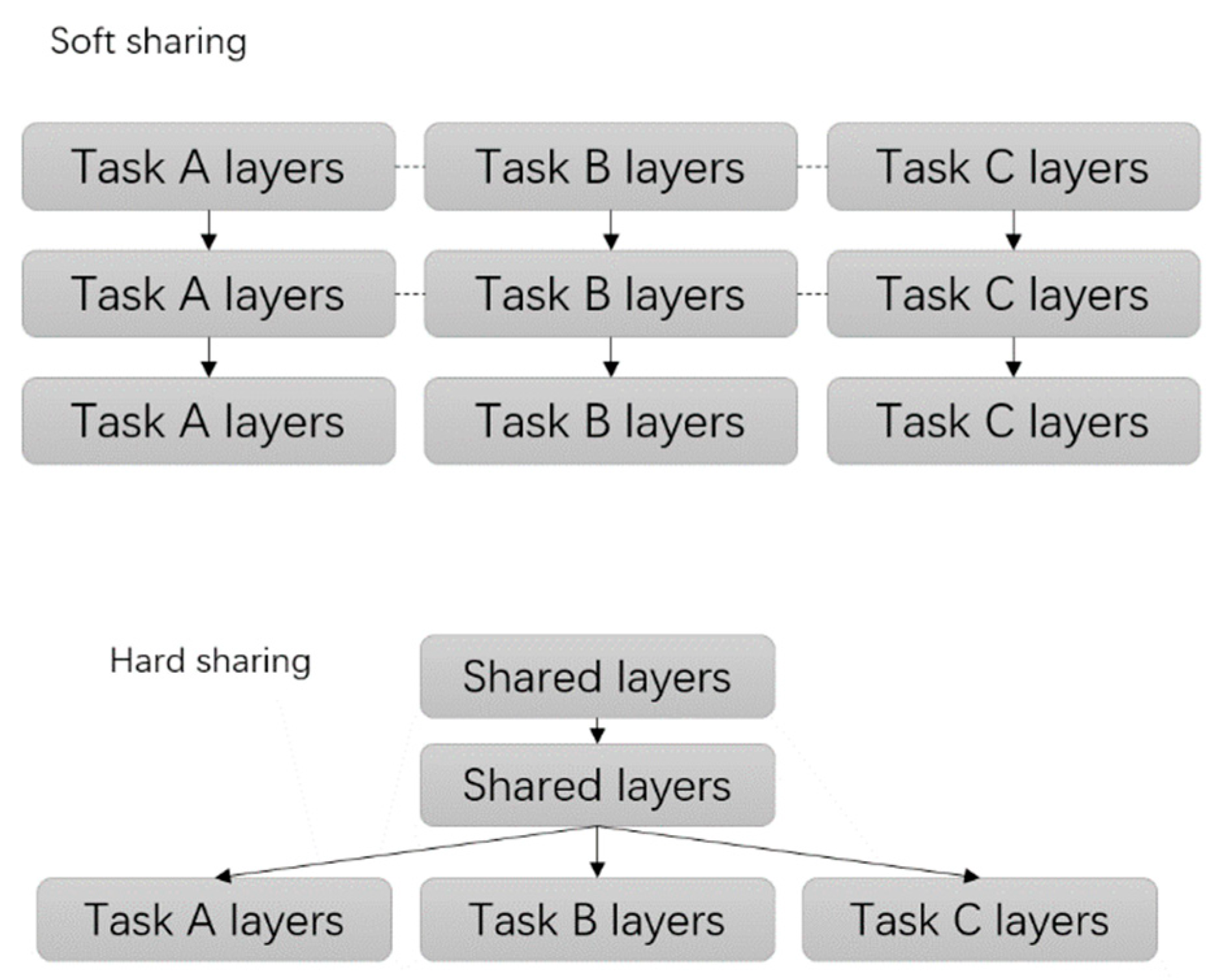
Adding LAM can significantly increase the segmentation accuracy of a large range of targets. However, misjudgment problems would appear with respect to some targets presenting similar features, such as impervious surfaces and concrete roof buildings. Due to the competition between different categories, the probability of the misjudgment category affects the real category. In order to reduce the competition between categories, we introduced a multi-task mechanism. The multi-task mechanism converts a multi-category segmentation task into multiple binary-classification segmentation tasks. All categories share an encoder, and each category owns a separate decoder. The multi-task architecture can effectively improve the segmentation accuracy of similar categories. Furthermore, we perform some edge optimization to improve the accuracy of the edge area of different categories. The edge optimization includes two new edge branches and an edge attention module. Combined with the triple attention and multi-task architecture mentioned above, the model contains four attention modules, so we name this network Multi-Task Quadruple Attention Network. We conducted experiments on two public datasets (Potsdam and Vaihingen datasets) and a self-made dataset (CZ-WZ dataset) to demonstrate the effectiveness of the proposed model.
The main contributions of this paper are as follows:
- (1)
We propose the label attention module (LAM) to learn the spatial contextual information of features from the label instead of information from the network itself.
- (2)
A Triple Attention Network is designed to obtain global features of large objects. It significantly improves the semantic segmentation accuracy of large objects in remote sensing images.
- (3)
A Multi-task TANet (MTANet) architecture is proposed to reduce the misjudgment between similar categories.
- (4)
Based on the MTANet model, A MQANet model is constructed to optimize the edge area of semantic segmentation.
3. Methodology
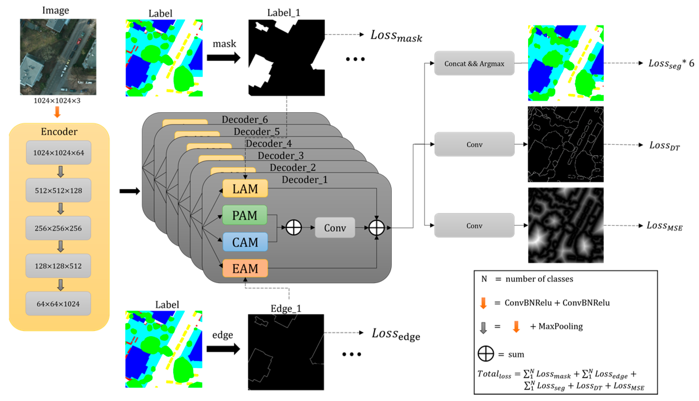
The proposed network model consists of encoder, decoder, and edge optimization module. The encoder structure is the same as the VGG architecture adopted by UNet. For the decoder, the proposed network converts a multi-category semantic segmentation task into multiple binary-segmentation tasks. The number of decoders is the same as the number of semantic segmentation categories of the ground object. Each decoder contains quadruple attention modules, PAM, CAM, LAM, and EAM. The optimization algorithm for edge extraction consists of three parts, the edge map branch, the distance map branch, and the edge attention module. The architecture of the proposed method is shown in
Figure 2.
Section 3.1 and
Section 3.2 describe the PAM, CAM, and LAM. In
Section 3.3, we introduce the multi-task architecture of this network. In
Section 3.4, edge optimization is introduced, including two edge map branches and the EAM.
In
Figure 2, all categories share one encoder, and each category owns a separate triple attention decoder. Each decoder contains four attention modules. LAM needs label information, and EAM needs edge labels during training.
3.1. PAM and CAM
Similar to human learning, machine learning is considered attention. The attention mechanism’s core goal is to find critical information from various information items for the current task. Position Attention Module (PAM) and Channel Attention Module (CAM) are practical self-attention modules. PAM captures spatial global dependencies, and CAM pays attention to the importance of each channel dimension.
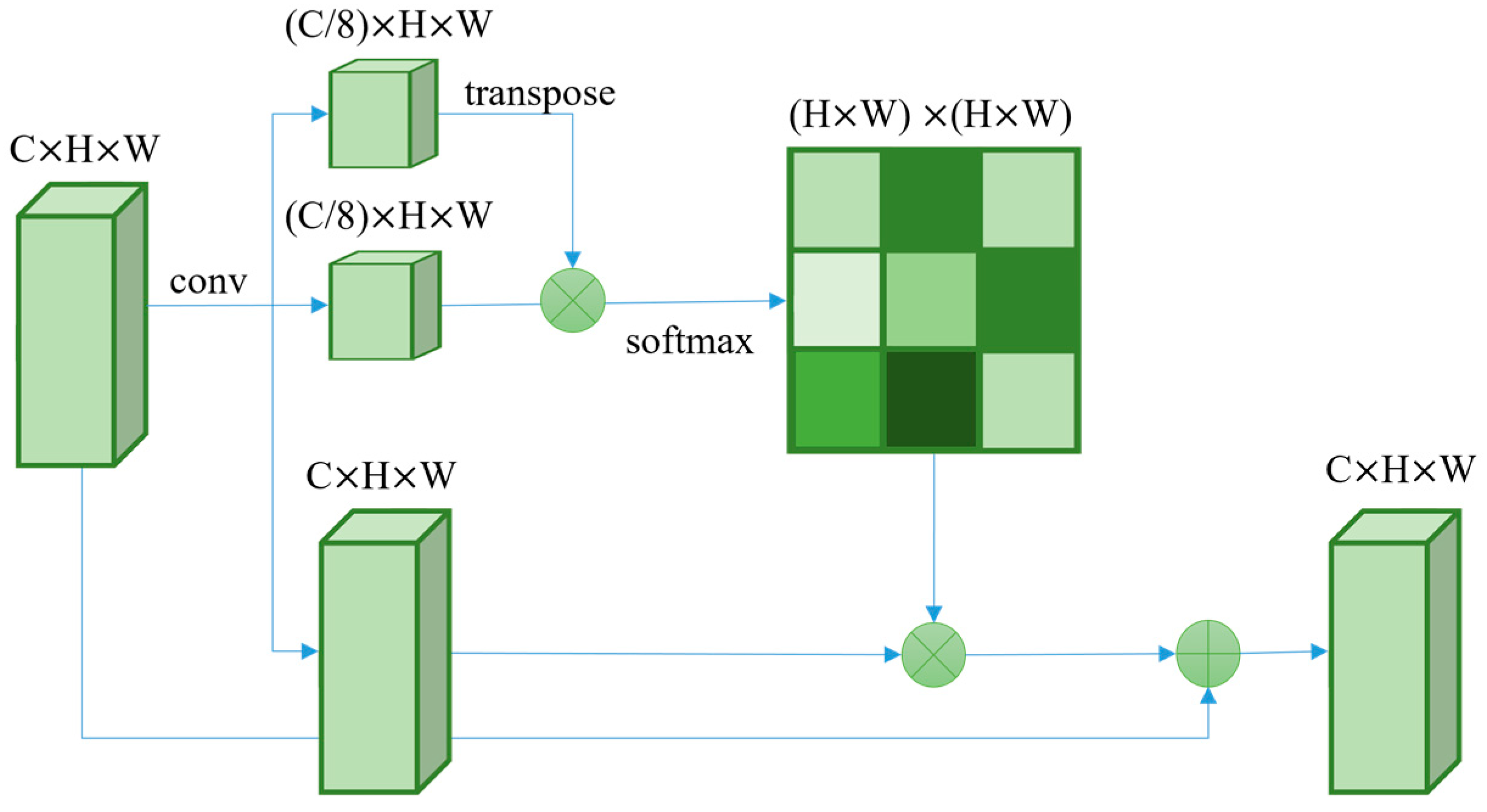
Figure 3 illustrates the structure of the PAM. In the PAM, the input generates two parts of feature maps: one is represented as
and
to calculate an attention probability map in the shape (
×
) × (
×
), and the other is used as
.
,
, and
denote query features, key features, and value features. Furthermore,
,
, and
represent the attention probability map’s channel, height, and weight. Then, the optimization attention map is reshaped to obtain the final prediction map.
The overall structure of the PAM is shown in Equation (2).
where
denotes the attention probability map calculated, and
is the final output, obtained by summing the input and the optimization attention map.
refers to the size of the feature map reshape to
.
The width and height of the feature are multiplied by a large value and reduce the number of channels to one-eighth of the original one by using convolution to facilitate operations. Then the dimension of the number of channels is eliminated by matrix multiplication. This operation does not affect the shape of the feature.
PAM uses a spatial attention map to select aggregating contexts. In addition, PAM has a global contextual view. Similar semantic features enhance intra-class compactness and semantic consistency [
18].
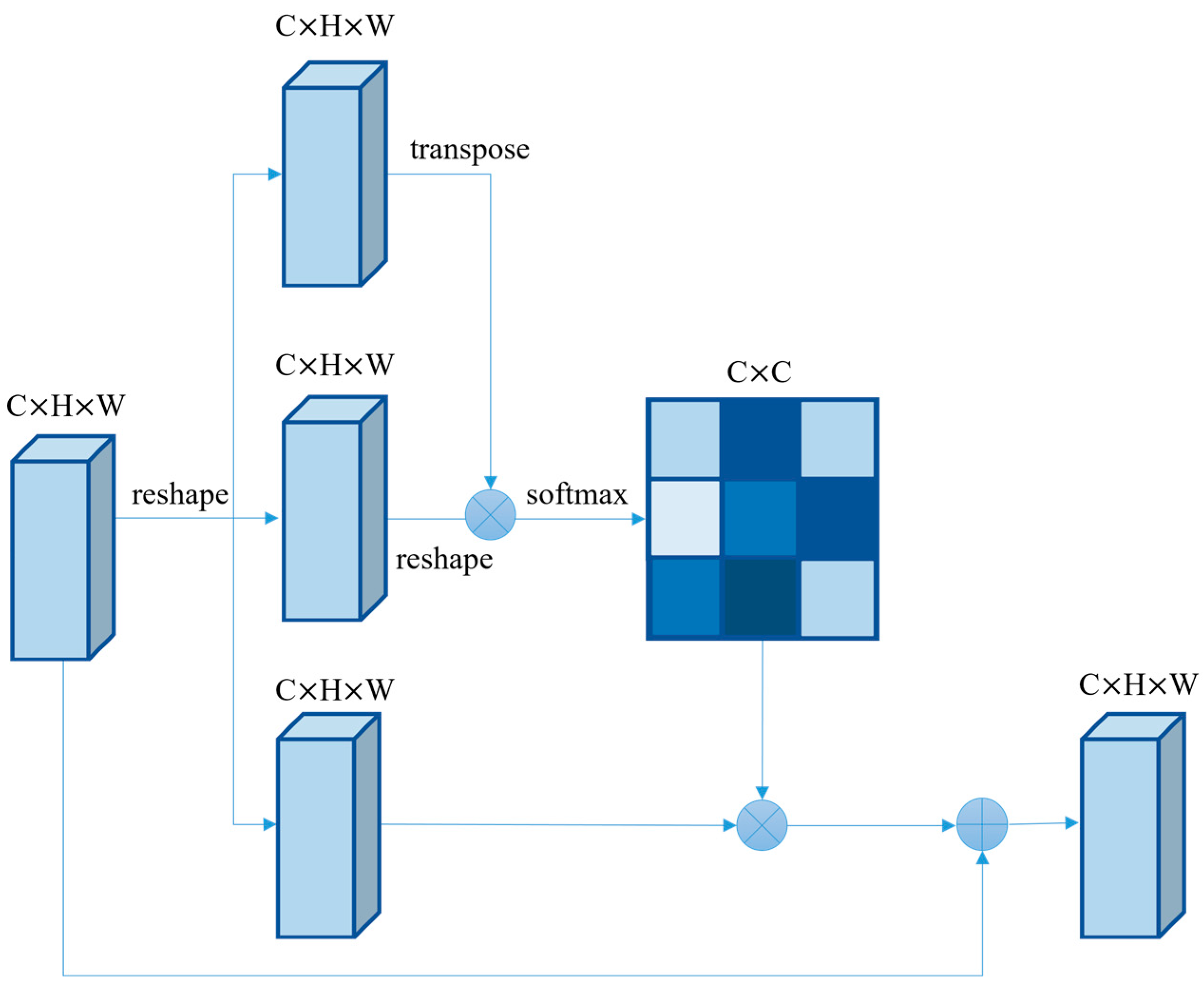
The CAM is similar in structure to the PAM, but it has a few differences. The structure of the CAM is given in
Figure 4. The first difference is that the number of channels is smaller, so there is no need to change the feature map’s shape using convolution to reduce the number of operations. The other point is that the shape of the generated attention weight map is changed, and CAM focuses on the connection between the different channels of the features. In the network structure, CAM swaps the position of the location attention module dot product, and the shape of the generated attention weight map is
, thus establishing the influence relationship between features in different channels.
The overall structure of CAM is shown in Equation (3).
where
denotes the attention probability map calculated, and
is the final output, obtained by summing the input and the optimization attention map.
refers to the size of the feature map reshape to
.
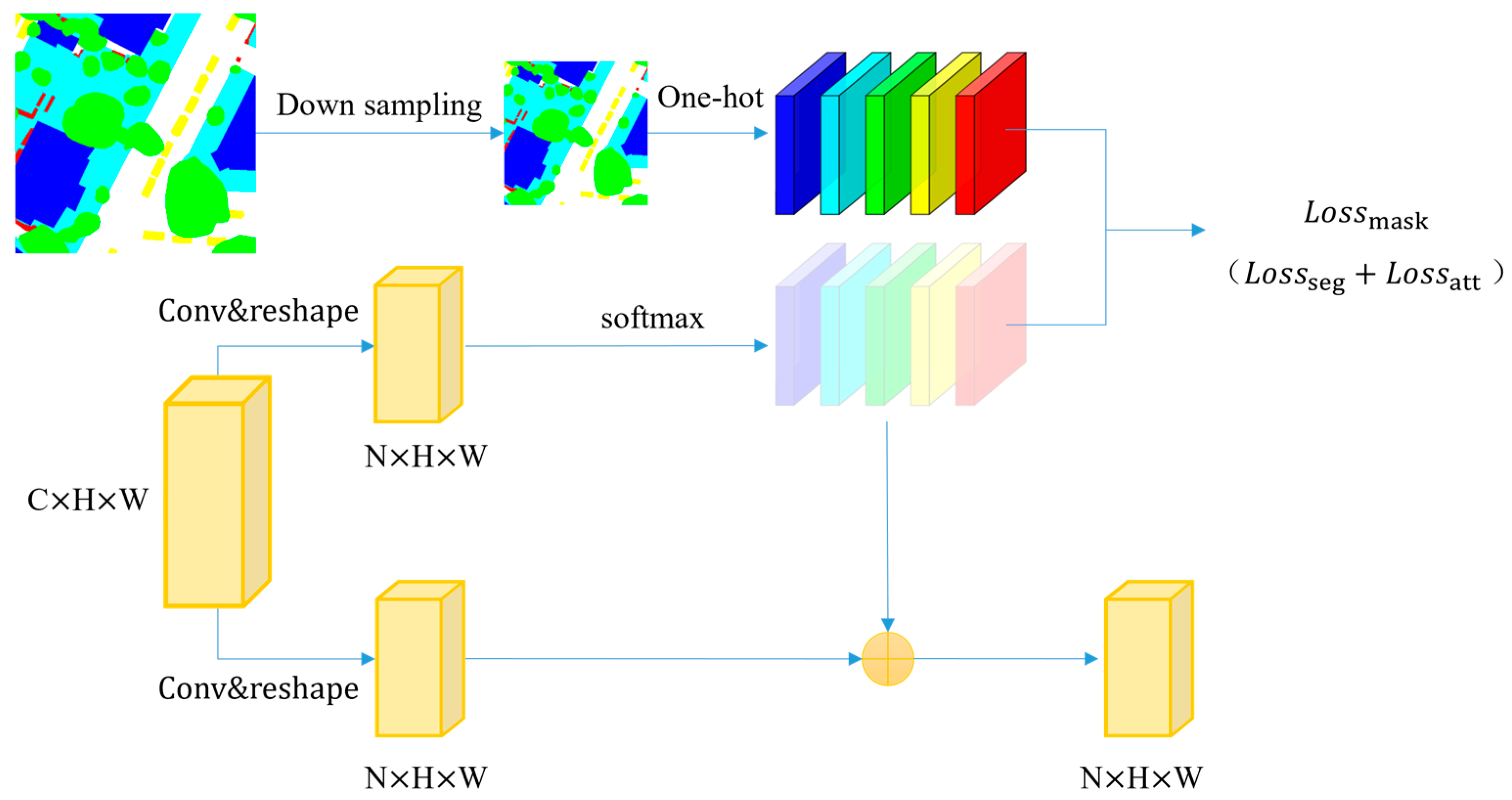
3.2. Label Attention Module (LAM)
We built a brand-new attention mechanism at different views, inspired by the effectiveness of attention-based methods. Unlike the self-attention mechanism, we use the label to generate attention probability maps. Thus, LAM can gather more global features. The structure is shown in
Figure 5.
The input (
×
×
) is turned into two parts shaped (
×
×
) by convolution and reshaping, where
is the number of classifications. LAM’s output is the weighted summation of the attention and value parts. In addition, after the SoftMax function, a loss function is computed the attention probability map and a reshaped one-hot label.
where
denotes the attention probability map, and
denotes the output features of the attention module.
The convolution neural network’s backpropagation technique parameter optimization is Equation (5). The loss function is shown in Equation (6).
where
is the learning rate, and
is the derivative of the loss function with respect to the parameters of the layer.
refers to the cross-entropy loss function.
The loss function consists of two parts: the segmentation part and the label attention part, which are, respectively, defined as , . The label attention loss helps LAM generate prediction map prototypes that facilitate the transfer of feature information.
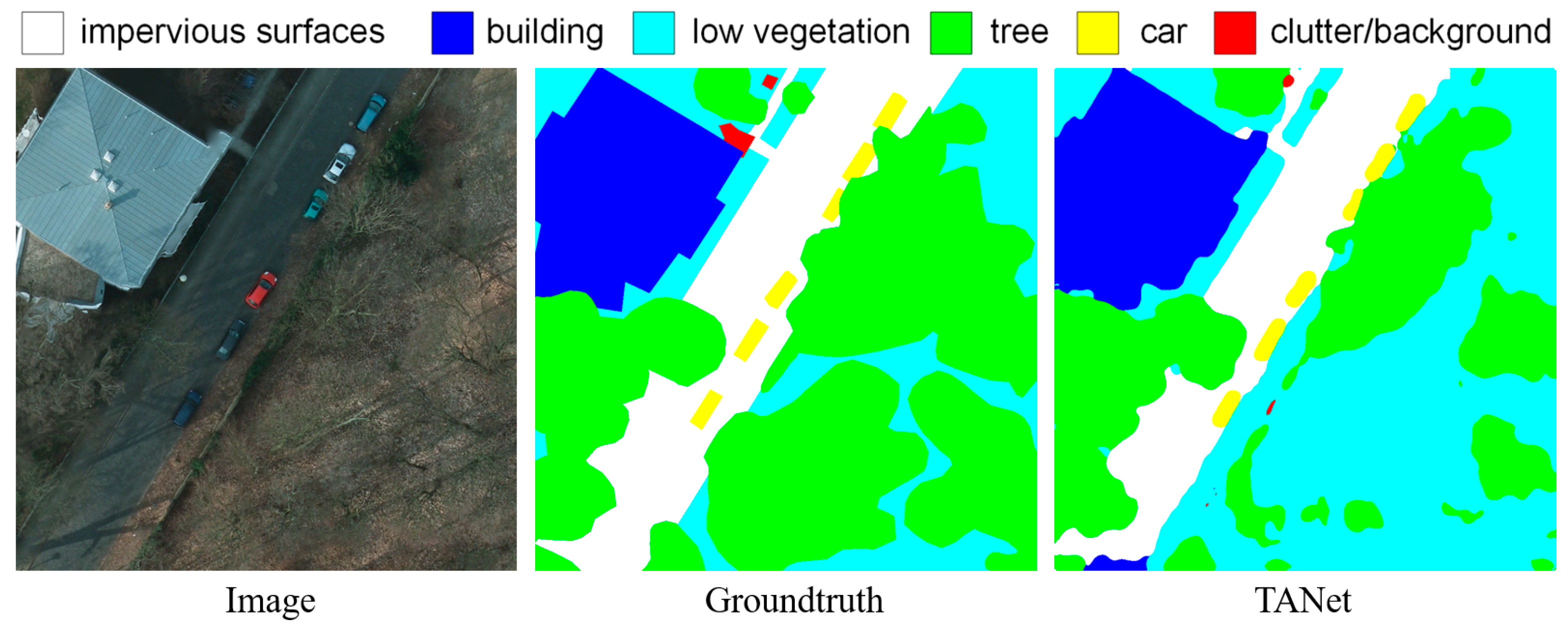
3.3. Multi-Task TANet
The attention mechanism helps improve the semantic segmentation accuracy of large objects. However, with the attention model it is difficult to distinguish some similar features. Some trees without leaves are very similar to low vegetation (
Figure 6), and even humans will misunderstand them without carefully checking. Thus, the attention module failed to distinguish the tree area.
In the traditional encoder–decoder structure, one decoder generates probability maps of multiple output results by the Softmax function in Equation (7). For each pixel, the category with the highest probability is determined as the classification result for this point.
where
denotes the input vector to the softmax function, and
C is the number of categories classified.
However, there is inter-class competition between different categories of each pixel. The sum of the probabilities of all categories is 1, and different categories share a decoder to restrict each other. If the probability of a particular point after decoding by the decoder is relatively uniform, it is easy to cause misjudgments. Three solutions are proposed to solve this problem.
The first and most straightforward idea is to change the loss function, using multiple binary-classification sigmoid cross-entropy loss instead of SoftMax cross-entropy loss. We call this model TANet with multiple losses. The loss function is shown in Equation (8).
where
denotes the output of the inference model, and
denotes the attention map of LAM.
denotes the binary cross entropy loss.
The second method is Multi-model TANet. This method is to train a semantic segmentation network for each category and combine all the binary segmentation results. It is not easy to merge the results of multiple models. Here, we use the most intuitive method to combine the predicted probability maps of multiple binary segmentation models, and each pixel takes the category with the highest probability.
Another considerable solution is introducing multi-task learning, which converts a multi-category segmentation task into multiple binary-classification segmentation tasks. We call this method Multi-task TANet. The loss function is the same as TANet with multiple losses. All categories share an encoder, and each category owns a separate decoder. As shown in
Figure 2, we use the TANet decoder mentioned above. For each pixel, we use the probability of output for each category as the confidence level and select the category with the highest confidence level as the classification result of the pixel.
For the above three methods, we have conducted experiments to find the best model.
3.4. Edge Optimization
In order to further improve the accuracy of the extracted edges, we made some targeted improvements to the model. Firstly, inspired by [
39], we add a new branch of edge extraction. The purpose of this branch is to obtain edge maps of different categories. By computing loss between the edge branch extraction edge result and the edge truth map, the edge bifurcation of the extraction results can be improved.
However, the standard semantic segmentation loss function, like cross-entropy, is unsuitable for computing edge map loss. The extraction result of the edge map may have a slight misalignment with the actual value map, and the standard loss function will produce a significant deviation. Hence, a suitable loss function for the edge map must be selected. We changed the loss function from cross entropy to
Loss [
40].
DT Loss uses distance transform (
), which transforms an edge map into a distance map. In our task, the
Loss can be represented in Equation (9).
where
denotes distance map, and
j,
k denotes the pixel coordinates.
and
represent the predicted edge map and the actual edge map.
Inspired by the distance transform method, we can transform the discrete edge map into a continuous distance map. Since the distance map already contains edge information, we can directly add a new branch to predict the distance map, and the loss function can be the common MSE.
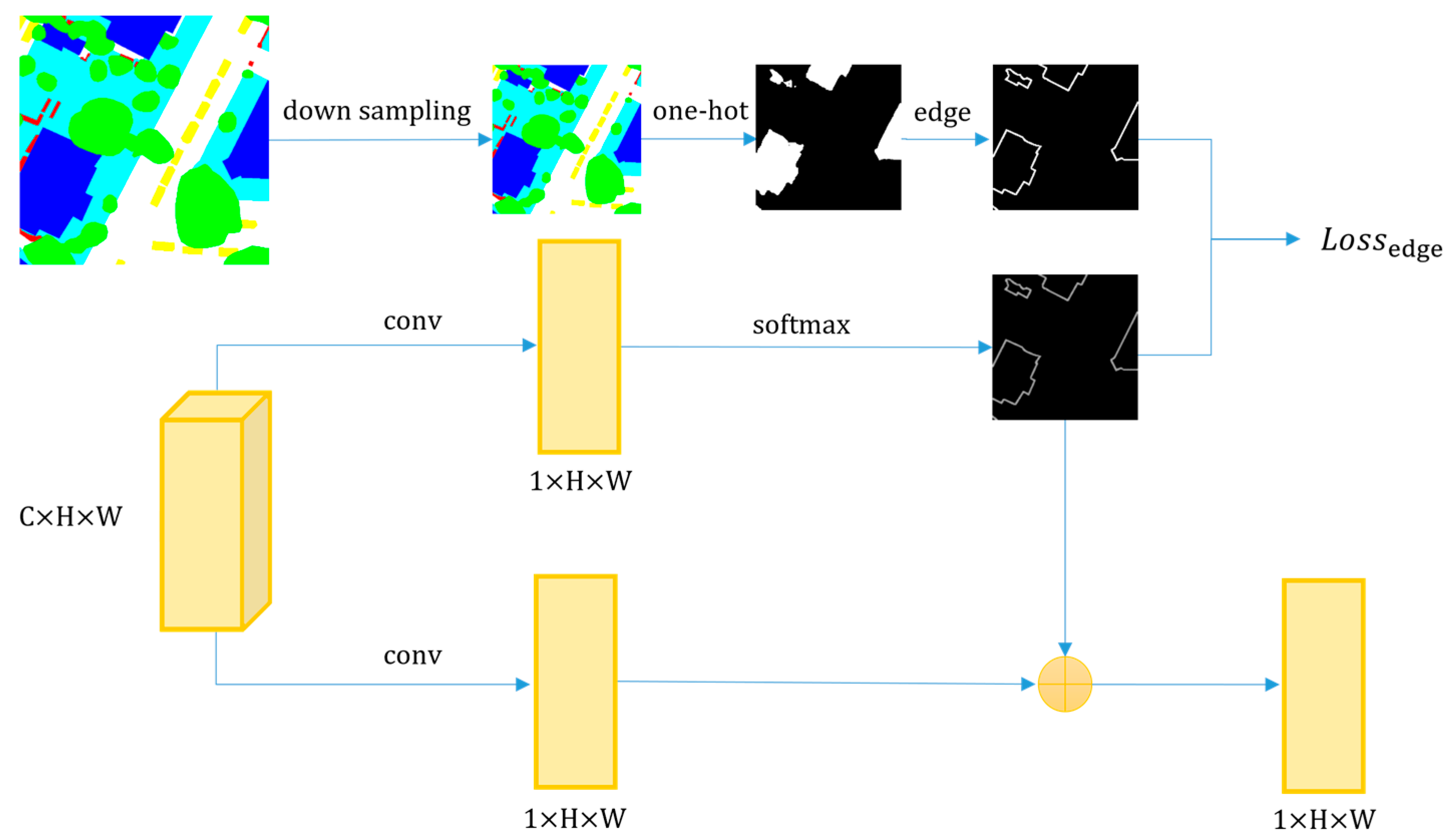
Furthermore, an edge attention module (EAM) is added to each decoder. As shown in
Figure 7, the overall architecture of EAM is consistent with of LAM, the difference is that the attention probability map used in EAM is the edge map of labels.
The loss function
is just the edge map attention part. Structure and loss of EAM is shown as follows.
where
denotes the attention probability map, and
denotes the output features of the attention module. EAM’s output is the weighted summation of the attention and value parts.
Using the boundaries of different feature categories in the labels, an edge map is drawn as the guiding information of the edge attention probability map, and the rest of the model is consistent with all the label attention modules. Since the model contains multiple decoders, each corresponding to a feature class, the edge attention module in each decoder has the same basic structure.
By combining these three improvements, the edges of the extraction results can be further improved.
3.5. Descriptions of Datasets
In order to demonstrate the effectiveness of the model, several remote sensing image semantic segmentation datasets are used in this paper. On the one hand, we use two publicly available ISPRS remote sensing image semantic segmentation datasets. On the other hand, a self-made CZ-WZ multi-category semantic segmentation dataset is used. The differences in resolution and image sensors between the two datasets are significant, so experiments on the three datasets separately can verify the model structure’s effectiveness in different data styles.
Firstly, the Potsdam 2D semantic labeling dataset [
41] contains 38 patches, each consisting of a true orthophoto (TOP) extracted from a larger TOP mosaic. The label contains six categories: impervious surfaces, buildings, low vegetation, trees, cars, and clutter/background. Four spectral bands exist in each TOP image (red, green, blue, and near-infrared), and we only use the RGB channels in this work.
The second dataset is the Vaihingen dataset [
42], which contains 33 TOP patches of different sizes. The ground sampling distance of the TOP is 9 cm. The reference data are divided into the same six categories as the Potsdam dataset. Each TOP image has three spectral bands (red, green, and near-infrared).
The third dataset is the CZ-WZ dataset. The original images come from the Changzhou area in Sichuan Province and the Wuzhen area in Zhejiang Province, China. The spatial resolution of the experimental remote sensing images is 0.51 m. Each TOP image has three spectral bands (red, green, and blue). The label is self-made and classifies the remote sensing image features into five categories: buildings, roads, vegetation, water bodies, and backgrounds.
Each training image is cut into 1024 × 1024 patches. After cutting, the Potsdam dataset contains 1176 training samples and 504 test samples; the Vaihingen dataset contains 221 training samples and 63 test samples; the CZ-WZ dataset contains 1080 training samples and 260 test samples. The training of convolution network models usually requires a large number of samples. Based on the existing dataset, this work increases the network training samples through data enhancement. The original and label images are flipped horizontally or vertically, cut at random positions, and randomly transformed HSV. Data enhancement changes the number of training samples to five times the original.
3.6. Evaluation Metrics
Following the evaluation method used in the literature [
22], we evaluate the performance of methods by three metrics: overall accuracy (
OA), per-class
F1 score, and average
F1 score.
OA is the ratio of the number of correct pixels to the total number of pixels.
F1 score for classification is calculated as the harmonic mean of precision and recall [
22].
We calculate the
F1 score for each foreground category to assess the proposed network’s performance. We also calculate the
OA for the whole dataset. The calculation formula is as follows.
with the following terms: True Positive example (
TP), False Positive Example (
FP), True Negative example (
TN), False Negative example (
FN).
4. Results and Discussion
In this section, we validate the effectiveness of the proposed attention modules and the multi-task framework. Firstly, we use UNet as our baseline and then utilize an ablation study to show the tests of the proposed triple attention modules. Then, we experimented with the three methods above to find the best model.
4.1. Ablation Study of Triple Attention Modules
The proposed TANet contains PAM, CAM, and LAM, three attention modules. PAM and CAM are self-attention modules proposed by DANet, and LAM is proposed by our paper which is a label attention module. In order to verify the effectiveness of the three attention modules, we replaced UNet’s decoder with PAM + CAM, LAM, and TANet (PAM + CAM + LAM).
4.1.1. Experiments Results on Potsdam Datasets
The attention modules focus on targets with a large area and a wide distribution range, such as buildings, low vegetation, and impervious surfaces. As shown in
Table 1, after replacing the decoder with PAM and CAM, the F1 scores of impervious surfaces increases by 0.85%, and building F1 score increases by 2.13%. As for LAM, the F1 score for building increases by 1.24% and that for tree by 0.51%. This is because TANet combines the advantages of the previous two models and thus achieves the best classification results. TANet increases F1 of impervious surfaces, buildings, low vegetation, and trees compared with UNet by 1.80%, 2.48%, 0.85%, and 0.72%, respectively. An interesting result is that UNet obtains the highest score for the segmentation result of the car. Since the attention module in this article pays more attention to large-scale and complex targets, there is no noticeable improvement for small targets such as cars.
4.1.2. Experiment Results on Vaihingen Datasets
We perform experiments on the ISPRS Vaihingen benchmark to assess TANet’s performance further. We used the same training and testing setup in the experiments on the Vaihingen dataset. As shown in
Table 2, TANet increases the F1 score of impervious surfaces, buildings, low vegetation, trees, and cars compared with UNet by 3.43%, 3.77%, 8.63%, 1.45%, and 9.15%. In this experiment, the performance of using the LAM decoder alone is closer to TANet, which means LAM played a more critical role in this model.
4.1.3. Experiments Results on CZ-WZ Datasets
We conducted experiments on CZ-WZ datasets to further evaluate the effectiveness of TANet. As shown in
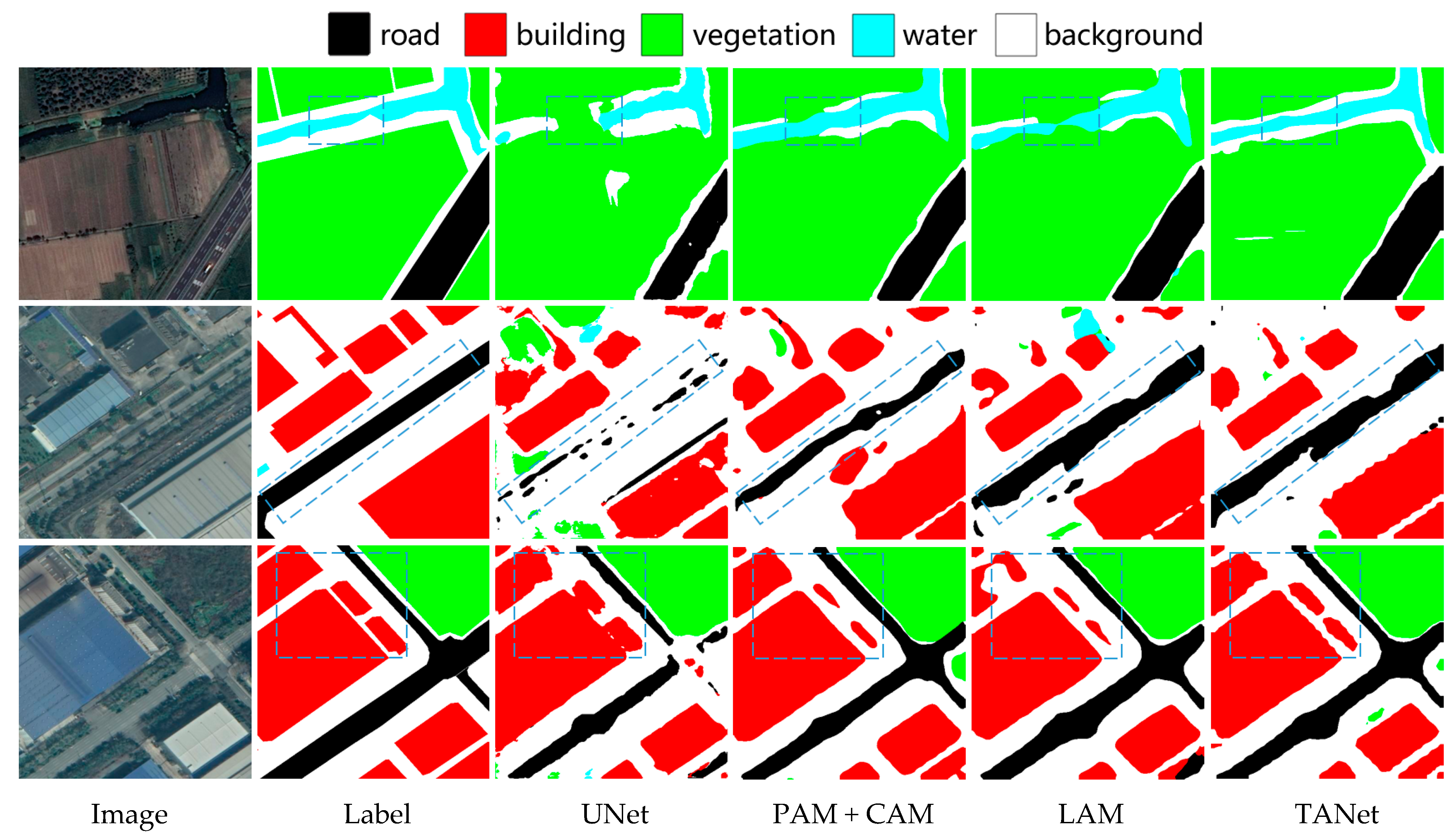
Table 3, in terms of individual category accuracy, it is evident that the improvement is excellent for roads and water bodies. Using UNet as a benchmark, the F1 scores for roads are improved by 9.16%, 12.16%, and 13.41% for PAM + CAM, LAM, and TANet, respectively. This is because UNet cannot effectively learn the global features for this type of distribution with a large range and infrequent sample occurrence, which results in lower accuracy. Moreover, after the attention mechanism is introduced, the extraction accuracy of roads is significantly improved, which shows that the global features are very effective for road extraction. Like roads, water bodies also belong to the category with a larger distribution range and lower frequency of occurrence. They are improved by 6.20%, 6.26%, and 6.59% relative to UNet, PAM + CAM, LAM, and TANet, respectively. Vegetation was also entered as a feature type with a large distribution range. However, vegetation occurred in the sample at a high frequency, so the extraction accuracy of each scheme exceeded 90%. For the vegetation category, PAM + CAM has more improvement than LAM, while LAM has more improvement on roads and water bodies. The two schemes have some overlapping parts for the overall accuracy improvement. However, there are still differences in different categories, combining the advantages of TANet and fusing the two to obtain optimal accuracy.
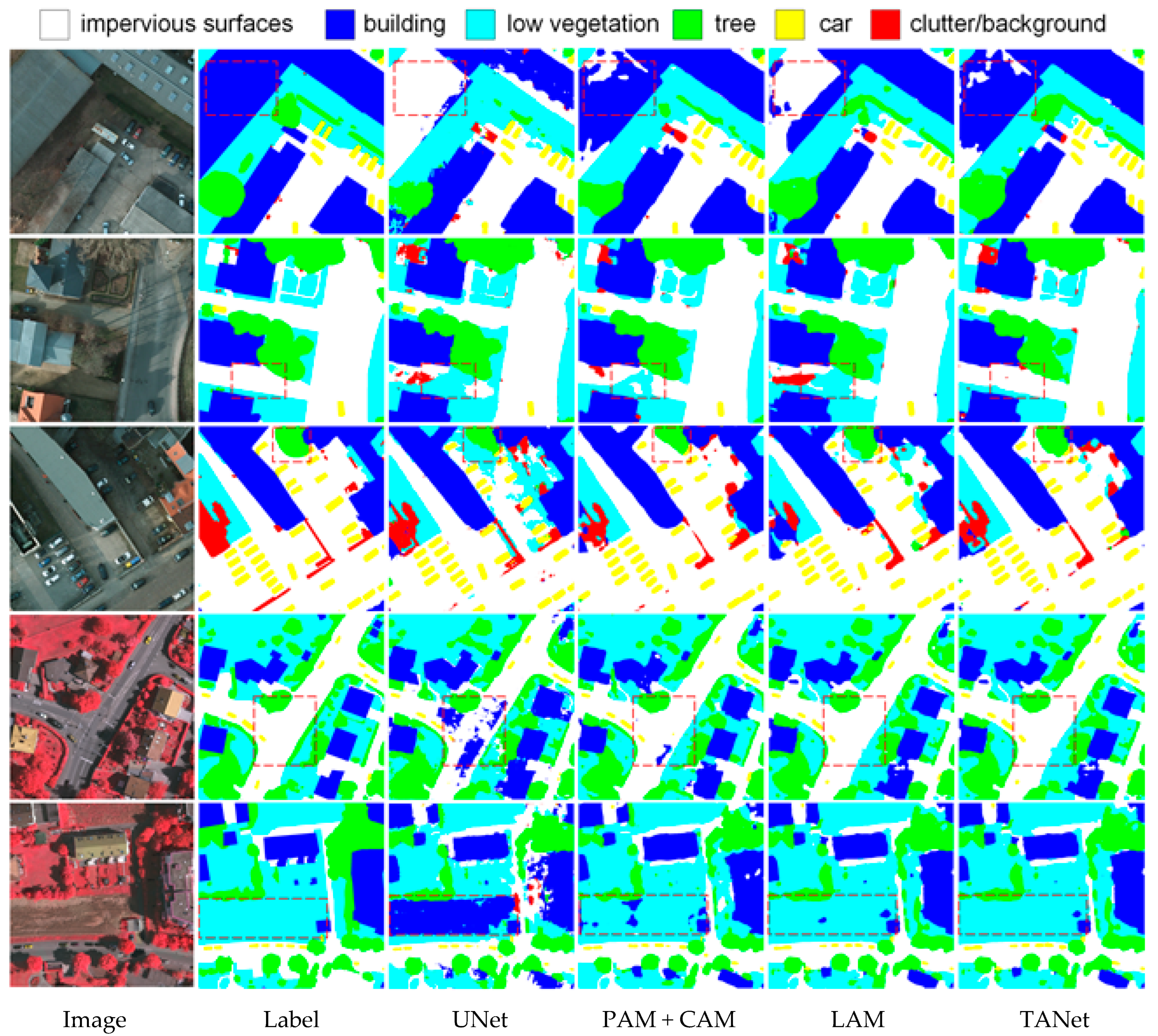
We compare the results before using the proposed module and after in
Figure 8 and
Figure 9. It can be clearly observed that the ability to recognize a wide range of object types is enhanced after combining the attention module. For example, in the second row in
Figure 8, part of the impervious surface area is covered by shadows. TANet recognizes the impervious surfaces correctly after the global features introduced by the attention module’s introduction.
4.2. Visualization of LAM
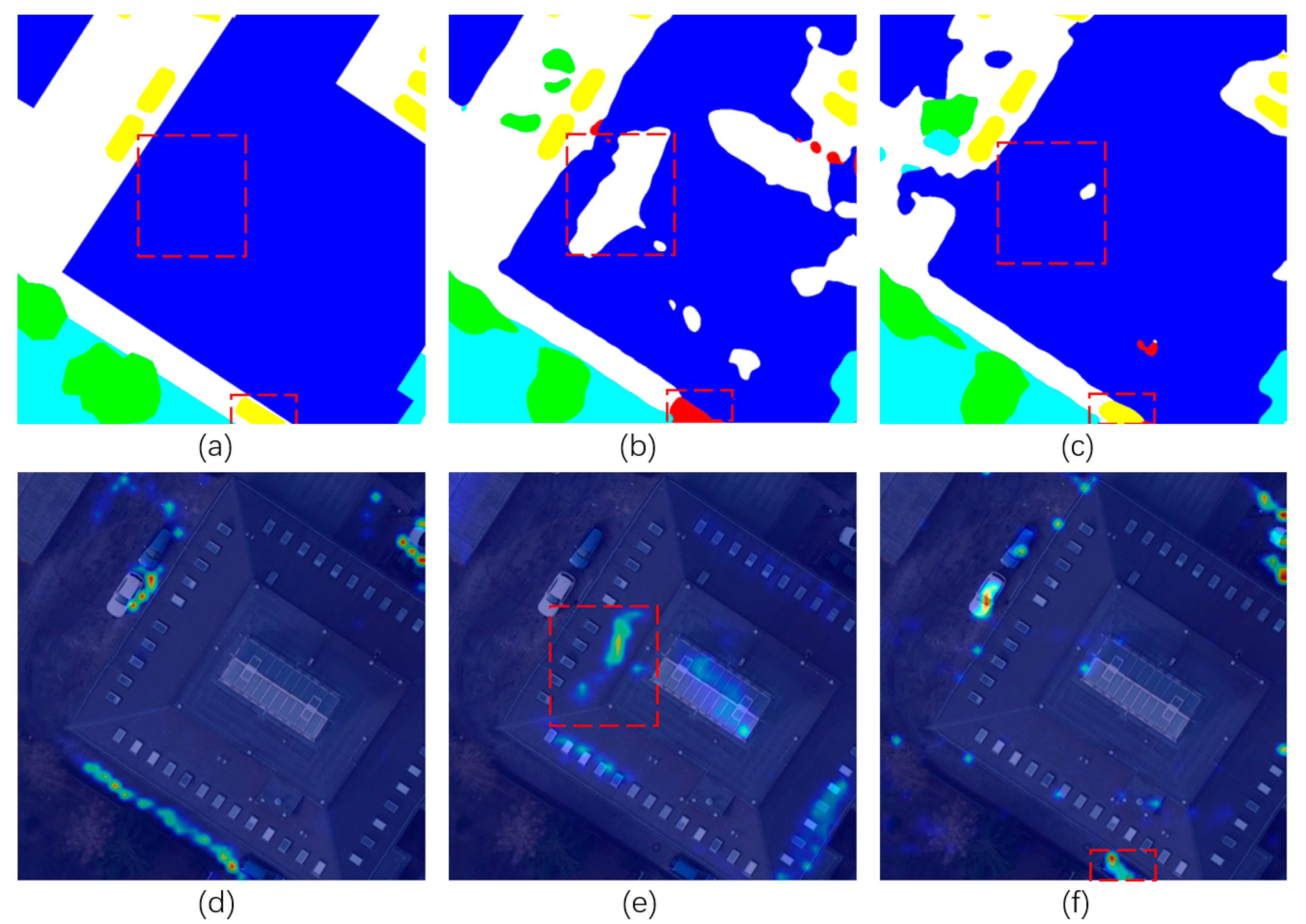
We visualize attention maps in LAM to better understand our attention modules. The number of channels of attention maps generated by LAM is the same as the number of segmentation categories, and we overlay the results of each category of the attention map on the original image.
Figure 10 shows the attention map results of impervious surfaces, buildings, and cars. The feature response extracted by the attention modules is similar to the segmentation result. Moreover, attention maps of LAM have made some corrections to PAM and CAM extraction results. In the red rectangle, the segmentation results of PAM and CAM are wrong, and with the help of the LAM’s attention map, TANet obtains the correct recognition result.
4.3. Ablation Study of Multi-Task Learning
After the introduction of the attention module, the segmentation accuracy of a wide range of targets was improved. Observing the extraction results of the TANet model, it is found that there are still some misjudgments of similar features. We conducted several experiments to solve this problem according to the ideas proposed in
Section 3.3.
- (1)
TANet with multiple losses
We use binary cross-entropy loss for each category instead of softmax cross-entropy loss.
- (2)
Multi-model TANet
For each category, we trained an individual network. For each input image, we fused the output probability maps of each category to obtain the final output result.
- (3)
Multi-task TANet
We convert a multi-category segmentation task into multiple binary-classification segmentation tasks. All tasks share one encoder, and each task owns an individual decoder.
4.3.1. Experiment Results on Potsdam Datasets
As shown in
Table 4, Multi-task TANet improves the performance remarkably. Compared with the baseline UNet, they employ a multi-task decoder yielding 88.35% in OA, which brings a 2.87% improvement. The results show that the accuracy can only be improved slightly if the loss function is replaced without increasing the number of decoders. Since all categories share one decoder, and the characteristics of different categories are quite different, it is difficult for one decoder to summarize the global characteristics of all categories. Another finding is that the fusion results of multiple binary segmentation models are poor. Since the models are trained separately, merging the results of multiple models is not an easy task.
4.3.2. Experiment Results on Vaihingen Dataset
Table 5 reports the quantitative results of the Vaihingen datasets. Compared with the baseline UNet, the methods that combine multi-task ideas achieved higher accuracy. Similar to the performance of the Potsdam dataset, changing the loss function does not significantly improve the model. However, the multi-model fusion performed better on the Vaihingen dataset, especially the tree and car categories, which achieved the highest F1 scores. The performance of multi-model TANet is not stable in different datasets. In terms of large-area features, Multi-task TANet achieved better results. Similar categories are easier to distinguish under the action of multiple decoders.
4.3.3. Experiment Results on CZ-WZ Dataset
As shown in
Table 6, multi-task TANet significantly improves the performance of image semantic segmentation. Compared to UNet, TANet with multiple losses, Multi-model TANet, and Multi-task TANet improved 5.27%, 5.00%, and 8.04% in F1 score, and 2.14%, 1.88%, and 3.39% in OA score, respectively. Compared to TANet, the extraction accuracy of Multi-loss TANet and Multi-model TANet decreased, and Multi-task TANet achieved the highest accuracy. Different multitasking strategies have different effects on the model. TANet with multiple loss only uses the multitasking loss function without changing the model structure. The model still has parameter competition, and it is still difficult to avoid the problem of misclassification of similar categories. The multi-model strategy used by Multi-model TANet has higher extraction accuracy in a single model. However, it is more difficult to fuse the multi-category results. The method of directly taking the most significant term of probability value does not completely merge the multi-category results, which is caused by the differences in the predicted probability values of different models, so the multitask approach of the multi-model strategy has some instability.
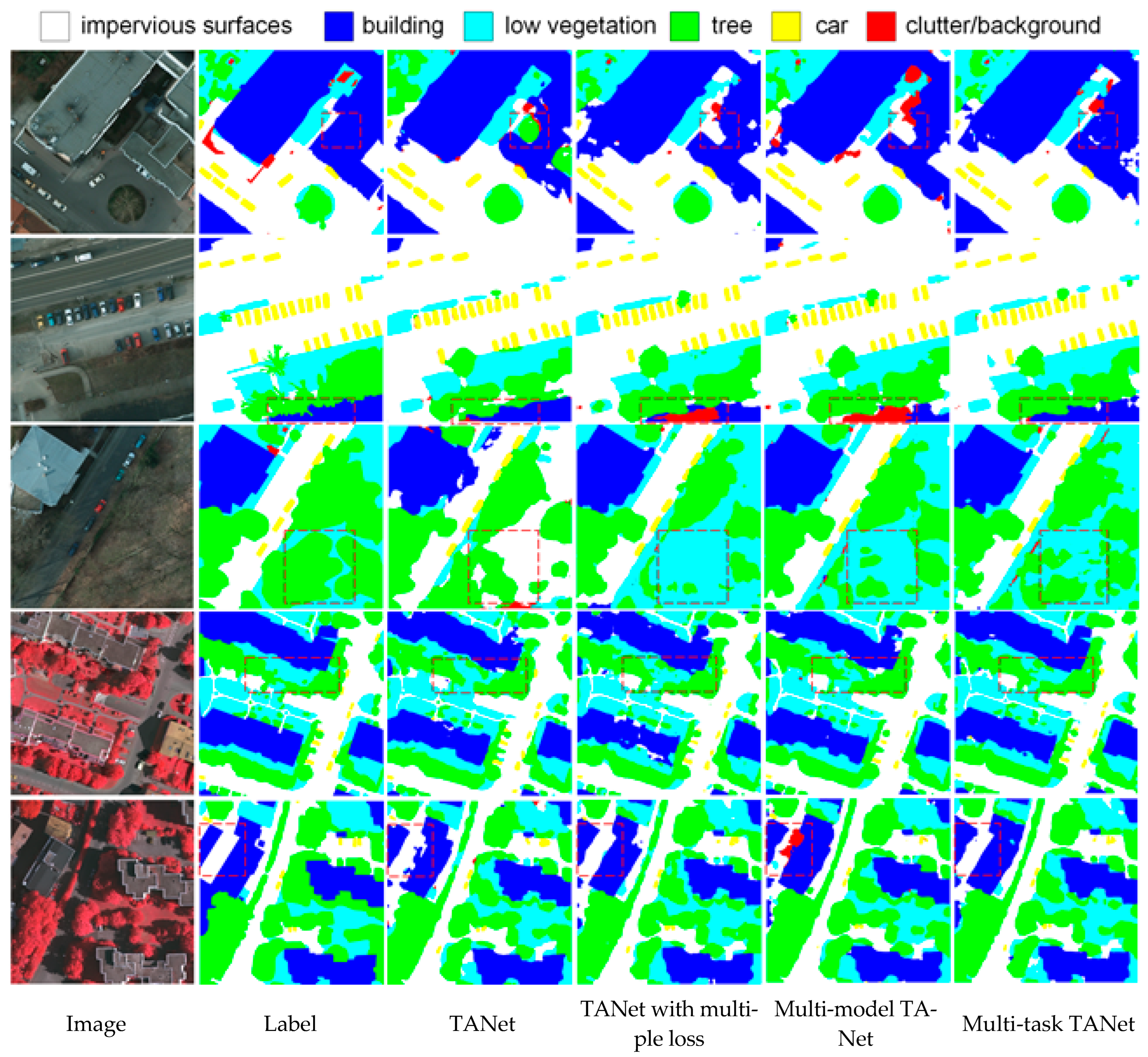
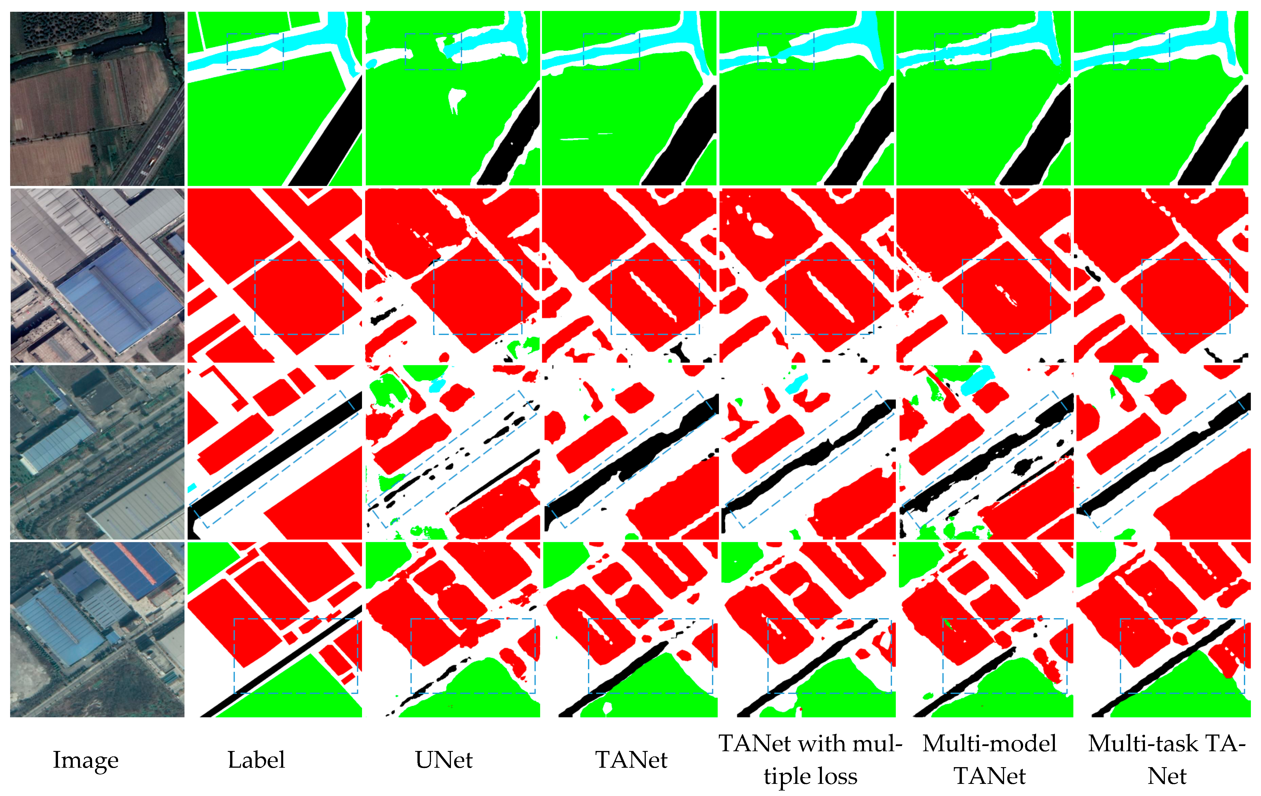
Figure 11 and
Figure 12 compare the segmented results on different approaches to multitasking ideas. The multi-task mechanism focuses on solving the problem of misidentification of similar features. Multi-task TANet with multiple decoders achieved the best results. Since each category has a dedicated decoder, each decoder is more focused, thereby improving the ability of category discrimination.
4.4. Edge Optimization Results and Discussion
The optimization includes the edge map branch (EB), the distance map branch (DB), and EAM. Firstly, to prove the validity of the DT Loss, we introduce the edge map branch and compare the results using DT Loss and cross-entropy (CE). In
Table 7, EB_DT denotes the edge map branch with DT Loss, and EB_CE denotes the edge map branch with CE Loss. According to
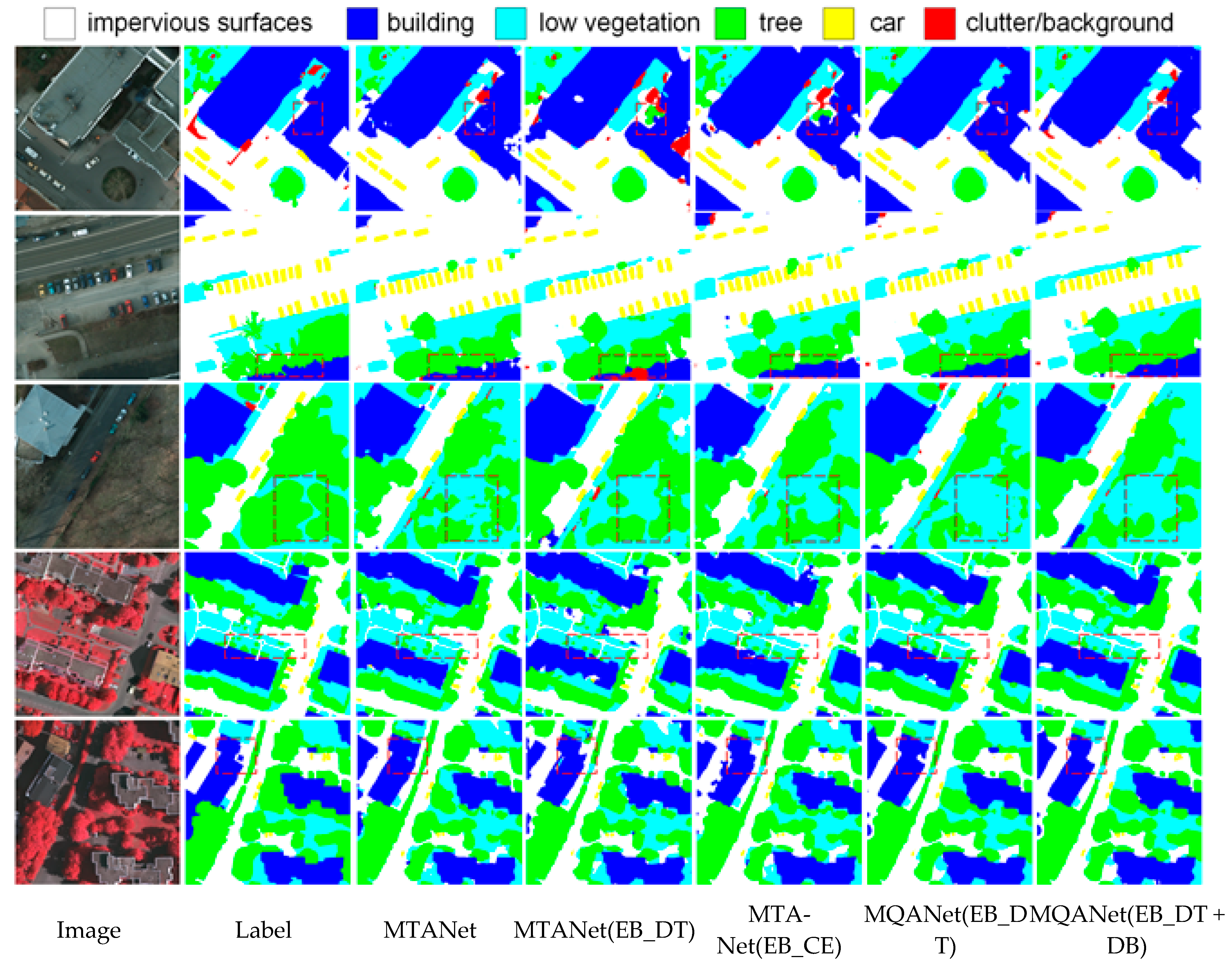
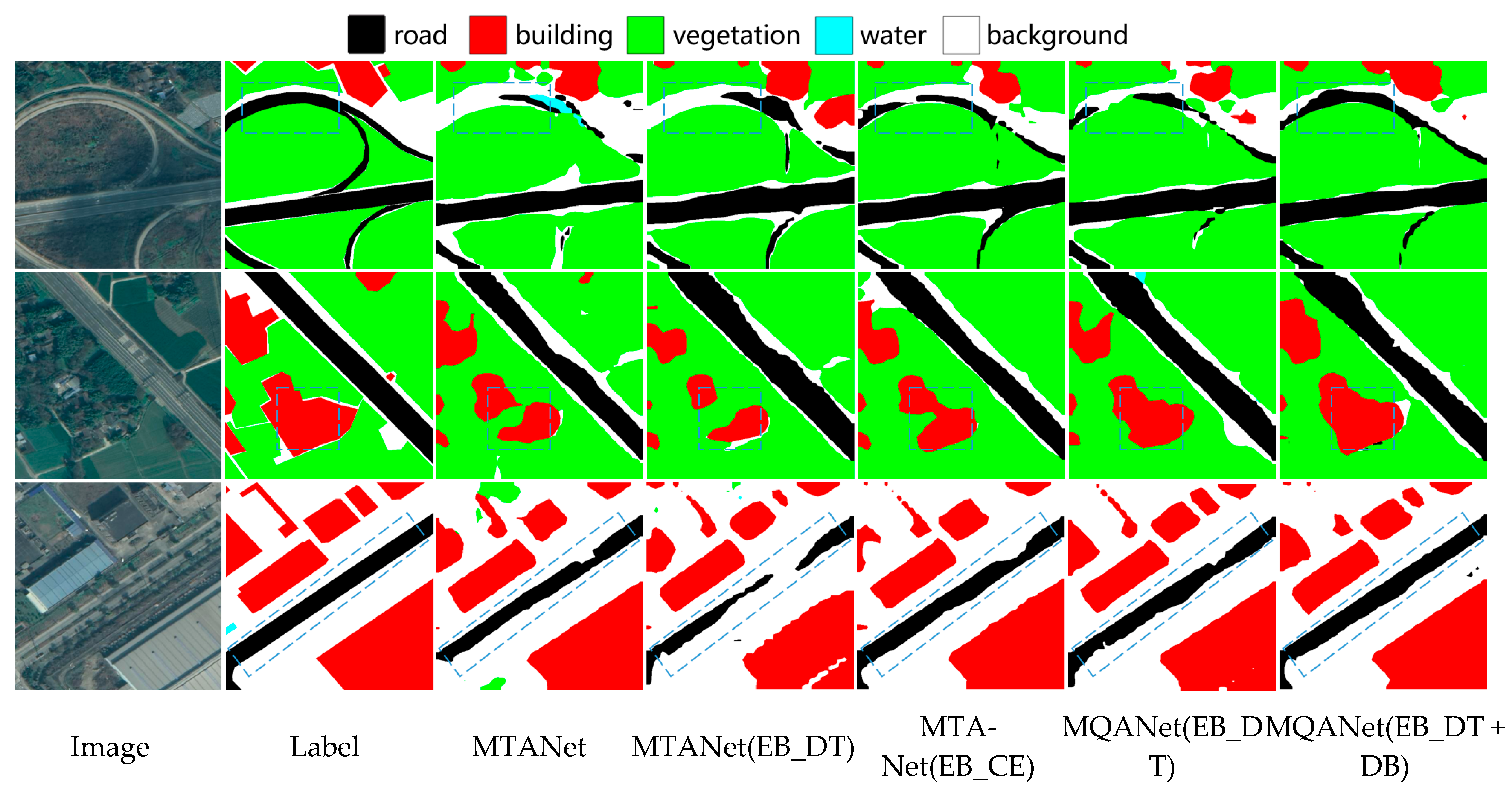
Table 7, the results of different modules of edge optimization on three datasets can be obtained, and the edge optimization of EB_DT and DB is the best result in MQANet.
Then we evaluate the effects of the proposed distance branch and EAM. In
Table 7, DB denotes the distance branch. MQANet means the previous MTANet combined with edge attention to form a Multi-task Quadruple Attention Network.
Table 7 shows that all three modules have improved the segmentation results. In
Table 7, MTANet is Multi-mask TANet, and MQANet is Multi-mask QANet.
The two datasets from Potsdam and Vaihingen were applied to tests for Unet, TANet, and Multi-task QANet. The results are shown in
Figure 13 and
Figure 14. Compared with the three test datasets, the segmentation results of Multi-task QANet present a better effect than Multi-task TANet. The modules, the first line of
Figure 13, can clearly show the performance, especially for the edge contour of the target.
Table 7 shows that after optimization of each module of edge extraction, the overall accuracy of the model is improved to a certain extent, and compared with MTANet (EB_CE), MQANet (EB_DT + DB) shows an improvement of 0.61% and 0.49% in F1 score and OA, respectively. The slight improvement since the edge part accounts for a smaller proportion of the total image area. The optimized edge extraction accuracy contributes less to the overall accuracy improvement. From the results of MTANet (EB_DT) and MQANet (EB_DT), it can be seen that different edge extraction loss functions significantly impact the overall accuracy, and using the cross-entropy loss function to extract edges even reduces the original model accuracy. Moreover, the distance transform loss function can be better applied to the edge extraction task. The results of MQANet (EB_DT + DB) show that the newly introduced distance transform branch and edge attention module can both help to improve the accuracy.
4.5. Discussion of Overall Experimental Results
Table 8 is presented to analyze the results of our methods based on the two public datasets. The Mean F1 and OA of the surface objects have been promoted for the two datasets. For the Potsdam dataset, the 2.83% Mean F1 and 3.57% OA of MQANet are higher than those of Unet. For the Vaihingen dataset, the 7.05% Mean F1 and 6.33% OA of MQANet are higher than Unet.
In addition, we tested the execution time of our proposed networks and Unet based on the method provided by Dong et al. [
43], and the test results is the right column in
Table 8. The test method sets the batch size to 1 and lets the network predict 200 images, the final execution time is the average of the total running time. That is the execution time of the network for a single image. From
Table 8, it can be seen that the execution time of each image is reduced 66.6 ms compared to UNet, and the execution time of UNet is more than doubled compared to MQANet. Because our proposed multi-tasking mechanism splits a multi-category segmentation task into several binary-classification segmentation tasks, it can effectively reduce execution time and achieve better performance than the UNet baseline.
The experiment’s results demonstrate that MQANet obtains optimal accuracy on two public datasets of ISPRS. Our module introduces two attention mechanisms: self-attention and label-attention. Thus, we achieve an enhanced overall accuracy compared to the standard self-attention model. In addition, this paper uses a multi-decoder model to reduce the parameter competition among different classes and performs additional optimization for the edge regions, thus achieving optimal accuracy.
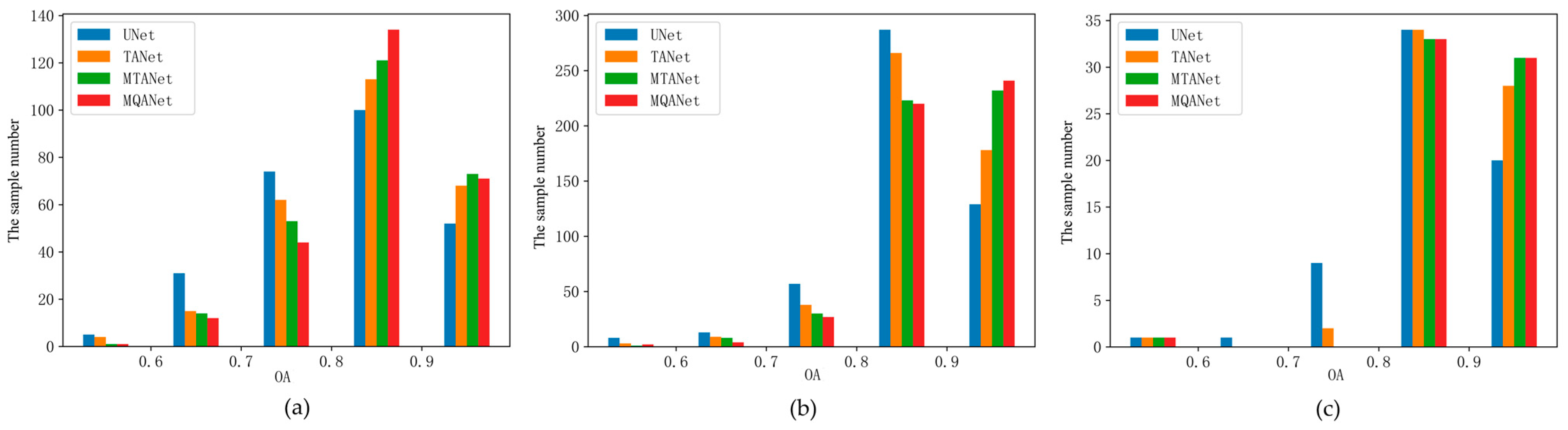
To further describe the model accuracy distribution of different datasets, we count the sample number of each model in different accuracy intervals. We use overall accuracy (OA) as the accuracy evaluation index to draw histograms, as shown in
Figure 15.
As shown in
Figure 15, in the Chongzhou–Wuzhen dataset (CZ-WZ dataset), when OA is below 0.8, the number of samples in UNet is significantly higher than that of other models. TANet, MTANet, and MQANet show a decreasing trend. In contrast, when the accuracy is above 0.8, MQANet has the largest number of samples. The above results show that MQANet achieved optimal accuracy in most samples of the CZ-WZ dataset. In the Potsdam and Vaihingen datasets, the regularities are similar to those in the CZ-WZ dataset. When the accuracy is above 0.9, the number of samples of UNet is significantly lower than that of other models, and MQANet has the largest number of samples. This indicates that MQANet also achieves the optimal accuracy in most samples of Potsdam and Vaihingen datasets.
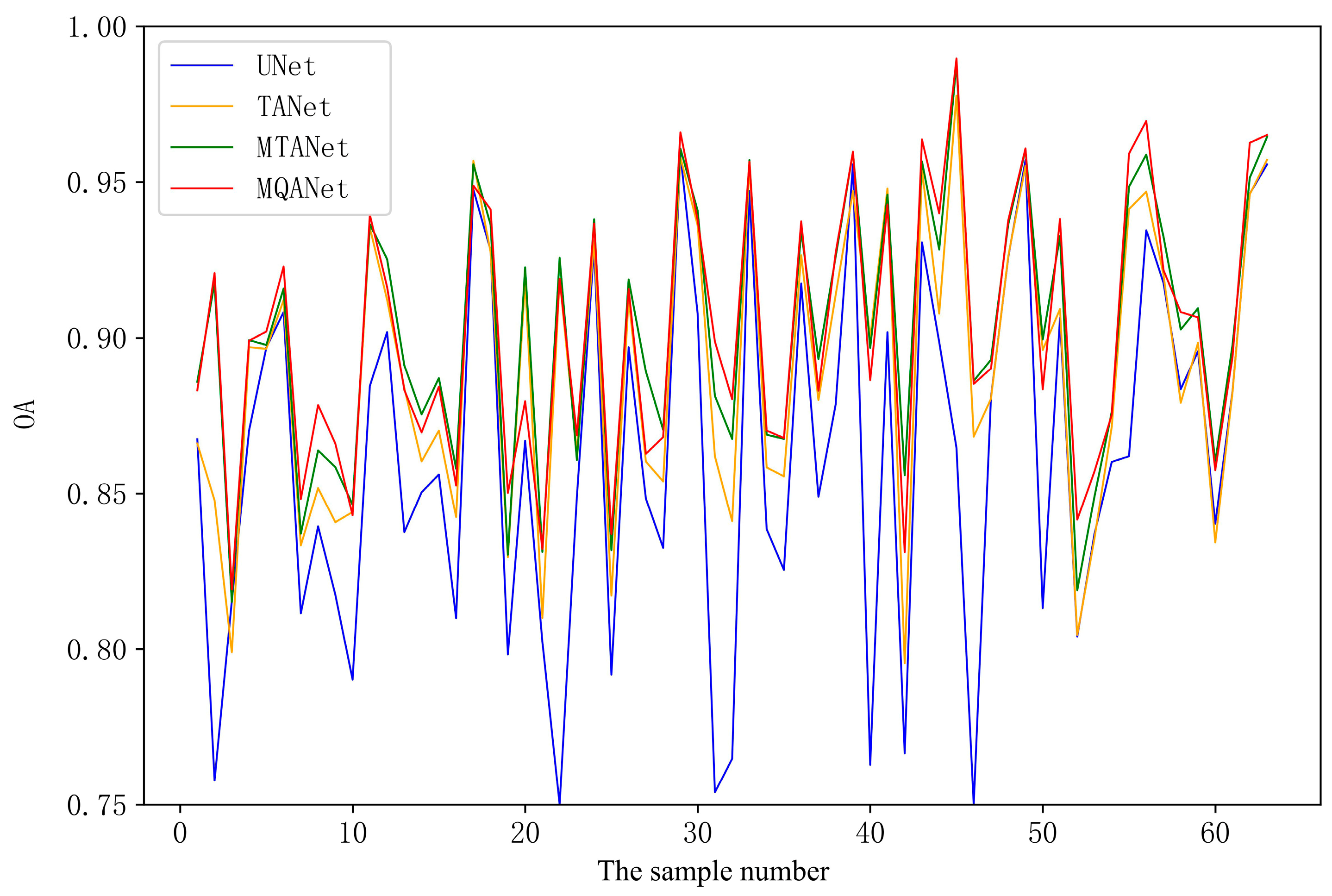
To obtain a more detailed sample distribution, we plotted the extraction accuracy of each sample as a broken line diagram in the ISPRS-Vaihingen test dataset. As shown in
Figure 16, the extraction results of MQANet are the highest in four models. TANet, MTANet, and MQANet show an upward trend in the Vaihingen test sample, which further indicates that the proposed model has a high OA index in the Vaihingen test dataset.
In addition, we compared the current work on two publicly available datasets to verify the effectiveness of our optimal model, MQANet, still using two evaluation metrics, the average F1 and OA. Among the existing works compared with this paper, the work CBAMNet [
21] containing the self-attentive mechanism, SENet [
44], and the latest network Deeplabv3+ [
11] with the spatial feature pyramid structure are included, in addition to the latest CRMS [
45] network with optimal feature extraction using the multiscale residual module. The experimental results are shown in
Table 9. As can be seen from
Table 9, the results of our proposed model MQANet show better results on both datasets. On the Vaihingen dataset, our MQANet network has higher Mean F1 and OA than other networks, and on the Potsdam dataset, our MQANet network has higher Mean F1 than other networks, and only OA is 0.08% lower than DSPCANet [
15]. Mean F1 score for classification is calculated as the harmonic mean of precision and recall [
22], and OA is the ratio of the number of correct pixels to the total number of pixels. This shows that our MQANet has certain advantages in the equalization of various objects identification.
5. Conclusions
A Multi-task Quadruple Attention Network (MQANet) is proposed to improve the accuracy of multi-object semantic segmentation of remote sensing images. We introduce the attention mechanism to obtain more global features and improve the accuracy of the large object area. Furthermore, two self-attention modules are introduced, which are named PAM + CAM, and the OA and Mean F1 are improved. Then, we build a label attention module (LAM) and combine all three attention modules into a triple attention network (TANet). Meanwhile, we proposed three alternative methods to improve the ability to identify similar objects: Multi-task TANet (MTANet). Experiment results show that the multi-task learning method obtains the highest accuracy. Finally, some edge optimizations are made to improve the accuracy of the edge area further, and we combine Multi-task TANet and edge optimizations as the Multi-task QANet (MQANet).
Three datasets were used to verify the accuracy of the proposed model. Compared with the baseline UNet in the Vaihingen dataset, MQANet improved the OA and Mean F1 by 6.33% and 7.05%, respectively. MTANet improved the OA and Mean F1 by 5.48% and 6.84%, respectively. Compared with the baseline UNet in the Potsdam dataset, MQANet improved the OA and Mean F1 by 3.57% and 2.83%, respectively. MTANet improved the OA and Mean F1 by 2.87% and 2.02%, respectively. Compared with the baseline UNet in the CZ-WZ dataset, MQANet improved the OA and Mean F1 by 3.88% and 8.65%, respectively. MTANet improved the OA and Mean F1 by 3.39% and 8.04%, respectively. Through extensive experiments, the proposed MQANet outperforms other methods by a large margin on Vaihingen, Potsdam and self-annotated datasets (CZ-WZ dataset). The results demonstrate that the proposed model (MQANet) has a large accuracy improvement in both F1 and OA indices, and the quadruple attention modules are helpful for large object semantic segmentation of RS images.
The proposed multi-tasking mechanism splits a multi-category segmentation task into several binary-classification segmentation tasks, each of which requires a separate decoder. The types of multi-object semantic segmentation involve 5 or 6 categories in our study, which can achieve better results. However, if the objects are subdivided into dozens or even more categories, the model needs to construct a decoder for each category. A large number of decoders may cause the size expansion of the model, and the applicability of the model may be decreased. In the future, more types of multi-object will be tested to optimize a more robust multi-task semantic segmentation.


 ,
, 


