Inversion of Glacier 3D Displacement from Sentinel-1 and Landsat 8 Images Based on Variance Component Estimation: A Case Study in Shishapangma Peak, Tibet, China

Abstract

Offset tracking technology is widely studied to evaluate glacier surface displacements. However, few studies have used a cross-platform to this end. In this study, two heterogeneous data sources, Sentinel-1 and Landsat 8, from January 2019 to January 2021, were used to estimate the offset, and then the optimal estimation of the 3D deformation rate of a Himalayan glacier was obtained based on the joint model of variance component estimation. The results show that the maximum deformation rates of the glacier in the east–west direction, north–south direction, and vertical direction are 85, 126, and 88 mm/day, respectively. The results of the joint model were compared and analyzed with the results of simultaneous optical image pixel offset tracking. The results showed that the accuracy of the joint solution model increased by 41% in the east–west direction and 36% in the south–north direction. The regional flow velocity of the moraine glacier after the joint solution was consistent with the vector boundary of the glacier cataloging data. The time-series results of the glacier displacement were calculated using more images. These results indicate that the joint solution model is feasible for calculating temporal glacier velocity. The model can improve the time resolution of the monitoring results and obtain further information on glacier characteristics. Our results show that the glacier velocity is affected by local terrain slope and temperature. However, there is no absolute positive correlation between glacier velocity and slope. This study provides a reference for the joint acquisition of large-scale three-dimensional displacement of glaciers using multi-source remote sensing data and provides support for the identification and early warning of glacier disasters.

1. Introduction

Under the influence of global warming, glacier melting has intensified the occurrence of natural disasters, such as landslides, mudslides, and glacial lake collapses [1]. As an important characteristic of glacier change, glacier surface displacement can reveal mass balance changes and is beneficial for the early identification of potential glacier disasters [2]. Therefore, high-precision and multi-dimensional monitoring of glacier velocity changes can provide a theoretical basis for the early warning of glacier disasters and climate analysis.

Offset tracking technology has been widely used in glacier displacement monitoring [3], with the synthetic-aperture radar (SAR) offset [4] and optical offset techniques [5] being two commonly used techniques. SAR images are not affected by weather conditions, the revisit cycle of the SAR satellite is short, and the coverage area of the SAR image is large [6]. Therefore, many scholars have estimated glacier displacement based on intensity information from SAR images [7]. For example, glacier velocity changes in Greenland from 2015 to 2017 were obtained based on Sentinel-1A SAR images [8]. The three-dimensional velocity of the Southern Inylchek Glacier as obtained from TerraSAR-X SAR data using time-series SAR offset technology [9]. However, the SAR offset tracking estimation results are ranges and azimuth offsets based on the image coordinate system. Therefore, some scholars have chosen to focus on pixel offset tracking technology based on optical images to obtain the displacement in the east–west and south–north directions [10]. For example, the mountain glacier velocity field in the Alps was calculated based on SPOT-5 optical images [11]. The 28-year landslide deformation in Peru was calculated based on sentinel-2, SPOT1-5, and Pleiades [12]. Therefore, it is common to use a single data source to carry out glacier displacement monitoring.

Joint monitoring methods have also been developed for glacial displacement monitoring of large gradient, multi-source, and multi-platform images. For example, two- or three-dimensional glacier motion monitoring is integrated with InSAR ascending and descending orbit technology [13]. The pixel-offset small-baseline subset (PO-SBAS) [14] and multiple aperture interferometry (MAI) techniques combined with multiple tracks have been used to evaluate the 3D deformation of glaciers [15]. In the joint monitoring of different platforms and different methods, the variance component estimation is the main applied model. For example, Hu et al. [16] extracted the 3D deformation field related to the Mw 7.8 earthquake in Kaiköura, New Zealand, from the SAR data obtained from the descending orbit of ALOS-2 and the ascending orbit of Sentinel-1 based on pixel offset tracking technology. In particular, the variance component estimation algorithm was used to determine the accurate weight of heterogeneous InSAR measurements. Liu et al. [17] calculated the velocity in the line-of-sight (LOS) direction by combining DInSAR and offset-tracking technology with ascending and descending Sentinel-1 images of the Urumqi Glacier No. 1 from 2016 to 2017. Meanwhile, the velocity in the azimuthal direction was obtained by combining MAI and offset-tracking technology. Then, the eastward, northward, and upward flow velocities were retrieved using the Helmert variance component estimation method. However, few studies have performed the high-precision and multi-dimensional monitoring of large gradient deformations by fusing SAR offset and optical offset based on variance component estimation. In this study, a glacier on Shishapangma Peak in the central Himalayas was evaluated using two different data sources, Sentinel-1 and Landsat 8. The optimal estimation of the 3D deformation rate of the glacier was calculated based on the variance component estimation. Finally, the calculated results were compared with the optical time-series results, and their accuracy was evaluated. The findings presented in this study provide a reference for the joint acquisition of large-gradient 3D displacement of glaciers using multi-source remote sensing data.

2. Experimental Area and Data

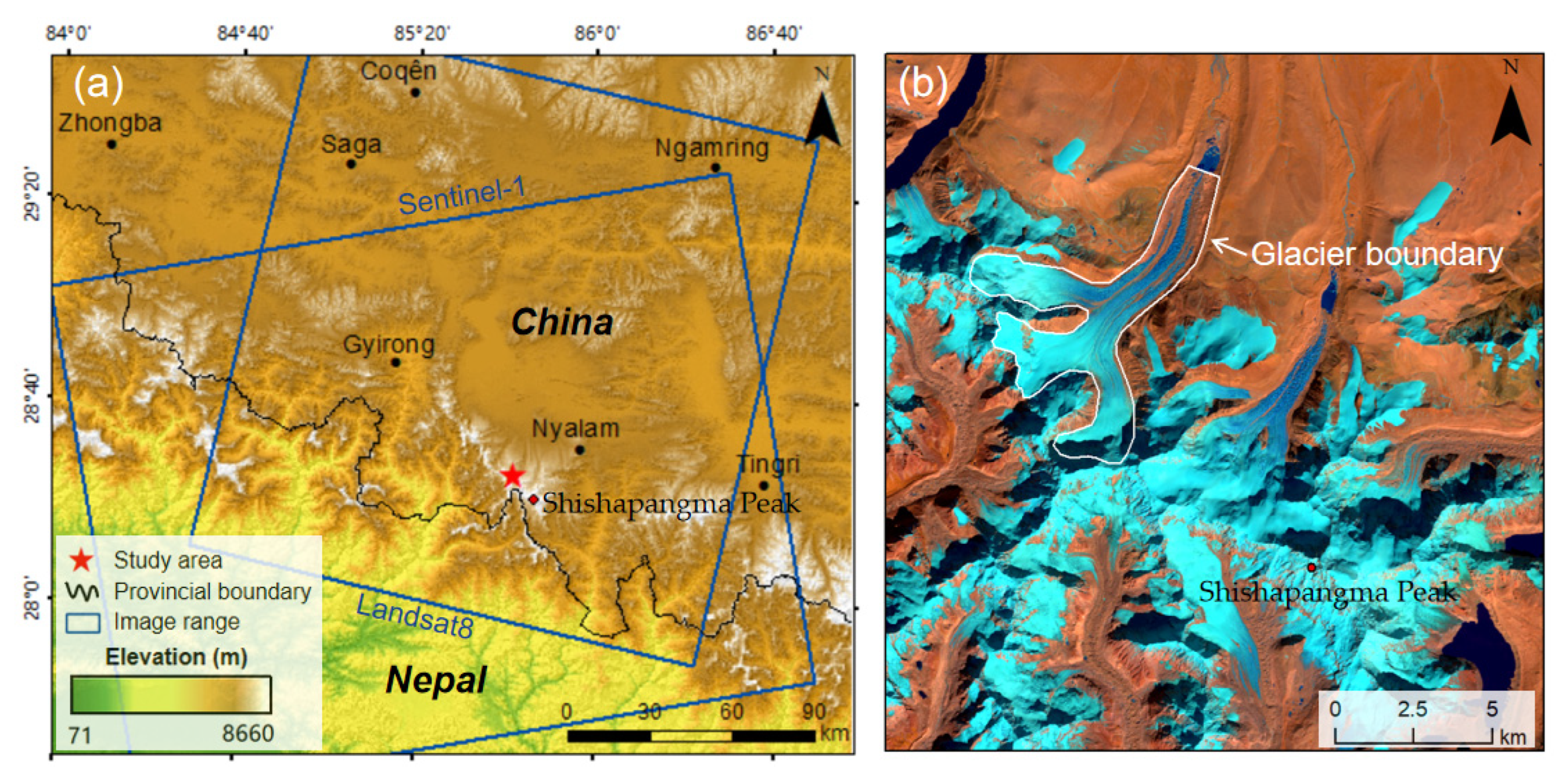
2.1. Experimental Area

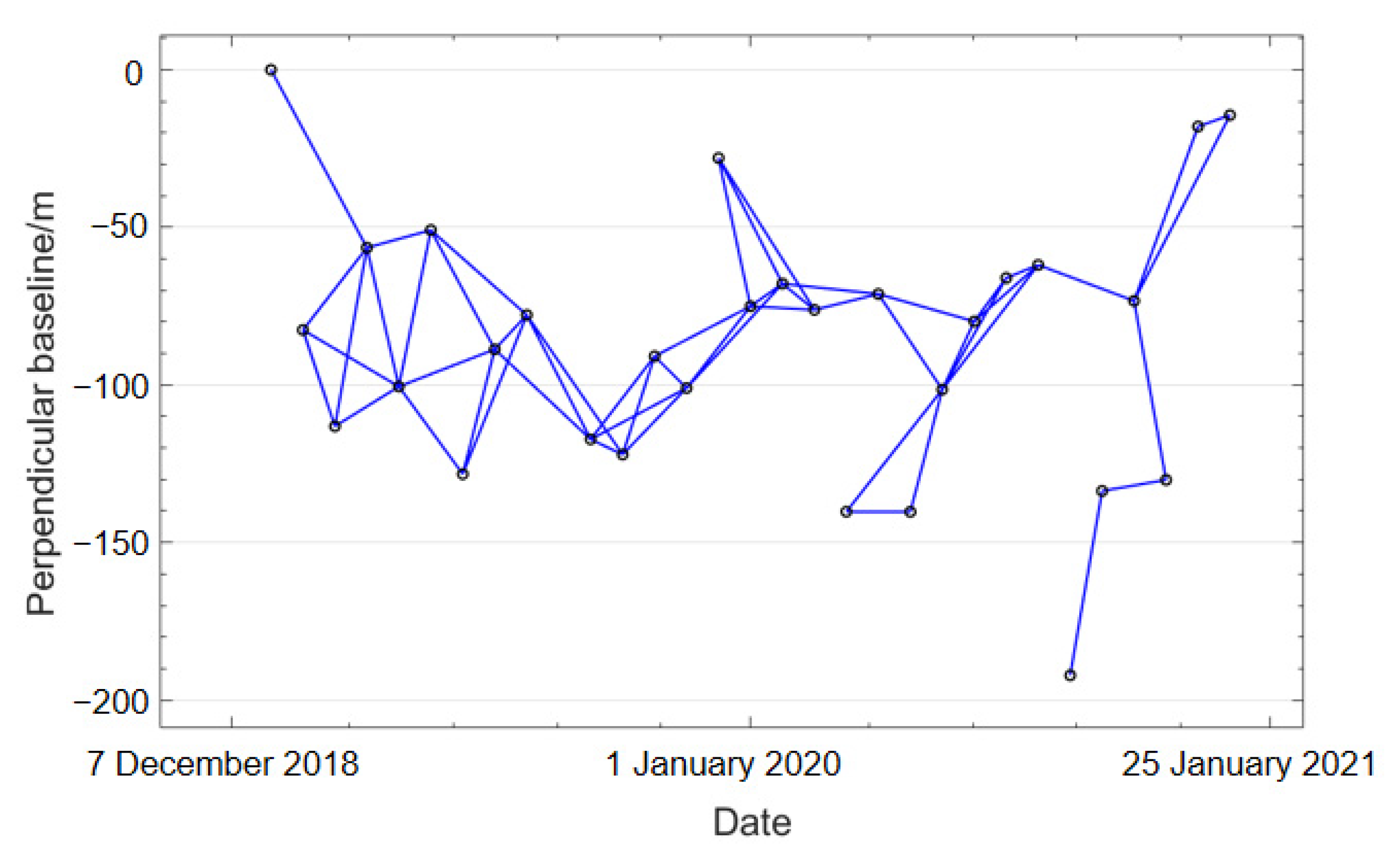
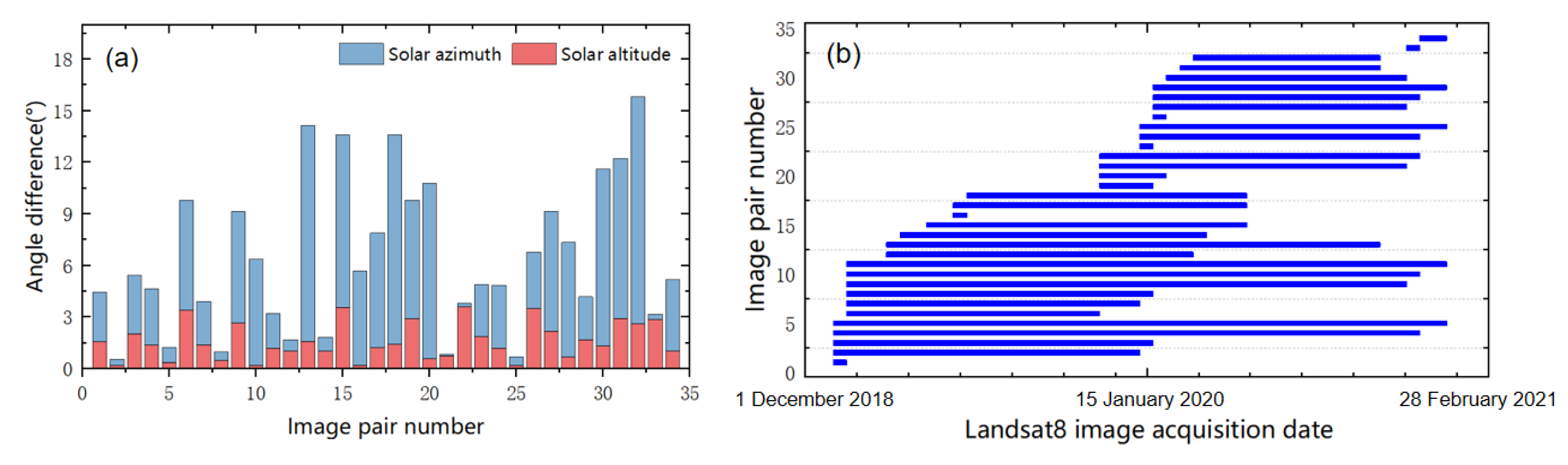
The experimental area was located at Shishapangma Peak, a peak in the middle of the Himalayas in Nyalam County, Tibet Autonomous Region, China. The geospatial locations are shown in Figure 1a. The central Himalayas is covered with many glaciers and is the source of many rivers, such as the Ganga River, Jumna River and Bilangna River. In recent years, glaciers have melted, and glaciers in the central Himalayas are more likely to collapses, glacial lakes, and floods than in other areas. The Shishapangma region is one of the centers of modern glaciation and is crisscrossed by many mountain glaciers [18]. As a result of climate change, glaciers are melting at faster rates, and the number of glacial lakes has increased, exacerbating the occurrence of natural disasters, such as glacial lake outbursts and debris flows [19]. From 1988 to 2015, the glacier area in the Jilong River Basin of Tibet decreased by 16.45% [20]. Similarly, the area of glacial lakes in the Boqu Basin, Tibet, increased by 110% from 1964 to 2017, and eight glacial lakes were considered potentially dangerous [21]. The research object of this study is the large glacier of Shishapangma Peak, as shown in Figure 1b. The upper reaches of the glacier have three tributaries and converge in the middle reaches, which is a typical experimental area for the analysis of glacier three-dimensional motion characteristics.

2.2. Study Data

Considering that image pairs with long time intervals are more beneficial for displacement estimation, 31-scene Sentinel-1 ascending orbit images with 24 d intervals from the official website of the European Space Agency were selected. The study period chosen was January 2019 to December 2020. Detailed parameter information is presented in

Table 1. Sentinel-1 image parameters.

Orbit Direction	Ascending
Track No.	85
Incidence angle at scene center (°)	33.9°
Azimuth angle (°)	−10.1°
Imaging mode	Interferometric Wide swath
Polarization mode	VV
Number of scenes	31
Acquisition period (yyyymmdd)	6 January 2019–26 December 2020

. A total of 19 Landsat 8 operational land imager (OLI) optical images from the USGS were used, and the image coverage is shown in Figure 1a. The time range of the Landsat 8 images was from January 2019 to January 2021, and the parameter information is shown in

Table 2. Landsat 8 image parameters.

Image Bands	Panchromatic Band
Spatial resolution/m	15
Data Product level	Level-1T
Central wavelength/μm	0.59
Revisit cycle/d	16
Number of scenes	19
Acquisition period (yyyymmdd)	3 January 2019–8 January 2021

. These Landsat 8 images were ortho-corrected based on an external DEM [22].

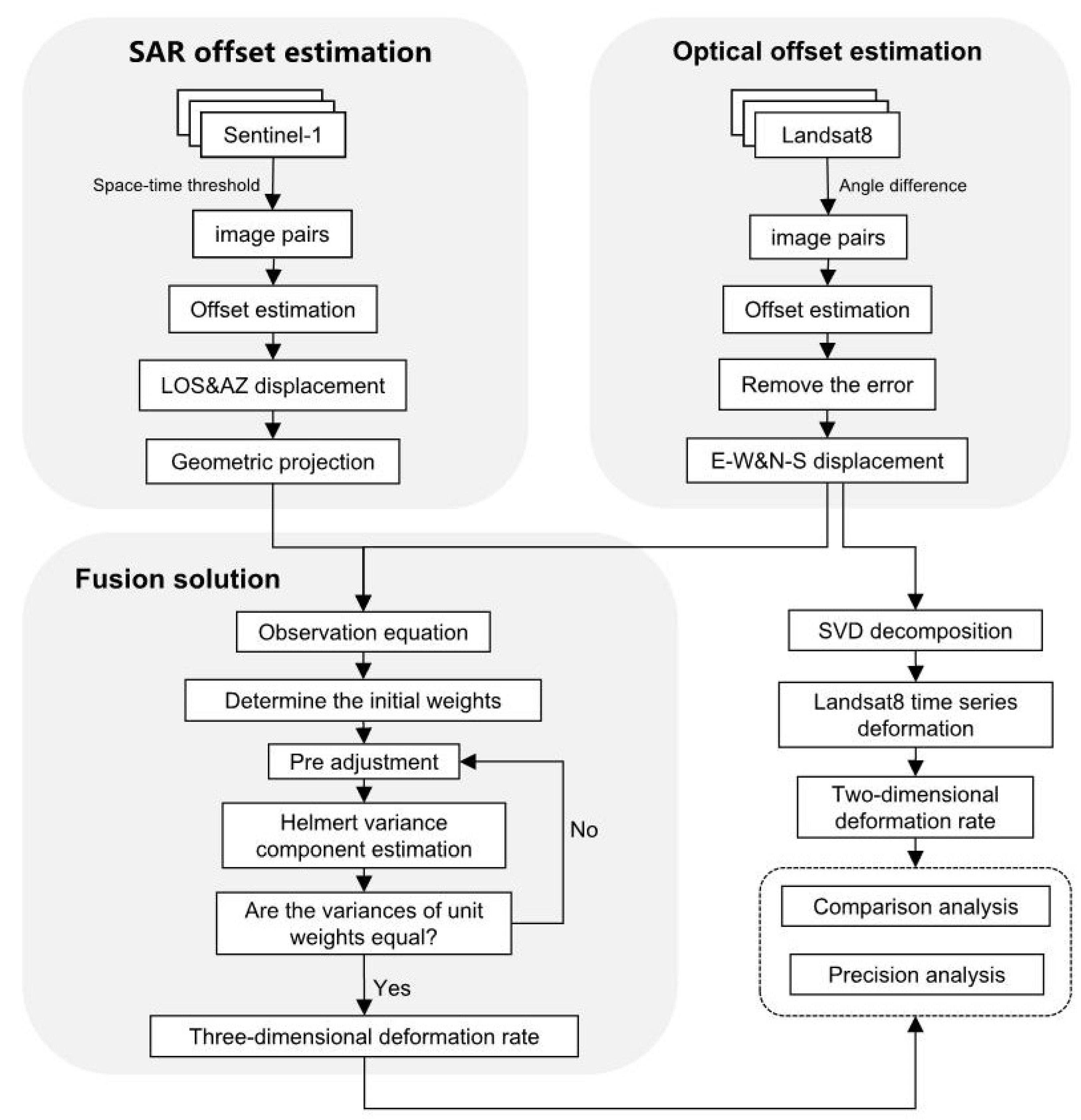
3. Methods and Data Processing

In this paper, the method of pixel offset tracking technology and variance component estimation is mainly used to reverse the 3D flow velocity of glaciers. Based on offset tracking technology, Sentinel-1 images can be used to obtain the displacement of the target in the range and azimuth directions of SAR images, and Landsat 8 images can be used to obtain the displacement of the target in the east–west and south–north directions. The optimal estimation of the three-dimensional velocity of the glacier was obtained by integrating the displacement of the above four directions with the variance component estimation. Data processing is divided into three main steps: SAR offset estimation, optical offset estimation, and fusion solution (Figure 2).

The specific steps to estimate the variance components are as follows: First, the SAR image was processed using pixel offset tracking technology to obtain the displacement results of the target pixels in the range and azimuth directions. The displacement results were transformed by projection and resampling, and the displacements in the east–west, north–south, and vertical directions were decomposed. At the same time, pixel offset tracking technology was also used to process Landsat 8 images to obtain the displacement results of target pixels in the east–west and south–north directions. Then, according to the different error sources of the measurement results, the range and azimuth displacements obtained by SAR offset tracking, and the east–west and south–north displacements obtained by optical offset tracking were composed of four observation equations. Based on the variance component estimation, the stochastic model posterior estimation of the SAR offset and optical offset displacement results was performed, and the optimal 3D deformation rate estimation of the glacier was obtained.

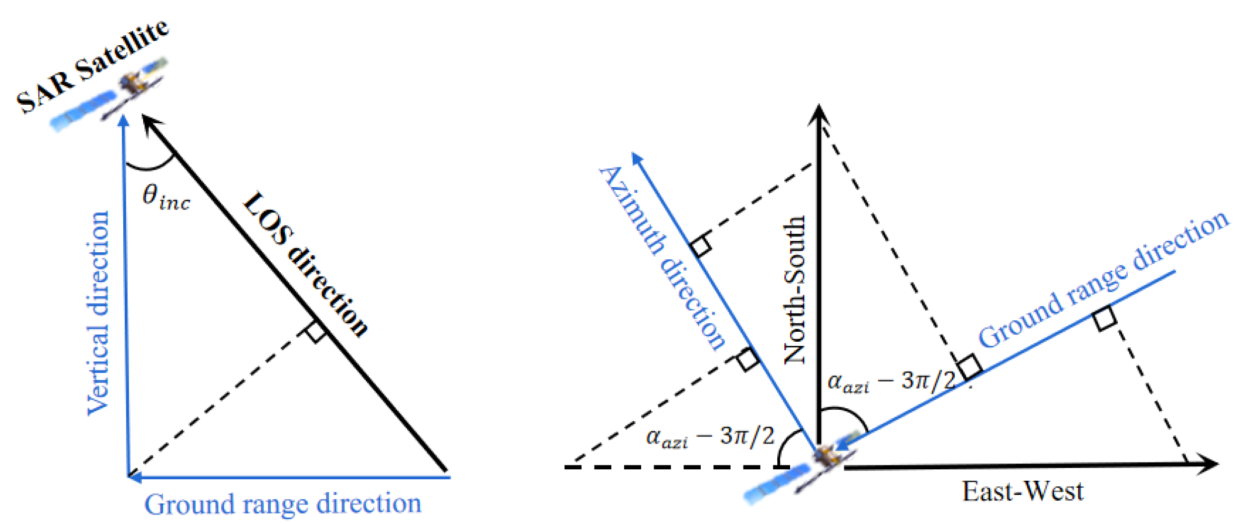
3.1. SAR Offset Estimation

The offset tracking technology based on SAR images uses a normalized cross-correlation algorithm to obtain the offset in the range and azimuth directions. Since the calculation results will be affected by the incoherent noise of SAR images, the small baseline set pixel tracking algorithm [23] is adopted in this paper. First, the optimal baseline combination was obtained by setting spatial and temporal threshold values (Figure 3). Then, the offset was estimated using the intensity-tracking algorithm, which requires less coherence. To obtain high-precision offset results, the search window size was set to 128 × 128 pixels (range × azimuth), the search step was 5 × 1 pixels (range × azimuth), and the correlation coefficient threshold was 0.2. These settings were designed to balance the offset signal and noise generated by the estimation process.

3.2. Optical Offset Estimation

The pixel offset tracking algorithm based on optical images uses the sub-pixel correlation matching algorithm to obtain the offset results in the east–west and south–north directions. Because the Cosi-corr software can usually obtain good accuracy and reliability [24], it was used to estimate the offset between the optical images in our study. The offset tracking results of the optical system are affected by the uncorrelated noise and the solar angle [12]. The larger the angle difference between the two images, the larger the error is. Therefore, we calculated the difference between the solar altitude angle and solar azimuth angle between each image pair before the offset tracking processing. Figure 4a shows 34 optical image pairs with a small difference between solar altitude angle and solar azimuth angle (the solar altitude angle difference is less than 3.58; the solar azimuth angle difference is less than 15.82). Figure 4b shows the time baseline of 34 image pairs.

In processing with the Cosi-corr software, we adopted a two-level window search strategy to obtain more accurate results. First, we set the window size to 64 × 64 for the initial search to reduce the effect of outliers on the image matching accuracy and then set the search window size to 32 × 32 to obtain more deformation details. Then, we set the search step to four pixels and the number of iterations to two. We masked the uncorrelated noise according to the amplitude of the log-cross-correlated spectrum using a mask threshold of 0.9. The offset of the image pair was estimated based on the frequency domain cross-correlation algorithm, and the displacement in the east–west and north–south directions and signal-to-noise ratio (SNR) were obtained. The errors caused by uncorrelated noise in the north–south and east–west results were further removed by selecting pixels with an SNR greater than 0.9. The orbit error in the offset result was removed using the polynomial surface-fitting model. Owing to the marked and uniformly distributed linear signals forming strip errors along the orbit direction of the push-broom imaging satellite, the strip errors were removed from the offset results by means of mean subtraction [25]. Simultaneously, the final offset results were processed using non-mean filtering to smooth the influence of local noise. The optical image time-series offset results were solved using the singular value decomposition (SVD) method. The results of the time-series displacement were obtained by integrating the deformation rate with time (Figure 2).

3.3. Fusion Solution Based on Variance Component Estimation

As a joint adjustment method for multi-category data, Helmert variance component estimation can usually obtain the optimal estimate of observations. First, we classified the observed values according to their different sources and determined the initial weight and pre-adjustment of each value. Then, the posterior unit weight variance of various values was calculated according to certain principles. The iterative operation of the observation quantity was performed until the errors in their unit weights were equal or the ratio of the variances of all types of unit weights is equal to 1. Some scholars have studied the fusion of InSAR and GPS observations using this method [26]. In this study, the posterior estimate of the stochastic model was used to estimate the SAR and optical displacements using variance component estimation. The basic principles and processes are as follows.

To solve the problem of unequal pixel sizes of Sentinel-1 and Landsat 8 images, we carried out coordinate system conversion and pixel resampling. First, the Sentinel-1 images coordinate system was converted to a coordinate system consistent with Landsat 8’s. The Sentinel-1 images are then resampled to a resolution consistent with Landsat’s 8-pixel size.

We assumed that N SAR images form m interference pairs. For coherence point i in the rth ($1\le r\le$ m) image pair, assuming uniform deformation occurs, then

$$Lo{s}^{ri}=[t_r·C_e^{ri} t_r·C_n^{ri} t_r·C_u^{ri} ]·{\left[v_e^i{v}_n^i{v}_u^i\right]}^T$$

(1)

$$A{z}^{ri}=[t_r·D_e^{ri} t_r·D_n^{ri} t_r·D_u^{ri} ]·{\left[v_e^i{v}_n^i{v}_u^i\right]}^T$$

(2)

where $Lo{s}^{ri}$ and $A{z}^{ri}$ are the deformation in the line of sight (LOS) and the azimuth of coherence point i in the rth interference pair, respectively. $v_e^i,v_n^i,\mathrm{and}{v}_u^i$ are the deformation rates of point i in the east–west, north–south, and vertical directions, respectively. $t_r$ is the time interval of the rth interference pair. $C_e^i, C_{n }^i,$ and $C_u^i$ are the projections of the LOS direction on coherence point i in the east–west, north–south, and vertical directions, respectively. $D_e^{ri},D_n^{ri}$, and $D_u^{ri}$ are the projections of the azimuth direction on coherence point i in the east–west, north–south, and vertical directions, respectively. The values were calculated according to the geometric relationship of the projection (Figure 5) using the following equations:

$$\left\{\begin{array}{c}{C}_e^i=-\sin {\theta }_{inc}^i\sin \left({\alpha }_{azi}^i-3\pi /2\right)\\ C_n^i=-\sin {\theta }_{inc}^i\cos \left({\alpha }_{azi}^i-3\pi /2\right)\\ C_u^i=\cos {\theta }_{inc}^i\\ D_e^i=-\cos \left({\alpha }_{azi}^i-3\pi /2\right)\\ D_n^i=-\sin \left({\alpha }_{azi}^i-3\pi /2\right)\\ D_u^i=0\end{array}\right.$$

(3)

where ${\theta }_{inc }^i$ and ${\alpha }_{azi}^i$ are the incidence and azimuth angles on coherence point i, respectively.

If f image pairs are formed using optical images for the coherence point i of the kth image pair ($1\le k\le f$), then

$${\left[Q_e^{ki}{Q}_n^{ki}\right]}^T=t_k·{\left[v_e^i{v}_n^i\right]}^T$$

(4)

where $Q_e^{ki}$ and $Q_n^{ki}$ are the deformations of coherence point i in the east–west and north–south directions, respectively.

Three-dimensional surface deformation was solved based on the least square model fusion of SAR interferometric pairs observation and optical image pairs observation:

$$L=BX+V$$

(5)

where $\underset{3\times 1}{X}$ = ${\left[v_e^i{v}_n^i{v}_u^i\right]}^T$ is the 3D deformation rate of the solution; $\underset{2(\mathrm{m}+f)\times 1}{L}$ = [$Lo{s}^{1i}\cdots$ $Lo{s}^{mi}$ $A{z}^{1i}$ $\cdots$ $A{z}^{mi}$ $Q_e^{1i}$ $\cdots$ $Q_e^{fi}$ $Q_n^{1i}$ $\cdots$ $Q_n^{fi}$]^T is the SAR offset measurements and optical offset observations; V is the corresponding observation residuals; and B is a matrix composed of the observed values in the three directions:

$$\underset{2(\mathrm{m}+f)\times 3}{B}= {\left[\begin{array}{ccc}{t}_1·C_e^{1i} \cdots t_m·C_e^{mi}& t_1·D_e^{1i} \cdots t_m·D_e^{mi}& t_1 \cdots t_f\\ t_1·C_n^{1i} \cdots t_m·C_n^{mi}& t_1·D_n^{1i} \cdots t_m·D_n^{mi}& 0 \cdots 0\\ t_1·C_u^{1i} \cdots t_m·C_u^{mi}& t_1·D_u^{1i} \cdots t_m·D_u^{mi}& 0 \cdots 0\end{array} \begin{array}{c}0 \cdots 0\\ t_1 \cdots t_f\\ 0 \cdots 0\end{array}\right]}^T$$

(6)

Assuming that the variance of the observed value is known, the optimal valuation of the 3D deformation rate can be calculated by the least-squares adjustment:

$$\widehat{X}=(B^{T}PB{)}^{-1}{B}^{T}PL$$

(7)

where $P$ is the weight matrix composed of the variance of each observation and

$$\underset{2(\mathrm{m}+f)\times 2(m+f)}{{\displaystyle P}}=\mathrm{diag}\left(1/{\mathsf{\sigma }}_{{\mathrm{Los}}^{1\mathrm{i}}}^2\cdots 1/{\mathsf{\sigma }}_{{\mathrm{Los}}^{\mathrm{mi}}}^{2}1/{\mathsf{\sigma }}_{{\mathrm{Az}}^{1\mathrm{i}}}^2\cdots 1/{\mathsf{\sigma }}_{{\mathrm{Az}}^{\mathrm{mi}}}^{2}1/{\mathsf{\sigma }}_{{\mathrm{Q}}_{\mathrm{e}}^{1\mathrm{i}}}^2\cdots 1/{\mathsf{\sigma }}_{{\mathrm{Q}}_{\mathrm{e}}^{\mathrm{fi}}}^{2}1/{\mathsf{\sigma }}_{{\mathrm{Q}}_{\mathrm{n}}^{1\mathrm{i}}}^2\cdots 1/{\mathsf{\sigma }}_{{\mathrm{Q}}_{\mathrm{n}}^{\mathrm{fi}}}^2\right)$$

(8)

To obtain the optimal estimation of the 3D deformation rate, in addition to the functional model, a stochastic model of the observations is required, and the weights can be accurately determined in the adjustment model. Usually, it is difficult to obtain the variance of the observed values accurately. Therefore, a posteriori estimation can be conducted based on the variance component estimation. As mentioned above, the observation error of SAR offsets is affected by incoherence, oversampling, and matching windows, whereas the observation error of optical offsets is affected by various noises, matching windows, and step sizes. Therefore, according to the different observation errors, the range and azimuth directions of SAR observations and the east–west and south–north directions of the optical image observations constitute four groups of observations. Assuming that each set of observations is $L_i$ and the weight is $P_i$ (i = 1, 2, 3, 4), the first valuation is obtained based on the least-squares method:

$$\left\{\begin{array}{c}\widehat{X}=N^{-1}W\\ V_1=B_1\widehat{X}-L_1\\ V_2=B_2\widehat{X}-L_2\\ V_3=B_3\widehat{X}-L_3\\ V_4=B_4\widehat{X}-L_4\end{array}\right.$$

(9)

where $L={\left[\begin{array}{cccc}{L}_1& L_2& L_3& L_4\end{array}\right]}^T$, $B={\left[\begin{array}{cccc}{B}_1& B_2& B_3& B_4\end{array}\right]}^T$, $P=diag{\left[\begin{array}{cccc}{P}_1& P_2& P_3& P_4\end{array}\right]}^T$, $N=B^{T}PB={\displaystyle \sum _{\mathrm{i}=1}^4{B}_i^T}{P}_i{B}_i={\displaystyle \sum _{\mathrm{i}=1}^4{N}_i^{}}$, $W=B^{T}PL={\displaystyle \sum _{\mathrm{i}=1}^4{B}_i^T}{P}_i{L}_i$.

$$\widehat{\theta }=S^{-1}{W}_{\theta }$$

(10)

where $\widehat{\theta }={\left[\begin{array}{cccc}{\widehat{\sigma }}_{0_1}^2& {\widehat{\sigma }}_{0_2}^2& {\widehat{\sigma }}_{0_3}^2& {\widehat{\sigma }}_{0_4}^2\end{array}\right]}^T$ is the error in the unit weight of the four observed values, $W_{\theta }={\left[\begin{array}{cccc}{V}_1^T{P}_1{V}_1& V_2^T{P}_2{V}_2& V_3^T{P}_3{V}_3& V_4^T{P}_4{V}_4\end{array}\right]}^T$, and $S=\left[\begin{array}{cccc}\mathrm{m}-2tr(N^{-1}{N}_1)+tr{(N^{-1}{N}_1)}^2& tr(N^{-1}{N}_1{N}^{-1}{N}_2)& tr(N^{-1}{N}_1{N}^{-1}{N}_3)& tr(N^{-1}{N}_1{N}^{-1}{N}_4)\\ tr(N^{-1}{N}_1{N}^{-1}{N}_2)& \mathrm{m}-2tr(N^{-1}{N}_2)+tr{(N^{-1}{N}_2)}^2& tr(N^{-1}{N}_2{N}^{-1}{N}_3)& tr(N^{-1}{N}_2{N}^{-1}{N}_4)\\ tr(N^{-1}{N}_1{N}^{-1}{N}_3)& tr(N^{-1}{N}_2{N}^{-1}{N}_3)& \mathrm{f}-2tr(N^{-1}{N}_3)+tr{(N^{-1}{N}_3)}^2& tr(N^{-1}{N}_3{N}^{-1}{N}_4)\\ tr(N^{-1}{N}_1{N}^{-1}{N}_4)& tr(N^{-1}{N}_2{N}^{-1}{N}_4)& tr(N^{-1}{N}_3{N}^{-1}{N}_4)& \mathrm{f}-2tr(N^{-1}{N}_4)+tr{(N^{-1}{N}_4)}^2\end{array}\right]$ Finally, the new weight estimate is calculated.

$${\widehat{P}}_1=P_1,{\widehat{P}}_2=\frac{{\sigma }_{0_1}^2}{{\sigma }_{0_2}^2{P}_2^{-1}},{\widehat{P}}_3=\frac{{\sigma }_{0_1}^2}{{\sigma }_{0_3}^2{P}_3^{-1}},{\widehat{P}}_4=\frac{{\sigma }_{0_1}^2}{{\sigma }_{0_4}^2{P}_4^{-1}}$$

(11)

Substituting the obtained new weight array estimate into Equation (9) to calculate the least squares estimate and iterating through Equations (9) to (11) until:

$${\widehat{\sigma }}_{0_1}^2\approx {\widehat{\sigma }}_{0_2}^2\approx {\widehat{\sigma }}_{0_3}^2\approx {\widehat{\sigma }}_{0_4}^2$$

(12)

When the cycle iteration ends, ${\widehat{P}}_1$, ${\widehat{P}}_2$, ${\widehat{P}}_3$, ${\widehat{P}}_4$ is the weight matrix obtained by using the variance component estimation, which can be substituted into Equation (9) to obtain the optimal 3D deformation rate.

4. Results and Analysis

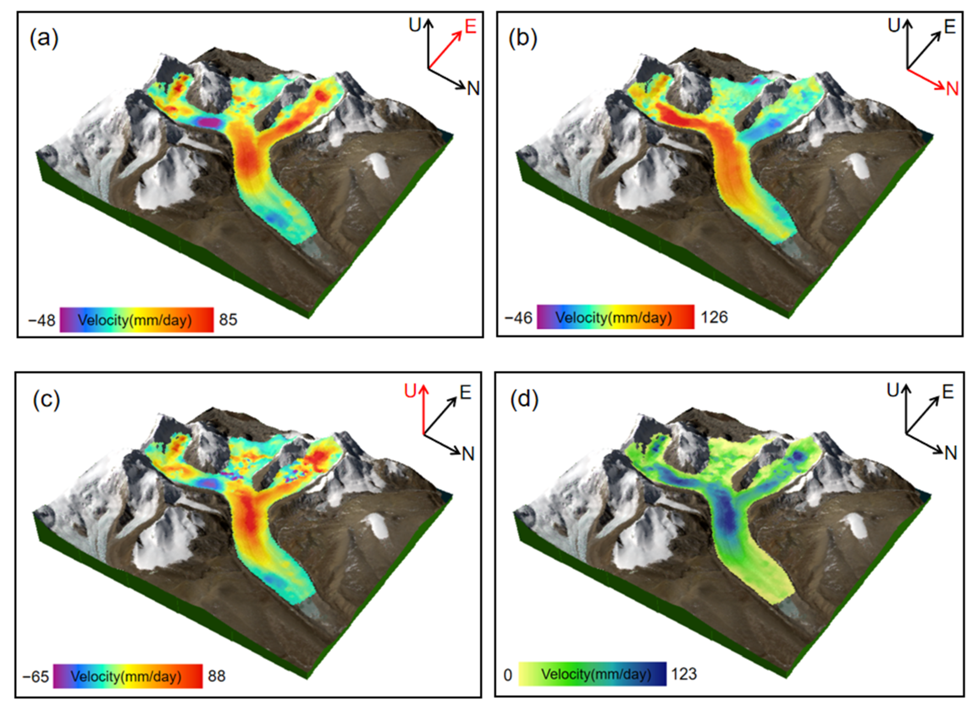
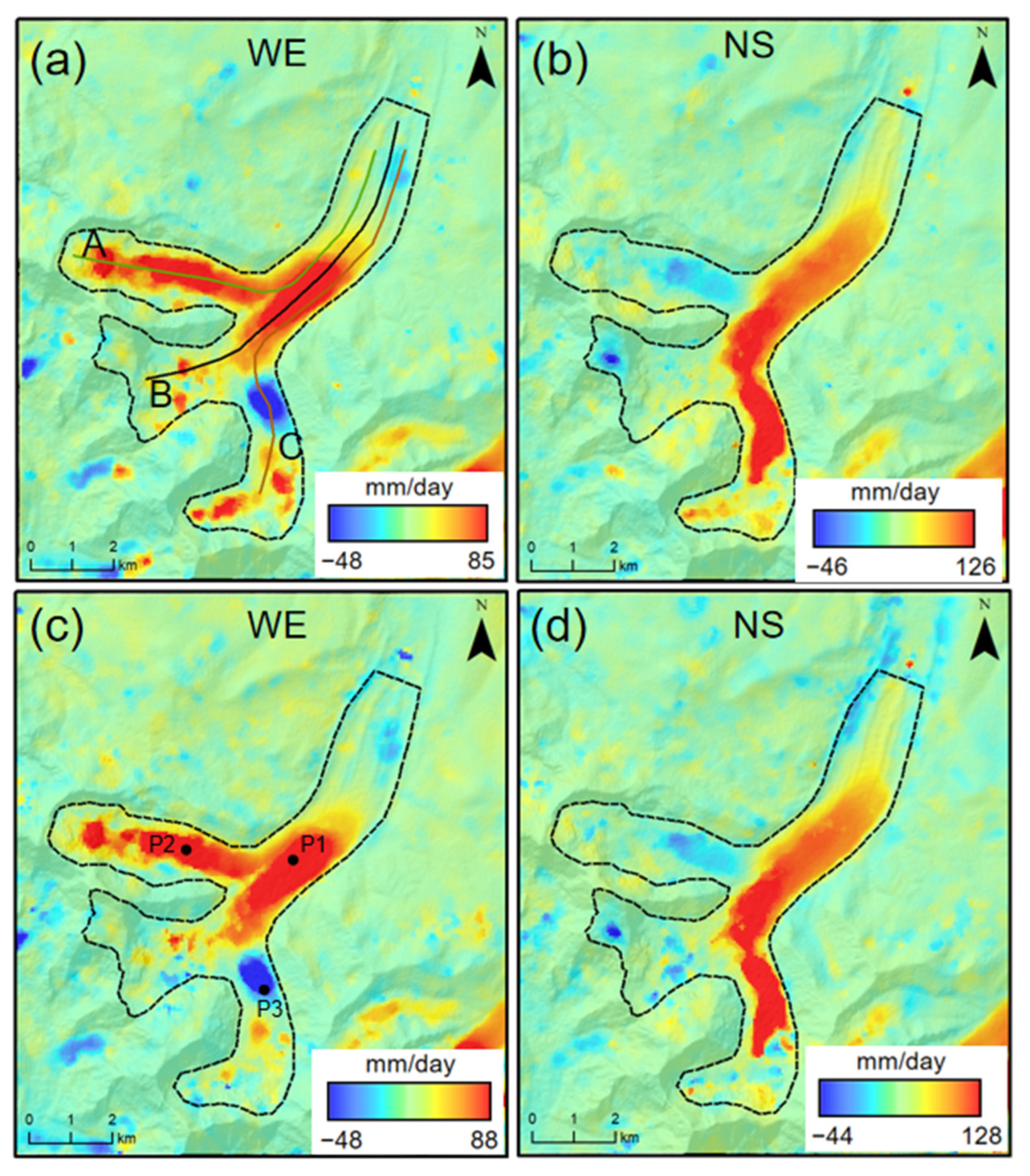
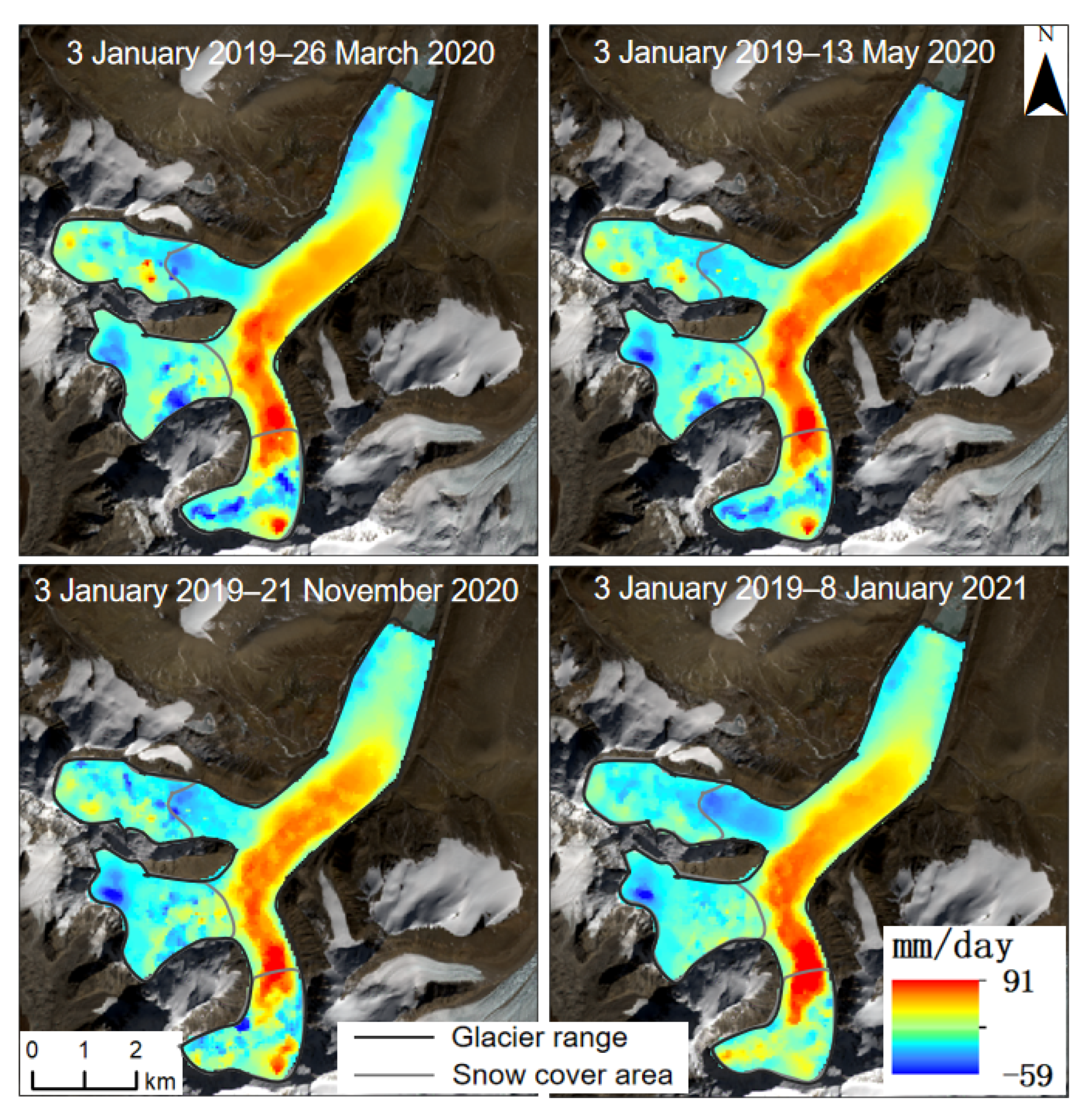
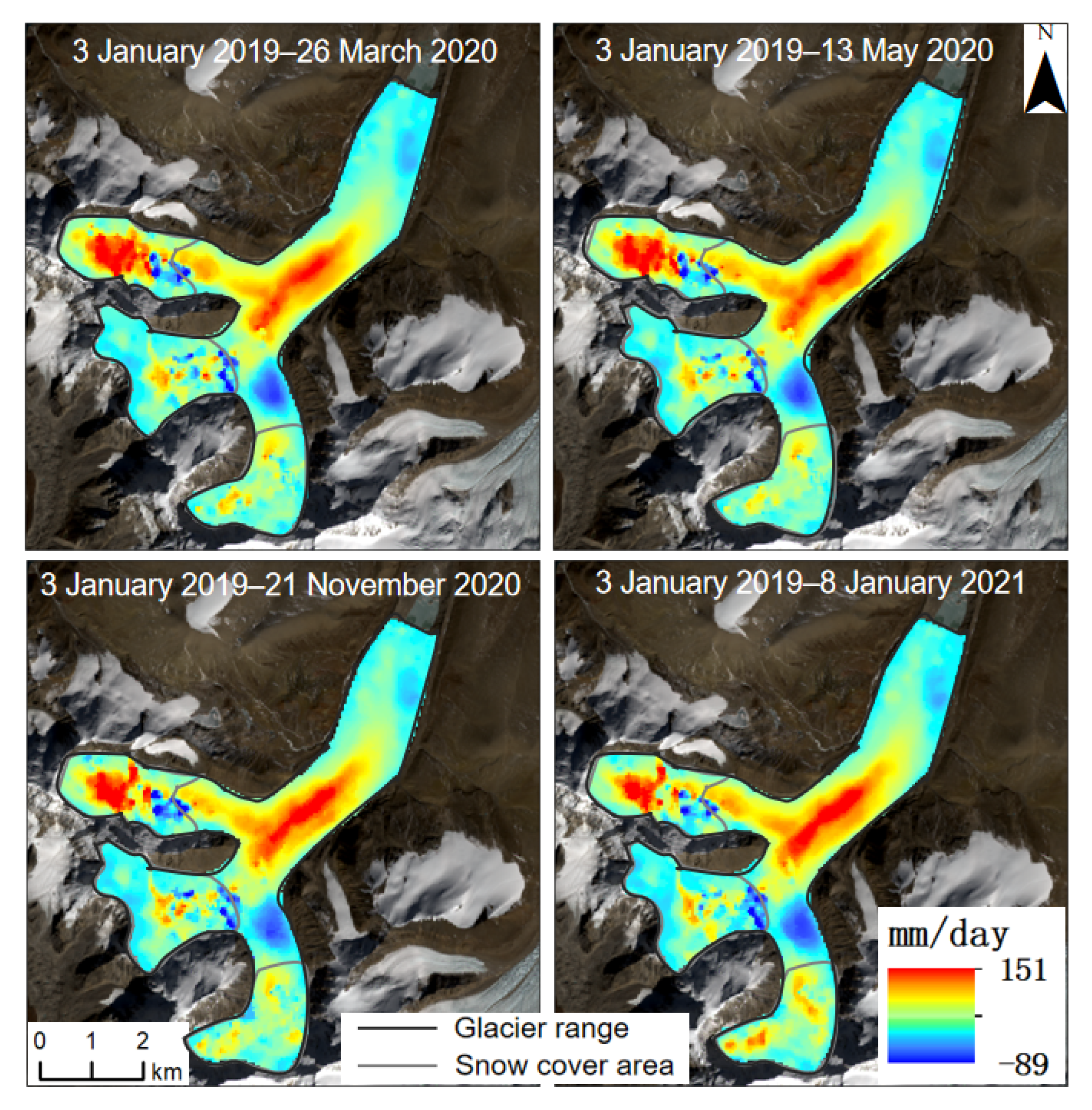
4.1. Glacier Displacement Results with SAR and Optical Offset

By fusing the offset results of Sentinel-1 SAR and Landsat 8 images, the glacier 3D deformation rate was obtained, as shown in Figure 6. The results show that the maximum deformation rate of the glacier was 85 mm/day in the west–east direction (Figure 6a), 126 mm/day in the north–south direction (Figure 6b), and 88 mm/day in the vertical direction (Figure 6c). This indicates that the movement speed of the upper reaches of the glacier was faster, that of the middle reaches was slower, and that of the downstream gradually decreased. Because of the large topographic fluctuation change and the ablation area in the upstream part of the glacier, the flow velocities of the three branches in the upstream changed significantly, and there was local information discontinuity caused by the disappearance of feature points. Next, the west–east, north–south, and vertical flow velocities after the joint calculation were synthesized, as shown in Figure 6d. Overall, glacier movement was characterized by north–east flow from the south–west, which is consistent with the actual flow direction of the glaciers. The areas with a large surface flow rate include the ablation area of the upstream glaciers, the area with a large slope, and the confluence of the three upstream glacier tributaries.

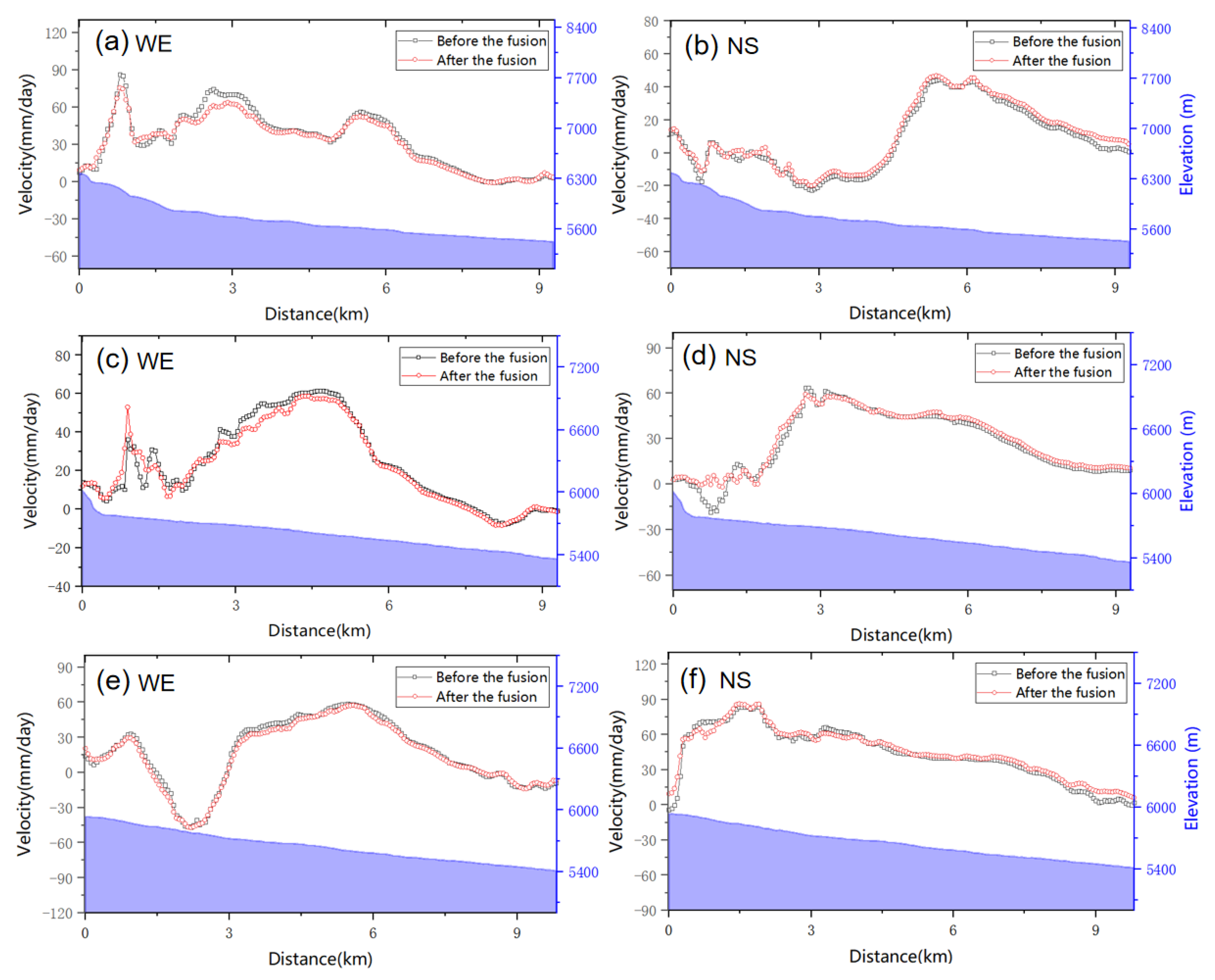
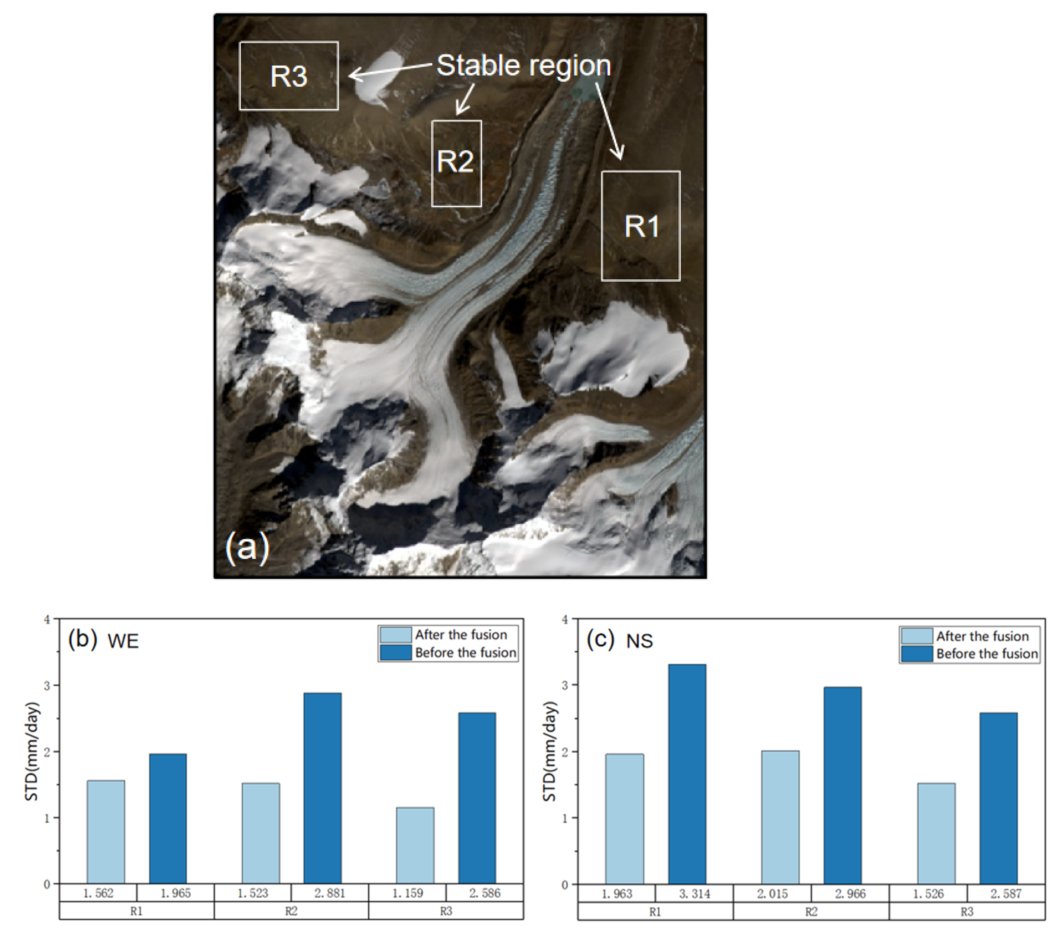
4.2. Comparative Analysis

To test the reliability of the glacier displacement and its motion characteristics calculated by the combined model, the fusion results in the north–south (Figure 7a) and west–east (Figure 7b) directions were compared with the glacial velocity calculated using the optical offset timing (Figure 7c,d) in the same period. The optical offset results were chosen for comparison for two reasons. First, the results of the optical time-series offset were consistent with the joint solution in the north–south and west–east directions. Secondly, the pixel size of the optical time-series offset was consistent with that of the joint solution. As shown in Figure 7, the fusion results were consistent with the optical image offset calculation results. The area with a large movement rate was the upper upstream glacier ablation area and the middle tributary collection area. Because optical image offset technology could not be used to calculate the vertical displacement, the vertical displacement results originated entirely from the decomposition of the SAR offset in the range and azimuth directions. Furthermore, because no other monitoring data could be used, we could not compare the vertical displacement of the glacier with other measures.

Figure 8 shows the difference in values of the two methods in the west–east and north–south directions. It can be seen that the regions with great differences were the ablation regions of the three tributaries upstream of the glacier (K1, K2, and K3) (Figure 8). The largest difference was observed in the K1 area. This is because some low-quality points caused by the large variation in the scattering characteristics of glaciers in the optical image were removed during processing. With fusion processing, the flow velocity information in the low-quality areas of the glaciers could be obtained.

To further compare the joint solution results with the optical results, we extracted the north–south and west–east flow velocity profiles based on the mainstream direction of the glacier (A, B, and C in Figure 7a). The profile results are shown in Figure 9. In the west–east direction, the main difference between the results before and after the joint solution existed upstream of the glacier. Especially in profiles A and B (Figure 9a,c), the maximum velocity difference reached 13.13 and 16.79 mm/day, respectively. In the north–south direction, the main difference between the results before and after the joint solution was found upstream of the glacier (Figure 9b,d,f). The maximum difference reached 6.36, 18.26 and 12.89 mm/day, respectively. At the same time, differences were also observed downstream of profiles A and C (Figure 9b,f). Because the glacier surface characteristics change the most in the upstream and downstream regions, the spectral reflection information of the optical image was easily affected by errors in these areas, resulting in the significant fluctuation of the solution in both the upstream and downstream regions. In contrast, the joint solution model selected points with smaller errors in both data results to calculate the three-dimensional displacement of the glacier. Therefore, the joint solution results were more reliable.

5. Discussion

5.1. Precision Analysis

As we failed to collect the measured data of glacier displacement in the study area, the standard deviation of the non-glacial stable area was used for accuracy analysis, and the optical time-series offset in the same direction was compared with the results of the joint solution. To this end, we selected three stable areas of non-glacier bare surfaces without snow cover, namely R1, R2, and R3 in Figure 10a, and counted the standard deviation of the fusion and optical results, as shown in Figure 10b,c. In the west–east direction, the standard deviations of the Landsat 8 results were 1.965, 2.881, and 2.586 mm/d, while those of the fusion results were 1.562, 1.523, and 1.159 mm/d, respectively. The west–east joint results improved by 21%, 47%, and 55% over that of the optical. In the south–north direction, the standard deviation of the Landsat 8 results were 3.314, 2.966, and 2.587 mm/d, while those of the fusion results were 1.963, 2.015, and 1.526 mm/d, respectively. The north–south joint results improved by 41%, 32%, and 41% over the optical results. In general, the uncertainty in the glacier displacement monitoring results of the fusion solution was less than that of the optical results. This indicates that the joint solution method can effectively improve the accuracy and reliability of the results.

To verify the accuracy of the fused glacier displacement results, we acquired glacier cataloging dat afrom the Shishapangma peak region in 2018 [27]. The end of the glacier in the experimental area was covered with a moraine glacier (Figure 11a). Because the flow velocity of a moraine glacier is low, it was difficult to accurately obtain the surface flow velocity using an offset tracking technique. Thus, the boundary information of the glacier cataloging data was used to evaluate the accuracy of the monitoring results. The velocity in the region of the moraine glacier after fusion (Figure 11b) was more accurate than that without fusion (Figure 11c). The fusion result was more consistent with the vector boundary of the glacier-cataloging data. Simultaneously, the fused glacier velocity could be used as a velocity factor to extracting the glacier more accurately.

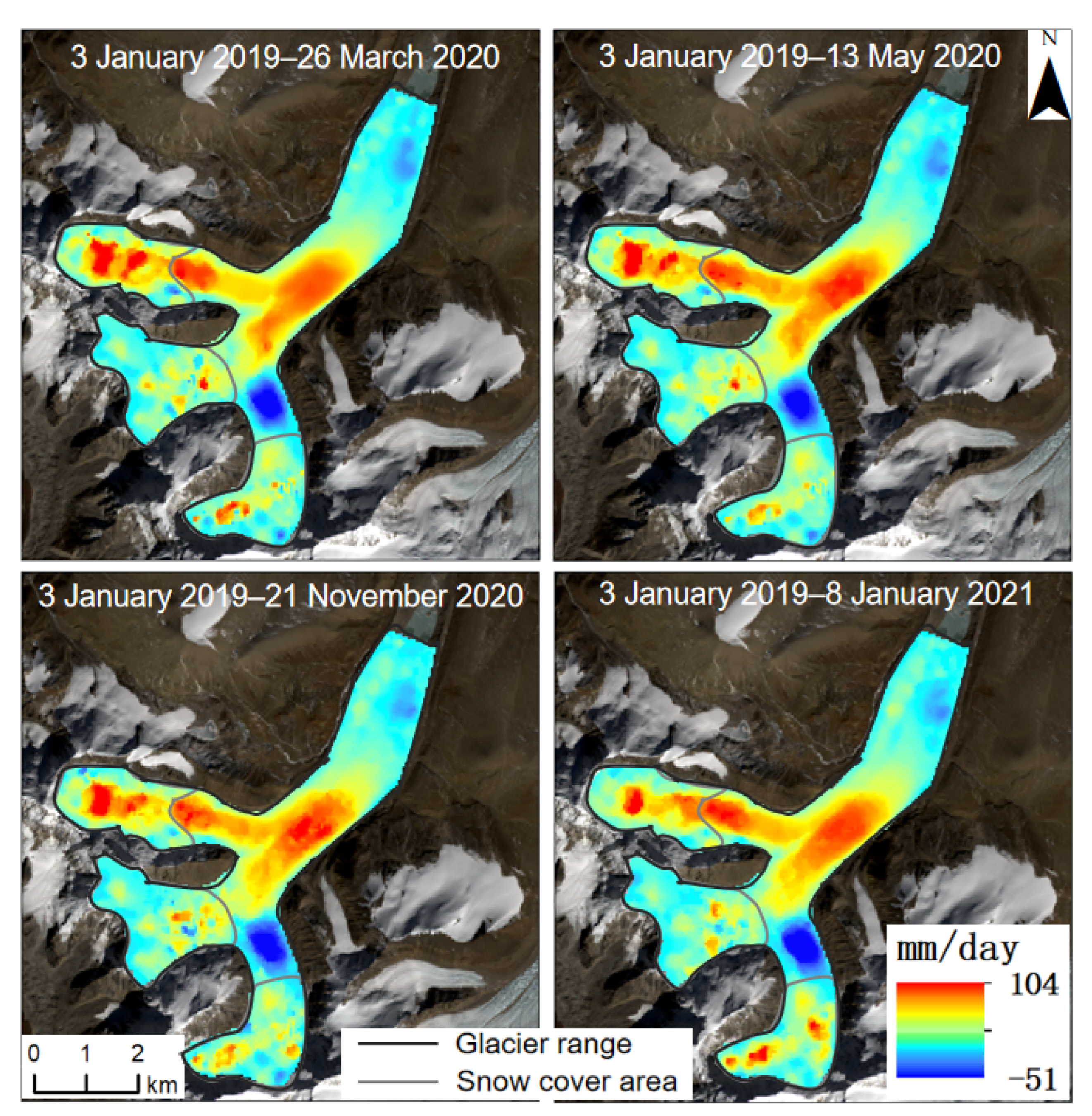
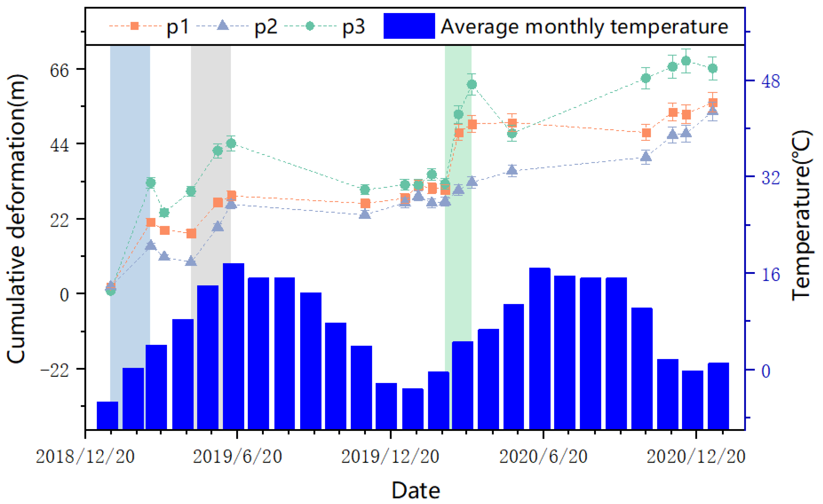
5.2. Glacier Time-Series Displacement

Based on variance component estimation, the displacement results of the glacier surface time series could be obtained with high accuracy. However, more SAR and optical image pairs were required to achieve higher accuracy. Because optical images are easily affected by meteorological conditions, the SAR image pairs involved in our experiment were sufficient, and the number of optical image pairs was small. Therefore, the period in which both optical and SAR image pair numbers were greater than 12 (

Table 3. Number of SAR and optical image pairs involved in the study of different periods.

Time Range	3 January 2019–26 March 2020	3 January 2019–13 May 2020	3 January 2019–21 November 2020	3 January 2019–8 January 2021
Number of SAR image pairs	34	37	51	54
Number of optical image pairs	13	16	20	34

) was selected to calculate the west–east (Figure 12), north–south (Figure 13), and vertical (Figure 14) time-series velocity of the glacier. The time-series results of the four periods were obtained, as shown in Figure 12 and Figure 14. The confluence area of the glaciers showed strong three-dimensional movement characteristics.

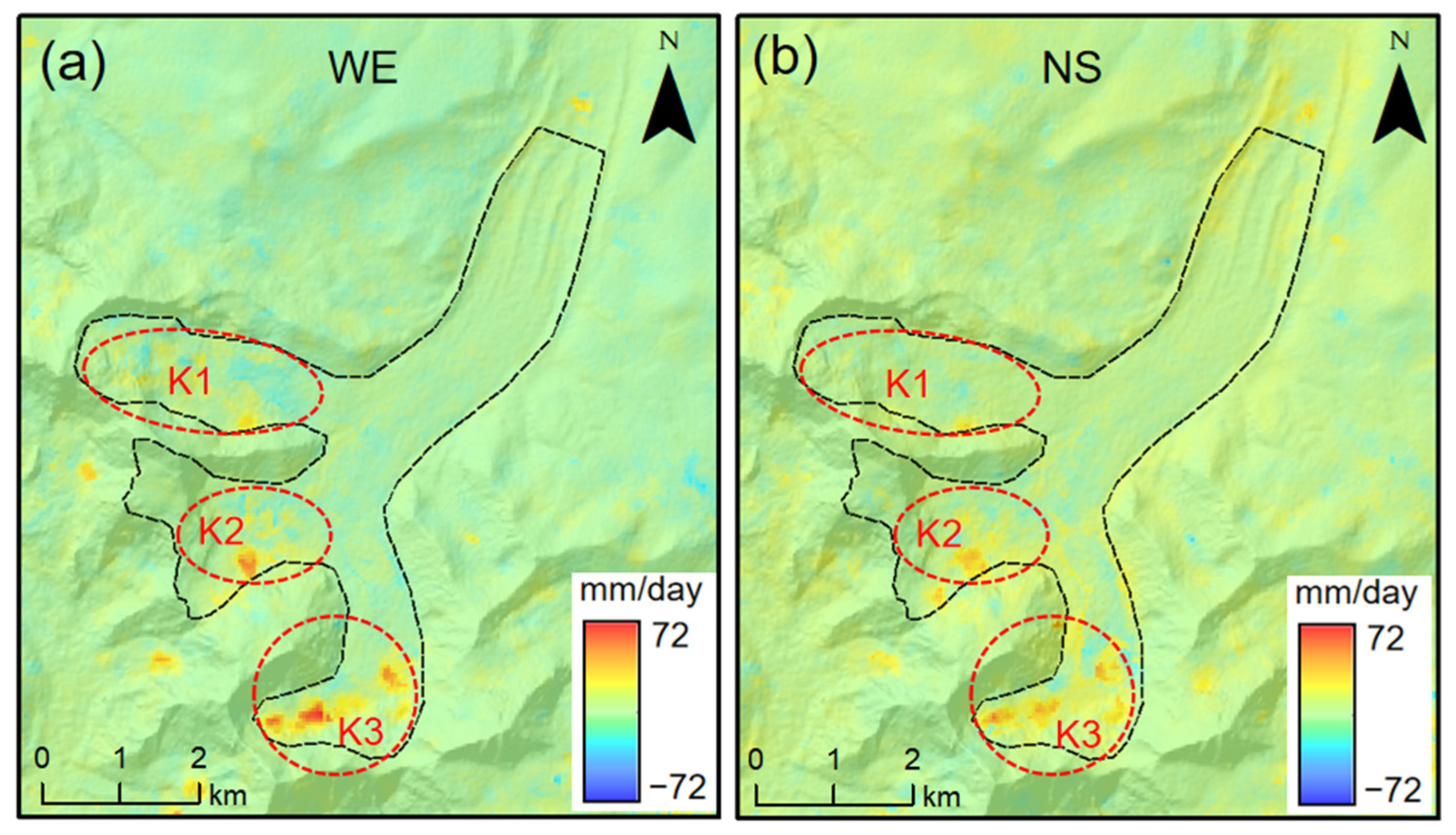
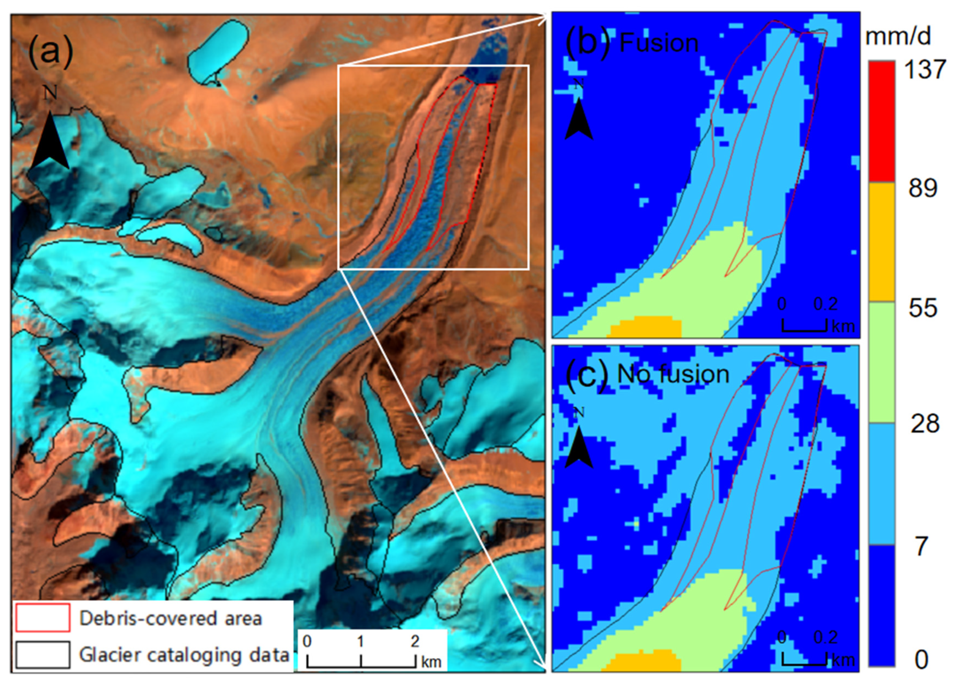
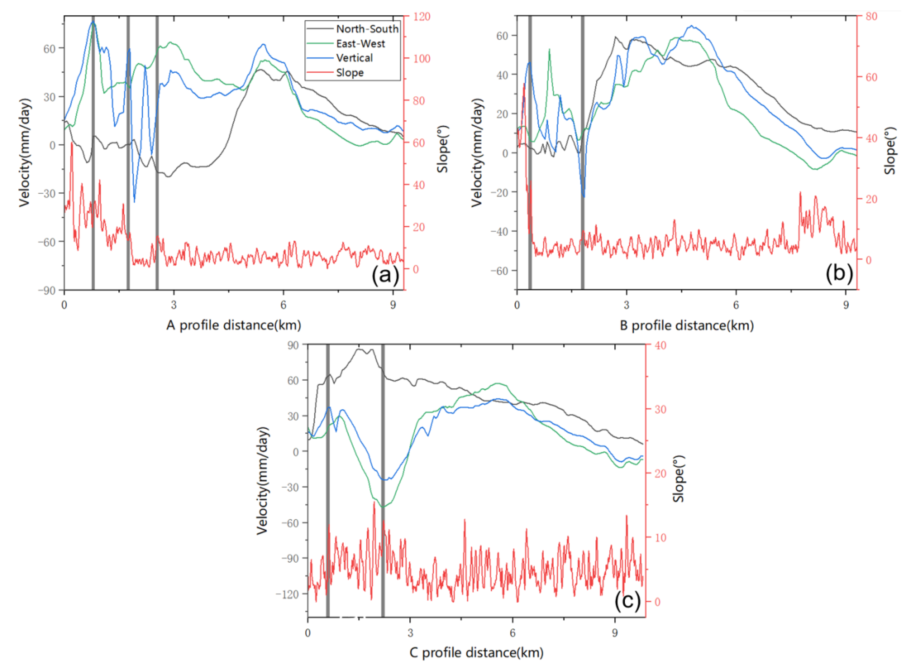
5.3. Factors Affecting Glacier Velocity

The change in glacier velocity is complex [28], and its influencing factors include topographic and meteorological factors [29]. The effect of topographic factors on glacier velocity is mainly shown by the nonlinear positive correlation between the velocity and slope. The larger the slope, the more favorable the glacier movement [30]. The influence of meteorological factors on glacier movement speed is mainly manifested in the thawing of the ice bed caused by temperature rise or the increase in ice temperature and the increase in glacier mobility, which accelerates glacier movement [31]. In the present study, the variation in glacier velocity was analyzed by combining slope and temperature data.

The integrated east–west, north–south, and vertical glacier velocity and slope data were extracted and analyzed (Figure 15) along profiles A, B, and C (Figure 7a). Overall, the slope of the ablation area upstream of the glacier was found to change significantly, and the fluctuation in glacier movement was also significant. Slope changes at 0.79, 1.75, and 2.54 km of profile A led to accelerated glacier movement (Figure 15a). The same case is located at 0.35 and 1.79 km for profile B (Figure 15b) and 0.58 and 2.2 km for profile C (Figure 15c). It is worth noting that the slope of these three profile lines did not change greatly at 5.5 km, but the glacier velocity increased. This phenomenon indicates that there is no absolute positive correlation between glacier velocity and slope. Glacier velocity is also known to be affected by glacier size, glacier thickness, glacier bedrock morphology, and other factors [32]. Generally, the greater the ground slope, the speed of glacier movement will increase accordingly. If the slope is the same, the larger glacier is much faster than the smaller one. The larger the thickness of the glacier is, the greater its static pressure is, and the speed of glacier movement increases. When the bedrock morphology changes, the glacier’s bottom movement may include the sliding on the underlying bedrock and the deformation of the bottom sediment layer.

We compared and analyzed the relationship between optical horizontal time-series deformation and temperature. Points P1, P2, and P3 (Figure 7c) were selected, and the results are shown in Figure 16. Temperature data were obtained from the world weather website (https://rp5.ru/ (accessed on 26 July 2022)). In February 2019, May 2019, and March 2020, the glacier velocity changed significantly with an increase in temperature. In December 2019 and January 2020, the temperature was low, and the glacier velocity changed a negligible amount. From this, we inferred that temperature has an effect on glacier movement. Overall, the change in the glacier movement rate was in line with the trend of temperature change. However, the impact of temperature is not absolute. From the slower movement of glaciers in April 2019 and May 2020 in Figure 16, we show that the movement of glaciers in time may be affected by other factors, such as precipitation.

6. Conclusions

The multi-dimensional and high-precision monitoring of glacier surface velocity variation can provide support for the identification and early warning of glacier disasters. Therefore, in this study, SAR and optical image offset results from 2019 to 2020, combined with the variance component estimation model, were used to jointly solve the three-dimensional flow velocity of a glacier in the central Himalayan region. To this end, the spatial and temporal movement characteristics of the glaciers calculated jointly were analyzed. The results showed that the estimation model based on the variance component obtained cross-platform offset fusion results of heterogeneous data sources and obtained optimal glacier 3D deformation rate results. Compared with the optical results, the accuracy of the fusion results was improved by 41% and 36% in the west–east and south–north directions, respectively. Moreover, the moraine glacier region after fusion was more consistent with the vector boundary of the glacier cataloging data. The fusion results provided higher temporal resolution and more surface velocity information, especially in the area of glacier ablation, where the characteristics of glacier time-series change can be better reflected. At the same time, the monitoring results showed that the maximum displacement rate of the glacier in the east–west, north–south, and vertical directions reached 85, 126, and 88 mm/day, respectively.

The joint solution model has the advantage of the fusion of SAR offset and optical offset, as well as the ability to obtain the local velocity information of the glacier ablation area. However, the joint solution in the vertical direction was completely derived from the decomposition of the SAR offset results. Therefore, the integration of multi-track and multi-platform remote sensing data to improve the accuracy of glacier surface vertical velocity will be investigated in future studies.

References

1. Ding, Y.; Liu, S.; Li, J.; Shangguan, D. The retreat of glaciers in response to recent climate warming in western China. Ann. Glaciol. 2006, 43, 97–105. [Google Scholar] [CrossRef] [Green Version]
2. Raup, B.; Kääb, A.; Kargel, J.S.; Bishop, M.P.; Hamilton, G.; Lee, E.; Paul, F.; Rau, F.; Soltesz, D.; Khalsa, S.J.; et al. Remote sensing and GIS technology in the Global Land Ice Measurements from Space (GLIMS) Project. Comput. Geosci. 2007, 33, 104–125. [Google Scholar] [CrossRef]
3. Rignot, E.; Mouginot, J.; Scheuchl, B. Ice Flow of the Antarctic Ice Sheet. Science 2011, 333, 1427–1430. [Google Scholar] [CrossRef] [PubMed] [Green Version]
4. Kumar, V.; Venkataraman, G.; Høgda, K.A.; Larsen, Y. Estimation and validation of glacier surface motion in the northwestern Himalayas using high-resolution SAR intensity tracking. Int. J. Remote Sens. 2013, 34, 5518–5529. [Google Scholar] [CrossRef]
5. Singh, D.K.; Thakur, P.K.; Naithani, B.P.; Dhote, P.R. Spatio-temporal analysis of glacier surface velocity in dhauliganga basin using geo-spatial techniques. Environ. Earth Sci. 2021, 80, 11. [Google Scholar] [CrossRef]
6. Yang, C.; Lu, Z.; Zhang, Q.; Zhao, C.; Peng, J.; Ji, L. Deformation at longyao ground fissure and its surroundings, north China plain, revealed by ALOS PALSAR PS-InSAR. Int. J. Appl. Earth Obs. Geoinf. 2018, 67, 1–9. [Google Scholar] [CrossRef]
7. Zhang, X.; Zhao, X.; Ge, D.; Liu, B. Motion Characteristics of the South Inilchek Glacier Derived from New C-band SAR Satellite. Geomat. Inf. Sci. Wuhan Univ. 2019, 44, 429–435. [Google Scholar] [CrossRef]
8. Vijay, S.; Khan, S.A.; Kusk, A.; Solgaard, A.M.; Moon, T.; Bjørk, A.A. Resolving Seasonal Ice Velocity of 45 Greenlandic Glaciers With Very High Temporal Details. Geophys. Res. Lett. 2019, 46, 1485–1495. [Google Scholar] [CrossRef] [Green Version]
9. Li, J.; Li, Z.-W.; Wu, L.-X.; Xu, B.; Hu, J.; Zhou, Y.-S.; Miao, Z.-L. Deriving a time series of 3D glacier motion to investigate interactions of a large mountain glacial system with its glacial lake: Use of Synthetic Aperture Radar Pixel Offset-Small Baseline Subset technique. J. Hydrol. 2018, 559, 596–608. [Google Scholar] [CrossRef]
10. Dehecq, A.; Gourmelen, N.; Trouve, E. Deriving large-scale glacier velocities from a complete satellite archive: Application to the Pamir–Karakoram–Himalaya. Remote Sens. Environ. 2015, 162, 55–66. [Google Scholar] [CrossRef]
11. Berthier, E.; Vadon, H.; Baratoux, D.; Arnaud, Y.; Vincent, C.; Feigl, K.; Rémy, F.; Legrésy, B. Surface motion of mountain glaciers derived from satellite optical imagery. Remote Sens. Environ. 2005, 95, 14–28. [Google Scholar] [CrossRef]
12. Bontemps, N.; Lacroix, P.; Doin, M.-P. Inversion of deformation fields time-series from optical images, and application to the long term kinematics of slow-moving landslides in Peru. Remote Sens. Environ. 2018, 210, 144–158. [Google Scholar] [CrossRef]
13. Gray, L. Using multiple RADARSAT InSAR pairs to estimate a full three-dimensional solution for glacial ice movement. Geophys. Res. Lett. 2011, 38. [Google Scholar] [CrossRef]
14. Liu, Y.; Liu, J.; Xia, X.; Bi, H.; Huang, H.; Ding, R.; Zhao, L. Land subsidence of the Yellow River Delta in China driven by river sediment compaction. Sci. Total Environ. 2021, 750, 142165. [Google Scholar] [CrossRef] [PubMed]
15. Ao, M.; Zhang, L.; Liao, M.S.; Zhang, L. Deformation monitoring with adaptive integration of multi-source InSAR data based on variance component estimation. Chin. J. Geophys.-Chin. Ed. 2020, 63, 2901–2911. [Google Scholar] [CrossRef]
16. Hu, J.; Liu, J.; Wu, L.X.; Li, Z.W.; Sun, Q. Integration of Heterogeneous InSAR Measurements for Mapping Complete and Accurate Three-Dimensional Surface Displacements: A Case Study of 2016 Mw 7.8 Kaiköura Earthquake, New Zealand. In Proceedings of the Progress in Electromagnetics Research Symposium (PIERS-Toyama), Toyama, Japan, 1–4 August 2018; pp. 1460–1465. [Google Scholar] [CrossRef]
17. Liu, J.; Zhao, J.; Li, Z.; Yang, Z.; Yang, J.; Li, G. Three-Dimensional Flow Velocity Estimation of Mountain Glacier Based on SAR Interferometry and Offset-Tracking Technology: A Case of the Urumqi Glacier No.1. Water 2022, 14, 1779. [Google Scholar] [CrossRef]
18. Su, Z.; Orlov, A.B. A brief study on the Sino-Soviet Union Shishapangma Glacier in 1991. J. Glaciol. Geocryol. 1992, 184–186. Available online: http://www.bcdt.ac.cn/CN/Y1992/V14/I2/184 (accessed on 26 July 2022).
19. Li, H.; Yang, C.; Hui, W.; Zhu, S.; Zhang, Q. Changes of glaciers and glacier lakes in alpine and extremely alpine regions using remote sensing technology: A case study in the Shisha Pangma area of southern Tibet. Chin. J. Geol. Hazard Control 2021, 32, 10–17. [Google Scholar] [CrossRef]
20. Jiang, S.; Nie, Y.; Liu, Q.; Wang, J.; Liu, L.; Hassan, J.; Liu, X.; Xu, X. Glacier Change, Supraglacial Debris Expansion and Glacial Lake Evolution in the Gyirong River Basin, Central Himalayas, between 1988 and 2015. Remote Sens. 2018, 10, 986. [Google Scholar] [CrossRef] [Green Version]
21. Zhang, G.; Bolch, T.; Allen, S.; Linsbauer, A.; Chen, W.; Wang, W. Glacial lake evolution and glacier–lake interactions in the Poiqu River basin, central Himalaya, 1964–2017. J. Glaciol. 2019, 65, 347–365. [Google Scholar] [CrossRef]
22. Zhang, L.; Liao, M.; Feng, G.; Dong, J.; Ao, M.; Yu, Y. Quantifying the spatio-temporal patterns of dune migration near Minqin Oasis in northwestern China with time series of Landsat-8 and Sentinel-2 observations. Remote Sens. Environ. 2019, 236, 111498. [Google Scholar] [CrossRef]
23. Berardino, P.; Fornaro, G.; Lanari, R.; Sansosti, E. A new algorithm for surface deformation monitoring based on small baseline differential SAR interferograms. IEEE Trans. Geosci. Remote Sens. 2002, 40, 2375–2383. [Google Scholar] [CrossRef] [Green Version]
24. Kong, F.; Qiang, G.; Wang, W. Comparison of four ice velocity measurement software based on optical remote sensing images. Highlights Sci. Online 2016, 9, 1240–1252. Available online: https://www.nstl.gov.cn/paper_detail.html?id=a6956a13978596f39ca155a6562096c1 (accessed on 26 July 2022).
25. Liu, L.; Song, H.; Du, Y.; Feng, G.; Liu, Q.; Sun, M. Time-Series Offset Tracking of the Baige Landslide Based on Sentinel-2 and Landsat 8. Geomat. Inf. Sci. Wuhan Univ. 2021, 46, 1461–1470. [Google Scholar]
26. Hu, J. Theory and Method of Estimating Three-Dimensional Displacement with InSAR Based on the Modern Surveying Adjustment. Ph.D. Thesis, Central South University, CNKI, Changsha, China, 2013. [Google Scholar]
27. Ran, W.; Wang, X.; Guo, W.; Zhao, H.; Zhao, X.; Liu, S.; Wei, J.; Zhang, Y. Glacier cataloging dataset in western China, 2017-2018. China Sci. Data 2021, 6, 195–204. [Google Scholar]
28. Guan, W.; Cao, B.; Pan, B. Research of glacier flow velocity: Current situation and prospects. J. Glaciol. Geocryol. 2020, 42, 1101–1114. [Google Scholar]
29. Xiong, J.; Fan, X.; Dou, X.; Yang, Y. Seasonal variation of velocity of Yarong glacier in Ranwu Lake Basin, Southeast Tibet. Geomat. Inf. Sci. Wuhan Univ. 2021, 46, 1579–1588. [Google Scholar] [CrossRef]
30. Li, J.; Li, Z.; Wang, C.; Zhu, J.; Ding, X. Estimation of the movement of Yinericek Glacier in the south of Tianshan by SAR offset tracking technique. Chin. J. Geophys.-Chin. Ed. 2013, 56, 1226–1236. [Google Scholar]
31. Wang, X.; Liu, Q.; Jiang, L.; Liu, S.; Ding, Y.; Jiang, Z. Characteristics of glacier velocity and its influencing factors in Mount Qomolangma region of the Himalayas based on SAR images. J. Glaciol. Geocryol. 2015, 37, 570–579. [Google Scholar]
32. Jing, Z.; Zhou, Z.; Liu, L. Progress of the Research on Glacier Velocities in China. J. Glaciol. Geocryol. 2010, 32, 749–754. [Google Scholar]
Figure 1. (a) Data coverage map of the experimental area and (b) false color image of the glacier with Landsat 8 OLI Data (652-band Fake Color Synthesis). In (a), the study area is located near Shishapangma Peak in Nyalam County, Tibet Autonomous Region, China, and about 16 km from the China-Nepal border. In (b), blueish colors represent glacier and snow-covered areas, and reddish colors represent bare surface and surface moraine glacier areas.
Remotesensing 15 00004 g001
Figure 2. Technical flow chart of the data processing.
Remotesensing 15 00004 g002
Figure 3. Spatial and temporal baseline combination of SAR images.
Remotesensing 15 00004 g003
Figure 4. Landsat 8 image pairs and their angle difference. (a) Difference between the solar altitude angle and solar azimuth angle for each image pair. (b) Time baseline for each image pair.
Remotesensing 15 00004 g004
Figure 5. Geometric relation of ascending SAR image (arrow direction is positive).
Remotesensing 15 00004 g005
Figure 6. Results of the three-dimensional displacement rate of glacier surface: (a) west–east; (b) north–south; (c) vertical; (d) after the synthesis. The superimposed background is a 3D model from Landsat 8 images combined with DEM in the study area. The upper part of the glacier has reached 6588 meters, with several steep peaks. White shows the snow and glacier-covered area.
Remotesensing 15 00004 g006
Figure 7. Two-dimensional deformation rates of glaciers before and after fusion in the study area: (a) west–east deformation rate after fusion; (b) north–south deformation rate after fusion; (c) optical east–west deformation rate before fusion; (d) optical north–south deformation rate before fusion.
Remotesensing 15 00004 g007
Figure 8. Glacial flow rate difference before and after fusion in the study area: (a) west–east difference of deformation rate; (b) north–south difference of deformation rate.
Remotesensing 15 00004 g008
Figure 9. Profiles of glacial flow rate before and after fusion: (a,c,e) west–east flow velocity profiles along A, B, and C (Figure 7); (b,d,f) south–north flow velocity profiles along A, B, and C.
Remotesensing 15 00004 g009
Figure 10. Monitoring accuracy before and after fusion: (a) stable regions R1, R2, and R3 for accuracy assessment; (b) standard deviation comparison in the west–east stable region; (c) standard deviation comparison in the north–south stable region.
Remotesensing 15 00004 g010
Figure 11. Comparison of glacier cataloging information and joint results in the study area. (a) Cataloging glacier data and mapping areas covered by moraines; (b) The fusion results are more consistent with the surface moraine glacier boundary; (c) The result without fusion was inconsistent with the surface moraine glacier boundary.
Remotesensing 15 00004 g011
Figure 12. West–east time-series glacier velocity in the study area.
Remotesensing 15 00004 g012
Figure 13. North–south time-series glacier velocity in the study area.
Remotesensing 15 00004 g013
Figure 14. Vertical time-series glacier velocity in the study area.
Remotesensing 15 00004 g014
Figure 15. Comparison of profiles for glacier velocity and topographic profile (profiles along A, B, and C are shown in Figure 7a). (a) Deformation velocity and slope of profile A; (b) Deformation velocity and slope of profile B; (c) Deformation velocity and slope of profile C.
Remotesensing 15 00004 g015
Figure 16. Relationship between optical horizontal time-series deformation and temperature in the glacial study area (error bar is calculated as 5% of the data). P1, P2, and P3 are shown in Figure 7c. The average monthly temperature data are from the Xigaze weather station on the world weather website (https://rp5.ru/ (accessed on 26 July 2022)).
Remotesensing 15 00004 g016