Article

Mapping Forest Growing Stem Volume Using Novel Feature Evaluation Criteria Based on Spectral Saturation in Planted Chinese Fir Forest

1
Research Center of Forestry Remote Sensing and Information Engineering, Central South University of Forestry and Technology, Changsha 410004, China
2
Key Laboratory of Forestry Remote Sensing Based Big Data and Ecological Security for Hunan Province, Changsha 410004, China
3
Key Laboratory of State Forestry Administration on Forest Resources Management and Monitoring in Southern Area, Changsha 410004, China
4
Department of Land Surveying and Geo-Informatics, The Hong Kong Polytechnic University, Hung Hom, Kowloon, Hong Kong, China
5
Soil Science Department, Lorestan University, Khoramabad 68151-44316, Iran
*
Author to whom correspondence should be addressed.
Submission received: 21 November 2022 / Revised: 3 January 2023 / Accepted: 5 January 2023 / Published: 10 January 2023
(This article belongs to the Collection Feature Paper Special Issue on Forest Remote Sensing)

Abstract

:
Forest growing stem volume (GSV) is regarded as one of the most important parameters for the quality evaluation and dynamic monitoring of forest resources. The accuracy of mapping forest GSV is highly related to the employed models and involved remote sensing features, and the criteria of feature evaluation severely affect the performance of the employed models. However, due to the linear or nonlinear relationships between remote sensing features and GSV, widely used evaluation criteria inadequately express the complex sensitivity between forest GSV and spectral features, especially the saturation levels of features in a planted forest. In this study, novel feature evaluation criteria were constructed based on the Pearson correlations and optical saturation levels of the alternative remote sensing features extracted from two common optical remote sensing image sets (GF-1 and Sentinel-2). Initially, the spectral saturation level of each feature was quantified using the kriging spherical model and the quadratic model. Then, optimal feature sets were obtained with the proposed criteria and the linear stepwise regression model. Finally, four widely used machine learning models—support vector machine (SVM), multiple linear stepwise regression (MLR), random forest (RF) and K-neighborhood (KNN)—were employed to map forest GSV in a planted Chinese fir forest. The results showed that the proposed feature evaluation criteria could effectively improve the accuracy of estimating forest GSV and that the systematic distribution of errors between the predicted and ground measurements in the range of forest GSV was less than 300 m3/hm2. After using the proposed feature evaluation criteria, the highest accuracy of mapping GSV was obtained with the RF model for GF-1 images (R2 = 0.49, rRMSE = 28.67%) and the SVM model for Sentinel-2 images (R2 = 0.52, rRMSE = 26.65%), and the decreased rRMSE values ranged from 1.1 to 6.2 for GF-1 images (28.67% to 33.08%) and from 2.3 to 6.8 for Sentinel-2 images (26.85% to 33.28%). It was concluded that the sensitivity of the optimal feature set and the accuracy of the estimated GSV could be improved using the proposed evaluation criteria (less than 300 m3/hm2). However, these criteria were barely able to improve mapping accuracy for a forest with a high GSV (larger than 300 m3/hm2).

Graphical Abstract

1. Introduction

Forest growing stem volume (GSV), widely applied in forest resource investigations, is regarded as one of the most important indices in forest resource quality evaluation [1,2,3]. Traditional approaches of mapping forest GSV need a lot of field investigation [4,5,6]. In recent years, remote sensing technology has become one of the most important methods used to estimate forest parameters, such as forest height, GSV and above ground biomass (AGB) [7,8]. In particular, optical remote sensing images with rich data resources are widely applied to evaluate forest types and quantitatively estimate forest parameters [9,10]. Normally, optical remote sensing images reflect the forest growth process and changes in the forest canopy information, and the spectral variables extracted from optical image sets, including Landsat, Sentinel-2, GF-1, and GF-2, are often used to construct models for mapping GSV. However, these variables are insensitive to changes in GSV when the GSV is larger than the saturation levels. Previous studies also proved that the accuracy of mapping GSV using optical images is affected by an underestimated GSV because of the saturation phenomenon [11,12]. Therefore, it is still difficult to obtain reliable GSV using optical images in plantation forests with high GSV levels.
To improve the accuracy of GSV mapping, underestimated GSV should be corrected by delaying saturation levels by selecting appropriate feature sets [13]. Generally, it has been proved that a forest’s vertical structure parameters are more sensitive to GSV than forest canopy information [14]. Previous studies have explored various methods to extract vertical forest parameters by delaying the saturation phenomenon, such as synthetic aperture radar (SAR) or polarimetric SAR data, airborne or spaceborne light detection and ranging (LiDAR), and CHM products generated from stereo image pairs [15,16,17,18]. Though some results have showed that saturation levels can be delayed by adding vertical forest parameters, airborne LiDAR is not suitable for assessing forest height over large regions because of the high cost of acquiring data [19,20]. In addition, for orbital LiDAR data, the accuracy of forest height in light spots rarely meets the requirements for forest parameter estimation in medium-scale regions. Therefore, optical remote sensing images remain the main source of data for mapping forest parameters.
Furthermore, feature evaluation criteria are also important for improving underestimated or overestimated results in mapping forest GSV [21,22,23]. Normally, optical variable sets are rather dependent on the employed evaluation metrics, and the accuracy of estimated GSV is also highly related to the sensitivity of selected variables [24]. Generally, feature evaluation methods are mainly based on the linear or nonlinear relationships between remote sensing features and GSV, such as importance, distance correlation coefficient (DC), maximal information coefficient (MIC), and Pearson correlation coefficient [7,25,26,27]. However, these inadequately express the sensitivity between forest GSV and spectral features, especially for the planted forest with a high GSV. After all, underestimated forest GSVs are mainly caused by the spectral saturation phenomenon that occurs when using optical remote sensing images.
Additionally, optimal feature sets are obtained with various feature selection methods. Commonly, the feature selection methods can be broadly classified into three categories: filters, wrappers, and embedded. Filters are entirely based on a single evaluation criterion, such as importance or Pearson correlation. However, determining this criterion and its threshold is rather difficult for various sensors and features [28,29]. Wrappers combine the feature selection methods with training models, and then, an optimal feature set is extracted with a certain accuracy index and repeatedly trained models [30,31]. However, these feature selection methods only refer to a single criterion, such as linear independence, information entropy, or precision index, and the saturation level of each variable is not considered as an evaluating feature method [32,33]. Therefore, to correct an underestimated GSV, the saturation levels of alternative variables should be viewed as a criterion to evaluate the sensitivity between the variables and GSV [34,35,36]. In addition, because the kriging spherical model and the quadratic model are gradually being applied to quantitatively evaluate the saturation levels of the features extracted from remote sensing images, it is more advantageous to focus on spectral saturation in feature evaluation and selection [37,38].
To overcome the disadvantages of traditional feature evaluation criteria in mapping forest GSV, we constructed novel feature evaluation criteria based on the Pearson correlations and optical saturation levels of each alternative remote sensing feature. In this study, two widely used optical remote sensing image sets, GF-1 and Sentinel-2, were acquired from a planted Chinese Fir Forest, and several types of common features, bands, vegetation indices, and texture features with different sizes were extracted from the acquired images. Then, the saturation level of each extracted feature was estimated using the kriging spherical model and the quadratic model. Next, the proposed feature evaluation criteria were constructed and applied to obtain optimal feature sets for mapping forest GSV with four models: the support vector machine (SVM), multiple linear regression (MLR), random forest (RF), and K-nearest neighbor (KNN) models. The capability of the new feature evaluation criteria was further evaluated with accuracy indices for mapping forest GSV.

2. Study Area and Data
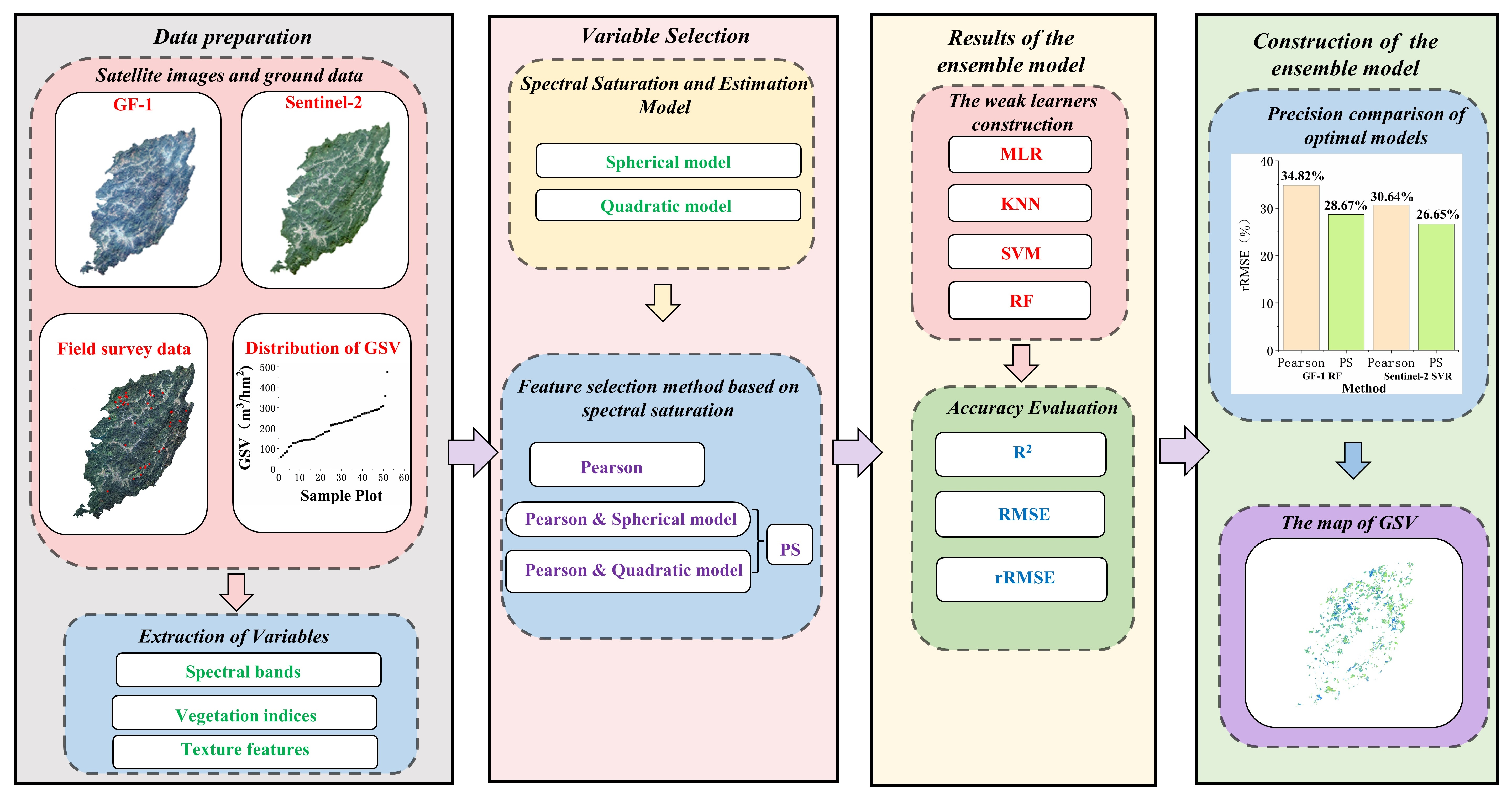
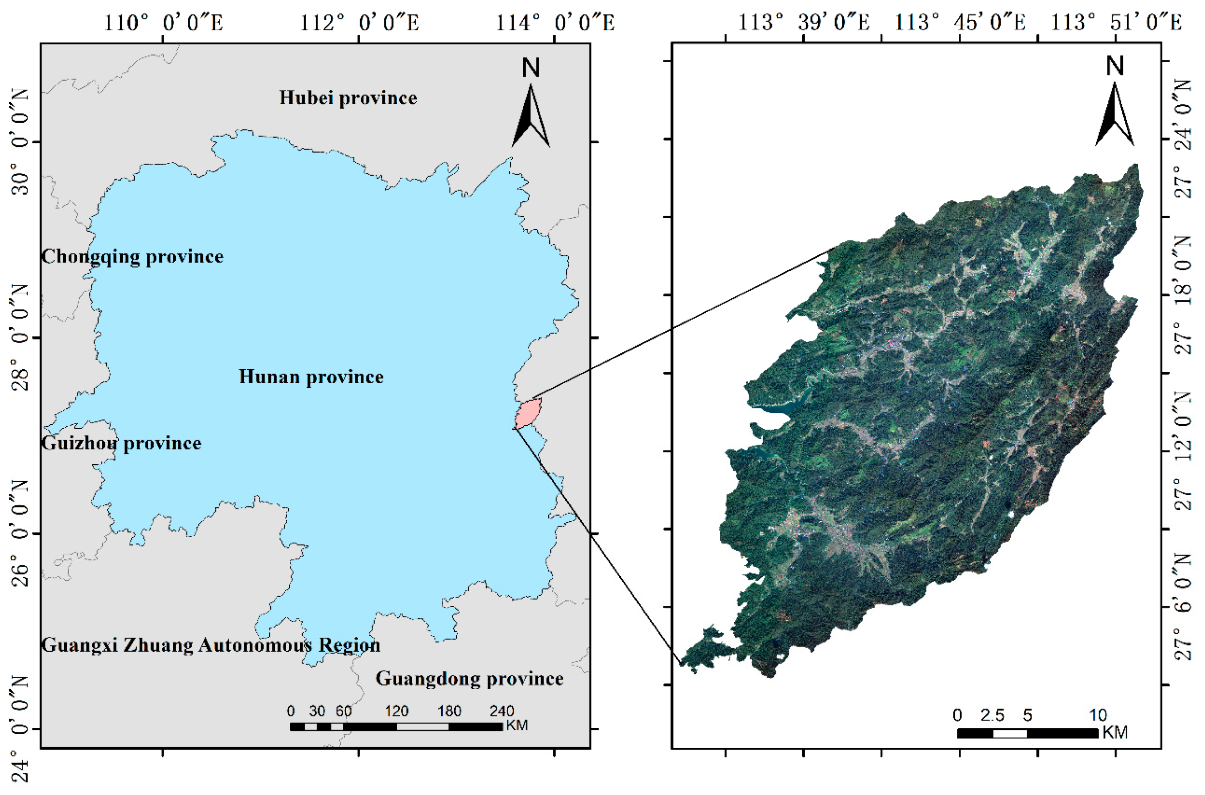
2.1. Study Area

In this study, the Huangfengqiao state-owned forest farm (113°04′ to 113°43′E, 27°06′ to 27°24′N), located in You County, Hunan province, China, was selected as the study area. The landform of the forest farm is mainly low and middle mountains, with the elevation ranging from 115 m to 1270 m and the slope ranging from 20° to 35°. The climate type of the region is a subtropical monsoon humid climate, and the annual mean temperature and the average annual rainfall are 17.8 °C and 1410.8 mm, respectively. The forest coverage rate reaches 86.24% in the region (10,122.6 ha) and comprises Chinese fir (Cunninghamia Lanceolata), Pinus massoniana Lamb, bamboo, and Liriodendron chinense. The planted Chinese fir is the dominant species in the study area (Figure 1).

2.2. Data Preparation

(1)
Ground Data
Because of the irregular distribution of the planted Chinese fir forest, a random stratification sampling method was used to obtain the distribution of the ground samples. Then, a total of 52 Chinese fir plots were measured during field investigations in 2016 and 2017 (Figure 2a). For all ground samples, the size of each sample (Including 19 plots of 20 m × 20 m and 33 plots of 30 m × 30 m) was determined by the complexity of the terrain. Moreover, the positions of the corner and central points of samples were accurately measured using a global positioning system (GPS) (positioning error of less than 10 cm). In each sample, parameters related to forest GSV were measured in ground field work, tree height was measured using a laser altimeter, diameter at breast height (DBH) was measured with a diameter ruler, and crown width in the east–west and north–south directions was measured with a tape. The stem volume of each tree was calculated based on the binary volume table of planted Chinese fir in Hunan province (Equation (1)), and the GSV of each sample was the sum of all tree stem volumes within the plot. In the study, the maximum DBH and height were 29.48 cm and 20.5 m, respectively. The GSV of the measured samples ranged from 59 m3/hm2 to 480 m3/hm2, and relationships between forest GSV and DBH are plotted in Figure 2b.
V = a × D B H b × H c
where V is the volume of each tree, a = 0.000058777042, b = 1.9699831, and c = 0.89646157.
(2)
Remote sensing data and pre-processing
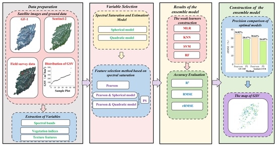
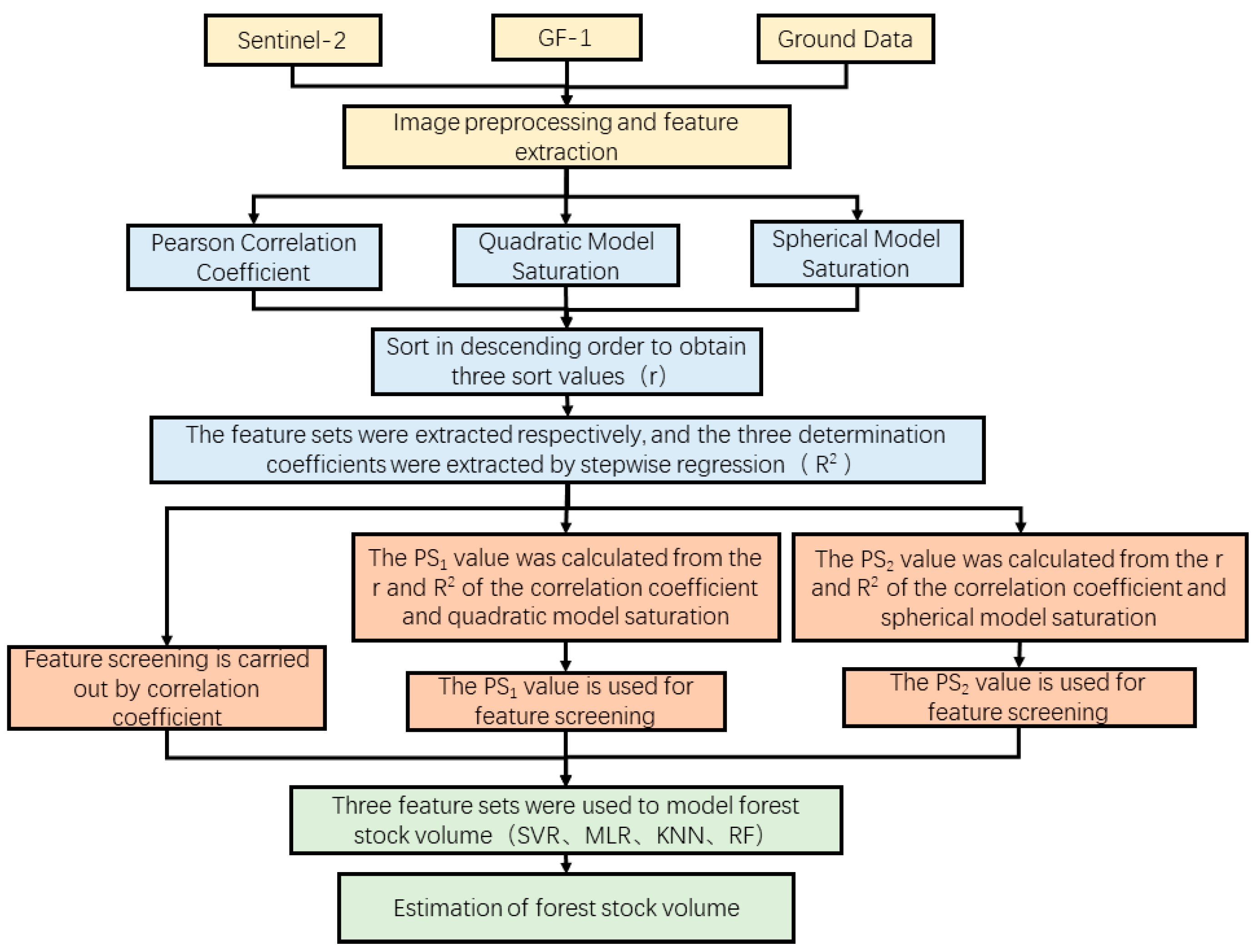
In this study, two remote sensing image sets, GF-1 and Sentinel-2, were employed to map the forest GSV in a planted Chinese fir forest. Specially, GF-1 images with 4 multispectral bands (spatial resolution: 8 m) and 1 panchromatic band (spatial resolution: 2 m), were acquired on 29 July 2016 (Table 1). Meanwhile, Sentinel-2 images with 13 narrow bands were acquired on 1 November 2017, and the spatial resolution of these bands was 10 m, 20 m and 60 m [39]. To extract alternative variables from these remote sensing images, a series of pre-processing steps, including radiometric calibration, atmospheric correction, ortho-correction, geometric correction, image fusion, and clipping, were applied to the GF-1 and Sentinel-2 images [40]. The preprocessing of remote sensing data was implemented in ENVI 5.3 software. Ultimately, these pre-processed images were resampled to 30 m to reduce the matching error between images and samples.

3. Methods

3.1. Extracting Features

After image preprocessing, three types of features (spectral bands, vegetation indices, and texture features) were extracted from GF-1 and Sentinel-2 images (Table 2). In our study, the number of spectral bands was four for GF-1 images and eleven for Sentinel-2 images. Additionally, several texture features with different sizes were extracted from each spectral band using a gray-level co-occurrence matrix (GLCM). Considering the difference in spatial resolutions, the sizes of the extracted texture features ranged from 3 × 3 to 19 × 19. Moreover, several vegetation indices were also extracted from these images [41,42].

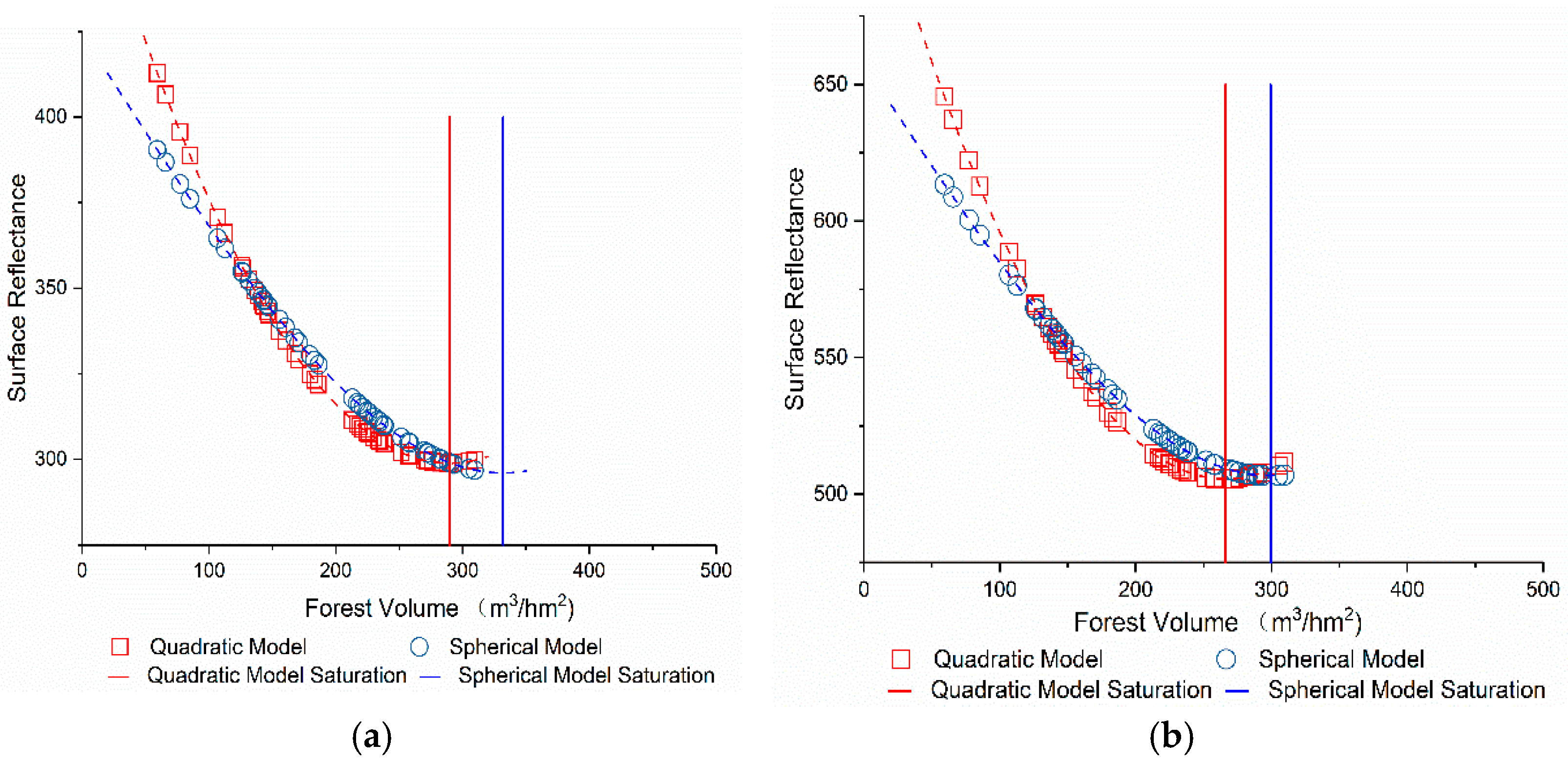
3.2. Spectral Saturation and Estimation Model

In previous studies, saturation levels were indirectly obtained from extreme values based on scatterplots or fitted curves between selected variables and GSV via visual interpretation. Over the past ten years, some models related to saturation levels have been applied to determine saturation levels [46,47,48]. In particular, a semi-exponential model has often been employed to estimate saturation levels using SAR or polarimetric SAR images, and the saturation level can be directly extracted from parameter models after solving them [18,43,44,45]. For optical images, a kriging model based on the semi-covariance function in geo-statistics has been widely applied to quantitative analysis spectral saturation. Moreover, it has also been proven that the quadratic model can characterize spectral saturation levels. Therefore, the kriging and quadratic models were applied to evaluate the saturation levels in this study.
(1)
Kriging Model
When the GSV reaches a certain value, the saturation of spectral variables will occur, and the saturation phenomenon has been proved to be similar to the distribution of spatial autocorrelation in geo-statistics [14,38,45]. The kriging model with a spherical function has the capability of describing the phenomenon of spectral saturation related to GSV. In this study, the kriging model with a spherical function was applied to fit the relationships between GSV and the selected variables:
y ( h ) = {   c 0                                                       h = 0 c 0 + c ( 3 h 2 a h 3 2 a 3 ) 0 < h a c 0 + c                                   h > a
where y is the selected spectral variable, h is the value of the GSV, c 0 is the nugget parameter indicating the spectral reflectance value at h = 0, c is arch height indicating the change rates of the spectral reflectance of the selected variable and the GSV, c 0 + c is the maximum or minimum spectral reflectance when the GSV reaches its saturation value, a is the value of saturation related to GSV; when c 3 2 a 3   =   a 2 3 c 2 a = a1, c 0 = a0, x1 = h, and x2 = h3, the spherical model is linearized and its coefficients of linear regression can be obtained using least squares regression:
y = a 2 × x 2 + a 1 × x 1 + a 0
After resolving the linearized model, the saturation level located at the extreme value of the function is calculated according to the model parameters. Combined with the extreme point of the curve of the model, the saturation of the kriging spherical model is expressed as:
s a t u r a t i o n   v a l u e s = a 1 3 a 0
(2)
Quadratic model
The quadratic model has been applied to fit the curves between the GSV and spectral variables. The quadratic model is expressed as follows:
y = a 0 x 2 + a 1 x + a 2
where y is the selected spectral variable, x is the value of the GSV, and a 0 , a 1 , and a 2 are model parameters. After solving the model, the extreme point of the fitted curve is regarded as the saturation value. Therefore, the saturation of the quadratic model is expressed as:
s a t u r a t i o n   v a l u e s = a 1 2 a 0
Based on the spherical and quadratic models, the saturation values and the curves between the estimated GSV and selected spectral variable are illustrated in Figure 3 (band 3 for GF-1 in Figure 3a and band 5 for Sentinel-2 in Figure 3b). It is shown that the estimated saturations of band 3 extracted from GF-1 was 289.68 m3/hm2 for the spherical model and 332.1 m3/hm2 for the quadratic model. Additionally, the estimated saturation of band 5 extracted from Sentinel-2 was 266.25 m3/hm2 for the spherical model and 299.24 m3/hm2 for the quadratic model. Due to the differences in the spectral saturation estimation models, the estimated saturation of the same spectral feature was different.

3.3. Feature Selection Method Based on Spectral Saturation

Normally, the accuracy of mapped forest GSV is directly dependent on the sensitivity of the selected feature set. However, the Pearson correlation coefficient is widely regarded as an important index used to evaluate sensitivity based on linear independence. Moreover, the spectral saturation levels of remote sensing features can directly describe the range of estimated forest GSV. Therefore, the saturation levels of features should also be regarded as an index to evaluate sensitivity. Theoretically, the selected features in an optimal variable set should have high spectral saturation levels and Pearson correlations. Therefore, new feature evaluation criteria were proposed based on the spectral saturation and Pearson correlation coefficient. The steps of the proposed feature evaluation criteria are as follows:
(1) The Pearson correlation coefficient and spectral saturation levels of all extracted remote sensing features related to GSV are first obtained and sorted in descending order.
(2) Based on the sorted Pearson correlation coefficient and spectral saturation levels, the serial numbers r 1 i (Pearson correlation coefficient) and r 2 i (spectral saturation levels) of each feature i   are obtained.
(3) To obtain the initial variable set, a multiple linear stepwise regression model and an adjusted determination coefficient are employed to determine the number of features sorted by the Pearson correlation coefficient and spectral saturation levels, respectively. The initial variable set is determined based on the maximum values of the adjusted determination coefficients R1 (Pearson correlation coefficient) and R2 (spectral saturation levels).
(4) In an initial variable set, a new importance evaluation index (PS: Pearson and saturation) is constructed by using the serial numbers and the determination coefficient with the following formula:
P S i = r 1 i R 1 + r 2 i R 2  
where P S i is the value of the importance evaluation index corresponding to the Pearson correlation coefficient and spectral saturation levels.
(5) Finally, features are sorted by the PS values in descending order; the smaller the PS value, the higher the importance of the feature.

3.4. Model Evaluation and Application

To evaluate the capability of the proposed feature evaluation criteria, the saturation levels of all features were derived from the kriging model with a spherical function and the quadratic model, and optimal feature sets were finally obtained with the Pearson correlation coefficient and the proposed feature selection criteria. Next, four models (SVM, MLR, RF and KNN [41,42,47]) were applied to map the forest GSV using the optimal feature set. The flowchart of mapping GSV is illustrated in Figure 4.
Additionally, the accuracy of the mapped GSV was evaluated with leave-one-out cross-validation (LOOCV). The adjusted determination coefficient (R2), root mean square error (RMSE), and relative root mean square error (rRMSE) between the predicted and ground-measured GSV were selected as the evaluation indices [48].
R 2 = 1 ( 1 [ 1 i = 1 n ( y i y i ^ ) 2 i = 1 n ( y i y i ¯ ) 2 ] 2 ) ( n 1 ) n p 1
R M S E = i = 1 n ( y i y i ^ ) 2 n
r R M S E = R M S E y i ¯ × 100 %
where y i is the measured GSV, y i ^ is the predicted GSV, y i ¯ is the average of the measured GSV, and n is the number of samples.

4. Results

4.1. Saturation Values of Features

To evaluate the sensitivity between GSV and features, the saturation levels of alternative spectral features should first be estimated. In our study, the quadratic model and the spherical model were employed to estimate the saturation values of the features extracted from GF-1 and Sentinel-2 images, respectively (Figure 5 and Table 3). Figure 5 illustrates the fitted curves of the top ten features extracted from GF-1 (Figure 5a,b) and Sentinel-2 (Figure 5c,d) images. For one feature, the curves fitted by the quadratic model and the spherical model were basically the same, and the estimated values of spectral saturation were slightly different. However, the fitted curves and their saturation levels were significantly different for different remote sensing images.
For the top ten features, the absolute values of the Pearson correlation coefficient ranged from 0.45 and 0.65 for the features extracted from GF-1 images and from 0.40 to 0.51 for the features extracted from Sentinel-2 images. Moreover, for the GF-1 images, the saturation levels ranged from 240.78 m3/hm2 to 474.54 m3/hm2 using the quadratic model and from 249.22 m3/hm2 to 474.54 m3/hm2 using the spherical model. For the Sentinel-2 images, the absolute values of the Pearson correlation coefficient between the extracted features and forest GSV ranged from 0.42 to 0.50, and the spectral saturation levels ranged from 283.17 m3/hm2 to 474.54 m3/hm2 using the quadratic model and from 278.36 m3/hm2 to 474.54 m3/hm2 using the spherical model. It was also found that the orders of spectral saturation did not match the orders of the Pearson correlation coefficient. When using the Pearson correlation to select features, the results proved that the optimal feature set ignored the saturation effect. Therefore, it was necessary to retrieve the optimal feature set based on the Pearson correlation and saturation levels.

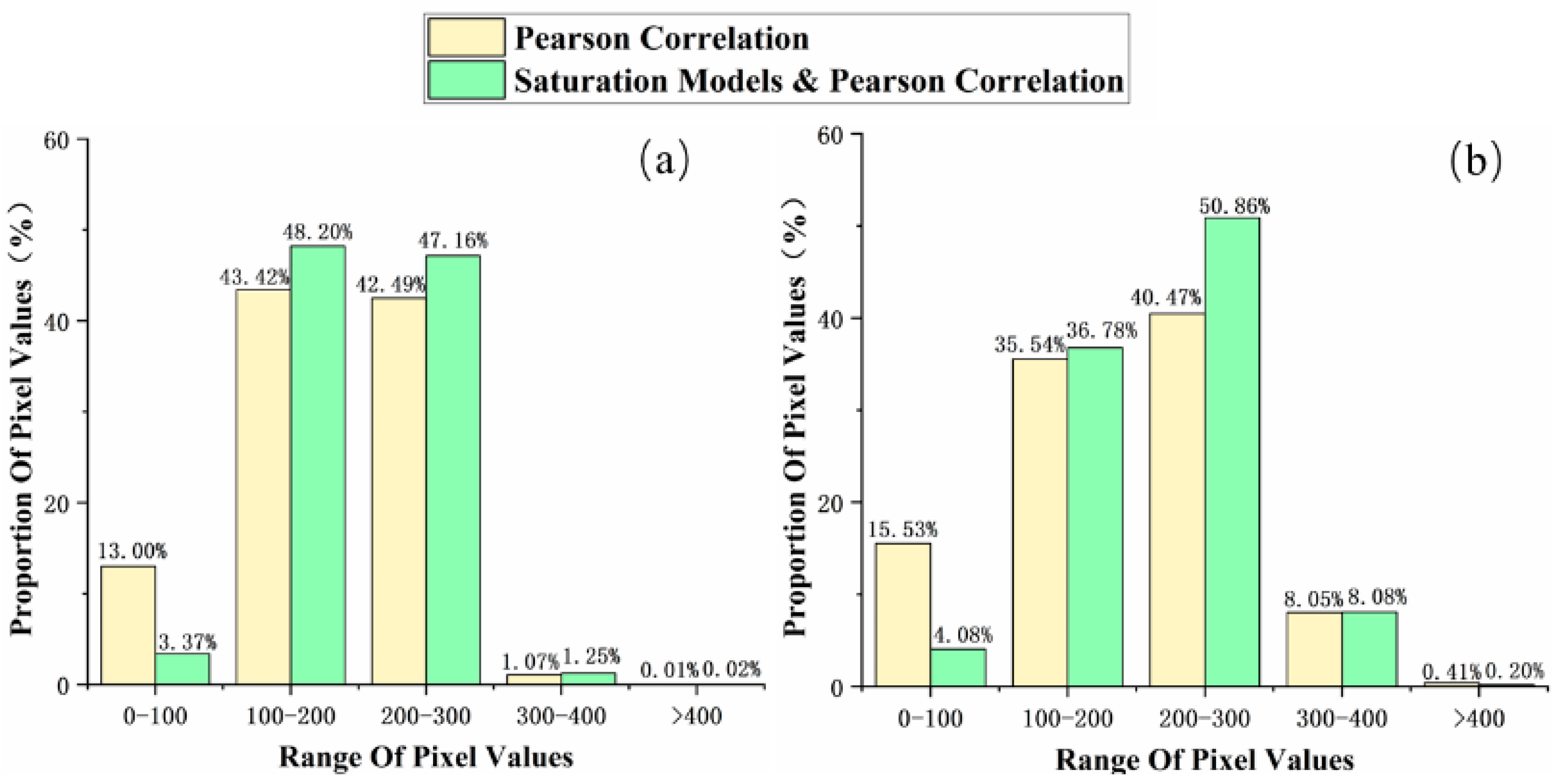
4.2. The Results of Proposed Feature Evaluation Criteria

To obtain the initial feature set, all extracted features were first sorted in descending order according to Pearson correlation and spectral saturation levels. Then, the linear stepwise regression model was employed to calculate the adjusted determination coefficient (R2) for various sorted features. Ultimately, the initial feature set was constructed from the union of the two feature sets extracted from the Pearson correlation and spectral saturation levels w the maximum determination coefficient. In this study, based on Pearson correlations, the saturation level of the quadratic model, and the saturation level of the spherical model, the maximum determination coefficients were 0.412, 0.322, and 0.303 for the GF-1 images and 0.401, 0.302, and 0.319 for the Sentinel-2 images, respectively. Using the proposed feature evaluation criteria, the new importance evaluation index (PS) of the selected features in the initial feature set was constructed using the serial numbers and determination coefficients. The top ten PS values extracted from the GF-1 and Sentinel-2 image sets are listed in Table 4 and Table 5, respectively.
When using the proposed feature evaluation criteria, the PS values of the top 10 variables extracted from the GF-1 images ranged from 17.96 to 45.33 with the quadratic model and from 18.93 to 46.50 with the spherical model. Compared with a single criterion, the PS values between the feature and GSV also contained contributions from the Pearson correlation coefficient and spectral saturation levels. Therefore, the PS values were determined by the orders of the Pearson correlation coefficient and saturation levels. It is illustrated that some features with high Pearson correlation coefficients were excluded from the top 10 variables extracted with the proposed method because of low saturation levels, such as 3B1_VAR extracted from the GF-1 images. Moreover, the values of PS were also related to the employed models used to extract spectral saturation levels. The gaps of estimated spectral saturation levels were mainly induced by the quadratic and spherical models. When using the new criteria, most of the variables were in the top ten, but the orders changed.
For the Sentinel-2 images (Table 5), the orders of the top ten variables evaluated with the proposed method were rather different from those of the variables extracted with Pearson correlation coefficients or spectral saturation levels. After using the proposed method, the ranks of the features changed. Though there were some differences in the estimated saturation values when using the different estimation models, it was found that these models had no effect on the rank of the top ten features when using the proposed feature selection method.

4.3. Optimal Feature Set

Using the linear stepwise regression model and determination coefficients, the initial feature set was formed from the union of the two feature sets extracted from the Pearson correlations and spectral saturation levels with the maximum determination coefficient. Then, the PS values of all initial feature sets were retrieved with the proposed feature selection method. To guarantee the independence of the features, variance inflation factor (VIF) was introduced to conduct collinearity analysis, and refined feature sets were constructed after removing linearly dependent features. Finally, after using linear stepwise regression models, optimal feature sets of various feature selection methods were obtained from the refined feature set in descending order. In our study, three optimal feature sets (Table 6) were derived using Pearson correlation coefficients, PS values with the spherical model, and PS values with the quadratic model. For various feature selection methods, the numbers of features contained in the optimal feature set are largely dependent on the feature selection methods.
For the GF-1 images, the optimal feature set mainly came from texture information, and the number of feature sets was dependent on the FS methods. There were five features in the optimal feature set using Pearson correlations and seven features in the optimal feature set using the proposed method. Furthermore, these optimal feature sets with different models used for estimating saturation levels had the same features. For the Sentinel-2 images, most selected features came from vegetation indices, and the results of the optimal feature set were the same when using different models to estimate the saturation levels. It was inferred that the optimal feature sets obtained from the proposed method were largely dependent on the relative changes in saturation levels.

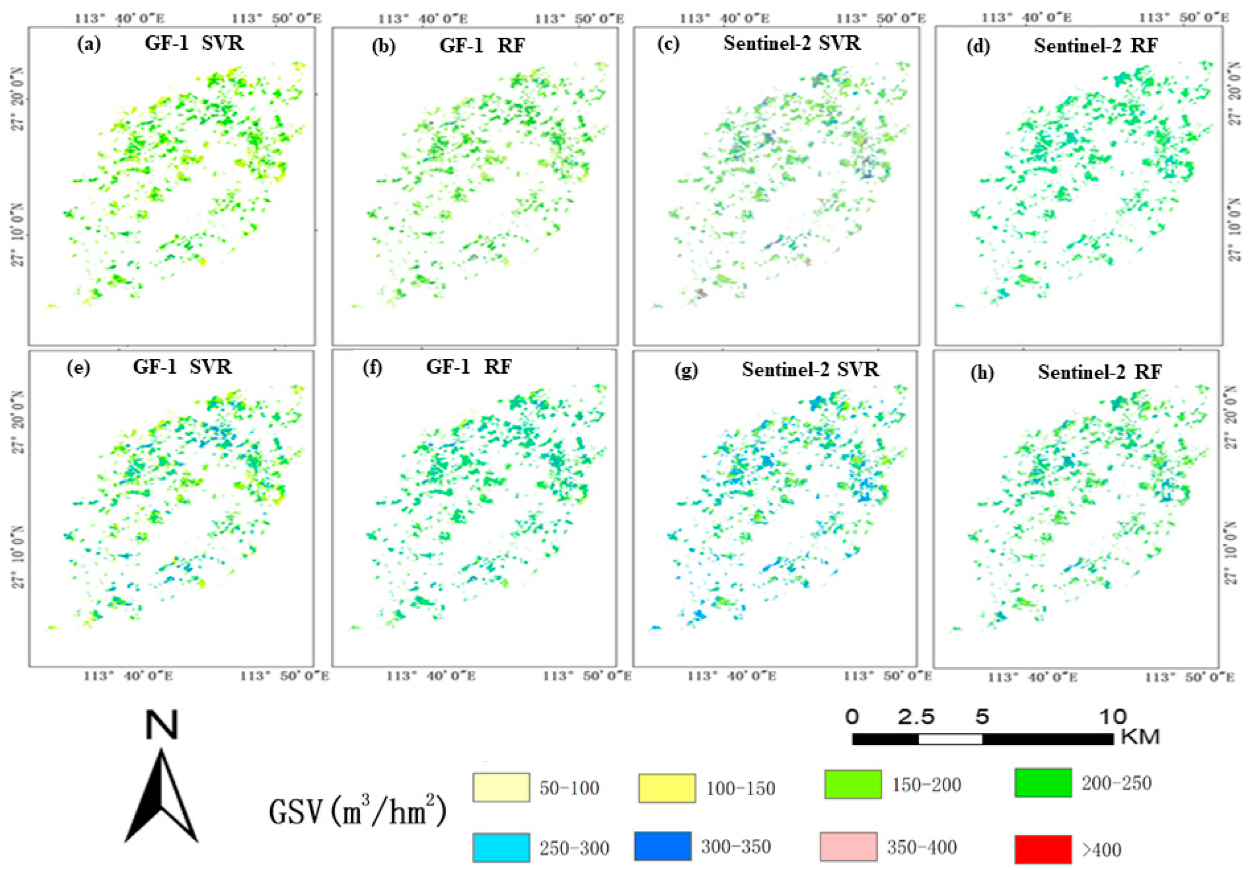
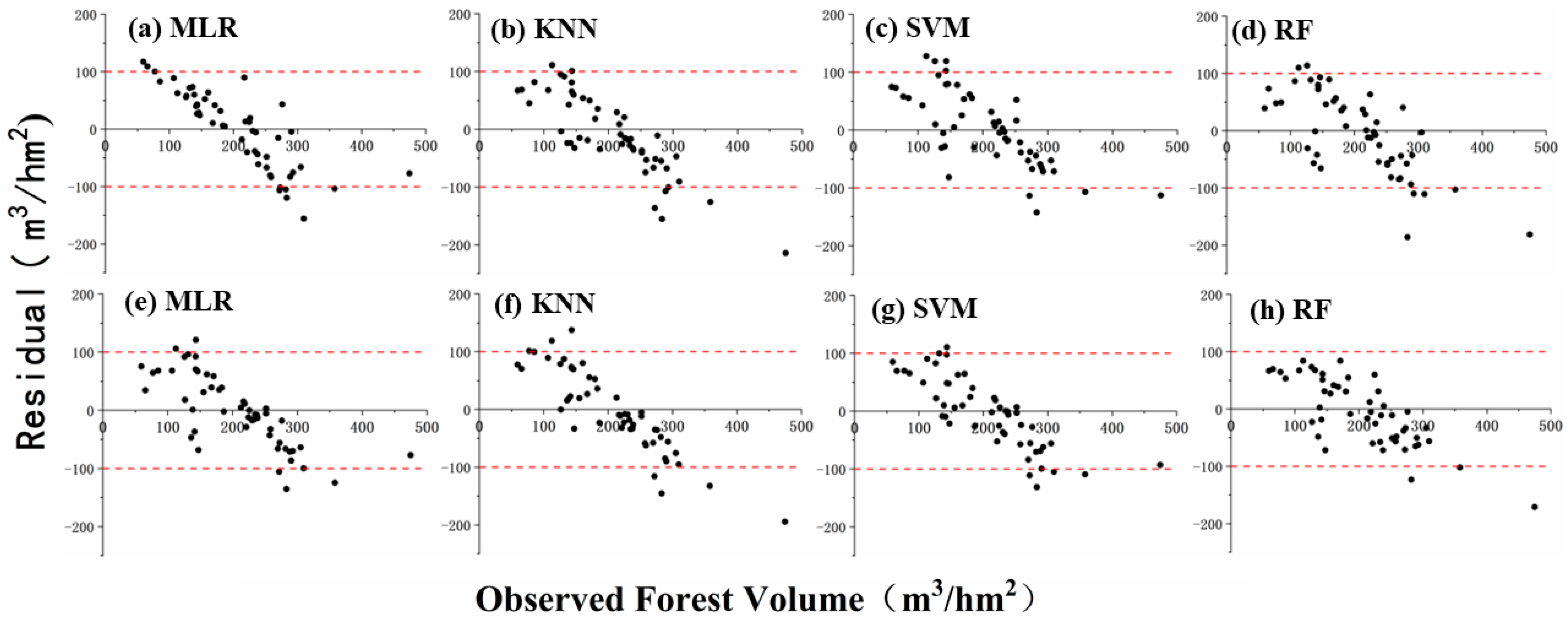
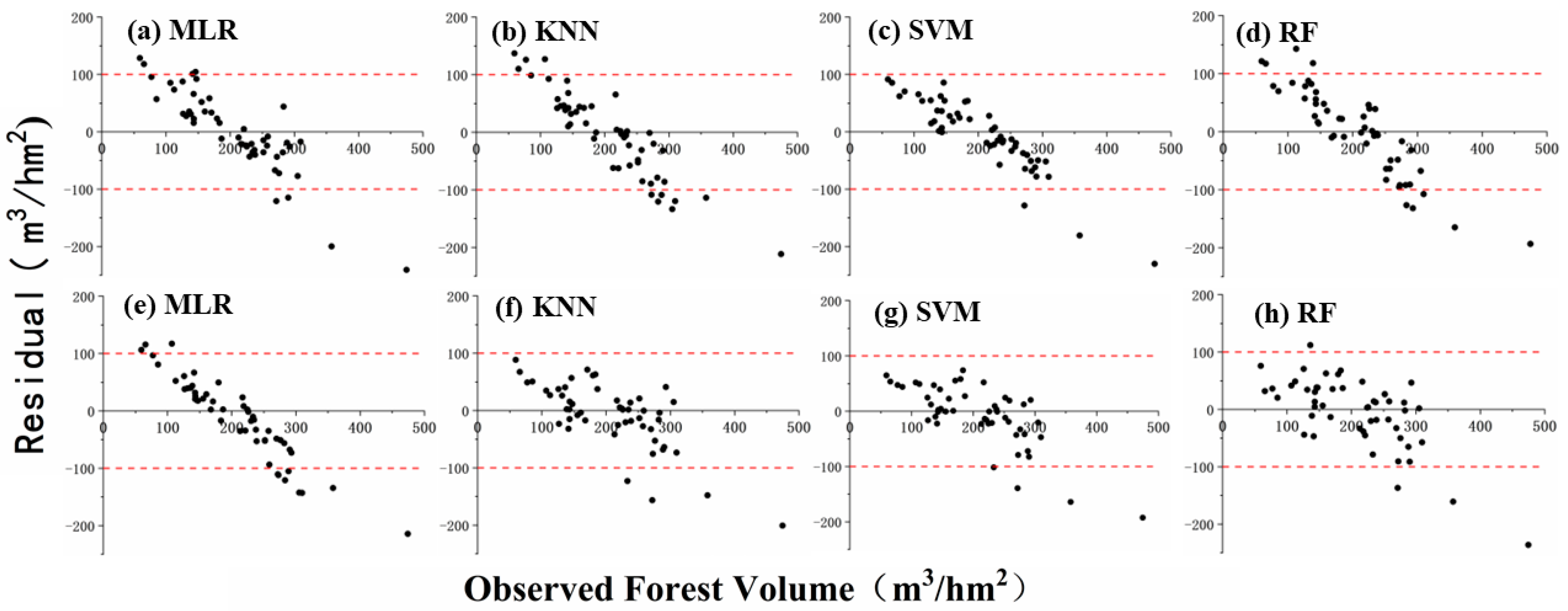
4.4. The Results of Estimated Forest GSV

To further analyze the capability of the proposed feature evaluation criteria, four models (SVM, MLR, RF and KNN) were employed to estimate forest GSV using two optimal feature sets extracted from GF-1 and Sentinel-2 images. LOOCV was used to retrieve the evaluation indices, including the determination coefficient (R2), root mean square error (RMSE), and relative root mean square error (rRMSE) between the predicted and measured GSV values. The estimated results of the four models are listed in Table 7.
Table 7 shows that the proposed feature evaluation criteria could effectively improve the accuracy of estimating forest GSV. When using the optimal feature set obtained with Pearson correlations, the rRMSE values ranged from 32.57% to 34.82% for the GF-1 images and from 30.64% to 36.53% for the Sentinel-2 images. After using the optimal feature set obtained with the proposed feature evaluation criteria, the saturation levels and Pearson correlations between features and GSV were employed to evaluate the capability of the features in mapping GSV. The rRMSE values ranged from 28.67% to 33.08% for the GF-1 images and from 26.85% to 33.28% for the Sentinel-2 images. The highest GSV mapping accuracy was obtained with the RF model for the GF-1 images (R2 = 0.49, rRMSE = 28.67%) and with the SVM model for the Sentinel-2 images (R2 = 0.52, rRMSE = 26.65%). It was obvious that the optimal feature set obtained with the proposed method was better able to map GSV than that obtained with Pearson correlation coefficients.
To further analyze the estimated forest GSV, scatter plots between ground-measured and predicted GSV were plotted using the GF-1 images (Figure 6) and the Sentinel-2 images (Figure 7). It was found that the accuracy of mapping forest GSV relied on the feature evaluation criteria. After using the proposed method, the features were simultaneously evaluated by double criteria, saturation levels and Pearson correlation, and overestimated results with low GSV values were significantly improved by adding some features with high saturation levels to the optimal feature set. Figure 6 and Figure 7 illustrate that the number of underestimated samples was significantly decreased after using the proposed feature selection method (Figure 6e–h and Figure 7e–h). Therefore, considering the spectral saturation levels of the features, the accuracy of estimated GSV was sufficiently improved by expanding the range of GSV. However, due to the limited capability of optical images, saturation still occurred for the samples with a GSV of more than 300 m3/hm2.
To describe the gaps between different feature criterion methods, two models (SVM and RF) were employed to map the planted Chinese fir forest using the GF-1 and Sentinel-2 images (Figure 8). When using the optimal feature set obtained with the proposed method, the estimated GSV was obviously larger than that obtained with the Pearson criterion (Figure 8e–h). The gaps of the estimated GSV with different feature selection methods were caused by the capabilities of the selected features. These results (Figure 9) illustrate that the ranges of the estimated GSV were extended after adding some features with high saturation levels. For a forest with a low GSV (less than 100 m3/hm2), overestimated results often occur when using an optimal feature set obtained with the Pearson criterion. After using the proposed method, the proportion of low GSV values (less than m3/hm2) decreased from 13.00% to 3.37% for the GF-1 images and from 15.53% to 4.08% for the Sentinel-2 images. Meanwhile, the proportion of high GSV (ranging from 200 m3/hm2 to 300 m3/hm2) increased from 42.49% to 47.16% for the GF-1 images and from 40.47% to 50.86% for the Sentinel-2 images. It can be inferred that the sensitivity of the optimal feature set and the accuracy of estimated GSV could be improved by viewing saturation levels as an evaluation criterion. However, once a forest’s GSV is larger than its saturation levels, the saturation phenomenon inevitably occurs in optical images.

5. Discussion

5.1. Saturation Levels and Quantitative Model

Optical images are widely used for mapping forest parameters, such as AGB and GSV [12,18,23,32]. Additionally, spectral variables are insensitive to changes in GSV when the GSV or AGB is larger than certain levels. Consequently, it is rather important to construct a quantitative model for evaluating the capability of mapping GSV for alternative features. Essentially, quantitative models of saturation levels can be employed to express the relationships between remote sensing features and AGB, and the extreme values or trends of the models regarded as saturation levels can be determined with a mathematic method. At present, several parameter models have been used to determine the saturation levels of alternative features extracted from various images and forest types, such as the semi-exponential, kriging, and quadratic models [18,22]. In our study, the kriging model with a spherical function and the quadratic model were employed to obtain fitted curves, and the extreme points of the fitted curves were regarded as the saturation levels for each feature.
Furthermore, the quantitative model of saturation levels is different from the estimation models of forest GSV. Normally, the objective of a quantitative model of saturation levels is to seek a unique extreme point of fitted curves, and a minimum of error between estimated and measured GSV is regarded as the goal for estimation models of forest GSV. The extreme points of fitted curves depend on the selected models and observations. Here, it was confirmed that the estimated saturation level was largely dependent on the quantitative model for a certain feature. Figure 6 and Table 4 illustrate the saturation levels obtained with the two models. For most features, the difference in the saturation levels obtained with the two quantitative models was less than 50 m³/hm2, and there were few variables with roughly the same estimated saturation levels.
Additionally, the disadvantages of the kriging model with a spherical function and the quadratic model are that the shapes of their fitted curves are unreasonable when the GSV is larger than extreme points (saturation levels), and the gaps between the fitted curves and ground-measured GSV grow larger as the forest GSV increases. It was found that these gaps are caused by the characteristics of the kriging model with a spherical function and the quadratic model. Concretely, these fitted curves have the capability for the accurate description the relationships between GSV and features when the GSV is lower than the saturation level. Once the GSV is larger than the saturation level, it is very hard to express the relationships between features and the forest GSV for these models.

5.2. The Contribution of Proposed Feature Selection Method

For a planted forest with a high GSV, the saturation phenomenon is considered an important factor that limits the accuracy of mapping the GSV using optical images. Previous studies have shown that spectral saturation problems are caused by various factors, such as remote sensing images, forest type, stand parameters, and topography, especially for forests with dense canopies [32]. Recently, researchers have proposed several potential solutions to solve the spectral saturation problem, such as using the forest height (CHM) derived from various methods and using time-series optical images [22,32]. Additionally, previous studies also have shown that saturation levels can be delayed by selecting appropriate remote sensing variables [2,23,33]. Normally, optimal feature sets are dependent on the feature selection methods. The accuracy of mapping forest AGB or GSV has been increased to some extent through various improved feature selection methods based on filters, wrappers, and embedded models. Simultaneously, delayed saturation levels can enlarge the range of estimated GSV with the use of selection variable sets with high saturation values. However, these saturation values are rarely directly viewed as an evaluation criterion used to select features.
Essentially, the key to improve the accuracy of estimated GSV is that the selected features have high saturation levels. In our study, the proposed feature selection method based on the saturation values of alternative variables was constructed to obtain optimal feature sets. The saturation levels and Pearson correlation coefficients between the features and GSV were employed together to evaluate the ability of features for mapping GSV. The results showed that the number of overestimated samples and errors between the ground-measured and estimated GSV were obviously decreased after using the proposed feature selection methods, especially for the samples with a GSV of less than 300 m³/hm2 (Figure 8 and Figure 9).
To further demonstrate the bias of the mapped results, the errors between the ground-measured and predicted GSV using two feature criteria are illustrated in Figure 10 and Figure 11. Generally, the errors between the predicted and ground-measured GSV presented a specific distribution for mapping forest GSV using optical remote sensing images. Figure 10 and Figure 11 illustrate that the results of our study using Pearson correlation were basically consistent with those of previous studies for four models and that the rRMSE values ranged from 30% to 40% [2,23,33]; this consistency is also reflected in the underestimated results in the high GSV images and the overestimation results in the low GSV images [23,33]. Therefore, the accuracy of mapping forest GSV is largely constrained by these overestimation and underestimation phenomena when using traditional feature criteria. The major reason for this is that the signals of optical remote sensing images without penetration capture changes in forest GSV in terms of the forest canopy [18,23]. In young forests (less than 100 m3/hm2), the canopy increased faster than the forest GSV and over-estimated frequently occurred. In mature or over-mature forests, the forest canopy increased slower than the forest GSV and the saturation phenomenon often occurred.
In our study, the capability of features was double-evaluated with the proposed feature selection method based on the spectral saturation and Pearson correlation coefficients. Then, the systematic distribution of residuals was broken by using the optimal feature set obtained from the proposed method (Figure 10e–h and Figure 11e–h). The results showed that the number of overestimated samples was significantly decreased after adding some features with high saturation levels. It was found that the improved forest GSV ranged from 100 m3/hm2 to 300 m3/hm2. For the samples with a GSV smaller than 100 m3/hm2 or larger than 300 m³/hm2, the contribution of the proposed method was very weak (Figure 10 and Figure 11). The saturation phenomenon remains an inevitable issue for mapping forest GSV or ABG using optical remote sensing images. To overcome the saturation phenomenon, vertical features of forests, such as the canopy height model (CHM) or features extracted from polarimetric SAR images, are regarded as an effective means to delay the saturation problem [15,16,22]. In addition, the bias of mapped GSV is also affected by the errors of ground-measured GSV involved in several forest parameters (DBH and H), as well as the uncertainty of the binary volume table of planted Chinese fir. However, compared with the recently estimated accuracy and bias in mapping forest GSV using remote sensing images, the influence of ground-measured errors on the accuracy of estimation is much smaller than the errors induced by remote sensing images and models. Therefore, the uncertainty of mapped forest GSV should be further evaluated after obtaining reliable features and models.

6. Conclusions

In this study, the saturation levels of remote sensing features derived from GF-1 and Sentinel-2 images were estimated with different quantitative models. Then, novel criteria for evaluating features were constructed based on the saturation levels and Pearson correlation coefficients between features and GSV. The optimal feature sets were obtained with the proposed criteria for evaluating features and the linear stepwise regression model. After mapping forest GSV with four widely used machine learning models, the results illustrated that the proposed feature evaluation method as better able to select an optimal feature set for mapping GSV. It was concluded that the sensitivity of the optimal feature set and the accuracy of estimated GSV could be improved by viewing saturation levels as an evaluation criterion. However, the contribution of the proposed method was found to be very weak for forests with a GSV of more than 300 m3/hm2. The saturation phenomenon remains an inevitable issue when mapping forest GSV or ABG using optical remote sensing images. In the future, the accuracy of mapping forest GSV will be improved using spaceborne LiDAR (GEDI and ICESat-2) products to delay the saturation levels of features, and multi-temporal optical remote sensing images will be also applied to improve the sensitivity of features.

Author Contributions

Conceptualization, H.L., J.L. and Z.L.; methodology, J.L. and Z.L.; software, W.Z., Z.L. and Z.Y.; validation, H.L., J.L. and Z.L.; formal analysis, W.Z., P.Y., T.Z. and Z.L.; investigation, H.L., J.L., Z.L., Z.Y. and P.Y.; resources, H.L., W.Z., J.L. and P.Y.; data processing, W.Z., Q.W., H.R.M. and P.Y.; original draft, W.Z.; review and revision, H.L., J.L. and W.Z.; final editing: J.L.; visualization, J.L. and W.Z.; supervision, H.L. and J.L.; project administration, H.L. and J.L.; funding acquisition, H.L., J.L. and Z.L. All authors have read and agreed to the published version of the manuscript.

Funding

This research was funded by the National Natural Science Foundation of China (Project number: 32171784), the Hunan Provincial Natural Science Foundation of China (Project number: 2021JJ31158), the Excellent Youth Project of the Scientific Research Foundation of the Hunan Provincial Department of Education (Project number: 21B0246), and the postgraduate scientific research Innovative project of Hunan province (Project number: CX20210854).

Data Availability Statement

The observed GSV data from the sample plots and the spatial distribution data of forest resources presented in this study are available on request from the corresponding author. Those data are not publicly available due to privacy and confidentiality. The Sentinel-2 and GF-1 stereo data were obtained from the US Geological Survey Earth Explorer website (http://earthexplorer.usgs.gov/, accessed on 11 June 2021).

Conflicts of Interest

The authors declare no conflict of interest.

References

  1. Vangi, E.; D’Amico, G.; Francini, S.; Giannetti, F.; Lasserre, B.; Marchetti, M.; McRoberts, R.E.; Chirici, G. The Effect of Forest Mask Quality in the Wall-to-Wall Estimation of Growing Stock Volume. Remote Sens. 2021, 13, 1038. [Google Scholar] [CrossRef]
  2. Xu, X.; Lin, H.; Liu, Z.; Ye, Z.; Li, X.; Long, J. A Combined Strategy of Improved Variable Selection and Ensemble Algorithm to Map the Growing Stem Volume of Planted Coniferous Forest. Remote Sens. 2021, 13, 4631. [Google Scholar] [CrossRef]
  3. Walshe, D.; McInerney, D.; Paulo Pereira, J.; Byrne, K.A. Investigating the Effects of k and Area Size on Variance Estimation of Multiple Pixel Areas Using a k-NN Technique for Forest Parameters. Remote Sens. 2021, 13, 4688. [Google Scholar] [CrossRef]
  4. Asner, G.P.; Alencar, A. Drought impacts on the amazon forest: The remote sensing perspective. New Phytol. 2010, 187, 569–578. [Google Scholar] [CrossRef] [PubMed]
  5. Dengsheng, L. The potential and challenge of remote sensing-based biomass estimation. Int. J. Remote Sens. 2006, 27, 1297–1328. [Google Scholar] [CrossRef]
  6. Roberts, J.W.; Van Aardt, J.A.N.; Ahmed, F.B. Image fusion for enhanced forest structural assessment. Int. J. Remote Sens. 2011, 32, 243–266. [Google Scholar] [CrossRef]
  7. Vastaranta, M.; Yu, X.; Luoma, V.; Karjalainen, M.; Saarinen, N.; Wulder, M.A.; White, J.C.; Persson, H.J.; Hollaus, M.; Yrttimaa, T.; et al. Aboveground forest biomass derived using multiple dates of WorldView-2 stereo-imagery: Quantifying the improvement in estimation accuracy. Sci. Total Environ. 2019, 39, 8766–8783. [Google Scholar] [CrossRef] [Green Version]
  8. Abdullahi, S.; Kugler, F.; Pretzsch, H. Prediction of stem volume in complex temperate forest stands using TanDEM-X SARdata. Remote Sens. Environ. 2016, 174, 197–211. [Google Scholar] [CrossRef]
  9. Mascaro, J.; Detto, M.; Asner, G.P.; Muller-Landau, H.C. Evaluating uncertainty in mapping forest carbon with airborne LiDAR. Remote Sens. Environ. 2011, 115, 3770–3774. [Google Scholar] [CrossRef]
  10. Jiang, F.; Smith, A.R.; Kutia, M.; Wang, G.; Liu, H.; Sun, H. A Modified KNN Method for Mapping the Leaf Area Index in Arid and Semi-Arid Areas of China. Remote Sens. 2020, 12, 1884. [Google Scholar] [CrossRef]
  11. Foody, G.M.; Boyd, D.S.; Cutler, M.E. Predictive relations of tropical forest biomass from Landsat TM data and their transferability between regions. Remote Sens. Environ. 2003, 85, 463–474. [Google Scholar] [CrossRef]
  12. Li, X.; Zhang, M.; Long, J.; Lin, H. A Novel Method for Estimating Spatial Distribution of Forest Above-Ground Biomass Based on Multispectral Fusion Data and Ensemble Learning Algorithm. Remote Sens. 2021, 13, 3910. [Google Scholar] [CrossRef]
  13. Franco-Lopez, H.; Ek, A.R.; Bauer, M.E. Estimation and mapping of forest stand density, volume, and cover type using the k-nearest neighbors method. Remote Sens. Environ. 2001, 77, 251–274. [Google Scholar] [CrossRef]
  14. Balenović, I.; Milas, A.S.; Marjanović, H. A Comparison of Stand-Level Volume Estimates from Image-Based Canopy Height Models of Different Spatial Resolutions. Remote Sens. 2017, 9, 205. [Google Scholar] [CrossRef] [Green Version]
  15. Reiche, J.; Hamunyela, E.; Verbesselt, J.; Hoekman, D.; Herold, M. Improving near-real time deforestation monitoring in tropical dry forests by combining dense Sentinel-1 time series with Landsat and ALOS-2 PALSAR-2. Remote Sens. Environ. 2018, 204, 147–161. [Google Scholar] [CrossRef]
  16. Cao, L.; Pan, J.; Li, R.; Li, J.; Li, Z. Integrating Airborne LiDAR and Optical Data to Estimate Forest Aboveground Biomass in Arid and Semi-Arid Regions of China. Remote Sens. 2018, 10, 532. [Google Scholar] [CrossRef] [Green Version]
  17. Zhou, H.; Wang, J.; Liang, S.; Xiao, Z. Extended Data-Based Mechanistic Method for Improving Leaf Area Index Time Series Estimation with Satellite Data. Remote Sens. 2017, 9, 533. [Google Scholar] [CrossRef] [Green Version]
  18. Zhao, P.; Lu, D.; Wang, G.; Wu, C.; Huang, Y.; Yu, S. Examining Spectral Reflectance Saturation in Landsat Imagery and Corresponding Solutions to Improve Forest Aboveground Biomass Estimation. Remote Sens. 2016, 8, 469. [Google Scholar] [CrossRef] [Green Version]
  19. Ma, K.; Xiong, Y.; Jiang, F.; Chen, S.; Sun, H. A Novel Vegetation Point Cloud Density Tree-Segmentation Model for Overlapping Crowns Using UAV LiDAR. Remote Sens. 2021, 13, 1442. [Google Scholar] [CrossRef]
  20. Hu, T.; Zhang, Y.; Su, Y.; Zheng, Y.; Lin, G.; Guo, Q. Mapping the Global Mangrove Forest Aboveground Biomass Using Multisource Remote Sensing Data. Remote Sens. 2020, 12, 1690. [Google Scholar] [CrossRef]
  21. Cui, Y.; Sun, H.; Wang, G.; Li, C.; Xu, X. A Probability-Based Spectral Unmixing Analysis for Mapping Percentage Vegetation Cover of Arid and Semi-Arid Areas. Remote Sens. 2019, 11, 3038. [Google Scholar] [CrossRef] [Green Version]
  22. Zhang, T.; Lin, H.; Long, J.; Zhang, M.; Liu, Z. Analyzing the Saturation of Growing Stem Volume Based on ZY-3 Stereo and Multispectral Images in Planted Coniferous Forest. IEEE J. Sel. Top. Appl. Earth Obs. Remote Sens. 2021, 15, 50–61. [Google Scholar] [CrossRef]
  23. Li, X.; Long, J.; Zhang, M.; Liu, Z.; Lin, H. Coniferous Plantations Growing Stock Volume Estimation Using Advanced Remote Sensing Algorithms and Various Fused Data. Remote Sens. 2021, 13, 3468. [Google Scholar] [CrossRef]
  24. Hu, Y.; Xu, X.; Wu, F.; Sun, Z.; Xia, H.; Meng, Q.; Huang, W.; Zhou, H.; Gao, J.; Li, W.; et al. Estimating Forest Stock Volume in Hunan Province, China, by Integrating In Situ Plot Data, Sentinel-2 Images, and Linear and Machine Learning Regression Models. Remote Sens. 2020, 12, 186. [Google Scholar] [CrossRef] [Green Version]
  25. Heilmeier, A.W.S.K. Improved strategy for estimating stem volume and forest biomass using moderate resolution remote sensing data and GIS. J. For. Res. 2010, 21, 1–12. [Google Scholar] [CrossRef]
  26. Eckert, S. Improved Forest Biomass and Carbon Estimations Using Texture Measures from WorldView-2 Satellite Data. Remote Sens. 2012, 4, 810–829. [Google Scholar] [CrossRef] [Green Version]
  27. Narine, L.L.; Popescu, S.C.; Malambo, L. Synergy of ICESat-2 and Landsat for Mapping Forest Aboveground Biomass with Deep Learning. Remote Sens. 2019, 11, 1503. [Google Scholar] [CrossRef]
  28. Fanos, A.M.; Pradhan, B.; Alamri, A.; Lee, C.-W. Machine Learning-Based and 3D Kinematic Models for Rockfall Hazard Assessment Using LiDAR Data and GIS. Remote Sens. 2020, 12, 1755. [Google Scholar] [CrossRef]
  29. Sun, H.; Wang, Q.; Wang, G.; Lin, H.; Luo, P.; Li, J.; Zeng, S.; Xu, X.; Ren, L. Optimizing kNN for Mapping Vegetation Cover of Arid and Semi-Arid Areas Using Landsat Images. Remote Sens. 2018, 10, 1248. [Google Scholar] [CrossRef] [Green Version]
  30. Ahmed, R.; Siqueira, P.; Hensley, S.; Chapman, B.; Bergen, K. A survey of temporal decorrelation from spaceborne L-Band repeat-pass InSAR. Remote Sens. Environ. 2011, 115, 2887–2896. [Google Scholar] [CrossRef]
  31. Wang, H.; Zhao, Y.; Pu, R.; Zhang, Z. Mapping Robinia Pseudoacacia Forest Health Conditions by Using Combined Spectral, Spatial, and Textural Information Extracted from IKONOS Imagery and Random Forest Classifier. Remote Sens. 2015, 7, 9020–9044. [Google Scholar] [CrossRef] [Green Version]
  32. Liu, Z.; Ye, Z.; Xu, X.; Lin, H.; Zhang, T.; Long, J. Mapping Forest Stock Volume Based on Growth Characteristics of Crown Using Multi-Temporal Landsat 8 OLI and ZY-3 Stereo Images in Planted Eucalyptus Forest. Remote Sens. 2022, 14, 5082. [Google Scholar] [CrossRef]
  33. Li, X.; Lin, H.; Long, J.; Xu, X. Mapping the Growing Stem Volume of the Coniferous Plantations in North China Using Multispectral Data from Integrated GF-2 and Sentinel-2 Images and an Optimized Feature Variable Selection Method. Remote Sens. 2021, 13, 2740. [Google Scholar] [CrossRef]
  34. Almeida, A.C.; Soares, J.V.; Landsberg, J.J.; Rezende, G.D. Growth and water balance of Eucalyptus grandis hybrid plantations in Brazil during a rotation for pulp production. For. Ecol. Manag. 2007, 251, 10–21. [Google Scholar] [CrossRef]
  35. Hollaus, M.; Wagner, W.; Schadauer, K.; Maier, B.; Gabler, K. Growing stock estimation for alpine forests in Austria: A robust lidar-based approach. Can. J. For. Res. 2009, 39, 1387–1400. [Google Scholar] [CrossRef]
  36. Stanczyk, U. Feature Evaluation by Filter, Wrapper, and Embedded Approaches. Stud. Comput. Intell. 2015, 584, 29–44. [Google Scholar] [CrossRef]
  37. Long, J.; Lin, H.; Wang, G.; Sun, H.; Yan, E. Mapping Growing Stem Volume of Chinese Fir Plantation Using a Saturation-based Multivariate Method and Quad-polarimetric SAR Images. Remote Sens. 2019, 11, 1872. [Google Scholar] [CrossRef] [Green Version]
  38. Ma, K.; Chen, Z.; Fu, L.; Tian, W.; Jiang, F.; Yi, J.; Du, Z.; Sun, H. Performance and Sensitivity of Individual Tree Segmentation Methods for UAV-LiDAR in Multiple Forest Types. Remote Sens. 2022, 14, 298. [Google Scholar] [CrossRef]
  39. Bonan, G. Forests and Climate Change: Forcings, Feedbacks, and the Climate Benefits of Forests. Science 2008, 320, 1444–1449. [Google Scholar] [CrossRef] [Green Version]
  40. Brockerhoff, E.; Hervé, J.; Parrotta, J.; Ferraz, S. Role of eucalypt and other planted forests in biodiversity conservation and the provision of biodiversity-related ecosystem services. For. Ecol. Manag. 2013, 301, 43–50. [Google Scholar] [CrossRef]
  41. Wang, Y.; Zhang, X.; Guo, Z. Estimation of tree height and aboveground biomass of coniferous forests in North China using stereo ZY-3, multispectral Sentinel-2, and DEM data. Ecol. Indic. 2021, 126, 107645. [Google Scholar] [CrossRef]
  42. Rodriguez-Galiano, V.; Luque-Espinar, J.A.; Chica-Olmo, M.; Mendes, M. Feature selection approaches for predictive modelling of groundwater nitrate pollution: An evaluation of filters, embedded and wrapper methods. Sci. Total Environ. 2017, 624, 661–672. [Google Scholar] [CrossRef] [PubMed]
  43. Astola, H.; Häme, T.; Sirro, L.; Molinier, M.; Kilpi, J. Comparison of Sentinel-2 and Landsat 8 imagery for forest variable prediction in boreal region. Remote Sens. Environ. 2019, 223, 257–273. [Google Scholar] [CrossRef]
  44. Maltamo, M.; Malinen, J.; Packalen, P.; Suvanto, A.; Kangas, J. Nonparametric estimation of stem volume using airborne laser scanning, aerial photography, and stand-register data. Can. J. For. Res. 2006, 36, 426–436. [Google Scholar] [CrossRef]
  45. Shao, Y.; Lunetta, R. Comparison of support vector machine, neural network, and CART algorithms for the land-cover classification using limited training data points. ISPRS J. Photogramm. Remote Sens. 2012, 70, 78–87. [Google Scholar] [CrossRef]
  46. Dube, T.; Mutanga, O. Investigating the robustness of the new Landsat-8 Operational Land Imager derived texture metrics in estimating plantation forest aboveground biomass in resource constrained areas. ISPRS J. Photogramm. Remote Sens. 2015, 108, 12–32. [Google Scholar] [CrossRef]
  47. Chen, L.; Wang, Y.; Ren, C.; Zhang, B.; Wang, Z. Optimal Combination of Predictors and Algorithms for Forest Above-Ground Biomass Mapping from Sentinel and SRTM Data. Remote Sens. 2019, 11, 414. [Google Scholar] [CrossRef] [Green Version]
  48. Esteban, J.; Mcroberts, R.; Fernández-Landa, A.; Tomé, J.; Nӕsset, E. Estimating Forest Volume and Biomass and Their Changes Using Random Forests and Remotely Sensed Data. Remote Sens. 2019, 11, 1944. [Google Scholar] [CrossRef]
Figure 1. Location map of the study area.
Remotesensing 15 00402 g001
Figure 2. Spatial distribution of samples. (a) The map of ground samples; (b) the range of measured GSV.
Remotesensing 15 00402 g002
Figure 3. GSV saturation diagram based on different remote sensing features. (a) Band 3 from GF-1; (b) band 5 from Sentinel-2.
Remotesensing 15 00402 g003
Figure 4. The framework of forest GSV estimation with new feature evaluation criteria based on spectral saturation.
Remotesensing 15 00402 g004
Figure 5. The fitted curves of the top ten features extracted from GF-1 images (a,b) and Sentinel-2 images (c,d) using the quadratic model and the spherical model, respectively.
Remotesensing 15 00402 g005
Figure 6. Scatter plots between measured and predicted GSV with different feature selection methods and models using GF-1 images; (ad) show the results using Pearson correlation and (eh) show the results using the proposed method.
Remotesensing 15 00402 g006
Figure 7. Scatter plots between measured and predicted GSV with different feature selection methods and models using Sentinel-2 images; (ad) show the results using Pearson correlation and (eh) show the results using the proposed method.
Remotesensing 15 00402 g007
Figure 8. Map of forest GSV with SVM and RF from GF-1 and Sentinel-2 images. (ad) show the results using Pearson correlation and (eh) show the results using the proposed method.
Remotesensing 15 00402 g008
Figure 9. Histograms of estimated GSV, (a) derived from RF for GF-1 images and (b) from SVM for Sentinel-2 images.
Remotesensing 15 00402 g009
Figure 10. Scatter plots of errors between ground-measured and predicted GSV with different feature selection methods and models; (ad) show results from GF-1 images using Pearson correlation and (eh) show the results from GF-1 images using the proposed method.
Remotesensing 15 00402 g010
Figure 11. Scatter plots of errors between ground-measured and predicted GSV with different feature selection methods and models; (ad) show results from Sentinel-2 images using Pearson correlation and (eh) show the results from Sentinel-2 images using the proposed method.
Remotesensing 15 00402 g011
Table 1. The information of acquired GF-1 and Sentinel-2 images.
Remote Sensing DataAcquisition TimeBandWavelength/(μm)Resolution/(m)
GF-129 July 2016Blue0.45–0.528
Green0.52–0.598
Red0.63–0.698
Near infrared0.77–0.898
Panchromatic0.45–0.892
Sentinel-21 November 2017Blue0.49010
Green0.56010
Red0.66510
Vegetation Red Edge0.70520
Vegetation Red Edge0.74020
Vegetation Red Edge0.78320
NIR0.84210
Vegetation Red Edge0.86520
SWIR1.61020
SWIR2.19020
Table 2. Three types feature variables extracted from GF-1 and Sentinel-2 images.
Variable TypeDescriptionReference
Spectral bandsGF-1: Blue, Green, Red, NIR[33]
Sentinel-2: Blue, Green, Red, VRE1, VRE2, VRE3, NIR, Narrow NIR, Water Vapor, SWIR1, SWIR2[37]
Vegetation indicesSAVI = (1 + L) × (NIR − RED)/(NIR + RED + L)(L = 0.5)[43]
ARVI = [NIR − (2 × RED − BLUE)]/[NIR + (2 × RED − BLUE)][44]
EVI = 2.5 × (NIR − RED)/(NIR + 6 × RED − 7.5 × BLUE + 1)[45]
TVI =   NIR RED NIR + RED + 0.5 [31]
MSR = (NIR/RED − 1)/( NIR RED + 1)[22]
NLI = (NIR2 − RED)/(NIR2 + RED)[30]
DVIij = Bandi − Bandj[37]
RVIij = Bandi/Bandj[23]
NDVIij = (Bandi−Bandj)/(Bandi+Bandj)
NDVIijk = (Bandi + Bandj −Bandk)/(Bandi + Bandj + Bandk)
[14]
Texture featuresMean, Variance (VAR), Homogeneity (HOM), Contrast (CON), Dissimilarity (DIS), Entropy (ENT), Second Moment (SM), Correlation (COR)[46]
Table 3. Spectral saturation levels of the top ten feature variables using two models for different images.
GF-1Correlation CoefficientQuadratic Model
(m3/hm2)
Spherical Model
(m3/hm2)
Sentinel-2Correlation CoefficientQuadratic Model
(m3/hm2)
Spherical Model
(m3/hm2)
3B1_ENT−0.51446.60417.60NDVI5680.50444.02343.82
3B1_DIS−0.48284.28285.21NDVI3680.49342.89309.16
3B1_SM0.48474.54474.54NDVI4680.48309.41291.99
3B1_CON−0.47276.12277.37NDVI2680.47418.92340.28
3B1_HOM0.45307.18307.15NDVI58A80.47382.43322.14
3B2_ENT−0.43474.54474.54RVI670.46474.54474.54
3B3_HOM0.42474.54474.54NDVI5780.45330.82301.85
3B2_DIS−0.41298.22297.90NDVI28A80.45357.96314.99
3B1_VAR−0.41240.78249.22NDVI48A80.43289.14279.69
3B2_CON−0.40285.45286.763B8_ENT−0.42283.17278.36
Table 4. PS values of top 10 variables extracted from GF-1 images.
NO.Pearson (r1) and Quadratic Model (r2)Pearson (r1) and Spherical Model (r2)
VariablePS1r1r2VariablePS2r1r2
13B1_ENT17.96153B1_ENT18.9315
23B1_SM19.70343B3_HOM20.2971
33B3_HOM20.10713B1_SM20.4834
43B2_ENT20.77623B2_ENT24.4663
53B1_HOM33.88573B1_HOM35.2457
63B1_DIS35.912103B1_DIS37.86210
73B2_SM43.301433B2_SM40.58142
83B1_CON43.874113B2_DIS45.8288
93B2_DIS44.26883B1_CON46.01411
103B2_HOM45.331163B2_HOM46.50116
Table 5. PS values of the top 10 variables extracted from Sentinel-2 images.
NO.Pearson (r1) and Quadratic Model (r2)Pearson (r1) and Spherical Model (r2)
VariablePS1r1r2VariablePS2r1r2
1NDVI56815.7414NDVI56815.0314
2RVI6724.9063RVI6724.3763
3NDVI26826.5345NDVI26825.6545
4NDVI36831.4828NDVI36830.0728
5NDVI58A832.3456NDVI58A831.2856
6NDVI512833.24121NDVI512833.06121
7NDVI511834.05112NDVI511833.70112
8NDVI46840.59310NDVI46838.83310
9NDVI28A843.1387NDVI28A841.8987
10NDVI57847.2679NDVI57845.6779
Table 6. Optimal feature set according to various feature selection methods.
DataFeature Selection MethodOptimal Feature Set
GF-1Pearson (5)3B1_ENT, 3B1_SM, 3B4_ENT, 3B4_HOM, 3B4_SM
Pearson and spherical model (7)3B1_ENT, 3B1_DIS, 3B1_SM, 3B1_CON, 3B1_HOM,
3B2_ENT, 3B3_HOM
Pearson and quadratic model (7)3B1_ENT, 3B1_DIS, 3B1_SM, 3B1_CON, 3B1_HOM,
3B2_ENT, 3B3_HOM
Sentinel-2Pearson (7)NDVI568, NDVI368, NDVI6128, NDVI285, 3B8_ENT, 3B8_SM, RVI85
Pearson and spherical model (4)3B8_ENT, 3B8_SM, NDVI5118, NDVI5128
Pearson and quadratic model (4)3B8_ENT, 3B8_SM, NDVI5118, NDVI5128
Table 7. GSV estimated with various feature selection methods.
GF-1Sentinel-2
CriteriaModelR2RMSE
(m3/hm2)
rRMSE
(%)
R2RMSE
(m3/hm2)
rRMSE
(%)
Pearson correlationMLR0.4365.1332.960.2473.9635.87
KNN0.3270.5134.190.3171.0334.95
SVM0.4564.2332.570.3863.1730.64
RF0.2971.7934.820.2382.7236.53
Proposed methodMLR0.4462.1130.910.3874.9133.28
KNN0.3866.4833.080.4758.0928.17
SVM0.4760.8230.270.5255.6226.65
RF0.4958.6728.670.4562.2230.18
Disclaimer/Publisher’s Note: The statements, opinions and data contained in all publications are solely those of the individual author(s) and contributor(s) and not of MDPI and/or the editor(s). MDPI and/or the editor(s) disclaim responsibility for any injury to people or property resulting from any ideas, methods, instructions or products referred to in the content.

