

Contrastive Domain Adaptation-Based Sparse SAR Target Classification under Few-Shot Cases

1
College of Electronic Engineering, Nanjing University of Aeronautics and Astronautics, Nanjing 211106, China
2
The Key Laboratory of Radar Imaging and Microwave Photonics, Ministry of Eduction, Nanjing University of Aeronautics and Astronautics, Nanjing 211106, China
*
Author to whom correspondence should be addressed.
Remote Sens. 2023, 15(2), 469; https://0-doi-org.brum.beds.ac.uk/10.3390/rs15020469
Submission received: 12 December 2022
/
Revised: 5 January 2023
/
Accepted: 10 January 2023
/
Published: 13 January 2023
(This article belongs to the Special Issue Artificial Intelligence-Driven Methods for Remote Sensing Target and Object Detection)
Abstract
:Due to the imaging mechanism of synthetic aperture radar (SAR), it is difficult and costly to acquire abundant labeled SAR images. Moreover, a typical matched filtering (MF) based image faces the problems of serious noise, sidelobes, and clutters, which will bring down the accuracy of SAR target classification. Different from the MF-based result, a sparse image shows better quality with less noise and higher image signal-to-noise ratio (SNR). Therefore, theoretically using it for target classification will achieve better performance. In this paper, a novel contrastive domain adaptation (CDA) based sparse SAR target classification method is proposed to solve the problem of insufficient samples. In the proposed method, we firstly construct a sparse SAR image dataset by using the complex image based iterative soft thresholding (BiIST) algorithm. Then, the simulated and real SAR datasets are simultaneously sent into an unsupervised domain adaptation framework to reduce the distribution difference and obtain the reconstructed simulated SAR images for subsequent target classification. Finally, the reconstructed simulated images are manually labeled and fed into a shallow convolutional neural network (CNN) for target classification along with a small number of real sparse SAR images. Since the current definition of the number of small samples is still vague and inconsistent, this paper defines few-shot as less than 20 per class. Experimental results based on MSTAR under standard operating conditions (SOC) and extended operating conditions (EOC) show that the reconstructed simulated SAR dataset makes up for the insufficient information from limited real data. Compared with other typical deep learning methods based on limited samples, our method is able to achieve higher accuracy especially under the conditions of few shots.

1. Introduction
Different from a conventional optical system, synthetic aperture radar (SAR) is able to work under all-day and all-weather conditions, and hence has been widely used in several military and civilian fields [1,2]. Automatic target recognition (ATR) is one of the important research topics in SAR image processing [3,4]. It consists of three modules, target detection, target discrimination, and target classification, whose key process is target classification. However, the limitation of feature extraction technique hinders the development of target classification. The appearance of deep learning can automatically extract target features instead of manual extraction, which promotes the development of image processing. In 2006, Hinton et al. introduced the concept of deep learning, indicating that a multi-layer convolutional neural network (CNN) has great potential for learning target features [5]. In 2012, Krizhevsky et al. proposed the first deep CNN model called AlexNet for image classification and won the ImageNet competition with its top-5 error being 17.0%. It made deep learning become popular in the field of image processing [6,7]. Since then, various networks such as GoogLeNet [8], ResNet [9], DenseNet [10] have appeared. Nowadays, deep learning methods represented by CNN have been successfully applied to optical image processing. However, compared with abundant labeled datasets in optical images, acquiring labeled SAR images is difficult and expensive. Lack of sufficient labeled SAR data limits the development of deep learning in SAR target classification. In addition, those models that work for optical images could not be used directly for SAR images. Therefore, how to use limited SAR data to improve the performance of SAR target classification has become a research hot spot in the recent years.
Research on a small sample can be separated into three areas, i.e., data augmentation, transfer learning, and model design. Data augmentation mainly focuses on the input data. Transfer learning aims to utilize information from datasets of other domains to support the target domain. Model design aims to propose a new framework suitable for SAR image processing. In 2016, Ding et al. proposed to use three types of data augmentation technologies to alleviate the problem of target translation, speckle noise, and pose missing, respectively [11]. In the same year, Chen et al. introduced the new classification framework all-convolutional networks (A-ConvNet), which only contains convolutional layers and down-sampling layers, greatly reducing the parameters in the network [12]. Experimental results based on the MSTAR dataset demonstrate that its classification accuracy reaches 99.13% when all training samples are input data. In 2017, Hansen et al. revealed the feasibility of transfer learning between a simulated dataset and a real SAR image. It shows that transfer learning enables CNNs to achieve faster convergence and better performance [13]. Lin et al. imitated the principle of ResNet and designed a convolutional highway unit (CHU) to solve the gradient-vanishing problem caused by training deep networks with limited SAR data [14]. In 2019, Zhong et al. proposed to transfer the convolutional layers of the model which is pretrained on ImageNet and compress the model using a filter-based pruning method. As the training data increase to 2700 images per class, the classification accuracy can reach 98.39% [15]. Wang and Xu proposed a novel concatenated rectified linear unit (CReLU) instead of rectified linear unit (ReLU) in order to preserve negative phase information and obtained double feature maps of the previous layer. Experiments on the MSTAR dataset show that the accuracy can reach 88.17% with only 20% of training data [16]. Considering the limited labeled SAR images, Zhang et al. proposed to train a generative adversarial network (GAN) using abundant unlabeled SAR images to apply general characteristics of SAR images to SAR target recognition [17]. Then, Zheng et al. proposed a multi-discriminator GAN (MD-GAN) based on GAN to promote the framework to distinguish generated pseudo-samples from real input data, ensuring the quality of generated images [18]. In 2020, Guo et al. proposed a compact convolutional autoencoder (CCAE) to learn target characteristics. A typical convolutional autoencoder (CAE) fails to enhance the compactness of targets between the same class. CCAE adopts a pair of samples from the same class as input so as to minimize the distance between intra-class samples. Experiments on target classification demonstrate that CCAE can reach 98.59% accuracy [19]. Huang et al. evaluated the efficiency of transfer learning in 2020 and introduced a multi-source domain method to reduce the difference between data of source and target domains to improve the performance of transfer learning. Results on the OpenSARShip dataset validate that the smaller difference gap, the better transfer learning performs [20]. In 2021, Guo et al. verified the feasibility of cross-domain learning from an optical image to a SAR image, and applied the idea to object detection by adding a domain adaptation module to the Faster R-CNN model [21]. In 2022, Yang et al. proposed a dynamic joint correlation alignment network (DJ-CORAL) used for SAR ship classification. It firstly transforms heterogeneous features from two domains into a public subspace to eliminate the heterogeneity, then conducts heterogeneous domain adaptation (HDA) to realize domain shift minimization. Compared with existing semi-supervised transfer learning methods, DJ-CORAL presents better performance [22].
Different from optical images, phase information is unique to SAR images; research on how to make full use of SAR images has made progress. In 2017, Zhang et al. first proposed an architecture called complex-valued CNN (CV-CNN) oriented for SAR target classification. Experimental results show that CV-CNN achieves higher classification accuracy with phase information being part of input data [23]. Coman et al. divided phase information into real-part and imaginary-part information, and adopted amplitude-real-imaginary three-layer data to form the input data. Results on MSTAR present about 90% accuracy, which alleviates the over-fitting problem caused by the lack of training data [24]. On the basis of CV-CNN, Yu et al. improved the network by introducing a complex-valued fully convolutional neural network (CV-FCNN) in 2020. CV-FCNN only consists of convolutional layers in order to avoid the overfitting problem caused by large amount of parameters. Experiments on MSTAR validate that CV-FCNN presents better performance than CV-CNN [25].
Many achievements in SAR target classification are on the basis of matched filtering (MF) recovered images. The introduction of sparse SAR imaging technology solves the problem that the quality of MF-based SAR images is severely affected by noise, sidelobes, and clutters. Typical sparse recovery algorithms such as iterative soft thresholding (IST) [26,27] and orthogonal matching pursuit (OMP) [28,29] are able to improve the image quality by protruding the target while suppressing background clutter. In 2018, a novel sparse recovery algorithm based on IST was proposed, named as BiIST [30,31]. Compared with OMP and IST, BiIST can enhance target characteristics while remaining an image statistical distribution. Then, in 2021, Bi et al. combined a sparse SAR dataset with typical detection frameworks, i.e., YOLOv3 and Faster R-CNN, showing that higher accuracy can be achieved when using a sparse SAR image instead of an MF-based image as input data [32]. In 2022, Deng et al. proposed a novel sparse SAR target classification framework called amplitude-phase CNN (AP-CNN) to utilize both magnitude and phase of a sparse SAR image recovered by BiIST. Classification network comparison shows that the combination of the sparse SAR dataset and AP-CNN achieves optimal performance [33].
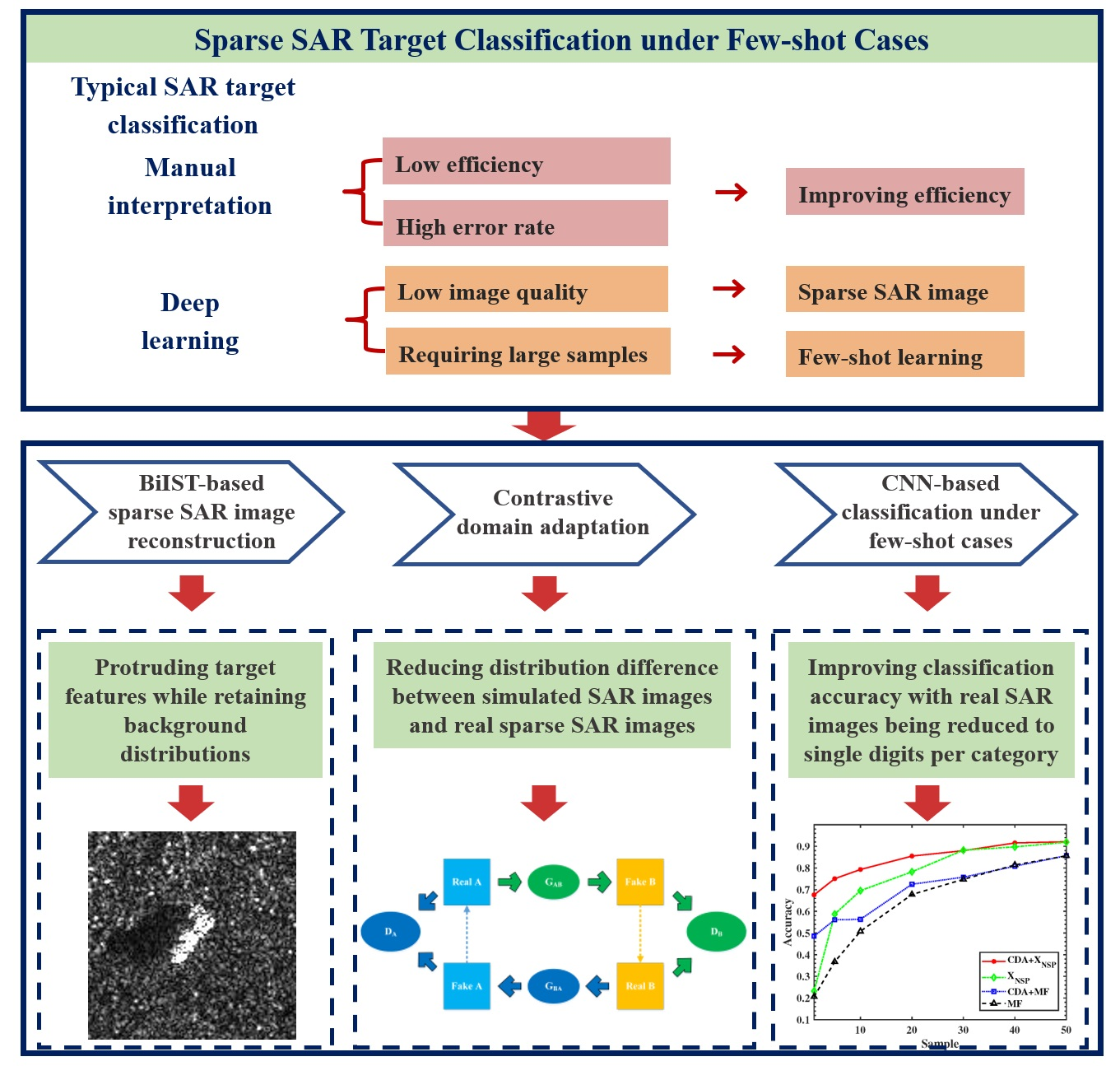
In this paper, we propose a novel sparse SAR target classification method based on contrastive domain adaptation (CDA) for a few shots. In the proposed method, we firstly use the BiIST algorithm to improve the MF-based SAR image performance, and hence construct a novel sparse SAR dataset. Then, the simulated dataset and constructed sparse dataset are sent into an unsupervised domain adaptation framework, so as to transfer target features and minimize distribution difference. After the CDA operation, the reconstructed simulated SAR image which has a similar background distribution and target features to real SAR image will be manually labeled for subsequent classification. Finally, the reconstructed simulated SAR image will be trained in a shallow CNN along with a few real samples. Experimental results based on the MSTAR dataset under standard operating conditions (SOC) show that compared to several typical deep learning methods for SAR target classification, the proposed method presents similar or better performance with enough real samples. With the decrease of the number of real SAR images, the proposed method achieves higher accuracy than other methods, showing great potential for application in real scenes under the extreme shortage of labeled real images.
The main contributions of this paper can be concluded as follows. 1. This paper first applies an unsupervised contrastive domain adaptation framework to minimize the distribution difference between a simulated SAR dataset and real sparse SAR images so as to facilitate transfer learning in sparse SAR image classification. 2. In view of the serious shortage of labeled SAR images in practical applications, the proposed method improves classification accuracy with the real sparse SAR images being reduced to single digits per class.
The rest of this paper is organized as follows. Section 2 introduces the procedure of constructing a sparse real dataset by the BiIST algorithm and the principle of the common transfer learning method. The key process of the proposed algorithm, i.e., CDA, is discussed in Section 3, including components of the unsupervised domain adaptation framework and theories of minimizing the distribution difference between the two datasets. The model of CNN used for target classification is described in Section 4. Experiments based on the sparse MSTAR dataset and the reconstructed simulated dataset under different conditions are shown in Section 5. Section 6 analyzes the experimental results in detail. At last, Section 7 concludes this work.
2. Methodology
2.1. BiIST-Based Sparse SAR Dataset Construction
Although the SAR image recovered by the MF algorithm is more convenient to obtain, it has serious noise with ambiguous target features, which affects its further application in target classification. Therefore, we want to obtain higher-quality images to support subsequent applications. Using the MF-based image as input, the sparse SAR imaging model based on complex image data can be expressed as [22,23]
where is the backscattering coefficient of the interested area to be recovered, represents the difference between and . Then, we can reconstruct by solving
where is the regularization parameter and subscript F denotes the Frobenius norm. As demonstrated in [22,23], BiIST is able to output two kinds of sparse SAR images called sparse solution () and non-sparse solution (). Similar to OMP and IST, improves the image quality with less noise but damages the background distribution and phase information. Compared with , not only obtains improved SAR image while remaining the background distribution, offering more information for subsequent CDA and target classification. In the following, the real sparse SAR image refers to recovered by BiIST.
2.2. Transfer Learning
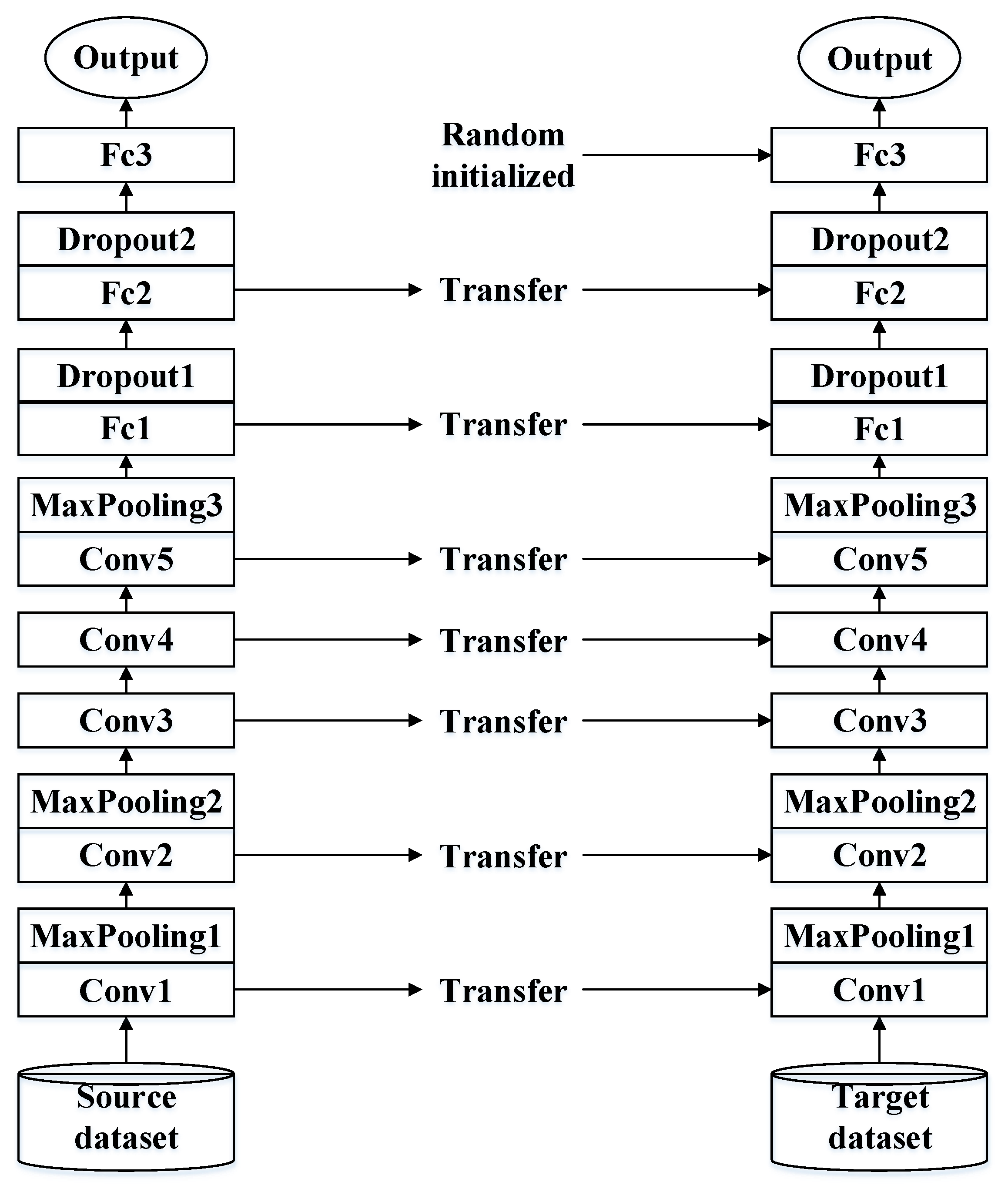
The idea of transfer learning (TL) in the field of computer vision (CV) aims to imitate human learning behavior. Firstly, the deep learning frameworks are pretrained on large amounts of data to learn the general features, then these frameworks are applied to specific tasks to reduce calculation and improve performance. Benefiting from the abundant optical image datasets, transfer learning is widely used in practical applications. The traditional transfer learning method is shown in Figure 1. It can be seen that after pretraining the framework with abundant data in source domain, only the last fully connected layer is randomly initialized while parameters in the rest of the framework are fixed. The number of classes in the dataset used for pretraining the network is then changed to the number of classes in the target dataset. However, this method fails to operate in SAR image classification and can be explained from two aspects. Firstly, different from abundant optical image datasets, the lack of labeled SAR image datasets cannot afford the pretraining of the network. In addition, between A and B due to the imaging mechanism of SAR, the same kind of target under different imaging modes or imaging parameters will be different, which may hinder the development of transfer learning in the field of SAR image processing.
Therefore, in this paper, we take above problems into consideration and propose a novel transfer learning method used for sparse SAR target classification, i.e., the contrastive domain adaptation-based sparse SAR target classification. In the proposed method, the training process is a two-step procedure. Firstly, a simulated SAR dataset and real SAR data are simultaneously sent into an unsupervised domain adaptation framework to reduce the distribution difference and obtain the reconstructed simulated SAR images for subsequent target classification. Secondly, the reconstructed simulated images and a few real sparse SAR images form the input of CNN for further target classification.
3. Feature Learning-Based Contrastive Domain Adaptation
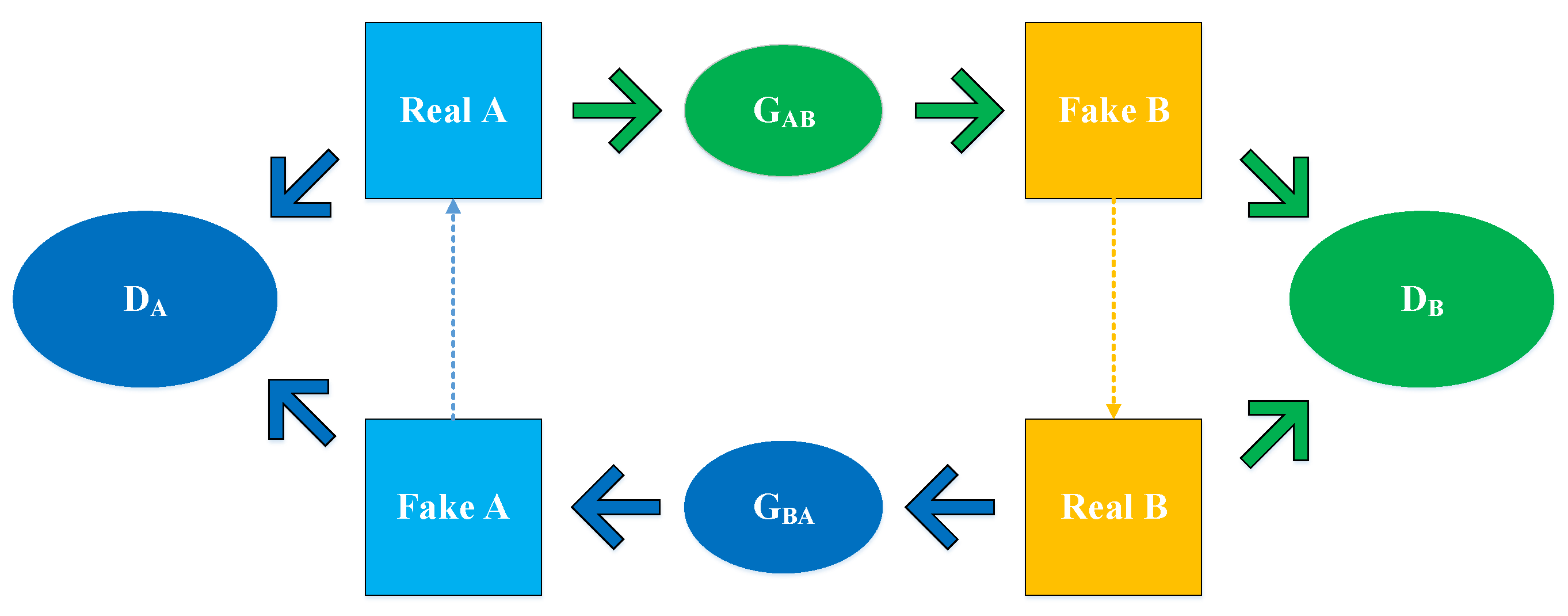
The key process of the proposed method is described in detail in this section. The flowchart of the unsupervised domain adaptation framework is shown in Figure 2, whose input consists of the simulated SAR dataset and dataset . Two image reconstruction models and two discrimination models form a closed loop so as to make the simulated SAR dataset and dataset learn characteristics from each other. In Figure 3, the image reconstruction model represents the transition from to . is the opposite, which has the same structure as . Discrimination model is used to identify whether the input data are a reconstructed simulated SAR target or a real sparse SAR target, and shows the opposite. Similarly, and have the same structure as well. The principles of CDA will be explained in the following.
3.1. Feature Learning
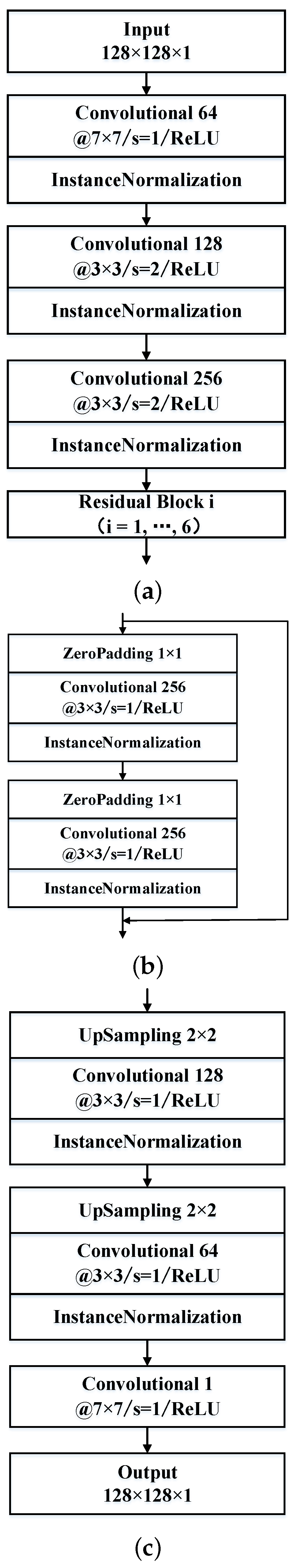
Take the transition from the simulated SAR dataset to the dataset as an example. Firstly, goes through to generate an image which has a similar distribution to . The architecture of is made up of two modules, i.e., feature extraction module and feature restoration module, as shown in Figure 3. The feature extraction module is depicted in Figure 3a,b. It firstly uses several convolutional layers to extract target features and reduce the dimension of the feature map to . Six residual blocks are then followed after the convolutional layer to deepen the network. It should be noted that the residual block is only used to learn the target features and does not change the size of the feature map to facilitate the subsequent feature restoration.
3.2. Feature Restoration
The feature restoration module is shown in Figure 3c, which forms the second part of the image reconstruction model. It is found that through multiple up-sampling layers and convolutional layers, the final output is an image of size , i.e., the same as the input simulated image. The output feature map of up-sampling layer can be written as
where , , denote the height, width, and number of channels of the output feature map. Similarly, , , represent those of the input feature map. f is the kernel size of the up-sampling layer and is set to 2 in this paper. Moreover, it should be noted that the number of channels of the convolutional layer in the feature restoration module corresponds to the one in the feature extraction module, e.g., the channels of the first convolutional layer in the feature restoration module are the same as those of the second convolutional layer in the feature extraction module to keep the same number of the feature map.
3.3. Image Discrimination
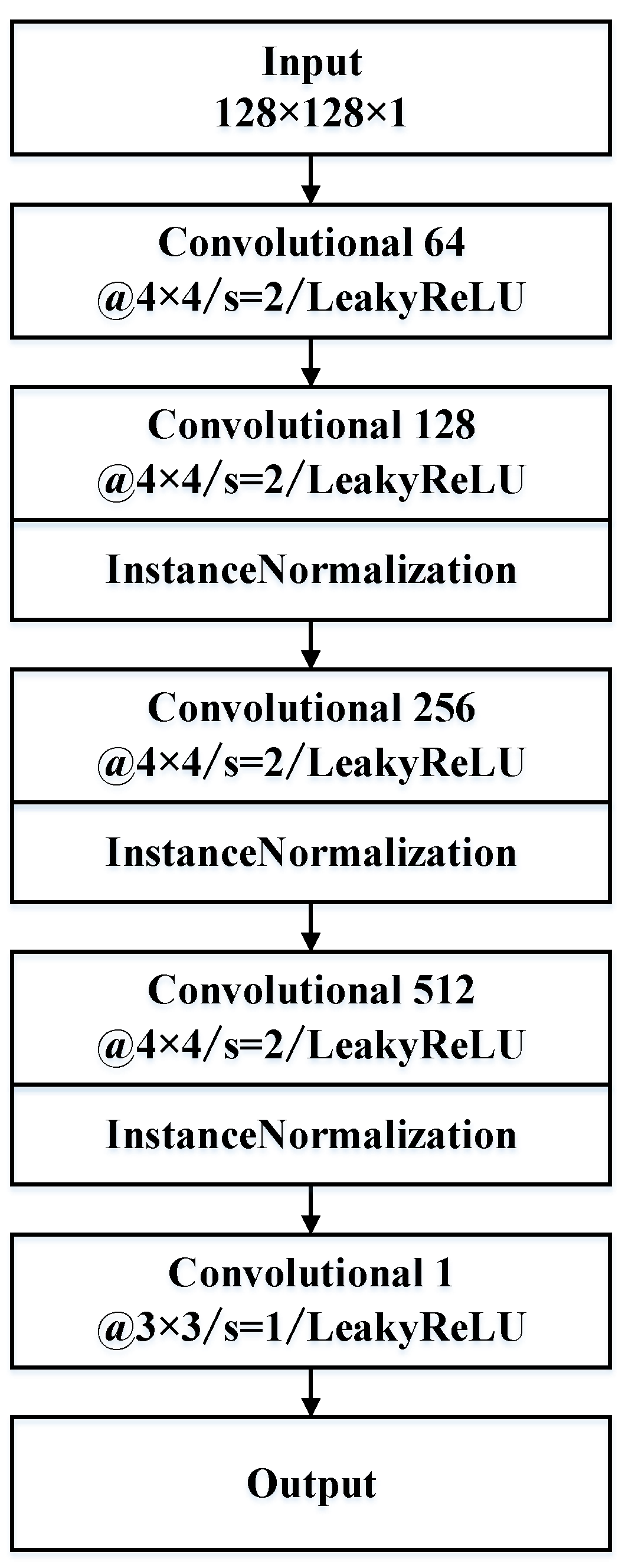
Then, a discrimination model is used to identify whether the input data are the reconstructed simulated SAR image or sparse real SAR image, whose structure is shown in Figure 4. In order to maximize the potential of the discriminant model, all the information in each pixel of the input image should be considered and used. Therefore, an activation function named Leaky ReLU is adopted in each convolutional layer, which can be defined as
where denotes the value in the pixel of i-th row and j-th column, is a constant which is set to 0.2 in this paper to retain negative values and avoid the loss of information in the negative axis. It should be noted that instance normalization (IN) is used after each convolutional layer, whether it is an image reconstruction model or a discriminative model. Different from batch normalization (BN) that processes elements of all images in a batch, IN only focuses on the elements of an image so that it can maintain the unique characteristics of each sample. After four convolution operations, the last convolution layer reduces the dimension of the feature map to , i.e., 64 pixels. The output value of each pixel is zero or one. Zero means that the input data are a reconstructed simulated SAR image generated through the above network. One represents that the input is a real sparse SAR target. The final result is obtained by comprehensive evaluation of 64 output values. During the discrimination process, mean squared error (MSE) is used to measure the difference between reconstructed simulated image and , defined as
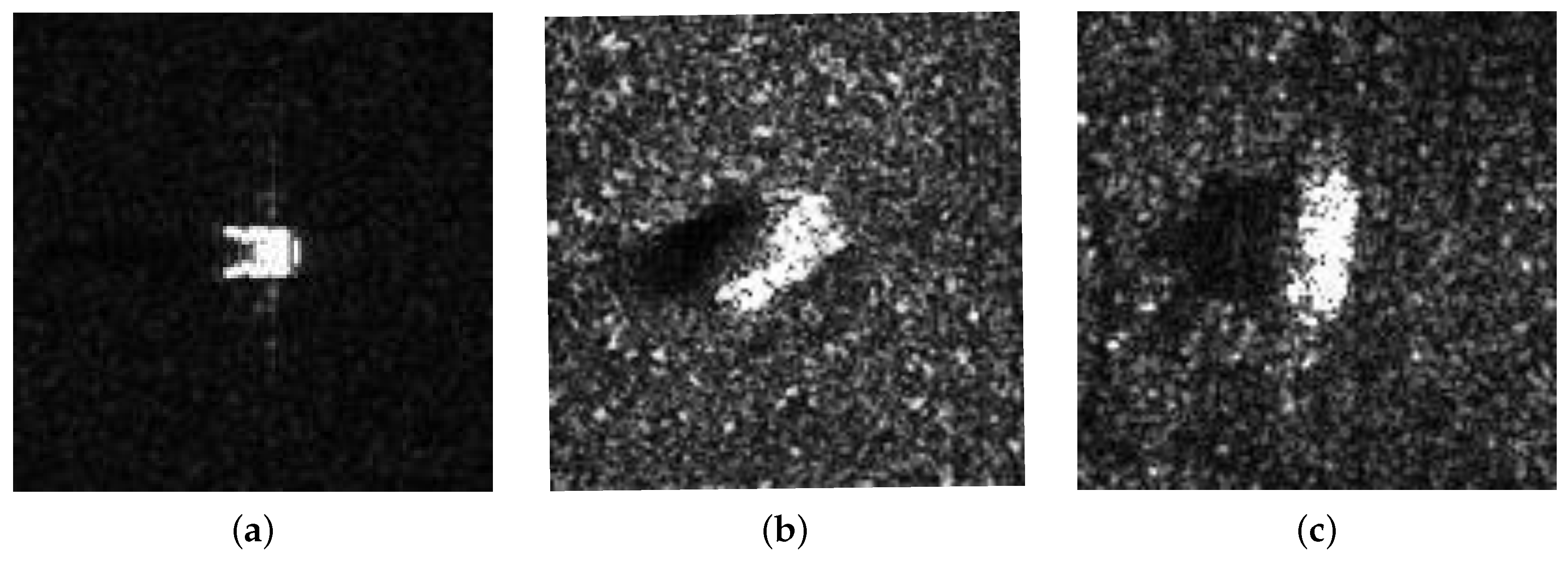
where denotes the number of images in the dataset , is the n-th sample of , and is the corresponding reconstructed sample. After multiple epochs of iterative training, the model is able to generate an image that is closer to (see Figure 5).
Since the two networks used to generate images have the same structure, the simulated SAR images and the sparse SAR images are not paired, i.e., the number of samples in the two datasets is different. In order to ensure that the input samples of each epoch learn the correct mapping from each other during the training process, a constraint condition is added into the framework, which is defined as
where indicates the simulated image, generates an image through and then restores it by , is used to tell the difference between the restored image and the original . Similarly, indicates the simulated image, generates an image through and then restores it by while measures the difference between the restored image and the original . will also learn to simulate the target features of the simulated SAR image through the model and , thereby accelerating the reduction of the distribution between and . The principle of transition from to is the same as that described above.
4. CNN-Based Sparse SAR Target Classification
4.1. Principle
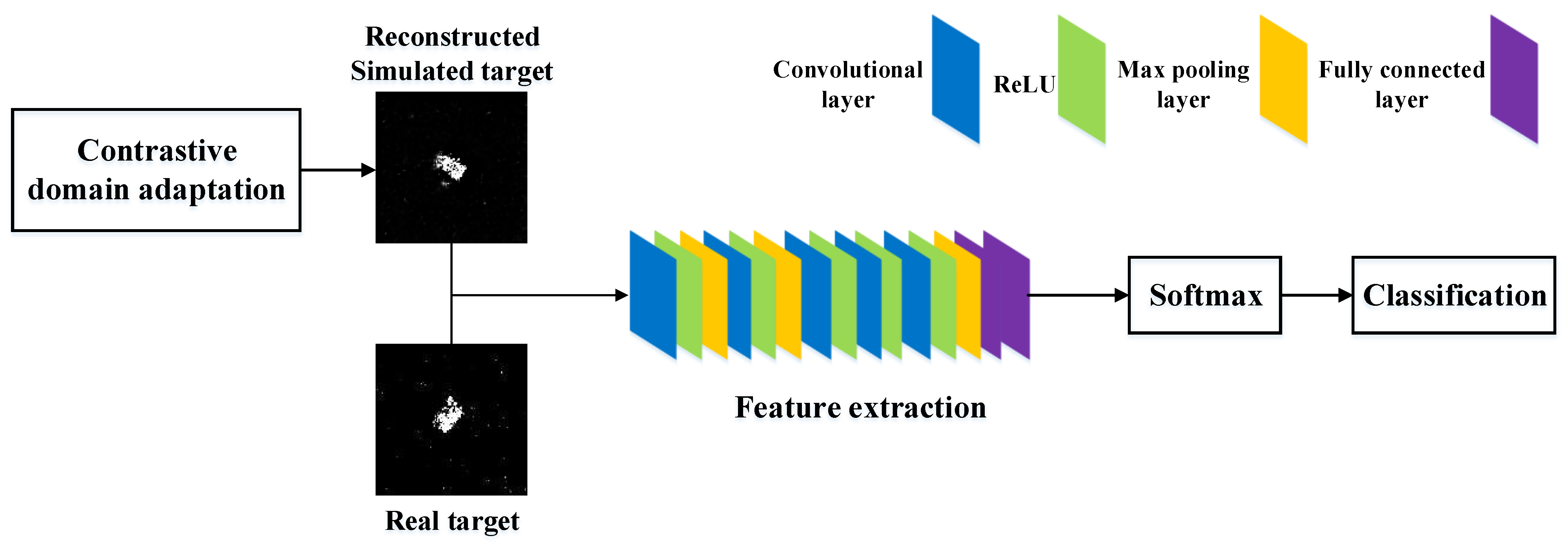
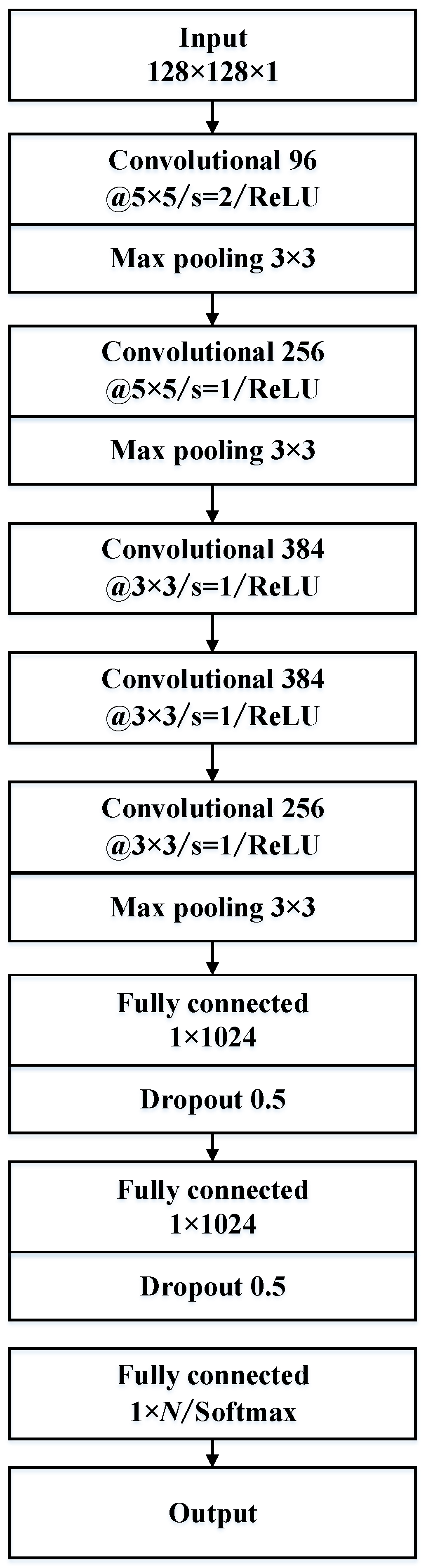
Due to the advantages of weight sharing and local connections, CNN has a strong ability in extracting target features without increasing the complexity of the target classification framework. Therefore, in this section, a shallow CNN model is used to classify the sparse SAR target after acquiring a large number of reconstructed simulated SAR images. The flowchart of the SAR target classification is shown in Figure 6. After contrastive domain adaptation, we acquire abundant reconstructed simulated targets which have similar distributions to real SAR images. It is found that the reconstructed simulated SAR images and few real SAR images form the input of CNN and go through multiple convolutional layers and max pooling layers to extract target features. Finally, the softmax activation function is chosen to classify targets. The detailed components of the classification model are presented in Figure 7. As shown in Figure 7, the feature extraction framework consists of five convolutional layers, three max pooling layers, and two fully connected layers. The convolutional layer is different from the traditional neural network. It contains several convolution kernels to extract image characteristics one by one, greatly reducing the parameters in the network. This calculation is described as
where k means that the size of the kernel is , is the weight of i-th row and j-th column in the kernel, represents the value of i-th row and j-th column in the region covered by the convolution kernel, denotes the element of i-th row and j-th column in the output feature map, and b means bias which is set to 0 in many cases so as to reduce the computational complexity. The max pooling layer reduces the dimension of the feature map to further decrease the calculation. The size of the output feature map is
where s determines stride, and m shows the size of the pooling box. The fully connected layer is responsible for integrating the extracted features and preparing them for classification. To alleviate the overfitting problem caused by limited real targets, two dropout layers are placed after the fully connected layer to randomly prevent some neurons from participating in the training of each epoch and to improve the robustness of the classification framework.
4.2. Training Details
During the training process, the learning rate and epoch are set to 0.0005 and 200, respectively. The input dataset is usually separated into training set, validation set, and testing set. The training set is responsible for updating parameters in the network. The validation set separated from the training set is used to monitor the network training. While the testing set does not join the training process and is utilized to evaluate the robustness of the model. It is noted that in this paper, the reconstructed simulated data and a few sparse SAR images form the training set, but the validation set only consists of real SAR data in the training set. Each category in the training set is made up of 190 reconstructed simulated images and a few real sparse SAR images ranging from 1 to 50.
5. Experimental Results Based on MSTAR Dataset
In this section, we take MSTAR as our basic dataset, which is commonly used in SAR image classification. In order to validate the proposed method, we divide the experiments into three main parts. First, experiments under four different situations are conducted to validate whether CDA promotes the classification performance when real samples are insufficient. In the second part of experiments, several typical deep learning methods are used to compare with the proposed method. Finally, experiments under EOC are carried out in which characteristics in the training set and testing set differ a lot, bringing great difficulty for SAR target classification.
5.1. Dataset
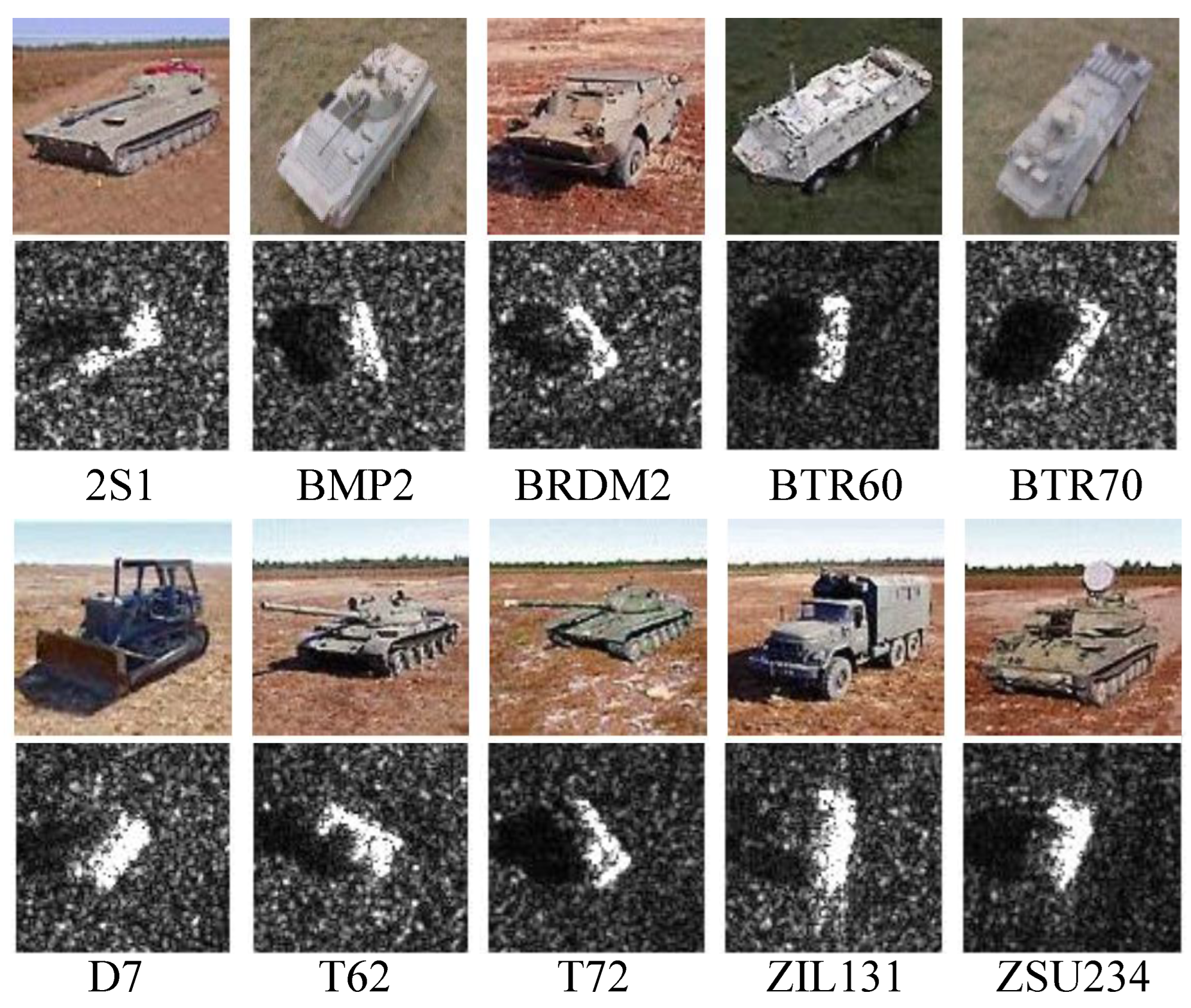
In the experiments, the dataset is constructed based on MSTAR. MSTAR is a MF-based dataset including 10 kinds of military vehicles. The detailed data description of MSTAR under SOC is shown in Table 1, including serial number, number of samples in the training set and testing set. Data in MSTAR are collected at two depression angles ranging from to azimuth angle. All the experiments are conducted under SOC. The samples of are for the training set, while the images of become the testing set. The optical images and corresponding SAR images of the ten category vehicles are shown in Figure 8. In the experiments, we suppose that only few labeled real sparse SAR images are available, so the samples at are randomly selected to be 1, 5, 10, 20, 30, 40, and 50 per class.
5.2. Study Based on Different Input Data
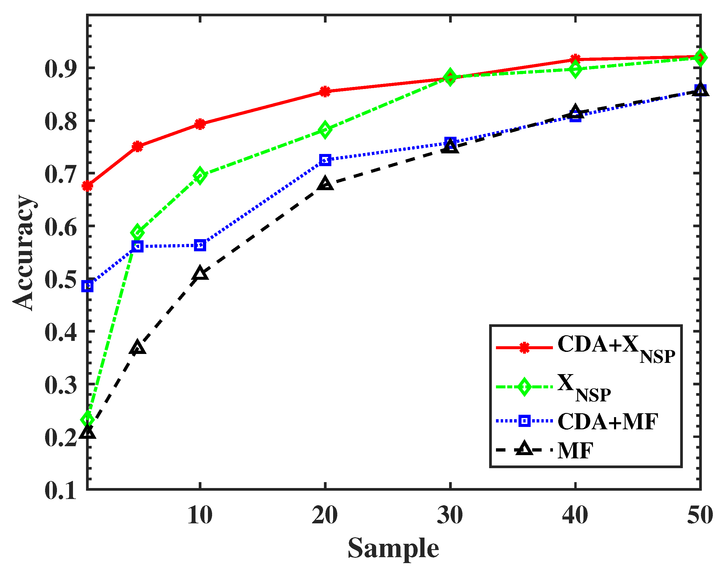
In order to support our viewpoints, the experiments based on both MF-recovered dataset and sparse SAR dataset are carried out simultaneously. As shown in Figure 9, experimental results of different numbers of training samples under four situations are taken into consideration. It can be concluded from two aspects that without CDA, CNN reaches similar accuracy when training data are sufficient, but fails to present similar performance with training samples decreasing. In addition, compared with the MF-based dataset, the dataset achieves higher classification accuracy no matter the number of training samples. Take 5 samples of each class as example, the combination of CDA and sparse SAR dataset outperforms others by 20.6%, 28.0%, and 38.3%, respectively. The confusion matrix in Table 2 shows the classification result of the combination of CDA and sparse dataset, including both correctly and misclassified targets. It is seen that when only 20 training samples per class are available, the accuracy rate can reach more than 80%, and even targets such as T62 and ZSU234 can achieve more than 95%.
5.3. Comparison between Different Methods
To further validate the proposed method, several deep learning methods used for SAR target classification via few shots are adopted to be comparative experiments. As shown in Table 3, it can be seen that the proposed method achieves higher classification accuracy than CHU and A-ConvNet under all sets of training samples. In addition, when real SAR images are sufficient, the accuracy of M-Net is close to the proposed method. However, when it comes to the small sample case, i.e., with less than 30 samples per class, the proposed method shows better classification performance. While when the number of real SAR images decreases to 20 samples per class, the proposed method achieved 85.5% classification accuracy, respectively outperforming CHU, A-ConvNet, and M-Net by 44.5%, 19.5%, and 8.8%. Moreover, it should be noted that even if only 5 samples per class are available, our method can still achieve more than 75% accuracy. The performance gap with other methods is even more obvious.
5.4. Verification under EOC
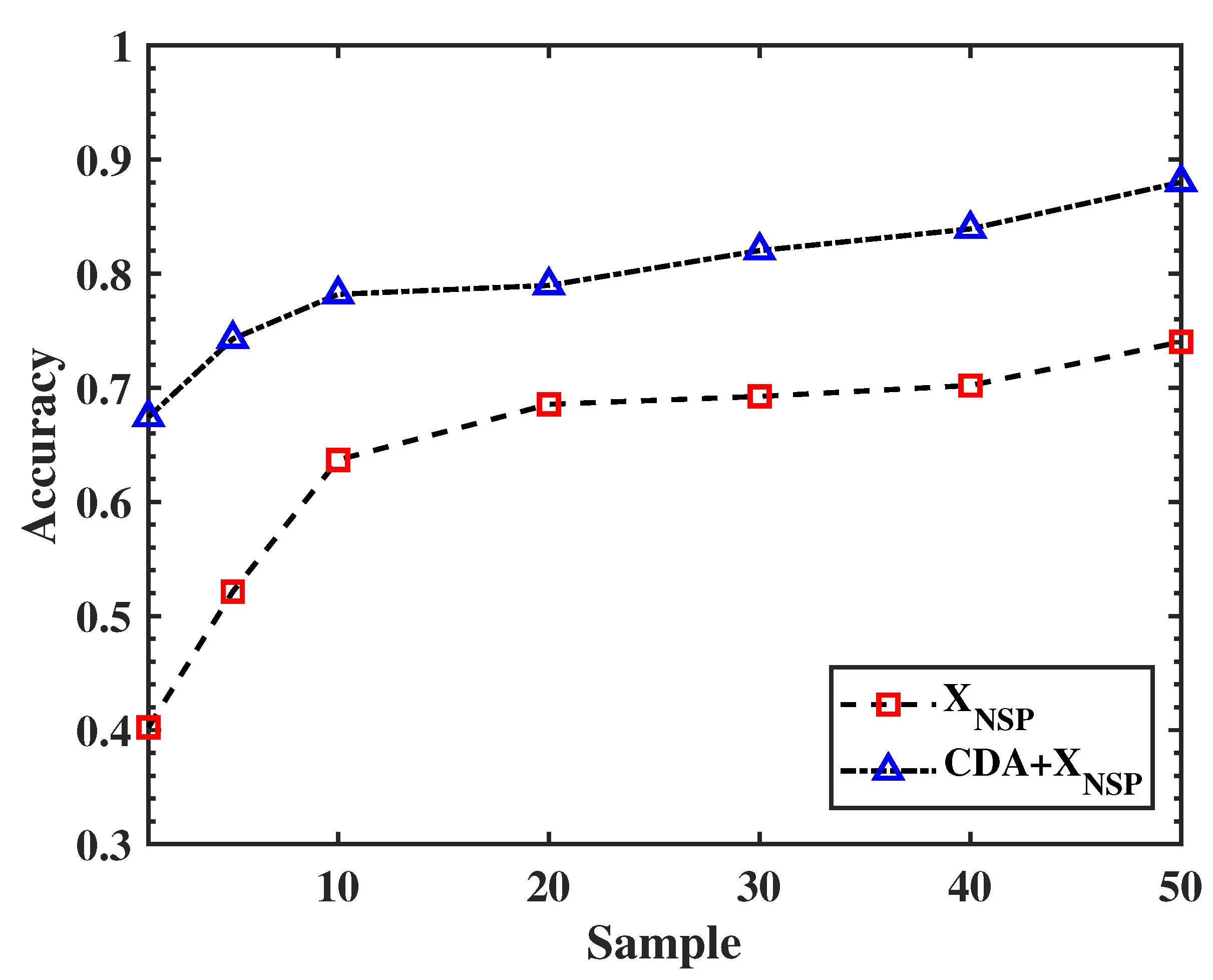
Considering the generalization of the proposed method, experiments under EOC are carried out as well, in which samples in the training set and testing set differ a lot. Data description for EOC is shown in Table 4, including each category’s serial number and number of samples. It can be seen that some military vehicles have different types in the training set and testing set, e.g., the type of T72 in the training set is SN132, but A64 in the testing set, which brings more difficulty for SAR target classification. Experimental results demonstrate the combination of the dataset and CDA achieves better performance than the dataset only, as shown in Figure 10. With real samples decreasing, the performance gap becomes more obvious. Table 5 presents the confusion matrix of classification accuracy based on CDA and the sparse SAR image via 5 samples per class, in which the misclassified targets and targets being correctly classified are recorded in detail. As shown in the table, although ZSU234 reaches a relatively low accuracy of 40.97%, targets such as T72 and BRDM2 achieve around 80% accuracy with only 5 real SAR targets, even 2S1 still achieves over 90% classification accuracy. In Table 6, more indicators are selected to evaluate the experiments. The precision rate denotes the correct proportion of model predictions in all predicted samples. The recall rate is close to classification accuracy which means that the proportion of samples is correctly predicted to all the real samples. F1-score which is written as represents a comprehensive evaluation of precision and recall. Table 5 and Table 6 give a comprehensive evaluation of experimental results via 5 samples per class.
In this section, several experiments on the basis of the MF-based dataset and BiIST-based dataset are conducted to validate the proposed method. From the above analysis, it can be concluded that the CDA-based sparse SAR target classification method can improve the performance or achieve optimal accuracy in the comparison with others under each set of training samples, especially under few-shot cases.
6. Experimental Analysis
Experimental results on SAR target classification can mainly be divided into two scenarios. Under SOC, we carry out four comparative experiments under different sets of training samples ranging from 1 per class to 50 per class. On the one hand, the combination of and CDA achieves similar performance to when the real samples are sufficient, but outperforms with real sparse SAR images reducing. On the other hand, no matter the number of training data, the combination of and CDA always reaches higher classification accuracy compared with MF and the combination of CDA and MF, showing the great potential of non-sparse SAR images. Under EOC, targets in training set and testing set differ a lot; hence, it can be found that CDA is able to improve classification performance especially in the situation of fewer training samples. When the number of training samples comes to 5 per category, the combination of and CDA can still reach over 70% accuracy, which shows the great potential of applying the proposed method in real scenes.
7. Conclusions
In this paper, a novel sparse SAR target classification method on the basis of CDA is proposed for few-shot cases. Experimental results show that compared to typical classification methods via small samples, the proposed method has similar accuracy when there are sufficient real SAR samples. However, with the used real SAR images decreasing to 5 or 10 samples of each category, the accuracy gap between the proposed method and others is more obvious. In addition, it should be also noted that the combination of and CDA obtains optimal performance under SOC and EOC, proving the efficiency and generalization in SAR applications. To further reduce real SAR images while improving the accuracy, we will explore how to integrate phase information in the future.
Author Contributions
Conceptualization, H.B. and J.Z.; methodology, Z.L., J.D. and Z.J.; validation, Z.L. and J.D.; writing—original draft preparation, Z.L. and J.D.; writing—review and editing, Z.J., H.B. and J.Z. All authors have read and agreed to the published version of the manuscript.
Funding
This work was supported in part by the National Natural Science Foundation of China under Grant 62271248 and 61901213, in part by Guangdong Basic and Applied Basic Research Foundation under Grant 2020B1515120060, in part by the Aeronautical Science Foundation of China under Grant 201920052001, and in part by the University Joint Innovation Fund Project of CALT under Grant CALT2021-11.
Data Availability Statement
The complex SAR image data used in this paper is the MSTAR dataset, which can be found at https://www.sdms.afrl.af.mil/index.php?collection=mstar (accessed on 3 August 2022).
Conflicts of Interest
The authors declare no conflict of interest.
Abbreviations
The following abbreviations are used in this paper:
| DA | Domain Adaptation |
| CDA | Contrastive Domain Adaptation |
| HDA | Heterogeneous Domain Adaptation |
| SAR | Synthetic Aperture Radar |
| CV | Computer Vision |
| MF | Matched Filtering |
| ATR | Automatic Target Recognition |
| CHU | Convolutional Highway Unit |
| A-ConvNets | All-convolutional Networks |
| CV-CNN | Complex-valued Convolutional Neural Network |
| CV-FCNN | Complex-valued Fully Convolutional Neural Network |
| IST | Iterative Soft Thresholding |
| OMP | Orthogonal Matching Pursuit |
| CNN | Convolutional Neural Network |
| ReLU | Rectified Linear Unit |
| CReLU | Concatenated Rectified Linear Unit |
| DL | Deep Learning |
| TL | Transfer Learning |
| GAN | Generative Adversarial Network |
| MD-GAN | Multi-discriminators Generative Adversarial Network |
| CAE | Convolutional Autoencoder |
| CCAE | Compact Convolutional Autoencoder |
| DJ-CORAL | Dynamic Joint Correlation Alignment Network |
| Fc | Fully Connected Layer |
| RCNN | Regional Convolutional Neural Network |
| YOLO | You Only Look Once |
| AP-CNN | Amplitude-phase Convolutional Neural Network |
| IN | Instance Normalization |
| BN | Batch Normalization |
| MSE | Mean Squared Error |
| MSTAR | Moving and Stationary Target Acquisition and Recognition |
| SOC | Standard Operating Conditions |
| EOC | Extended Operating Conditions |
References
- Curlander, J.C.; Mcdonough, R.N. Synthetic Aperture Radar: Systems and Signal Processing; Wiley: New York, NY, USA, 1991. [Google Scholar]
- Henderson, F.M.; Lewis, A.J. Principle and Application of Imaging Radar; John Wiley and Sons: New York, NY, USA, 1998. [Google Scholar]
- Dugeon, D.E.; Lacoss, R.T. An overview of automatic target recognition. Linc. Lab. J. 1993, 6, 3–10. [Google Scholar]
- Kreithen, D.E.; Halversen, S.D.; Owirka, G.J. Discriminating targets from clutter. Linc. Lab. J. 1993, 6, 25–51. [Google Scholar]
- Hinton, G.E.; Salakhutdinov, R.R. Reducing the dimensionality of data with neural networks. Science 2006, 313, 504–507. [Google Scholar] [CrossRef] [PubMed] [Green Version]
- Krizhevsky, A.; Sutskever, I.; Hinton, G.E. Imagenet classification with deep convolutional neural networks. Commun. ACM 2012, 60, 84–90. [Google Scholar] [CrossRef] [Green Version]
- Russakovsky, O.; Deng, J.; Su, H.; Krause, J.; Satheesh, S.; Ma, S.; Huang, Z.; Karpathy, A.; Khosla, A.; Bernstein, M.; et al. Imagenet large scale visual recognition challenge. Int. J. Comput. Vis. 2015, 115, 211–252. [Google Scholar] [CrossRef] [Green Version]
- Szegedy, C.; Liu, W.; Jia, Y.; Sermanet, P.; Reed, S.; Anguelov, D.; Erhan, D.; Vanhoucke, D.; Rabinovich, A. Going deeper with convolutions. In Proceedings of the 2015 IEEE Conference on Computer Vision and Pattern Recognition (CVPR), Boston, MA, USA, 7–12 June 2015. [Google Scholar]
- He, K.; Zhang, X.; Ren, S.; Sun, J. Delving deep into rectifiers: Surpassing human-level performance on ImageNet classification. In Proceedings of the 2016 IEEE Conference on Computer Vision and Pattern Recognition (CVPR), Santiago, Chile, 26 June–1 July 2016. [Google Scholar]
- Huang, G.; Liu, Z.; der Maaten, L.; Weinberger, K.Q. Densely connected convolutional networks. In Proceedings of the 2017 IEEE Conference on Computer Vision and Pattern Recognition (CVPR), Honolulu, HI, USA, 21–26 July 2017. [Google Scholar]
- Ding, J.; Chen, B.; Liu, H.; Huang, M. Convolutional neural network with data augmentation for SAR target recognition. IEEE Geosci. Remote Sens. Lett. 2016, 13, 364–368. [Google Scholar] [CrossRef]
- Chen, S.; Wang, H.; Xu, F.; Qiu, Y. Target classification using the deep convolutional networks for SAR images. IEEE Trans. Geosci. Remote Sens. 2016, 54, 4806–4817. [Google Scholar] [CrossRef]
- Hansen, D.M.; Kusk, A.; Dall, J.; Nielsen, A.A.; Engholm, R.; Skriver, H. Improving SAR automatic target recognition models with transfer learning from simulated data. IEEE Geosci. Remote Sens. Lett. 2017, 14, 1484–1488. [Google Scholar] [CrossRef] [Green Version]
- Lin, Z.; Ji, K.; Kang, M.; Leng, X.; Zou, H. Deep convolutional highway unit network for SAR target classification with limited labeled training data. IEEE Geosci. Remote Sens. Lett. 2017, 14, 1091–1095. [Google Scholar] [CrossRef]
- Zhong, C.; Mu, X.; He, X.; Wang, J.; Zhu, M. SAR target image classification based on transfer learning and model compression. IEEE Geosci. Remote Sens. Lett. 2019, 16, 412–416. [Google Scholar] [CrossRef]
- Wang, Z.; Xu, X. Efficient deep convolutional neural networks using CReLU for ATR with limited SAR images. J. Eng. 2019, 2019, 7615–7618. [Google Scholar] [CrossRef]
- Zhang, W.; Zhu, Y.; Fu, Q. Deep transfer learning based on generative adversarial networks for SAR target recognition with label limitation. In Proceedings of the 2019 IEEE International Conference on Signal, Information and Data Processing (ICSIDP), Chongqing, China, 11–13 December 2019. [Google Scholar]
- Zheng, C.; Jiang, X.; Liu, X. Semi-Supervised SAR ATR via multi-discriminator generative adversarial network. IEEE Sens. J. 2019, 19, 7525–7533. [Google Scholar] [CrossRef]
- Guo, J.; Wang, L.; Zhu, D.; Hum, C. Compact convolutional autoencoder for SAR target recognition. IET Radar Sonar Navig. 2020, 14, 967–972. [Google Scholar] [CrossRef]
- Huang, Z.; Pan, Z.; Lei, B. What, where, and how to transfer in SAR target recognition based on deep CNNs. IEEE Trans. Geosci. Remote Sens. 2020, 58, 2324–2336. [Google Scholar] [CrossRef] [Green Version]
- Guo, Y.; Du, L.; Lyu, G. SAR target detection based on domain adaptive Faster R-CNN with small training data size. Remote Sens. 2021, 13, 4202. [Google Scholar] [CrossRef]
- Yang, G.; Lang, H. Semisupervised heterogeneous domain adaptation via dynamic joint correlation alignment network for ship classification in SAR imagery. IEEE Geosci. Remote Sens. Lett. 2022, 19, 1–5. [Google Scholar] [CrossRef]
- Zhang, Z.; Wang, H.; Xu, F.; Jin, Y.-Q. Complex-valued convolutional neural network and its application in polarimetric SAR image classification. IEEE Trans. Geosci. Remote Sens. 2017, 55, 7177–7188. [Google Scholar] [CrossRef]
- Coman, C.; Thaens, R. A deep learning SAR target classification experiment on MSTAR dataset. In Proceedings of the 19th International Radar Symposium (IRS), Bonn, Germany, 20–22 June 2018. [Google Scholar]
- Yu, L.; Hu, Y.; Xie, X.; Lin, Y.; Hong, W. Complex-valued full convolutional neural network for SAR target classification. IEEE Geosci. Remote Sens. Lett. 2020, 17, 1752–1756. [Google Scholar] [CrossRef]
- Daubechies, I.; Defriese, M.; De Mol, C. An iterative thresholding algorithm for linear inverse problems with a sparsity constraint. Commun. Pure Appl. Math. 2004, 57, 1413–1457. [Google Scholar] [CrossRef] [Green Version]
- Bi, H.; Bi, G. Performance analysis of iterative soft thresholding algorithm for L1 regularization based sparse SAR imaging. In Proceedings of the 2019 Radar Conference (RadarConf), Boston, MA, USA, 22–26 April 2019. [Google Scholar]
- Pati, Y.C.; Rezaiifar, R.; Krishnaprasad, P.S. Orthogonal matching pursuit: Recursive function approximation with applications to wavelet decomposition. In Proceedings of the 27th Asilomar Conference on Signals, Systems and Computers, Pacific Grove, CA, USA, 1–3 November 1993. [Google Scholar]
- Donoho, D.L.; Tsaig, Y.; Drori, I.; Starck, J. Sparse solution of underdetermined systems of linear equations by stagewise orthogonal matching pursuit. IEEE Trans. Inf. Theory 2012, 58, 1094–1121. [Google Scholar] [CrossRef]
- Bi, H.; Bi, G.; Zhang, B.; Hong, W. A novel iterative thresholding algorithm for complex image based sparse SAR imaging. In Proceedings of the 12th European Conference on Synthetic Aperture Radar (EUSAR), Aachen, Germany, 4–7 June 2018. [Google Scholar]
- Bi, H.; Bi, G. A novel iterative soft thresholding algorithm for L1 regularization based SAR image enhancement. Sci. China Inf. Sci. 2019, 62, 49303. [Google Scholar] [CrossRef] [Green Version]
- Bi, H.; Deng, J.; Yang, T.; Wang, J.; Wang, L. CNN-based target detection and classification when sparse SAR image dataset is available. IEEE J. Sel. Top. Appl. Earth Obs. Remote Sens. 2021, 14, 6815–6826. [Google Scholar] [CrossRef]
- Deng, J.; Bi, H.; Zhang, J.; Liu, Z.; Yu, L. Amplitude-phase CNN-based SAR target classification via complex-calued sparse image. IEEE J. Sel. Top. Appl. Earth Obs. Remote Sens. 2022, 15, 5214–5221. [Google Scholar] [CrossRef]
- Shang, R.; Wang, J.; Jiao, L.; Stolkin, R.; Hou, B.; Li, Y. SAR targets classification based on deep memory convolution neural networks and transfer parameters. IEEE J. Sel. Top. Appl. Earth Obs. Remote Sens. 2018, 11, 2834–2846. [Google Scholar] [CrossRef]
Figure 1.
Details of the traditional transfer learning method.

Figure 2.
Overview of the contrastive domain adaptation.

Figure 3.
Architecture of the image reconstruction model. (a) Feature extraction module. (b) Details of the residual block. (c) Feature restoration module.
Figure 3.
Architecture of the image reconstruction model. (a) Feature extraction module. (b) Details of the residual block. (c) Feature restoration module.

Figure 4.
Structure of the discrimination model.

Figure 5.
Presentation of three kinds of SAR images. (a) Original simulated SAR image. (b) Reconstructed simulated SAR image. (c) .
Figure 5.
Presentation of three kinds of SAR images. (a) Original simulated SAR image. (b) Reconstructed simulated SAR image. (c) .

Figure 6.
Flowchart of the target classification.

Figure 7.
Structure of the classification framework.

Figure 8.
Optical images and corresponding SAR images of vehicles in the MSTAR dataset.

Figure 9.
Experimental results of different training samples based on MF-based image and sparse image under SOC.
Figure 9.
Experimental results of different training samples based on MF-based image and sparse image under SOC.

Figure 10.
Experimental results of different training samples based on sparse image under EOC.


Table 1.
Data description for SOC.
| Class | Serial No. | Training Set (Depression 17°) | Testing Set (Depression 15°) |
|---|---|---|---|
| 2S1 | B01 | 299 | 274 |
| BMP2 | SN9563 | 233 | 196 |
| BRDM2 | E-71 | 298 | 274 |
| BTR60 | Kloyt7532 | 256 | 195 |
| BTR70 | C71 | 233 | 196 |
| D7 | 92v13015 | 299 | 274 |
| T62 | A51 | 299 | 273 |
| T72 | SN132 | 232 | 196 |
| ZIL131 | E12 | 299 | 274 |
| ZSU234 | D08 | 299 | 274 |
| Total | 2747 | 2426 |
Table 2.
Confusion matrix of classification accuracy based on the CDA and sparse SAR image via 20 samples per class.
Table 2.
Confusion matrix of classification accuracy based on the CDA and sparse SAR image via 20 samples per class.
| Class | 2S1 | BMP2 | BRDM2 | BTR60 | BTR70 | D7 | T62 | T72 | ZIL131 | ZSU234 | Total |
|---|---|---|---|---|---|---|---|---|---|---|---|
| 2S1 | 218 | 2 | 4 | 19 | 5 | 2 | 12 | 9 | 2 | 1 | |
| BMP2 | 14 | 108 | 4 | 15 | 35 | 0 | 2 | 16 | 0 | 2 | |
| BRDM2 | 0 | 5 | 251 | 7 | 4 | 1 | 2 | 0 | 2 | 2 | |
| BTR60 | 15 | 9 | 5 | 145 | 14 | 0 | 0 | 5 | 1 | 1 | |
| BTR70 | 19 | 1 | 4 | 14 | 158 | 0 | 0 | 0 | 0 | 0 | |
| D7 | 1 | 0 | 0 | 0 | 0 | 242 | 1 | 0 | 17 | 13 | |
| T62 | 1 | 0 | 0 | 0 | 0 | 1 | 266 | 5 | 0 | 0 | |
| T72 | 3 | 2 | 0 | 5 | 0 | 0 | 1 | 169 | 0 | 16 | |
| ZIL131 | 0 | 0 | 0 | 0 | 0 | 24 | 2 | 0 | 248 | 0 | |
| ZSU234 | 0 | 0 | 0 | 0 | 0 | 5 | 0 | 0 | 0 | 269 | |
| Accuracy (%) | 79.56 | 55.10 | 91.61 | 74.36 | 80.61 | 88.32 | 97.44 | 86.22 | 90.51 | 98.18 | 85.49 |
Table 3.
Classification accuracy of different methods based on different number of training samples.
Table 3.
Classification accuracy of different methods based on different number of training samples.
| Samples | CHU [15] * | A-ConvNet [13] | M-Net [34] | Proposed |
|---|---|---|---|---|
| 5 | <10.0% | 40.0% | - | 75.1% |
| 10 | <20.0% | 51.4% | - | 79.3% |
| 20 | 41.0% | 66.0% | 76.7% | 85.5% |
| 30 | 47.0% | 77.4% | 83.3% | 88.0% |
| 40 | 55.0% | 84.5% | 86.7% | 91.6% |
| 50 | 76.0% | 85.7% | 91.0% | 92.1% |
*: Results can be found from Figure 4 of [15].
Table 4.
Data description for EOC.
| Class | Serial No. | Training Set (Depression 17°) | Testing Set (Depression 30°) |
|---|---|---|---|
| 2S1 | B01 | 299 | 288 |
| BRDM2 | E71 | 298 | 287 |
| T72 | SN132/A64 | 299 | 288 |
| ZSU234 | D08 | 299 | 288 |
| Total | 1195 | 1151 |
Table 5.
Confusion matrix of classification accuracy based on CDA and sparse SAR image via 5 samples per class.
Table 5.
Confusion matrix of classification accuracy based on CDA and sparse SAR image via 5 samples per class.
| Class | 2S1 | BRDM2 | T72 | ZSU234 | Total |
|---|---|---|---|---|---|
| 2S1 | 261 | 24 | 2 | 1 | |
| BRDM2 | 24 | 250 | 12 | 1 | |
| T72 | 44 | 1 | 226 | 17 | |
| ZSU234 | 87 | 0 | 83 | 118 | |
| Accuracy (%) | 90.63 | 87.11 | 78.47 | 40.97 | 74.28 |
Table 6.
Classification results based on CDA and sparse SAR image via 5 samples per class.
| Class | Precision | Recall | F1-Score | Test Samples |
|---|---|---|---|---|
| 2S1 | 0.63 | 0.91 | 0.74 | 288 |
| BRDM2 | 0.91 | 0.87 | 0.89 | 287 |
| T72 | 0.70 | 0.78 | 0.74 | 288 |
| ZSU234 | 0.86 | 0.41 | 0.56 | 288 |
| Avg/total | 0.77 | 0.74 | 0.73 | 1151 |
Disclaimer/Publisher’s Note: The statements, opinions and data contained in all publications are solely those of the individual author(s) and contributor(s) and not of MDPI and/or the editor(s). MDPI and/or the editor(s) disclaim responsibility for any injury to people or property resulting from any ideas, methods, instructions or products referred to in the content. |
© 2023 by the authors. Licensee MDPI, Basel, Switzerland. This article is an open access article distributed under the terms and conditions of the Creative Commons Attribution (CC BY) license (https://creativecommons.org/licenses/by/4.0/).
Share and Cite
MDPI and ACS Style
Bi, H.; Liu, Z.; Deng, J.; Ji, Z.; Zhang, J. Contrastive Domain Adaptation-Based Sparse SAR Target Classification under Few-Shot Cases. Remote Sens. 2023, 15, 469. https://0-doi-org.brum.beds.ac.uk/10.3390/rs15020469
AMA Style
Bi H, Liu Z, Deng J, Ji Z, Zhang J. Contrastive Domain Adaptation-Based Sparse SAR Target Classification under Few-Shot Cases. Remote Sensing. 2023; 15(2):469. https://0-doi-org.brum.beds.ac.uk/10.3390/rs15020469
Chicago/Turabian StyleBi, Hui, Zehao Liu, Jiarui Deng, Zhongyuan Ji, and Jingjing Zhang. 2023. "Contrastive Domain Adaptation-Based Sparse SAR Target Classification under Few-Shot Cases" Remote Sensing 15, no. 2: 469. https://0-doi-org.brum.beds.ac.uk/10.3390/rs15020469
Note that from the first issue of 2016, this journal uses article numbers instead of page numbers. See further details here.