

TSCNet: Topological Structure Coupling Network for Change Detection of Heterogeneous Remote Sensing Images

1
School of Geography, Liaoning Normal University, Dalian 116029, China
2
School of Computer and Information Technology, Liaoning Normal University, Dalian 116029, China
3
Aerospace Information Research Institute, Chinese Academy of Sciences, Beijing 100101, China
*
Author to whom correspondence should be addressed.
Remote Sens. 2023, 15(3), 621; https://0-doi-org.brum.beds.ac.uk/10.3390/rs15030621
Submission received: 26 November 2022
/
Revised: 12 January 2023
/
Accepted: 18 January 2023
/
Published: 20 January 2023
(This article belongs to the Special Issue Image Change Detection Research in Remote Sensing)
Abstract
:With the development of deep learning, convolutional neural networks (CNNs) have been successfully applied in the field of change detection in heterogeneous remote sensing (RS) images and achieved remarkable results. However, most of the existing methods of heterogeneous RS image change detection only extract deep features to realize the whole image transformation and ignore the description of the topological structure composed of the image texture, edge, and direction information. The occurrence of change often means that the topological structure of the ground object has changed. As a result, these algorithms severely limit the performance of change detection. To solve these problems, this paper proposes a new topology-coupling-based heterogeneous RS image change detection network (TSCNet). TSCNet transforms the feature space of heterogeneous images using an encoder–decoder structure and introduces wavelet transform, channel, and spatial attention mechanisms. The wavelet transform can obtain the details of each direction of the image and effectively capture the image’s texture features. Unnecessary features are suppressed by allocating more weight to areas of interest via channels and spatial attention mechanisms. As a result of the organic combination of a wavelet, channel attention mechanism, and spatial attention mechanism, the network can focus on the texture information of interest while suppressing the difference of images from different domains. On this basis, a bitemporal heterogeneous RS image change detection method based on the TSCNet framework is proposed. The experimental results on three public heterogeneous RS image change detection datasets demonstrate that the proposed change detection framework achieves significant improvements over the state-of-the-art methods.
1. Introduction
Detection of changes on the surface of the earth is becoming increasingly important for monitoring environments and resources [1]. The use of multi-temporal RS images and other auxiliary data covering the same area to determine and analyze surface changes is referred to as remote sensing image change detection (CD). Multitemporal applications include monitoring long-term trends, such as deforestation, urban planning, surveys of the Earth’s resources, etc., while bi-temporal applications mainly involve the assessment of natural disasters, such as earthquakes, oil spills, floods, forest fires, etc. [2].
CD is classified as homogeneous image CD or heterogeneous image CD based on whether or not the sensors used to acquire images are the same. Homogeneous RS images are those obtained from the same sensor, whereas heterogeneous RS images are those obtained from different sensors [3]. Most of the existing algorithms are based on homogeneous images, such as change vector analysis (CVA) [4], multivariate alteration detection (MAD) [5], and K-means cluster principal component analysis (PCAKM) [6]. However, as RS technology advances, the number of sensors increases rapidly, and a large number of available RS images causes the CD of heterogeneous RS images to become a focus of increasing attention. In addition, the heterogeneous CD is of great significance for the instant assessment of emergency disasters, which can not only greatly reduce the response time of the image processing system required for disaster management, but also realize the complementarity of data. Heterogeneous CD algorithms, regardless of morphology, can use the first available image to facilitate rapid change analysis [7,8].
However, using heterogeneous RS images for change detection is a very challenging task. Heterogeneous images from different domains have different statistical and appearance characteristics, and it is not possible to compare them directly using pixels. Nonlinear operations are usually required to transform data from one domain to another or from another domain to an existing domain [9,10]. Another method is to convert the two images into a common feature space, and carry out change detection in the same feature space [11,12].
Heterogeneous CD can be divided into classification-based, image similarity measurement-based, and deep learning-based methods. Images are first classified in classification-based algorithms, then the classification results are compared. Pixels belonging to the same class are considered unchanged, while pixels belonging to different classes are considered to have changed. Jensen et al. [13] proposed an unsupervised, clustering-based, post-classification comparison (PCC) method that divided the pixels of heterogeneous RS images into different categories, such as wetlands, forests, rivers, and so on, and then compared the generated classification maps to determine the change results. Mubea et al. [14] proposed a PCC method based on a support vector machine (SVM) that has a high degree of generalization. However, the classification performance has a significant impact on the detection results of the PCC method, and the CD result is dependent on classification accuracy. The accumulation of classification errors will lead to the degradation of change detection performance. Wan et al. proposed a PCC method based on multi-temporal segmentation and compound classification (MS-CC) [15] and a PCC method based on cooperative multi-temporal segmentation and hierarchical compound classification (CMS-HCC) [16], respectively. Using multi-temporal segmentation methods to generate homogeneous objects can reduce not just the salt and pepper noise created by pixel-based methods, but also the region conversion errors caused by object-based methods. Then, compound classification is performed based on the objects. This method takes advantage of temporal correlation and reduces the performance degradation caused by inaccurate classification of PCC methods. However, image segmentation has an impact on CD accuracy.
In image similarity measurement algorithms, functions are typically used to model the objects contained in the analysis window to calculate the difference between images. Mercier et al. [17] adopted the quantile regression applied by copula theory to model the correlation between invariant regions. The change measure is then determined by the Kullback–Leibler comparison, and finally, thresholding is employed to identify the change. Prendes et al. [18] used mixed distributions to describe the objects in the analysis window, using manifolds learned from invariant regions to estimate distances. Finally, the threshold is set to detect the change. Ayhan et al. [19] proposed a pixel pair method to calculate the differences between pixels in each image. Then, the difference scores were compared between the images to generate the change map. However, these methods do not model complex scenes well and are easily affected by image noise. Sun et al. [20] proposed a CD method based on similarity measurements between heterogeneous images. The similarity of non-local patches was used to construct a graph to connect heterogeneous data, and the degree of change was measured by comparing the degree of conformity of the two graph structures. Lei et al. [21] proposed an unsupervised heterogeneous CD method based on adaptive local structure consistency (ALSC). This method constructs an adaptive map that represents the local structure of each patch in an image domain, then projects the map to another image domain to measure the level of change. Sun et al. [22] proposed a robust graph mapping method that takes advantage of the fact that the same object in heterogeneous images has the same structural information. In this method, a robust k-nearest neighbor graph is constructed to represent the structure of each image, and the forward and backward difference images are calculated by comparing the graphs in the same image domain by the graph mapping method. Finally, the change is detected by the Markov co-segmentation model.
Deep learning has brought new approaches to RS image processing in recent years, and it has been applied to the CD of heterogeneous RS images to increase performance to some extent. Zhang et al. [23] proposed a method based on stacked denoising autoencoders (SDAEs) that tunes network parameters using invariant feature pairs picked from coarse differential images. However, rough differential images are acquired manually or with current algorithms, which makes the selection of invariant feature pairs dependent on the algorithm’s performance when acquiring differential images; Liu et al. [24] proposed a symmetric convolutional coupled network (SCCN) method based on heterogeneous optics and SAR images, utilizing a symmetric network to convert two heterogeneous images into a feature space to improve the consistency of the feature representation. The final detection image is generated in space and the network parameters are updated by optimizing the coupling function. However, this method ignores the effect of regional changes and does not distinguish changes in certain locations; Niu et al. [25] proposed an image transformation method based on conditional generative adversarial network (CAN) that transforms the optical image into the SAR image feature space and then compares the converted image to the approximated SAR image. However, certain features will be lost during the conversion procedure, reducing the accuracy of the final change detection; Wu et al. [26] proposed a classification adversarial network that discovers the link between images and labels by adversarial training of the generator and discriminator. When the training is completed, the generator can realize the transformation of the heterogeneous image domain, thereby getting the final CD result. However, iterative training between the generator and discriminator must establish an appropriate equilibrium and is prone to failure. Jiang et al. [27] proposed an image style transfer-based deep homogeneous feature fusion (DHFF) method. The semantic content and style features of heterogeneous images are separated for homogeneous transformation in this method, reducing the influence on image semantic content. The new iterative IST strategy is used to ensure high homogeneity in the transformed image, and finally, change detection is performed in the same feature space. Li et al. [28] proposed a deep translation-based change detection network (DTCDN) for optical and SAR images. The depth conversion network and the change detection network are the two components of this method. First, images are mapped from one domain to another domain through a cyclic structure so that the two images are located in the same feature space. The final change map is generated by feeding the two images in the same domain into a supervised CD network. Wu et al. [29] proposed a commonality autoencoder change detection (CACD) method. The method uses a convolutional autoencoder to convert the pixels of each patch into feature vectors, resulting in a more consistent feature representation. Then, using a dual autoencoder (COAE), the common features between the two inputs are captured and the optical image is converted to the SAR image. Finally, the difference map is generated by measuring the pixel correlation intensity between the two heterogeneous images. Zhang et al. [30] proposed a domain adaptive multi-source change detection network (DA-MSCDNet) to detect changes between heterogeneous optical and SAR images. This method aligns the deep feature space of heterogeneous data using feature-level transformations. Furthermore, the network integrates feature space conversion and change detection into an end-to-end architecture to avoid the introduction of additional noise that could affect the final change detection accuracy. Liu et al. [31] proposed a multimodel transformers-based method for image change detection with different resolutions. First, the features of the input with different resolutions are extracted. The two image feature sizes were then aligned using a spatial-aligned Transformer, and the semantic features were aligned using a semantic-aligned Transformer. Finally, the change result is obtained using a prediction head. However, these methods have some limitations in detecting heterogeneous RS images from multiple sources. Luppino et al. [32] proposed a heterogeneous change detection method based on code-aligned autoencoders. This method extracts the relative pixel information captured by the affinity matrix of the specific domain at the input and uses it to force code space alignment and reduce the influence of pixel changes on the learning target, allowing mutual conversion of image domains to be realized. Xiao et al. [33] proposed a change alignment-based change detection (CACD) framework for unsupervised heterogeneous change detection. This method employs a generated prior mask based on graph structure to reduce the influence of changing regions on the network. Furthermore, the complementary information of the forward difference map (FDM) and backward difference map (BDM) in the image transformation process can be used to improve the effect of domain transformation, thereby improving CD performance. Radoi et al. [34] proposed a generative adversarial network (GANs) based on U-Net architecture. This method employs the k-nearest neighbor (kNN) technique to determine the prior change information in an unsupervised manner, thereby reducing the influence of the change region on the network. The CutMix transformations are then used to train discriminators to distinguish between real and generated data. Finally, change detection is performed in the same feature space.
Existing deep learning-based CD methods for heterogeneous RS images have achieved good results but still face the following problems. First of all, most of the existing deep learning frameworks tend to extract deep features to achieve the whole image transformation, ignoring the description of the topological structure composed of image texture, edge, and direction information. The topological structure of the image belongs to the shallow features, which can reflect the general shape of the ground objects and depict the graphics with the regular arrangement in a certain area. In addition, we consider that the presence of change frequently indicates that the shape of the ground object or a specific section of the graphic arrangement has changed. As a result, it is required to improve the image’s topological information to catch fine alterations. Secondly, most methods only employ simple convolution to represent the link between the image band and space, which limits their ability to thoroughly explore the relationship between band and space. As a result, the model’s final change detection performance is severely constrained.
In this paper, a method for detecting changes in heterogeneous RS images based on topological structure coupling is proposed. The designed network includes wavelet transform and channel and spatial attention mechanisms. It can effectively capture image texture features and use the attention mechanism to increase critical region features and reduce variations between images from different domains. The main contributions of this paper are summarized as follows:
(1) A new convolutional neural network (CNN) framework for CD in heterogeneous RS images is proposed, which can effectively capture the texture features of the region of interest to improve the CD accuracy.
(2) Wavelet transform and channel and spatial attention modules are proposed. Wavelet transform can obtain the details of different directions of the image, highlight the texture structure features of the image, and enhance the topological structure information of the image, hence improving the network’s ability to recognize changes. The channel and spatial attention module can model the dependencies between channels and the importance of spatial regions. The difference between images from different domains can be suppressed using an organic combination of wavelet transform and attention module.
(3) We conduct extensive experiments on three public datasets and comprehensively compare our method with other methods for CD in heterogeneous RS images. The experimental results showed that the proposed method achieves significant improvements compared to the state-of-the-art methods for CD in heterogeneous RS images.
The rest of this article is organized as follows. Section 2 provides an overview of the related work on wavelet transforms and attention mechanisms. Section 3 presents the proposed framework and algorithm. Section 4 presents the experimental setup and results. The conclusions are provided in Section 5.
2. Related Works
2.1. Wavelets and Their Application in Deep Learning
For 20 years, sparsity-based methods represented by wavelets were state-of-the-art in the field of inverse problems before being surpassed by neural networks [35]. The sparsity, multi-scale characteristics and fast computation of discrete forms of wavelet transform make it play an important role in image processing fields such as compression, denoising, enhancement, fusion, etc. [36,37].
With the development of deep learning research in recent years, wavelet transform has been introduced into deep learning network architecture to improve network performance and application range [38]. Fergal and Nick [39] explored the concept of a learning filter, that is, in the architecture of convolutional neural networks (CNNs), a learning layer is set to replace the loop base, which brings the activation into the wavelet domain, learns the mixing coefficients, and returns them to the pixel space to improve the training speed of thousands of samples. Other studies [40,41] used discrete wavelet transform (DWT) and inverse wavelet transform (IWT) instead of downsampling and upsampling layers in MR image reconstruction of dense connected deep networks and single image defogging of U-Net, respectively. In [42,43], the authors achieved single image super-resolution and image compression, respectively, through deep learning coefficient prediction mechanism based on wavelet domain sub-bands. In recent years, deep learning based on wavelets has also attracted some attention in RS image classification, change detection enhancement, and other fields [44,45,46].
2.2. Attention Mechanism
The attention mechanism is a product that imitates the visual system of humans. When observing an object, the human visual system focuses on a certain portion of the object and ignores the rest of the irrelevant information. Attention mechanisms have been developed in the neuroscience community for decades. In recent years, it has been widely used in the construction of neural network models, and it has a vital impact on the performance and accuracy of deep neural networks [47]. The attention mechanism is essentially a distribution mechanism whose purpose is to highlight the object’s most important characteristics. The weights are redistributed according to the importance of the features. Its primary principle is to acquire the attention matrix through query and key–value pair calculation, and the attention matrix represents the correlation between data. The attention matrix is then applied to the original data, thereby enhancing the focus information.
Attention models are becoming a crucial field of research in neural network science. Attention mechanisms are introduced to the network in order to capture more interesting features, resulting in more efficient network models. Wang et al. [48] proposed a Non-local Neural Network to express non-local operations as a collection of generic building blocks that capture long-range relationships. This connection between two pixels with a certain distance on the image is an attention mechanism. Hu et al. [49] proposed the Squeeze-and-Excitation (SE) unit structure, which is a channel attention method that can obtain the feature response values of each channel and model the internal dependencies between channels.
Existing heterogeneous RS image CD networks concentrate on the overall transformation of the image, frequently ignoring the impact of specific image regions. We should place greater emphasis on the area of interest, such as the changing area, and less emphasis on the areas that are not of interest. In addition, the majority of networks are preoccupied with the extraction of spatial characteristics and lack efficient modeling of the dependency relationship between channels. Therefore, this paper proposes a joint attention mechanism of space and channels, which can not only effectively enhance meaningful spatial features, but also model the link between channel features.
3. Methodology
This paper proposes a topologically coupled convolutional neural network for change detection in bi-temporal heterogeneous remote sensing images. The network can successfully convert the image domain so that the difference map can be generated using the homogeneous CD method in the same domain, and the final change detection result can then be acquired. In addition, a wavelet transform layer is introduced into the network to capture the texture features of the input image. There are clear variances in pixel values in heterogeneous images, and the appearance of images varies significantly. Therefore, we consider that the presence of change frequently indicates that the shape of the ground object or a specific section of the graphic arrangement has changed. Although invariant regions show inconsistent appearances in heterogeneous images, their topological information remains unchanged. As a result, we employ the wavelet transform to extract image texture structure features, which are primarily represented by the spatial distribution of high-frequency information on the image. The combination of high-frequency and low-frequency information improves the topological features of the image, reduces interference caused by different feature spaces, and improves the network’s ability to capture fine changes. In addition, the spatial attention mechanism and channel attention mechanism are introduced in the proposed network. Existing heterogeneous change detection neural networks frequently only employ simple convolution operations to capture the correlation across channels and fail to sufficiently mine the dependency between channels. In addition to utilizing the spatial attention module to improve the spatial information, we also implement the channel attention module to adaptively alter the feature response value for each channel. The organic combination of wavelet transform and attention mechanism can effectively suppress unnecessary features and focus on the interesting texture information. Furthermore, the network’s performance for mutual conversion of heterogeneous images is substantially improved, boosting the accuracy of change detection.
3.1. Data Processing
First, define two heterogeneous RS images and in the same area at different times. Images and were collected at times and and have been co-registered. The two images are in their characteristic and domains, respectively. Among them, denotes the size of the two images, represents the number of channels in image , and represents the number of channels in image .
Second, according to Formula (1), the input RS image is normalized to obtain . Among them, represents the ith channel of , and represents the ith channel of . According to Formula (2), the input RS image is normalized to obtain . Among them, represents the ith channel of , and represents the ith channel of .
where is the mean value of the image, is the standard deviation of the image, and represents the maximum value of the image.
Extract pixel point sets and in and , respectively. Separate and into a sequence of 100 × 100-pixel blocks centered on each pixel point in and , respectively. Then, perform data augmentation on the initial training set. Rotate each pixel block counterclockwise in the training set by 90°, 180°, 270°, and 360° from its center. At the same time, flip each pixel block up and down. Finally, the sum of the initial training set and the augmented training set is used as the final training set and . The final training set is then sent to the network to be trained. The schematic diagram of the network structure is shown in Figure 1.
3.2. Network Setting
- (1)
- Encoder
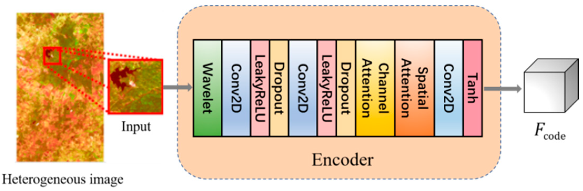
Set up encoders and for the and domains, respectively, to extract the features from the heterogeneous images and . The structure of both encoders is identical, consisting of a wavelet layer, convolutional layers, and attention mechanism layers, but their weights are distinct. The structure diagram of the encoder is shown in Figure 2. The wavelet layer is used to extract image texture information and improve image topology representation. The convolutional layer refines the extracted texture information further. The attention mechanism simulates the correlation between distinct pixels and different bands, balances the influence of various regions, and guides the network’s attention to areas of interest, therefore enhancing effective information and suppressing invalid characteristics. The two encoders can finally obtain an accurate latent space representation of the input images and after iterative training of the network.
For the encoder, the image is first input to the wavelet transform layer. The input image is then subjected to a wavelet transform to decompose the original image into four sub-images. The output of the wavelet transform layer, , is obtained by connecting the sub-images along the channel direction. is input into two consecutive sets of Conv modules to get feature . Among them, each group of Conv modules consists of a layer of 2D convolution operation, a layer of activation operation using a nonlinear activation function LeakyReLU with a parameter of 0.3, and a layer of Dropout operation with a parameter of 0.2. Then, our proposed channel attention module and spatial attention module receive the feature . The attention modules assign larger weights to channels and regions of interest, suppress unnecessary information, and obtain the feature . Finally, feature is subjected to a layer of convolution operation and a layer of activation operation with a nonlinear activation function tanh to yield a latent space representation . The input image block can get the feature through the encoder , and the input image block can get the feature through the encoder .
- (2)
- Decoder
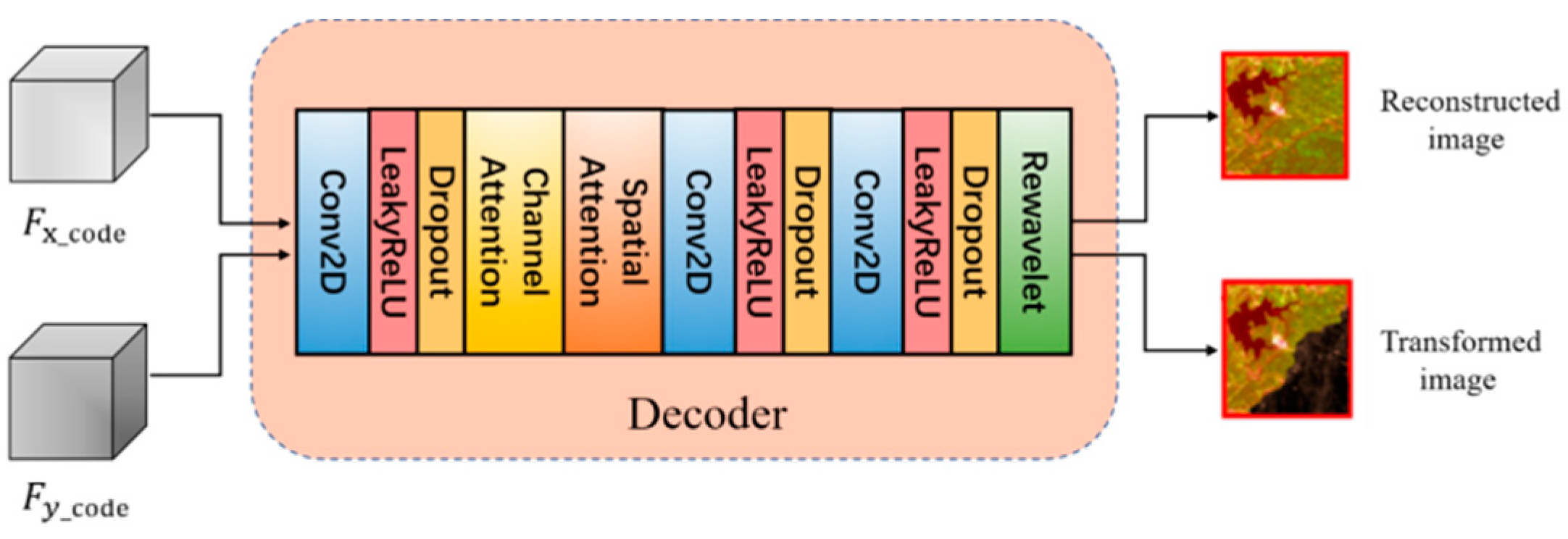
Set the and decoders for the and domains, respectively. The latent space representation is reconstructed into the original image, and the source domain image is transformed into the target domain image. The two decoders have the same structure but do not share weights and consist of convolutional layers, attention mechanism layers, and inverse wavelet transform layers. A schematic diagram of the structure of the decoder is shown in Figure 3. Convolutional layers and attention mechanisms are used to aggregate local information and restore detailed features and spatial dimensions of images. For the final reconstruction of the image, the inverse wavelet transform layer is used to recover as much of the original image’s style and texture structure information as possible, so that the result closely resembles the original. Under the constraint of reconstruction loss, the decoder can get an output that is closer and closer to the original image.
For the decoder, the latent space representation is first input into a set of convolution modules to initially restore the details of the target image. The obtained features are then fed into the attention module for further screening of important features such as image edge information. Two sets of convolution modules are then applied to the output of the attention module to aggregate the local image information and yield high-level features . Among them, each group of Conv modules includes a layer of 2D convolution operation, a layer of activation operation using a nonlinear activation function LeakyReLU with a parameter of 0.3, and a layer of Dropout operation with a parameter of 0.2. Finally, the feature is input into the inverse wavelet transform layer, which performs the operation of reconstructing the sub-image into the original image and obtains the decoder’s output image . The latent space feature can obtain the reconstructed image of the original domain through the decoder , or input the decoder to convert the image domain to obtain the converted image . Similarly, the latent space feature can obtain the reconstructed image of the original domain through the decoder , or input the decoder to convert the image domain to obtain the converted image .
We only set three convolution layers in both the encoder and decoder since the training samples are insufficient and a network that is too deep will result in overfitting and a reduction in accuracy. Therefore, we employ a shallower network to obtain a higher performance. In the experiment, we also show the effect of different convolution layers on the detection results. A well-trained network can transform the image domain, allowing it to use a homogeneous method for change detection in the same domain. The final change map is generated by combining the results from both domains. According to Formula (3), use , , , and to calculate the change detection result map :
where denotes the number of channels in the image , denotes the number of channels in the image , and represents the Otsu method. The Otsu method divides the image into two parts using the concept of clustering so that the gray value difference between the two parts is the greatest and the gray value difference between each part is the smallest. The variance is calculated to find an appropriate gray level to divide. It is easy to calculate, unaffected by image brightness and contrast, and has a high level of robustness.
3.3. Wavelet Transform Module
Wavelet transform can decompose image information using low-pass and high-pass filters, and it is capable of powerful multi-resolution decomposition. By filtering in the horizontal and vertical directions, 2D wavelet multi-resolution decomposition can be accomplished for 2D images. A single wavelet decomposition can produce four sub-bands: LL, HL, LH, and HH. Among them, the LL sub-band is an approximate representation of the image, the HL sub-band represents the horizontal singular characteristic of the image, the LH sub-band represents the vertical singular characteristic of the image, and the HH sub-band represents the diagonal edge characteristic of the image. Inspired by this, we apply the 2D Haar wavelet transform to the network’s first layer, which serves as the front end for the two encoders. The input image is then decomposed into four sub-images in order to obtain the original image’s details in all directions. In this way, we can capture the structural features of the image and focus on highlighting the image’s texture information.
Specifically, we perform a Haar wavelet transform on each band of the input image , where is the image size and is the number of channels. In this way, each band of the original image generates four sub-bands respectively, representing the information from different directions of the image. Then the generated sub-images are connected according to the channel direction to generate a new image with size and the number of channels . The image is then sent to the succeeding convolution layer to extract features. Because the bi-temporal heterogeneous images usually have different channel numbers, the channel numbers of new images generated after wavelet transform are also different. However, the two images can be processed by the convolution layer using the same number of filters, and the output features with the same number of channels can be obtained. As a result, we adjust the number of channels of output features by adjusting the number of filters in the network’s convolutional layer. A schematic diagram of the structure of the wavelet transform module is shown in Figure 4. We utilize all sub-images, which not only provide a clearer description of the image’s details but also prevent the information loss caused by conventional subsampling, which is advantageous for image reconstruction. It is worth mentioning that we add an inverse wavelet transform layer at the end of the network to reconstruct the image and restore the overall image representation. For the 2D Haar wavelet, the four kernels , , , and defined by Equation (4) are used for the wavelet transform [50].
When an image undergoes 2D Haar wavelet transformation, the th value of the transformed image is defined as:
3.4. Attention Module
- (1)
- Channel attention module
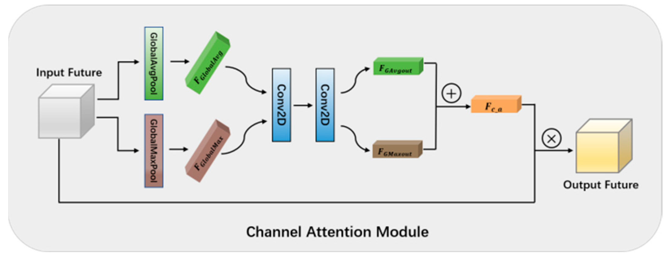
All of the RS images in the three datasets used in this paper have multiple bands. In the study of heterogeneous CD, we discovered that the majority of methods only enhanced the spatial features and usually utilized a simple convolution operation to describe the connection between channels, without effectively defining the channels’ internal dependencies. In addition, we performed wavelet transform on each band and connected the generated sub-bands according to the channel direction. Each channel of features extracted by subsequent convolutional layers represents a distinct meaning. As a result, a channel attention module must be introduced to adaptively adjust the feature response value of each channel, pay attention to which layers at the channel level will have stronger feedback capabilities, and model the internal dependencies between channels.
A schematic diagram of the structure of the channel attention module is shown in Figure 5. Each channel of the feature map responds differently to the image’s features, reflecting different information in the image. We also need to selectively focus on the various channels of the feature map to concentrate on the features of the changing region. We employ global average pooling and global max pooling to compress the spatial dimension of the input feature in order to calculate the channel attention matrix and minimize network parameters. The degree information of the object can be learned using the average pooling method, and its discriminant features can be learned using the max pooling method. The combined use of two pooling methods can improve image information retention. Therefore, we input the feature into the GlobalAveragePooling2D layer and the GlobalMaxPooling2D layer and calculate the mean value and maximum value of each channel of the input features, respectively, to get two feature descriptions and . Among them, and aggregate the average and maximum information of the input feature in spatial dimension, respectively. Then, and are fed into two convolution layers, which are used to further process these two different spatial contexts. The two convolution layers have 4 and 50 filters of size . The first convolutional layer employs 4 filters to reduce the number of parameters and prevent network overfitting. The second convolutional layer employs 50 filters to ensure that the output feature has the same number of channels as the input feature. The two output features are then added element by element and the weight coefficient is obtained by a Sigmoid activation function. Finally, multiply the weight coefficient with the input feature to get the scaled new feature. The information we care about is enhanced in this new feature, while the less important information is suppressed.
- (2)
- Spatial attention module
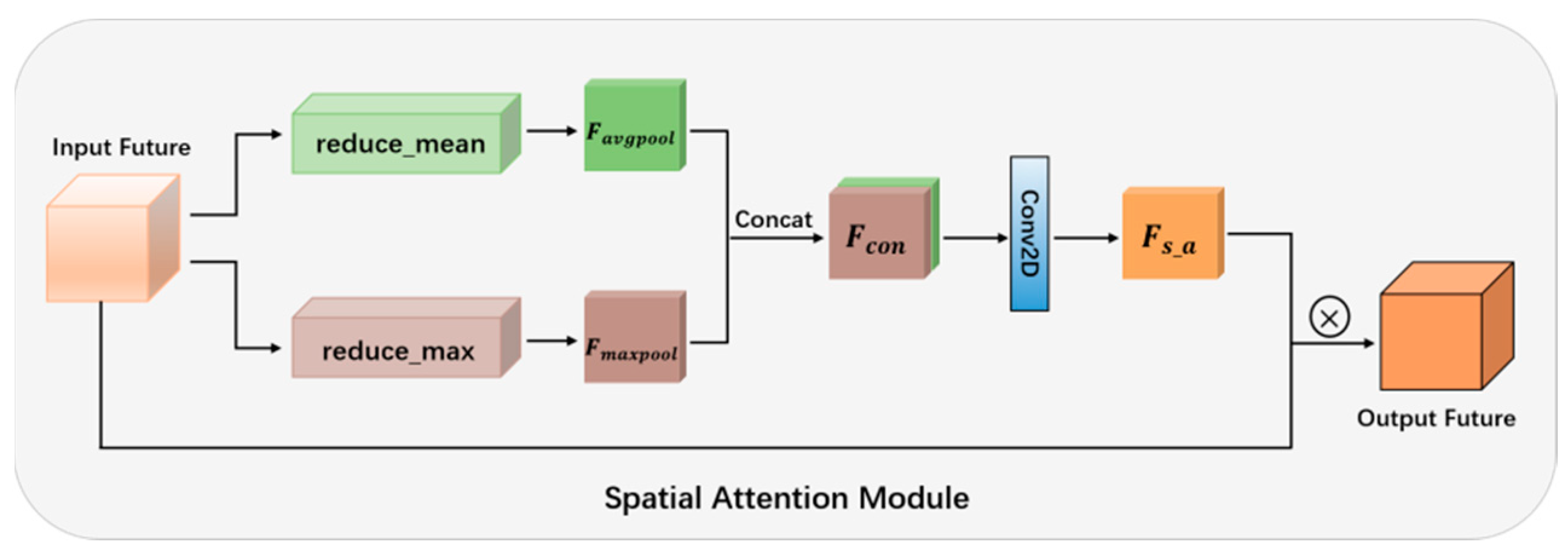
When we perceive an image, the first thing we notice is not the entire image, but a portion of it; this portion is the image’s focal point. The spatial features of images contain rich location information, and the importance of spatial location information varies depending on the task, with the area related to the task receiving more attention. Therefore, the spatial attention module is introduced to process the most important parts of the network while suppressing uninteresting regional features.
A schematic diagram of the structure of the spatial attention module is shown in Figure 6. The spatial attention module, unlike the channel attention module, focuses on where the information of interest is located and can effectively model the spatial relationships within the feature. The spatial attention module is complementary to the channel attention module. After the input features are processed by the channel attention module and the spatial attention module, they can not only enhance the features we are interested in, but also highlight the areas related to the task. In order to compute the spatial attention matrix, the channel dimensions of the input features need to be compressed first. For channel compression, we employ both average and max pooling, as with the channel attention mechanism. The two methods of pooling can achieve information complementation while retaining image features. Specifically, the input feature is first pooled using reduce_mean and reduce_max along the channel direction to produce two spatial features. The feature is then obtained by connecting these two spatial features according to the channel direction. can highlight the information area. Then, is input into the convolution layer for the calculation to obtain the spatial attention matrix . The convolutional layer has a filter of size and is activated by the sigmoid function. The spatial attention matrix can then be multiplied with the input feature to yield the output feature of the spatial attention module. This enables us to concentrate on regions of greater interest and improve the performance of change detection.
We apply the attention module to the encoder and decoder to better encode and restore the image’s critical parts, therefore significantly enhancing the performance of the network.
3.5. Network Training Strategy
The network proposed in this paper takes the form of two inputs. The two-phase heterogeneous RS image training sample blocks and are input into the proposed network framework in the form of patches for unsupervised training. Inspired by [32], this paper comprehensively uses four loss functions , , , and to train the network. To achieve accurate image domain conversion, the loss function is used to constrain the commonality of the encoder’s latent space, ensuring that the statistical distribution of the two encoders’ output features is more consistent. Because is calculated based on the input images and latent features, it is only used to train two encoders. , , and loss functions constrain image source domain reconstruction, image cycle reconstruction, and image cross-domain conversion, respectively. The weighted sum of these three loss functions is used to obtain , which is then used to update the parameters of the entire network. In each epoch of training, is used to update the encoder parameters first, and then is used to update the parameters of the entire network.
According to Equation (6), the parameters of encoders and are updated using the loss function . This loss function restricts the commonality of encoder-generated features, enabling image domain transformation.
where represents the image’s affinity matrix, which is used to represent the probability of similarity between two points, and the pixel similarity relationship obtained from the affinity matrix is used to reduce the influence of changing pixels [51]. represents the number of channels of , and represents the number of pixel points of .
According to Formula (7), the parameters of the entire change detection network are updated using the loss function .
where represents the number of pixel points of , represents the change prior, and , , and represent the preset weight coefficients. In the experimental section, we discuss the effect of various weight coefficients on the network’s accuracy.
Based on the above research, Algorithm 1 summarizes the proposed bitemporal heterogeneous RS image change detection process.
| Algorithm 1 Change detection in bi-temporal heterogeneous RS image |
| Input: Bi-temporal heterogeneous RS images and , training epoch, learning rate and patch size. |
| Output: Change map; |
| Initialization: Initialize all network parameters; |
| While, do: |
| 1: Input the bi-temporal heterogeneous RS images into the change detection network; |
| 2: Encode heterogeneous images and with encoders and to obtain latent space features and ; |
| 3: Use the decoder to reconstruct the image of the latent space feature , and perform image transformation of the latent space feature ; use the decoder to perform image transformation on the latent space feature , and perform image reconstruction on the latent space feature ; |
| 4: Calculate the loss function according to Formulas (6) and (7), and perform the Backward process; |
| End While |
| According to Formula (3), obtain the final change detection result map . |
4. Experiment and Analysis
All programs in this article were written in Python 3.6. The neural network was built with TensorFlow. All experiments were done on a computer configured with Intel Core i7, GeForce RTX 3070 Laptop, and Windows 10.
4.1. Datasets
- (1)
- Forest fire in Texas
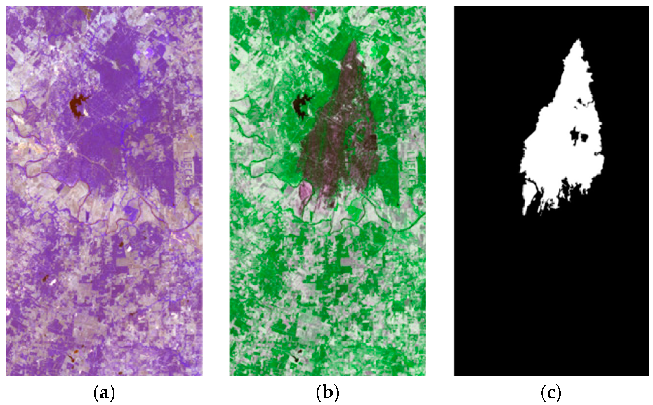
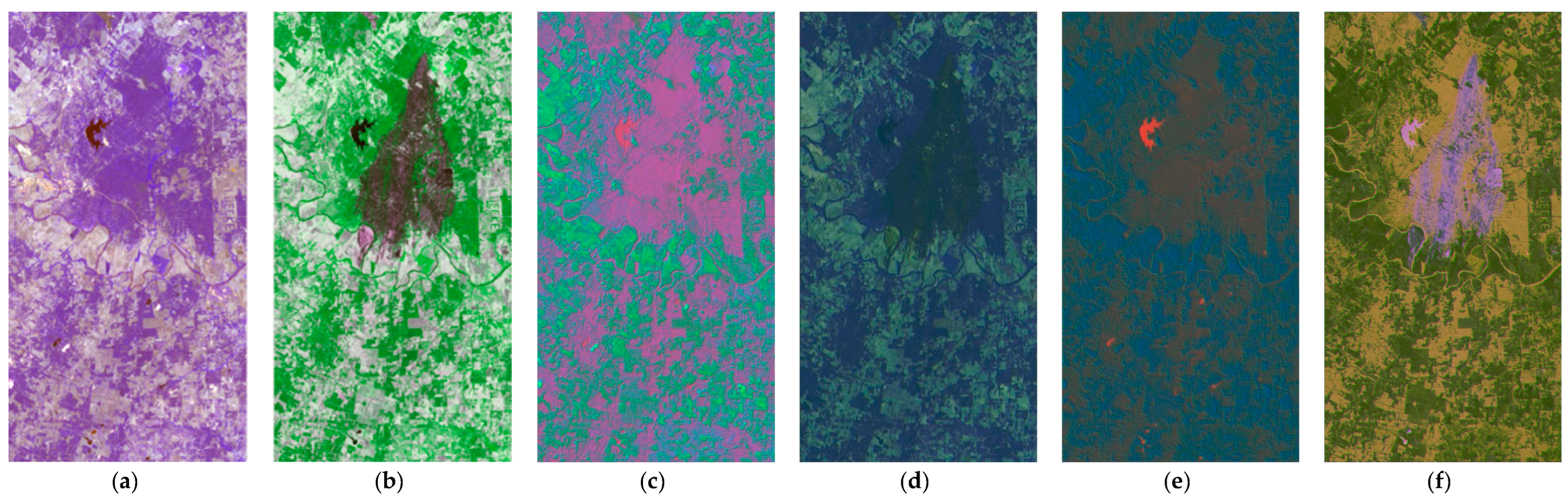
The “Forest fire in Texas” dataset [52] focuses on forest fires in Bastrop County, Texas, USA. It is comprised of two bi-temporal multispectral optical images captured at different times. The pre-fire image was taken by Landsat 5 TM in September 2011, and the post-fire image was taken by Earth Observing-1 Advanced Land Imager (EO-1 ALI) in October 2011. The two registered images have a resolution of , with 7 and 10 bands, respectively. Figure 7 shows pseudo-color images of the dataset and their corresponding ground truth images.
- (2)
- Flood in California
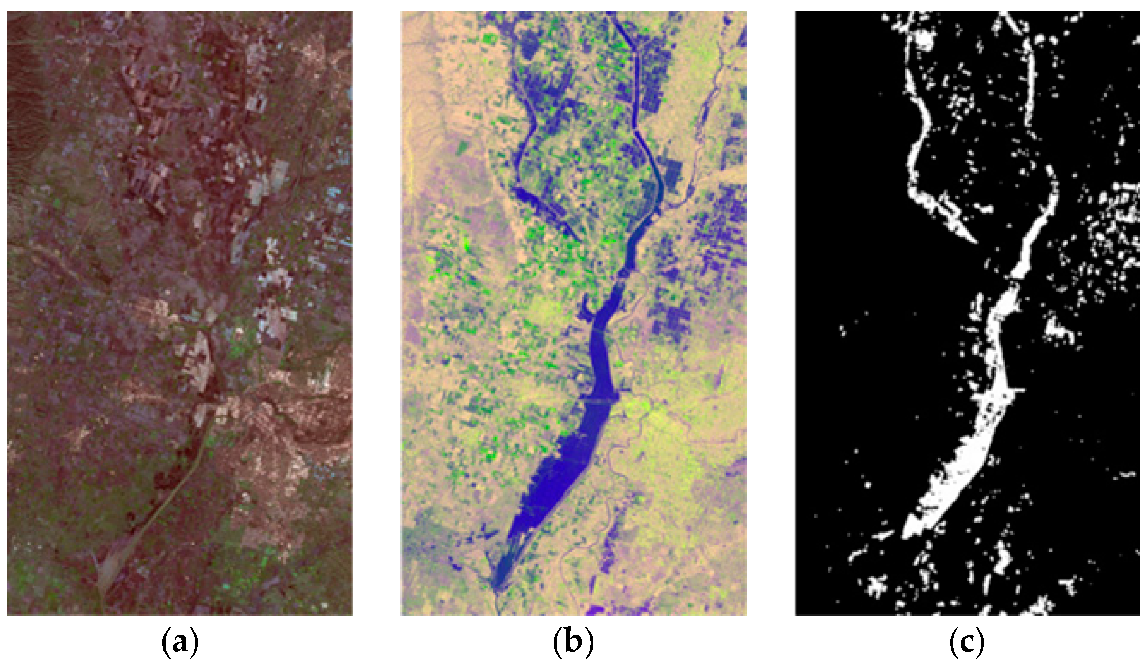
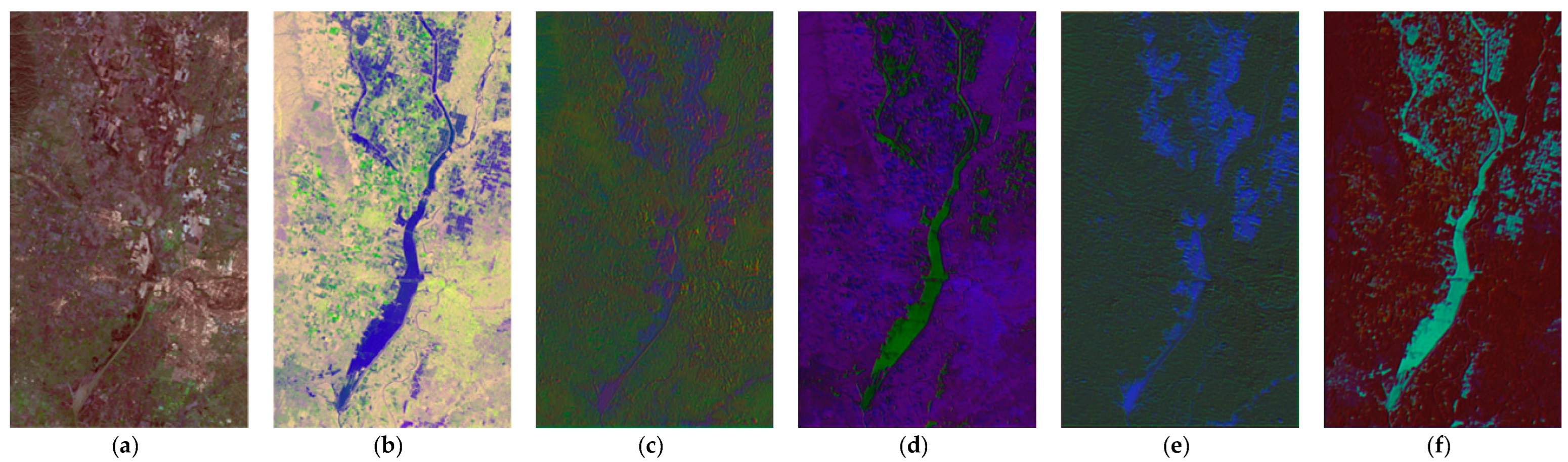
The “Flood in California” dataset [53] focuses on flooding in Sacramento, Yuba, and Sutter counties in California, USA. It is comprised of two multispectral and synthetic aperture radar images captured at different times. The multispectral image has a size of 875 × 500 × 11 and was taken by Landsat 8 on 5 January 2017. The SAR image size is 875 × 500 × 3, acquired by Sentinel-1A on 18 February 2017, recorded in polarized VV and VH, and enhanced with the ratio between the two intensities as the third channel. The original size of these images is 3500 × 2000. The images were resampled to 875 × 500 using the bilinear interpolation method to reduce the computational complexity. Figure 8 shows pseudo-color images of the dataset and their corresponding ground truth images.
- (3)
- Lake overflow in Italy
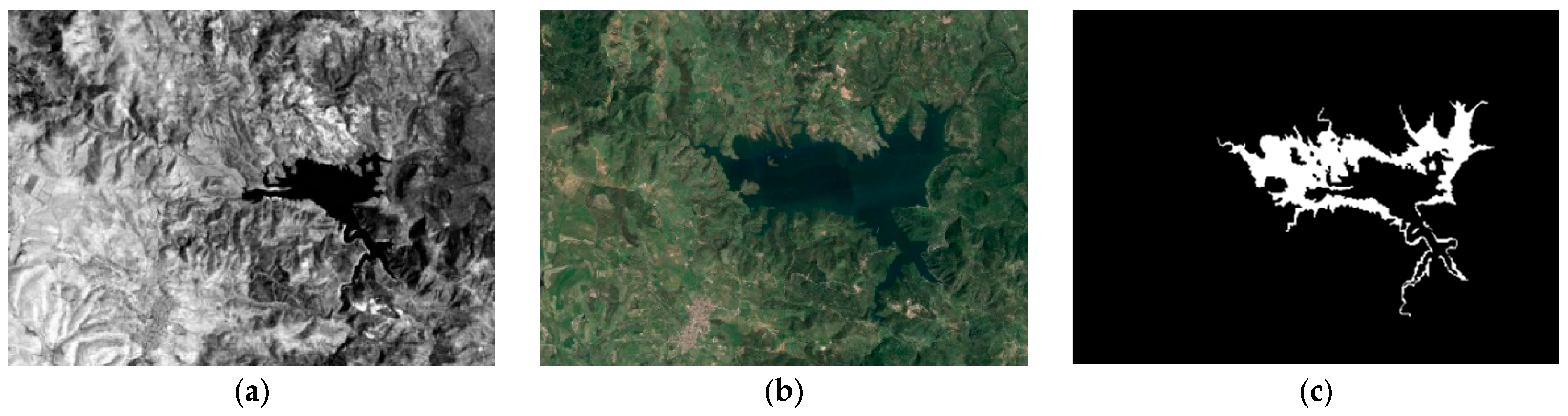
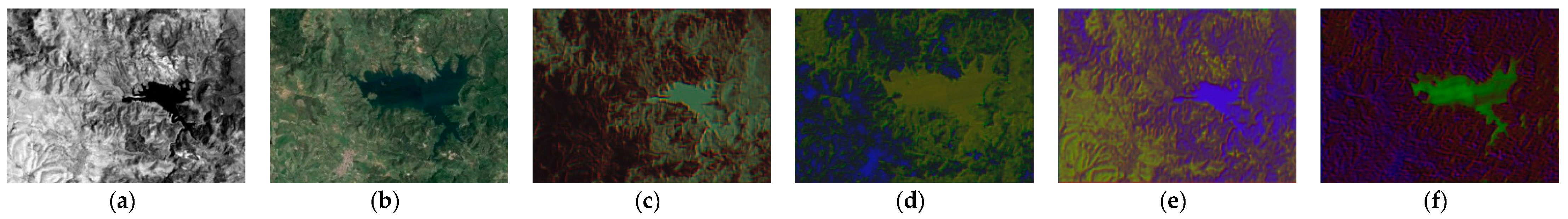
The “Lake overflow in Italy” dataset [20] focuses on the lake overflow in Sardinia, Italy. It consists of a pair of near-infrared images and optical images taken at different times. The pre-overflow image was taken by Landsat 5 in September 1995, and the post-overflow image was taken by Google Earth (GEt2) in July 1996. The size of the two registered images is with one and three bands, respectively. Figure 9 shows the two images of the dataset and their corresponding ground truth images.
4.2. Parameter Settings
- (1)
- Patch size
The amount of information contained is determined by the difference in the size of the input block, and the amount of information determines the number of features to be extracted and the correlation between the features. This paper conducted experimental comparisons on the three sets of test datasets using input data blocks of various sizes to compare the influence of neighborhood blocks of different scales on the algorithm model. Figure 10 shows the performance of our CD algorithm on the three datasets ranging from to . The statistical graph shows that the optimal block size for the three datasets was .
- (2)
- The learning rate
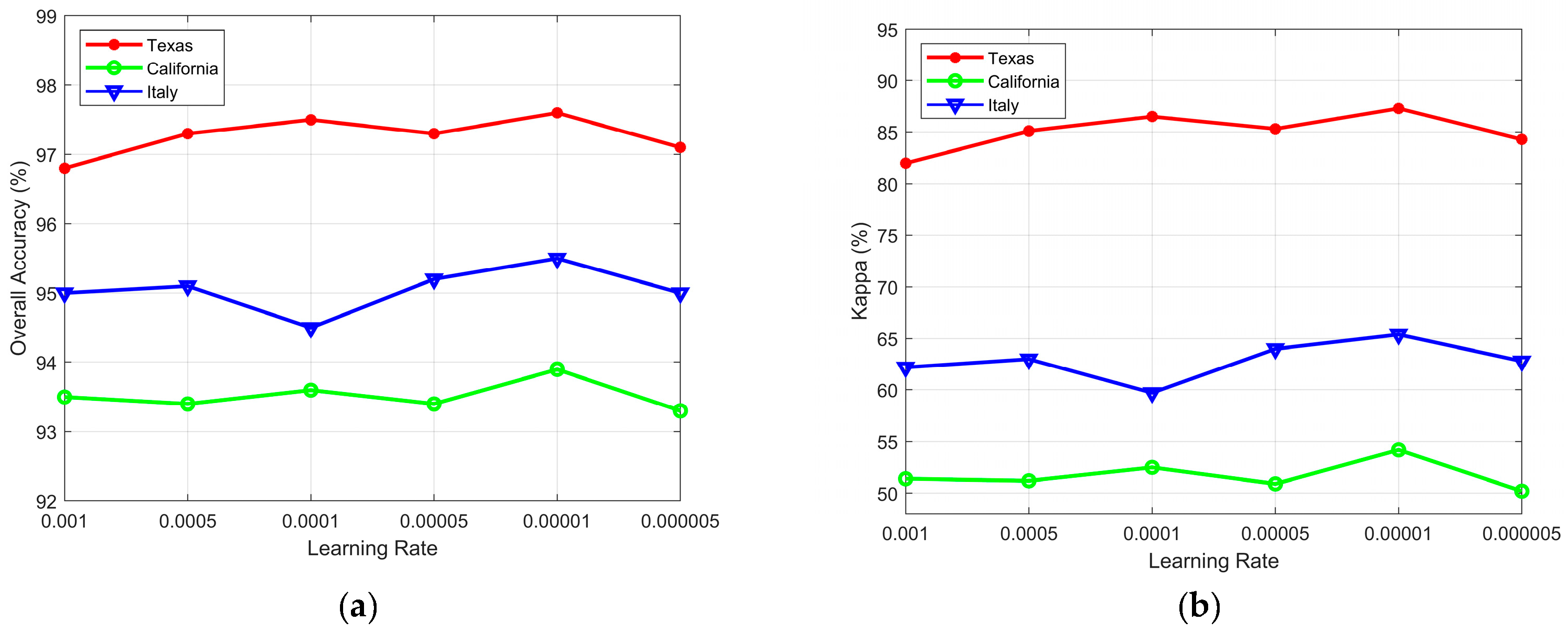
Learning rate is an important hyperparameter in deep learning since it determines whether and when the objective function can converge to the local minimum. It explains how to use the gradient of the loss function to tune the network weight hyperparameters in gradient descent. Figure 11 shows the performance of the CD algorithm on the three datasets under different learning rates. The statistical graph shows that the optimal learning rate for the three datasets was 0.00001.
- (3)
- The Loss function parameter
In Formula (7) of Section 3, we utilize the weighted sum of the loss functions , , and to calculate the overall loss function . To balance the influence of different loss functions on network training, hyperparameters , , and determine the contribution of , , and to the total loss function, respectively. We set the following values for , , and : (0.1, 0.1, 0.1), (0.2, 0.1, 0.1), (0.1, 0.2, 0.1), (0.1, 0.1, 0.2) and (0.2, 0.2, 0.2). Figure 12 shows the performance of the proposed algorithm for CD of the three datasets under various hyperparameter combinations. The statistical graph shows that the optimal hyperparameter combination of the three datasets was , , and : (0.1, 0.2, 0.1).
- (4)
- The number of convolution layers
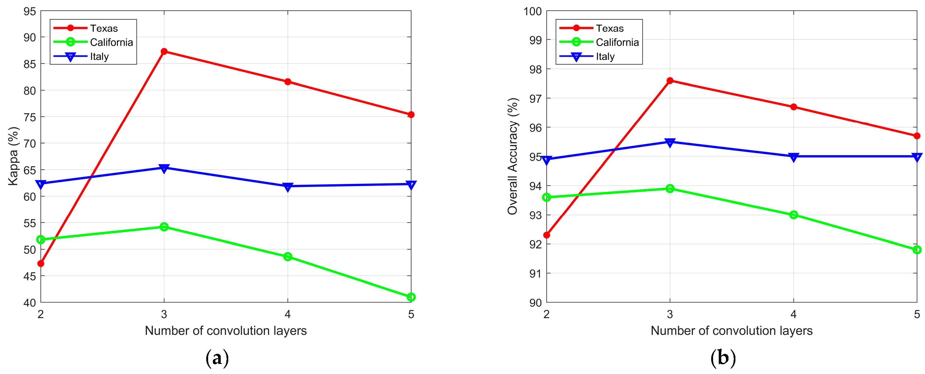
The setting of the number of convolution layers affects the performance of the network. Because our training samples are insufficient, a network that is too deep will result in overfitting, which will degrade the model’s performance. The shallow network cannot extract the deep semantic features, which limits the network’s ability to learn the meaningful feature representation and impacts the accuracy of detection. Figure 13 shows the performance of the proposed algorithm for CD of the three datasets under different numbers of convolution layers. The statistical graph shows that the optimal number of convolution layers for the three datasets was three. Moreover, when the number of convolution layers is set to two, the performance of the algorithm on the Texas dataset decreased significantly. Because the dataset has a high resolution, a network that is too shallow cannot learn the precise feature representation.
4.3. Analysis of Results
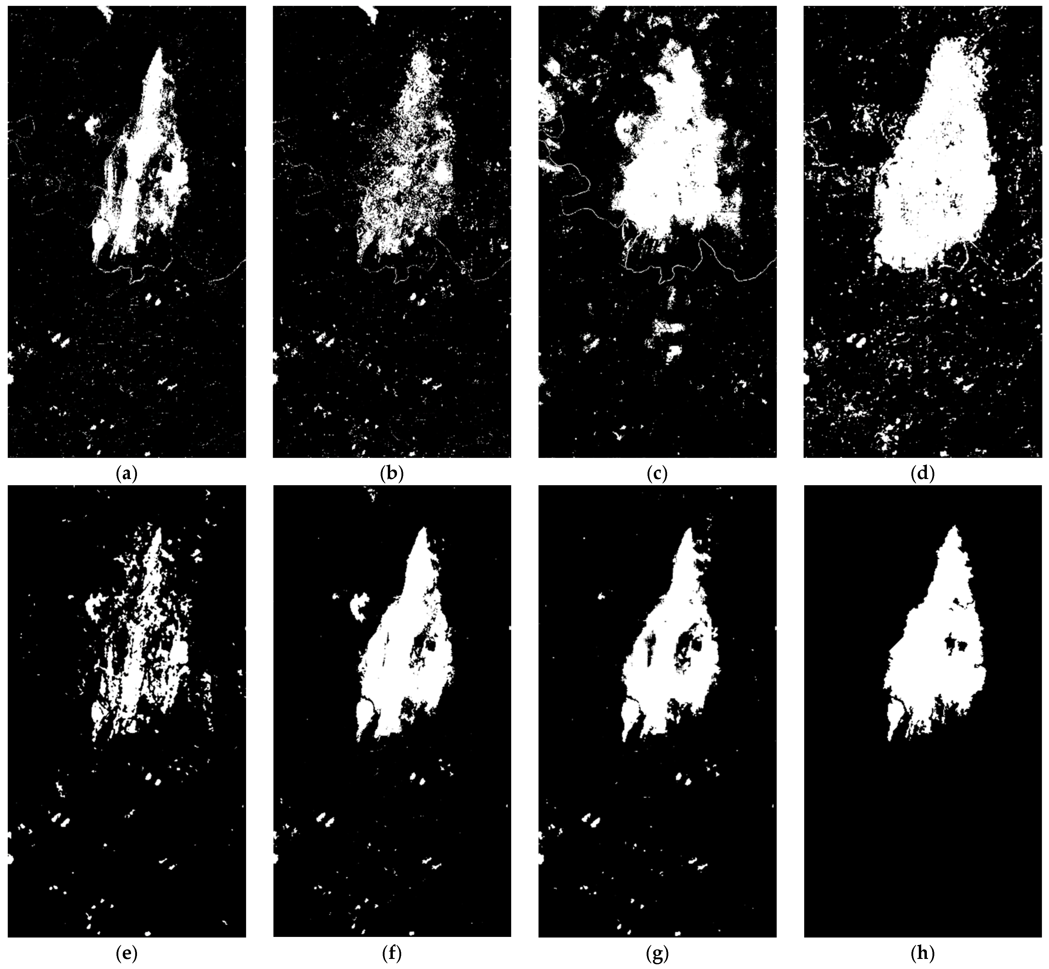
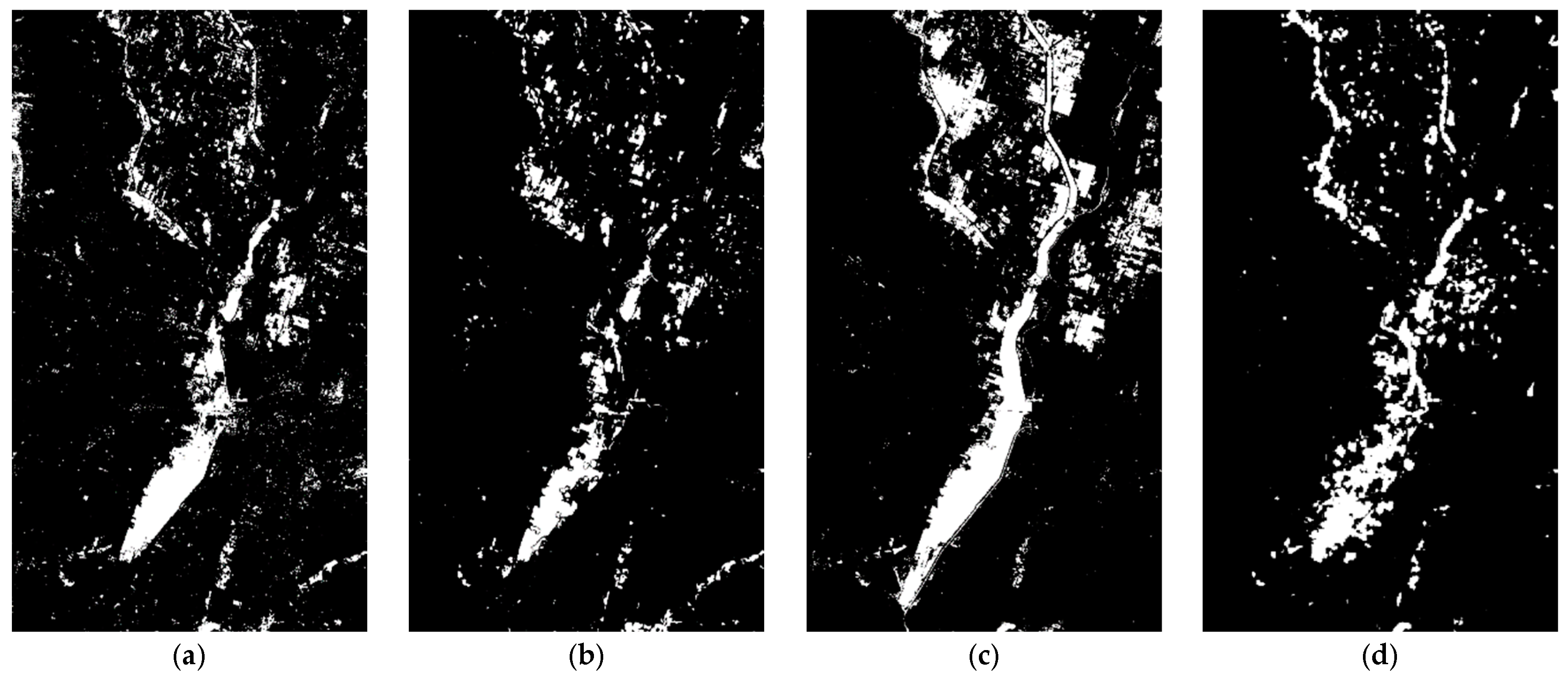
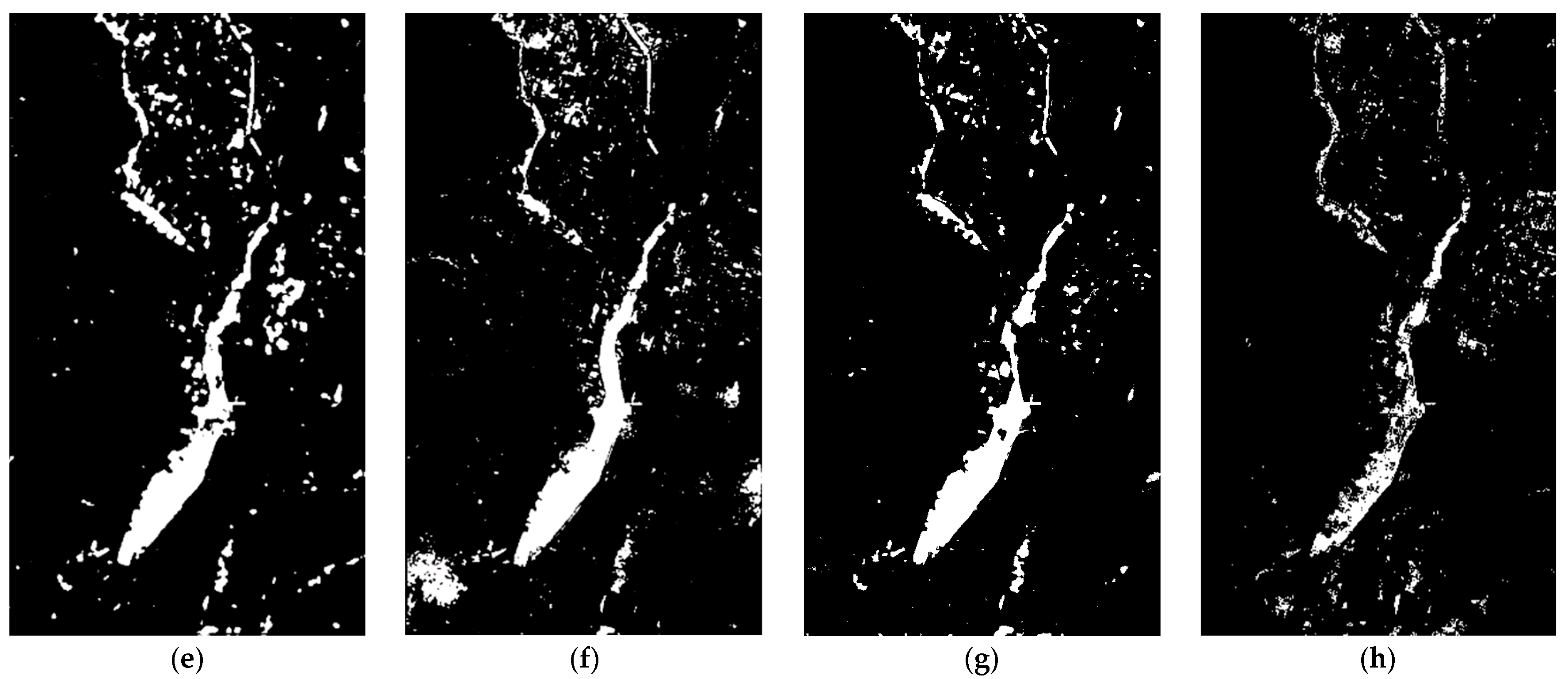
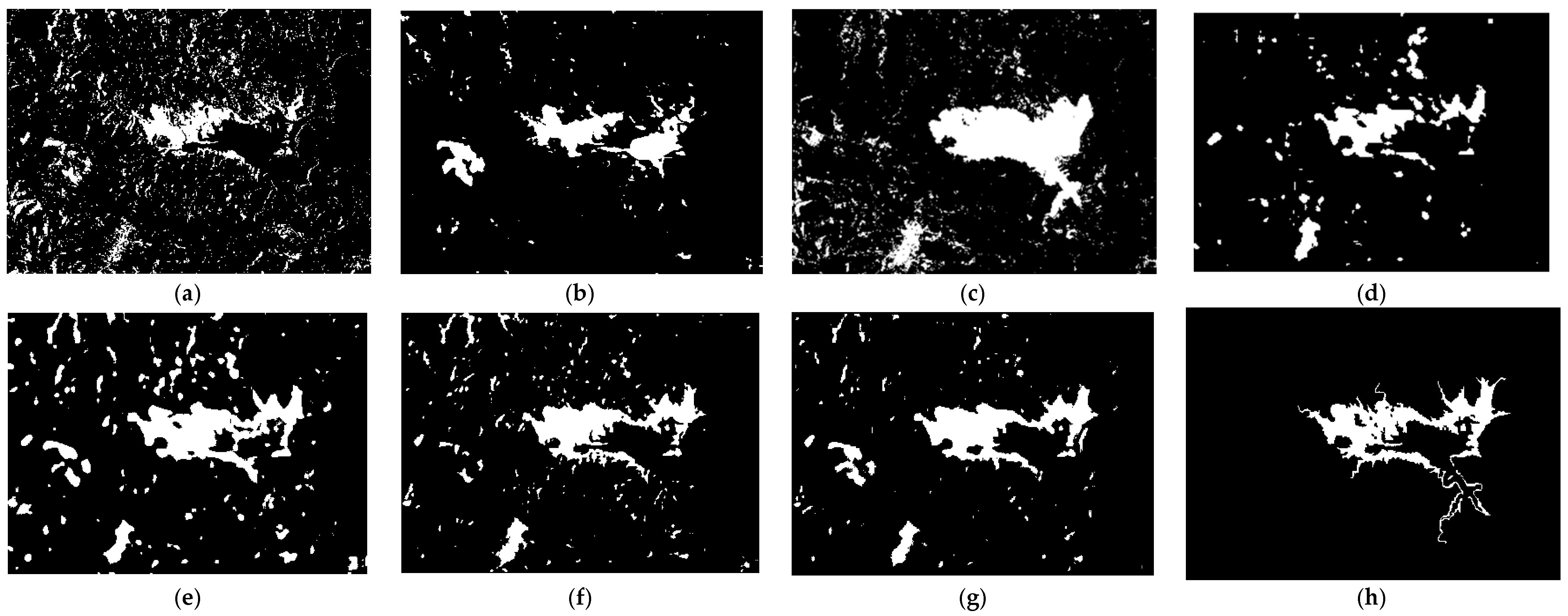
In order to verify the effectiveness of the algorithm, we conducted experiments using three sets of bitemporal heterogeneous RS datasets and compared the results of the algorithm with the other five algorithms. These six algorithms include the Deep Image Translation with an Affinity-Based Change Prior (ACE-Net) [51], Conditional Adversarial Network (CAN) [25], Deep Convolutional Coupling Network (SCCN) [24], Non-local Patch Similarity-based Graph (NPSG) [20], Improved Non-local Patch-based Graph (INLPG) [54], and Code-aligned autoencoders (CAA) [32]. Among them, ACE-Net, CAN, SCCN, and CAA are all unsupervised deep neural network methods. The results of the experiments were compared to the optimal parameters presented in the literature. Both NPSG and INLPG performed heterogeneous RS image change detection based on non-local patch similarity. To ensure the fairness of the comparative experiments, the experiments were conducted using parameter values that corresponded to the best experimental results presented in the references. Figure 14, Figure 15 and Figure 16 show the results of change detection for the three datasets: Forest fire in Texas, Flood in California, and Lake overflow in Italy using different algorithms. Figure 14h, Figure 15h and Figure 16h show the ground truth of the three datasets.
For the Forest fire in Texas dataset, Figure 14 shows that, when compared to ground truth, the ACE-Net, CAN, and INLPG algorithms were insufficient in detecting the changed areas. Their result maps contained more false negative pixels, and the CAN algorithm’s result map had more noise points. In the conversion of the image feature space, the ACE-Net and CAN algorithms lost some features, resulting in the omission of some changes. Although the CAA algorithm produced good results, the method proposed in this paper had fewer error points in the unchanged region. There were too many false positive pixels in the results of the SCCN and NPSG algorithms. In contrast, the method proposed in this paper yielded a result map with fewer misclassified points that is closer to the ground truth.
For the Flood in California dataset, Figure 15 demonstrates that the ACE-Net result map contained more noise points, whereas the CAN, SCCN, NPSG, and CAA result maps contained more false positive pixels. The CAA algorithm did not fully consider the texture structure of the image, resulting in some conversion errors. The influence of changed regions was not fully considered by the CAN and SCCN algorithms, resulting in the inaccurate conversion of unchanged pixels. The NPSG algorithm had inadequate capacity to model complicated regions. The INLPG algorithm produced satisfactory results. However, the method proposed in this paper had fewer misclassification points.
For the Lake overflow in Italy dataset, Figure 16 demonstrates that the result map of the ACE-Net algorithm had more noise. The result maps produced by the CAN, SCCN, and INLPG algorithms contained more false positives. The NPSG algorithm was insufficient to detect the changing region. Although the CAA algorithm produced good results, the method proposed in this paper had some advantages, including fewer errors and clearer boundaries.
We conducted feature visualization of the attention module to test the effectiveness of the attention mechanism. Figure 17, Figure 18 and Figure 19 demonstrates the output features of the attention module in the encoder and decoder for the three datasets. As shown in the figure, the attention mechanism can highlight the changing region and improve the feature representation of the region of interest, thereby enhancing the ability of the network to capture fine changes and effectively improving the accuracy of CD.
4.4. Ablation Experiment
The method proposed in this paper focuses on adding wavelet transform and attention modules to the network to extract topological structure information from heterogeneous RS images. The ablation analysis was performed on three datasets to validate the rationality and effectiveness of the wavelet transform and attention mechanism proposed by the algorithm in this paper. Table 4 shows the objective evaluation metrics for the three datasets. The evaluation indicators in the table demonstrate that the wavelet transform and attention mechanism proposed by us can improve the accuracy of the heterogeneous RS image CD algorithm and significantly improve network performance.
In addition, we also performed an ablation experiment using only one attention module in order to confirm the efficacy of using both channel and spatial attention mechanisms. Table 5 shows the objective evaluation metrics for the three datasets. The evaluation indicators in the table demonstrate that utilizing two attention modules concurrently can effectively improve the accuracy of change detection.
We performed a feature visualization comparison between the proposed method and the original neural network to demonstrate that the proposed method can highlight the topological structure information of the images. Figure 20, Figure 21 and Figure 22 show the output features of the proposed method and the original neural network in the three datasets. As shown in the figure, the method proposed in this paper can highlight the changing region while also effectively capturing the image’s topological structure features. As a result, the error of image conversion can be reduced and the performance of change detection can be effectively improved.
5. Conclusions
This paper proposes a topological structure coupling-based method for detecting changes in heterogeneous RS images. First, a neural network framework for CD in heterogeneous RS images was introduced, which realizes the mutual conversion of heterogeneous image domains through the network, thereby calculating the difference map in the same domain. The final change result map is generated by combining the difference maps calculated in two different image domains, which greatly improves change detection accuracy. Second, we employ the wavelet transform to extract image texture structure features, which are primarily represented by the spatial distribution of high-frequency information on the image. The combination of high-frequency and low-frequency information improves the topological features of the image, reduces interference caused by different feature spaces, and improves the network’s ability to capture fine changes. The channel attention mechanism and the spatial attention mechanism are then used to assign more weights to the region of interest while suppressing unnecessary features. The network can focus on the texture information of interest and suppress the difference between images from different domains by using an organic combination of wavelet, channel attention module, and spatial attention module. Then, the algorithm proposed in this paper was tested on three datasets. The experimental results demonstrated that the proposed algorithm for heterogeneous RS image change detection takes into account the relationship between image topological structures and improved network performance.
The proposed method also has some limitations. For example, the advanced semantic features of the images are not fully utilized during the image domain conversion process. Especially for changing regions, the completeness of semantic content ensures that the changes are accurately identified. The consistency of semantic content can also reduce change false detection in unchanged regions. Furthermore, a more robust supervised homogeneous CD network was not used to generate the final change map after the realization of image feature space conversion, which limits the performance of change detection to a certain extent. More focus will be placed in future work on the use of advanced semantic features of images to reduce errors in image conversion, as well as the use of a deep neural network to generate the final change map to improve the accuracy of change detection. The source code of the proposed method can be downloaded from https://github.com/xiazhi-1090/TSCNet.
Author Contributions
Conceptualization and methodology, X.W.; Formal analysis and writing—original draft preparation, W.C.; Investigation, validation, and data curation, Y.F.; Supervision and writing—review and editing, R.S. All authors have read and agreed to the published version of the manuscript.
Funding
This research was funded by the National Natural Science Foundation of China (Grant No. 41971388), the China Postdoctoral Science Foundation (Grant No. 2022M723222), and the Innovation Team Support Program of Liaoning Higher Education Department (Grant No. LT2017013).
Data Availability Statement
Not applicable.
Acknowledgments
The authors would like to thank the editors and the reviewers for their valuable suggestions.
Conflicts of Interest
The authors declare no conflict of interest.
References
- Gong, J.; Haigang, S.; Guorui, M.; Qiming, Z. A review of multi-temporal remote sensing data change detection algorithms. Int. Arch. Photogramm. Remote Sens. Spat. Inf. Sci. 2008, 37, 757–762. [Google Scholar]
- Luppino, L.T.; Anfinsen, S.N.; Moser, G.; Jenssen, R.; Bianchi, F.M.; Serpico, S.; Mercier, G. A clustering approach to heterogeneous change detection. In Scandinavian Conference on Image Analysis; Springer: Cham, Switzerland, 2017; pp. 181–192. [Google Scholar]
- Liu, Z.; Li, G.; Mercier, G.; He, Y.; Pan, Q. Change detection in heterogenous remote sensing images via homogeneous pixel transformation. IEEE Trans. Image Process. 2017, 27, 1822–1834. [Google Scholar] [CrossRef] [PubMed]
- Lambin, E.F.; Strahlers, A.H. Change-vector analysis in multitemporal space: A tool to detect and categorize land-cover change processes using high temporal-resolution satellite data. Remote Sens. Environ. 1994, 48, 231–244. [Google Scholar] [CrossRef]
- Nielsen, A.A.; Conradsen, K.; Simpson, J.J. Multivariate alteration detection (MAD) and MAF postprocessing in multispectral, bitemporal image data: New approaches to change detection studies. Remote Sens. Environ. 1998, 64, 1–19. [Google Scholar] [CrossRef] [Green Version]
- Celik, T. Unsupervised change detection in satellite images using principal component analysis and k-means clustering. IEEE Geosci. Remote Sens. Lett. 2009, 6, 772–776. [Google Scholar] [CrossRef]
- Dalla Mura, M.; Prasad, S.; Pacifici, F.; Gamba, P.; Chanussot, J.; Benediktsson, J.A. Challenges and opportunities of multimodality and data fusion in remote sensing. Proc. IEEE 2015, 103, 1585–1601. [Google Scholar] [CrossRef] [Green Version]
- Ghamisi, P.; Rasti, B.; Yokoya, N.; Wang, Q.M.; Hofle, B.; Bruzzone, L.; Bovolo, F.; Chi, M.M.; Anders, K.; Gloaguen, R.; et al. Multisource and multitemporal data fusion in remote sensing: A comprehensive review of the state of the art. IEEE Geosci. Remote Sens. Mag. 2019, 7, 6–39. [Google Scholar] [CrossRef] [Green Version]
- Su, L.; Gong, M.; Zhang, P.; Zhang, M.; Liu, J.; Yang, H. Deep learning and mapping based ternary change detection for information unbalanced images. Pattern Recognit. 2017, 66, 213–228. [Google Scholar] [CrossRef]
- Gong, M.; Niu, X.; Zhan, T.; Zhang, M. A coupling translation network for change detection in heterogeneous images. Int. J. Remote Sens. 2018, 40, 3647–3672. [Google Scholar] [CrossRef]
- Storvik, B.; Storvik, G.; Fjrtoft, R. On the combination of multi-sensor data using meta-gaussian distributions. IEEE Trans. Geosci. Remote Sens. 2009, 47, 2372–2379. [Google Scholar] [CrossRef]
- Gong, Z.; Maoguo, G.; Jia, L.; Puzhao, Z. Iterative feature mapping network for detecting multiple changes in multi-source remote sensing images. ISPRS J. Photogramm. Remote Sens. 2018, 146, 38–51. [Google Scholar]
- Jensen, J.R.; Ramsey, E.W.; Mackey, H.E.; Christensen, E.J.; Sharitz, R.R. Inland wet land change detection using aircraft MSS data. Photogram. Eng. Remote Sens. 1987, 53, 521–529. [Google Scholar]
- Mubea, K.; Menz, G. Monitoring land-use change in Nakuru (Kenya) using multi-sensor satellite data. Adv. Remote Sens. 2012, 1, 74–84. [Google Scholar] [CrossRef]
- Wan, L.; Xiang, Y.; You, H. A post-classification comparison method for SAR and optical images change detection. IEEE Geosci. Remote Sens. Lett. 2019, 16, 1026–1030. [Google Scholar] [CrossRef]
- Wan, L.; Xiang, Y.; You, H. An object-based hierarchical compound classification method for change detection in heterogeneous optical an d SAR images. IEEE Trans. Geosci. Remote Sens. 2019, 57, 9941–9959. [Google Scholar] [CrossRef]
- Mercier, G.; Moser, G.; Serpico, S.B. Conditional copulas for change detection in heterogeneous remote sensing images. IEEE Trans. Geosci. Remote Sens. 2008, 46, 1428–1441. [Google Scholar] [CrossRef]
- Prendes, J.; Chabert, M.; Pascal, F.; Giros, A.; Tourneret, J.-Y. A new multivariate statistical model for change detection in images acquired by homogeneous and heterogeneous sensors. IEEE Trans. Image Process. 2014, 24, 799–812. [Google Scholar] [CrossRef] [Green Version]
- Ayhan, B.; Kwan, C. A new approach to change detection using heterogeneous images. In Proceedings of the 2019 IEEE 10th Annual Ubiquitous Computing, Electronics & Mobile Communication Conference (UEMCON), New York, NY, USA, 10–11 October 2019; pp. 0192–0197. [Google Scholar]
- Sun, Y.; Lei, L.; Li, X.; Sun, H.; Kuang, G. Nonlocal patch similarity based heterogeneous remote sensing change detection. Pattern Recognit. 2021, 109, 107598–107616. [Google Scholar] [CrossRef]
- Lei, L.; Sun, Y.; Kuang, G. Adaptive local structure consistency-based heterogeneous remote sensing change detection. IEEE Geosci. Remote Sens. Lett. 2020, 2020, 8003905. [Google Scholar] [CrossRef]
- Sun, Y.; Lei, L.; Guan, D.; Kuang, G. Iterative robust graph for unsupervised change detection of heterogeneous remote sensing images. IEEE Trans. Image Process. 2021, 30, 6277–6291. [Google Scholar] [CrossRef]
- Zhang, P.; Gong, M.; Su, L.; Liu, J.; Li, Z. Change detection based on deep feature representation and mapping transformation for multi-spatial -resolution remote sensing images. ISPRS J. Photogram. Remote Sens. 2016, 116, 24–41. [Google Scholar] [CrossRef]
- Liu, J.; Gong, M.; Qin, K.; Zhang, P. A deep convolutional coupling network for change detection based on heterogeneous optical and radar images. IEEE Trans. Neural Netw. Learn. Syst. 2018, 29, 545–559. [Google Scholar] [CrossRef] [PubMed]
- Niu, X.; Gong, M.; Zhan, T.; Yang, Y. A conditional adversarial network for change detection in heterogeneous images. IEEE Geosci. Remote Sens. Lett. 2019, 16, 45–49. [Google Scholar] [CrossRef]
- Wu, Y.; Bai, Z.; Miao, Q.; Ma, W.; Yang, Y.; Gong, M. A classified adversarial network for multi-spectral remote sensing image change detection. Remote Sens. 2020, 12, 2098–2116. [Google Scholar] [CrossRef]
- Jiang, X.; Li, G.; Liu, Y.; Zhang, X.-P.; He, Y. Change detection in heterogeneous optical and SAR remote sensing images via deep homogeneous feature fusion. IEEE J. Sel. Top. Appl. Earth Obs. Remote Sens. 2020, 13, 1551–1566. [Google Scholar] [CrossRef] [Green Version]
- Li, X.; Du, Z.; Huang, Y.; Tan, Z. A deep translation (GAN) based change detection network for optical and SAR remote sensing images. ISPRS J. Photogramm. Remote Sens. 2021, 179, 14–34. [Google Scholar] [CrossRef]
- Wu, Y.; Li, J.; Yuan, Y.; Qin, A.K.; Miao, Q.-G.; Gong, M.-G. Commonality autoencoder: Learning common features for change detection from heterogeneous images. IEEE Trans. Neural Netw. Learn. Syst. 2021, 33, 4257–4270. [Google Scholar] [CrossRef]
- Zhang, C.; Feng, Y.; Hu, L.; Tapete, D.; Pan, L.; Liang, Z.; Cigna, F.; Yue, P. A domain adaptation neural network for change detection with heterogeneous optical and SAR remote sensing images. Int. J. Appl. Earth Obs. Geoinf. 2022, 109, 102769. [Google Scholar] [CrossRef]
- Liu, M.; Shi, Q.; Li, J.; Chai, Z. Learning token-aligned representations with multimodel transformers for different-resolution change detection. IEEE Trans. Geosci. Remote Sens. 2022, 60, 4413013. [Google Scholar] [CrossRef]
- Luppino, L.T.; Hansen, M.A.; Kampffmeyer, M.; Bianchi, F.M.; Moser, G.; Jenssen, R.; Anfinsen, S.N. Code-aligned autoencoders for unsupervised change detection in multimodal remote sensing images. IEEE Trans. Neural Netw. Learn. Syst. 2022, 1–13. [Google Scholar] [CrossRef]
- Xiao, K.; Sun, Y.; Lei, L. Change Alignment-Based Image Transformation for Unsupervised Heterogeneous Change Detection. Remote Sens. 2022, 14, 5622. [Google Scholar] [CrossRef]
- Radoi, A. Generative Adversarial Networks under CutMix Transformations for Multimodal Change Detection. IEEE Geosci. Remote Sens. Lett. 2022, 19, 2506905. [Google Scholar] [CrossRef]
- Ramzi, Z.; Starck, J.L.; Moreau, T.; Ciuciu, P. Wavelets in the deep learning era. In Proceedings of the 28th European Signal Processing Conference (EUSIPCO), Amsterdam, Holland, 18–22 January 2021; pp. 1417–1421. [Google Scholar]
- Abdulazeez, M.; Zeebaree, D.A.; Asaad, D.; Zebari, G.M.; Mohammed, I.; Adeen, N. The applications of discrete wavelet transform in image processing: A review. J. Soft Comput. Data Min. 2020, 2, 31–43. [Google Scholar]
- Mamadou, M.D.; Serigne, D.; Alassane, S. Comparative study of iamge processing using wavelet transforms. Far East J. Appl. Math. 2021, 110, 27–47. [Google Scholar]
- Zhang, Z.; Sugino, T.; Akiduki, T.; Mashimo, T. A study on development of wavelet deep learning. In Proceedings of the 2019 International Conference on Wavelet Analysis and Pattern Recognition (ICWAPR), Kobe, Japan, 7–10 July 2019; pp. 1–6. [Google Scholar]
- Cotter, F.; Kingsbury, N. Deep learning in the wavelet domain. arXiv 2018. [Google Scholar] [CrossRef]
- Aghabiglou, A.; Eksioglu, E.M. Densely connected wavelet-based autoencoder for MR image reconstruction. In Proceedings of the 2022 45th International Conference on Telecommunications and Signal Processing (TSP), Prague, Czech Republic, 13–15 July 2022; pp. 212–215. [Google Scholar] [CrossRef]
- Yang, H.-H.; Fu, Y. Wavelet U-Net and the chromatic adaptation transform for single image dehazing. In Proceedings of the 2019 IEEE International Conference on Image Processing (ICIP), Taipei, Taiwan, 22–25 September 2019; pp. 2736–2740. [Google Scholar] [CrossRef]
- Xin, J.; Li, J.; Jiang, X.; Wang, N.; Huang, H.; Gao, X. Wavelet-based dual recursive network for image super-resolution. IEEE Trans. Neural Netw. Learn. Syst. 2022, 33, 707–720. [Google Scholar] [CrossRef]
- Mishra, D.; Singh, S.K.; Singh, R.K. Wavelet-Based Deep Auto Encoder-Decoder (WDAED)-Based Image Compression. IEEE Trans. Circuits Syst. Video Technol. 2021, 31, 1452–1462. [Google Scholar] [CrossRef]
- Xu, J.; Zhao, J.; Liu, C. An effective hyperspectral image classification approach based on discrete wavelet transform and dense CNN. IEEE Geosci. Remote Sens. Lett. 2022, 19, 6011705. [Google Scholar] [CrossRef]
- Wang, X.H.; Xing, C.D.; Feng, Y.N.; Song, R.X.; Mu, Z.H. A novel hyperspectral image change detection framework based on 3d-wavelet domain active convolutional neural network. In Proceedings of the 2021 IEEE International Geoscience and Remote Sensing Symposium IGARSS, Brussels, Belgium, 11–16 July 2021; pp. 4332–4335. [Google Scholar]
- Ma, W.; Pan, Z.; Guo, J.; Lei, B. Achieving super-resolution remote sensing images via the wavelet transform combined with the recursive res-Net. IEEE Trans. Geosci. Remote Sens. 2019, 57, 3512–3527. [Google Scholar] [CrossRef]
- Mnih, V.; Heess, N.; Graves, A. Recurrent models of visual attention. Adv. Neural Inf. Process. Syst. 2014, 3, 2204–2212. [Google Scholar]
- Wang, X.; Girshick, R.; Gupta, A.; He, K. Non-local neural networks. In Proceedings of the IEEE Conference on Computer Vision and Pattern Recognition (CVPR), Salt Lake City, UT, USA, 18–22 June 2018; pp. 7794–7803. [Google Scholar]
- Hu, J.; Shen, L.; Albanie, S.; Sun, G.; Wu, E. Squeeze-and-Excitation Networks. IEEE Trans. Pattern Anal. Mach. Intell. 2020, 42, 2011–2023. [Google Scholar] [CrossRef] [Green Version]
- Liu, P.; Zhang, H.; Zhang, K.; Lin, L.; Zuo, W. Multi-level wavelet-CNN for image restoration. In Proceedings of the 2018 IEEE/CVF Conference on Computer Vision and Pattern Recognition Workshops (CVPRW), Salt Lake City, UT, USA, 18–22 June 2018; pp. 773–782. [Google Scholar]
- Luppino, L.T.; Kampffmeyer, M.; Bianchi, F.M.; Moser, G.; Serpico, S.B.; Jenssen, R.; Anfinsen, S.N. Deep image translation with an affinity-based change prior for unsupervised multimodal change detection. IEEE Trans. Geosci. Remote Sens. 2022, 60, 4700422. [Google Scholar] [CrossRef]
- Michele, V.; Gustau, C.-V.; Devis, T. Spectral alignment of multi-temporal cross-sensor images with automated kernel canonical correlation analysis. J. Photogramm. Remote Sens. 2015, 107, 50–63. [Google Scholar]
- Luppino, L.T.; Bianchi, F.M.; Moser, G.; Anfinsen, S.N. Unsupervised image regression for heterogeneous change detection. IEEE Trans. Geosci. Remote Sens. 2019, 57, 9960–9975. [Google Scholar] [CrossRef] [Green Version]
- Sun, Y.; Lei, L.; Li, X.; Tan, X.; Kuang, G. Structure consistency-based graph for unsupervised change detection with homogeneous and heterogeneous remote sensing images. IEEE Trans. Geosci. Remote Sens. 2022, 60, 4700221. [Google Scholar] [CrossRef]
Figure 1.
The overall framework of the proposed TSCNet for heterogeneous RS image CD.

Figure 2.
Schematic diagram of encoder structure.

Figure 3.
Schematic diagram of decoder structure.

Figure 4.
Schematic diagram of the structure of the wavelet transform module.

Figure 5.
Schematic diagram of the structure of the channel attention module.

Figure 6.
Schematic diagram of the structure of the spatial attention module.

Figure 7.
“Forest fire in Texas” dataset. (a) Landsat 5 (t1). (b) EO-1 ALI (t2). (c) Ground truth.

Figure 8.
“Flood in California” dataset. (a) Landsat 8 (multispectral, t1). (b) Sentinel-1A (dual-polarization SAR, t2). (c) Ground truth.
Figure 8.
“Flood in California” dataset. (a) Landsat 8 (multispectral, t1). (b) Sentinel-1A (dual-polarization SAR, t2). (c) Ground truth.

Figure 9.
“Lake overflow in Italy” dataset. (a) Landsat 5 (NIR, t1). (b) Landsat 5 (RGB bands, t2). (c) Ground truth.
Figure 9.
“Lake overflow in Italy” dataset. (a) Landsat 5 (NIR, t1). (b) Landsat 5 (RGB bands, t2). (c) Ground truth.

Figure 10.
Model performance comparison under different patch size. (a) Overall accuracy (%). (b) Kappa (%).
Figure 10.
Model performance comparison under different patch size. (a) Overall accuracy (%). (b) Kappa (%).

Figure 11.
Model performance comparison under different learning rates. (a) Overall accuracy (%). (b) Kappa (%).
Figure 11.
Model performance comparison under different learning rates. (a) Overall accuracy (%). (b) Kappa (%).

Figure 12.
Model performance comparison under different hyperparameter combinations. (a) Overall accuracy (%). (b) Kappa (%).
Figure 12.
Model performance comparison under different hyperparameter combinations. (a) Overall accuracy (%). (b) Kappa (%).

Figure 13.
Model performance comparison under different numbers of convolution layers. (a) Overall accuracy (%). (b) Kappa (%).
Figure 13.
Model performance comparison under different numbers of convolution layers. (a) Overall accuracy (%). (b) Kappa (%).

Figure 14.
CD results of Forest fire in Texas dataset under different algorithms. (a) ACE-Net. (b) CAN. (c) SCCN. (d) NPSG. (e) INLPG. (f) CAA. (g) TSCNet. (h) Ground truth.
Figure 14.
CD results of Forest fire in Texas dataset under different algorithms. (a) ACE-Net. (b) CAN. (c) SCCN. (d) NPSG. (e) INLPG. (f) CAA. (g) TSCNet. (h) Ground truth.

Figure 15.
CD results of Flood in California dataset under different algorithms. (a) ACE-Net. (b) CAN. (c) SCCN. (d) NPSG. (e) INLPG. (f) CAA. (g) TSCNet. (h) Ground truth.
Figure 15.
CD results of Flood in California dataset under different algorithms. (a) ACE-Net. (b) CAN. (c) SCCN. (d) NPSG. (e) INLPG. (f) CAA. (g) TSCNet. (h) Ground truth.


Figure 16.
CD results of Lake overflow in Italy dataset under different algorithms. (a) ACE-Net. (b) CAN. (c) SCCN. (d) NPSG. (e) INLPG. (f) CAA. (g) TSCNet. (h) Ground truth.
Figure 16.
CD results of Lake overflow in Italy dataset under different algorithms. (a) ACE-Net. (b) CAN. (c) SCCN. (d) NPSG. (e) INLPG. (f) CAA. (g) TSCNet. (h) Ground truth.

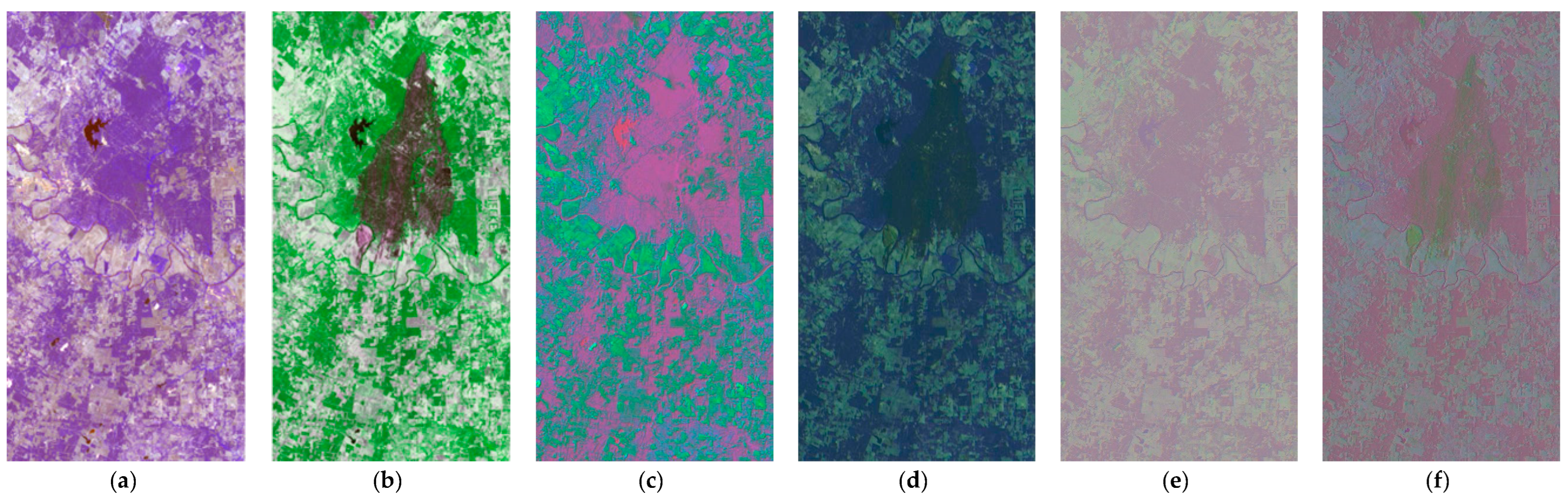
Figure 17.
Feature visualization of attention mechanisms in Forest fire in Texas dataset. (a) . (b) . (c) The output feature of ’s attention module. (d) The output feature of ’s attention module. (e) The output feature of ’s attention module. (f) The output feature of ’s attention module.
Figure 17.
Feature visualization of attention mechanisms in Forest fire in Texas dataset. (a) . (b) . (c) The output feature of ’s attention module. (d) The output feature of ’s attention module. (e) The output feature of ’s attention module. (f) The output feature of ’s attention module.

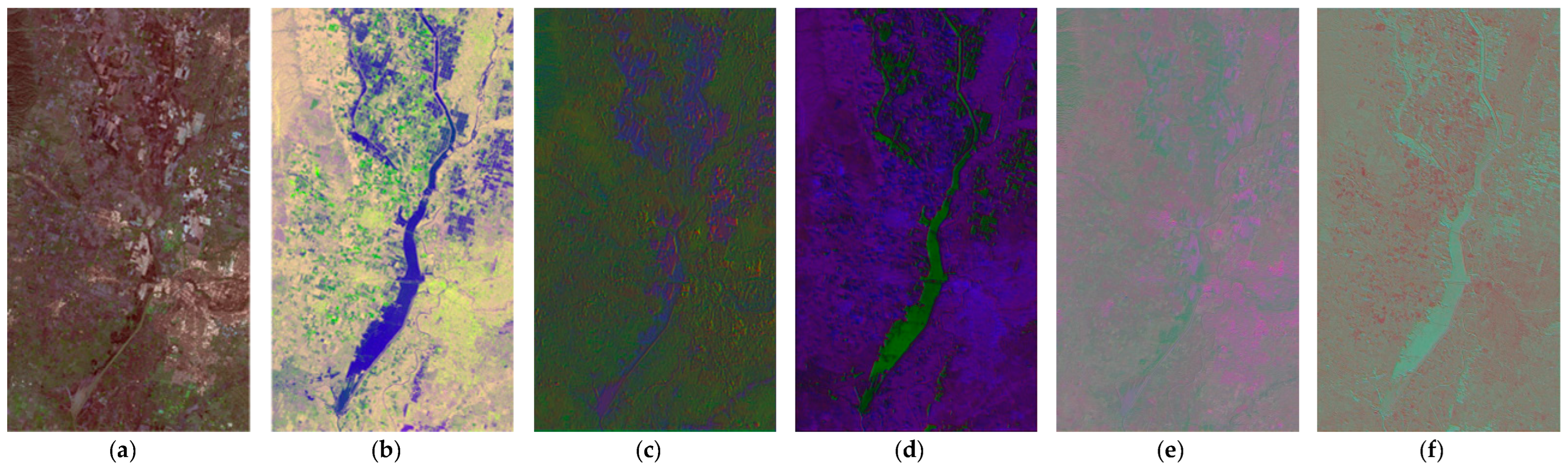
Figure 18.
Feature visualization of attention mechanisms in Flood in California dataset. (a) . (b) . (c) The output feature of ’s attention module. (d) The output feature of ’s attention module. (e) The output feature of ’s attention module. (f) The output feature of ’s attention module.
Figure 18.
Feature visualization of attention mechanisms in Flood in California dataset. (a) . (b) . (c) The output feature of ’s attention module. (d) The output feature of ’s attention module. (e) The output feature of ’s attention module. (f) The output feature of ’s attention module.

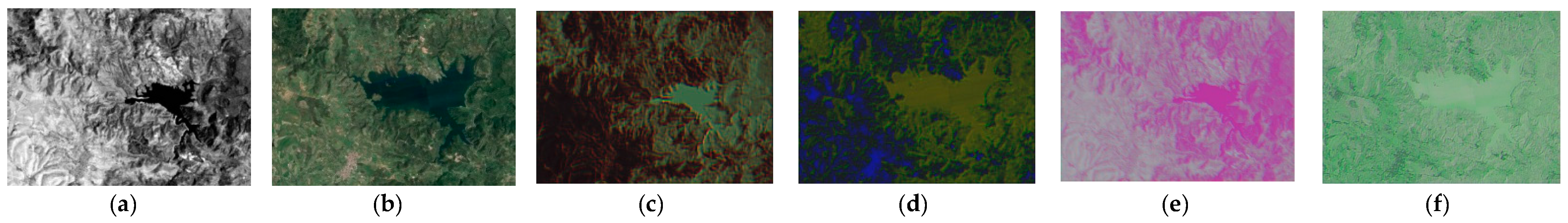
Figure 19.
Feature visualization of attention mechanisms in Lake overflow in Italy dataset. (a) . (b) . (c) The output feature of ’s attention module. (d) The output feature of ’s attention module. (e) The output feature of ’s attention module. (f) The output feature of ’s attention module.
Figure 19.
Feature visualization of attention mechanisms in Lake overflow in Italy dataset. (a) . (b) . (c) The output feature of ’s attention module. (d) The output feature of ’s attention module. (e) The output feature of ’s attention module. (f) The output feature of ’s attention module.

Figure 20.
Feature visualization of the proposed method and original neural network in Forest fire in Texas dataset. (a) . (b) . (c) The output feature of ’s attention module in the proposed method. (d) The output feature of ’s attention module in the proposed method. (e) The output feature of in the original neural network. (f) The output feature of in the original neural network.

Figure 21.
Feature visualization of the proposed method and original neural network in Flood in California dataset. (a) . (b) . (c) The output feature of ’s attention module in the proposed method. (d) The output feature of ’s attention module in the proposed method. (e) The output feature of in the original neural network. (f) The output feature of in the original neural network.

Figure 22.
Feature visualization of the proposed method and original neural network in Lake overflow in Italy dataset. (a) . (b) . (c) The output feature of ’s attention module in the proposed method. (d) The output feature of ’s attention module in the proposed method. (e) The output feature of in the original neural network. (f) The output feature of in the original neural network.


Table 1.
Objective evaluation indicators of the Forest fire in Texas dataset under different algorithms.
Table 1.
Objective evaluation indicators of the Forest fire in Texas dataset under different algorithms.
| Algorithm | Forest Fire in Texas | ||||
|---|---|---|---|---|---|
| OA | Precision | Recall | F1-Score | Kappa | |
| ACE-Net | 0.948 | 0.813 | 0.662 | 0.730 | 0.701 |
| CAN | 0.929 | 0.726 | 0.533 | 0.615 | 0.576 |
| SCCN | 0.928 | 0.604 | 0.935 | 0.734 | 0.694 |
| NPSG | 0.895 | 0.504 | 0.982 | 0.666 | 0.612 |
| INLPG | 0.932 | 0.765 | 0.519 | 0.618 | 0.582 |
| CAA | 0.975 | 0.895 | 0.876 | 0.885 | 0.871 |
| TSCNet | 0.976 | 0.908 | 0.852 | 0.879 | 0.873 |
Table 2.
Objective evaluation indicators of the Flood in California dataset under different algorithms.
Table 2.
Objective evaluation indicators of the Flood in California dataset under different algorithms.
| Algorithm | Flood in California | ||||
|---|---|---|---|---|---|
| OA | Precision | Recall | F1-Score | Kappa | |
| ACE-Net | 0.919 | 0.455 | 0.515 | 0.483 | 0.437 |
| CAN | 0.925 | 0.463 | 0.351 | 0.400 | 0.362 |
| SCCN | 0.903 | 0.435 | 0.675 | 0.529 | 0.448 |
| NPSG | 0.924 | 0.496 | 0.480 | 0.488 | 0.429 |
| INLPG | 0.931 | 0.547 | 0.568 | 0.557 | 0.500 |
| CAA | 0.923 | 0.537 | 0.560 | 0.548 | 0.506 |
| TSCNet | 0.939 | 0.686 | 0.494 | 0.574 | 0.542 |
Table 3.
Objective evaluation indicators of the Lake overflow in Italy dataset under different algorithms.
Table 3.
Objective evaluation indicators of the Lake overflow in Italy dataset under different algorithms.
| Algorithm | Lake Overflow in Italy | ||||
|---|---|---|---|---|---|
| OA | Precision | Recall | F1-Score | Kappa | |
| ACE-Net | 0.902 | 0.328 | 0.554 | 0.412 | 0.362 |
| CAN | 0.929 | 0.429 | 0.448 | 0.439 | 0.401 |
| SCCN | 0.892 | 0.333 | 0.754 | 0.462 | 0.412 |
| NPSG | 0.947 | 0.563 | 0.614 | 0.587 | 0.559 |
| INLPG | 0.918 | 0.415 | 0.796 | 0.546 | 0.506 |
| CAA | 0.949 | 0.563 | 0.792 | 0.658 | 0.631 |
| TSCNet | 0.955 | 0.595 | 0.782 | 0.676 | 0.654 |
Table 4.
Comparison of wavelet and attention module on three datasets.
| Method | Forest Fire in Texas | Flood in California | Lake Overflow in Italy | |||
|---|---|---|---|---|---|---|
| OA | Kappa | OA | Kappa | OA | Kappa | |
| None | 0.961 | 0.781 | 0.919 | 0.455 | 0.914 | 0.434 |
| Wavelet | 0.971 | 0.838 | 0.933 | 0.504 | 0.949 | 0.622 |
| Attention | 0.966 | 0.810 | 0.928 | 0.500 | 0.921 | 0.468 |
| Wavelet+Attention | 0.976 | 0.873 | 0.939 | 0.542 | 0.955 | 0.654 |
Table 5.
Comparison of single attention module on three datasets.
| Method | Forest Fire in Texas | Flood in California | Lake Overflow in Italy | |||
|---|---|---|---|---|---|---|
| OA | Kappa | OA | Kappa | OA | Kappa | |
| Wavelet + Channel Attention | 0.966 | 0.812 | 0.932 | 0.492 | 0.951 | 0.627 |
| Wavelet + Spatial Attention | 0.972 | 0.845 | 0.932 | 0.490 | 0.954 | 0.651 |
| Wavelet + Attention | 0.976 | 0.873 | 0.939 | 0.542 | 0.955 | 0.654 |
Disclaimer/Publisher’s Note: The statements, opinions and data contained in all publications are solely those of the individual author(s) and contributor(s) and not of MDPI and/or the editor(s). MDPI and/or the editor(s) disclaim responsibility for any injury to people or property resulting from any ideas, methods, instructions or products referred to in the content. |
© 2023 by the authors. Licensee MDPI, Basel, Switzerland. This article is an open access article distributed under the terms and conditions of the Creative Commons Attribution (CC BY) license (https://creativecommons.org/licenses/by/4.0/).
Share and Cite
MDPI and ACS Style
Wang, X.; Cheng, W.; Feng, Y.; Song, R. TSCNet: Topological Structure Coupling Network for Change Detection of Heterogeneous Remote Sensing Images. Remote Sens. 2023, 15, 621. https://0-doi-org.brum.beds.ac.uk/10.3390/rs15030621
AMA Style
Wang X, Cheng W, Feng Y, Song R. TSCNet: Topological Structure Coupling Network for Change Detection of Heterogeneous Remote Sensing Images. Remote Sensing. 2023; 15(3):621. https://0-doi-org.brum.beds.ac.uk/10.3390/rs15030621
Chicago/Turabian StyleWang, Xianghai, Wei Cheng, Yining Feng, and Ruoxi Song. 2023. "TSCNet: Topological Structure Coupling Network for Change Detection of Heterogeneous Remote Sensing Images" Remote Sensing 15, no. 3: 621. https://0-doi-org.brum.beds.ac.uk/10.3390/rs15030621
Note that from the first issue of 2016, this journal uses article numbers instead of page numbers. See further details here.