Article

Volcanic Cloud Detection and Retrieval Using Satellite Multisensor Observations

1
Dipartimento di Ingegneria dell’Informazione, Elettronica e Telecomunicazioni, Sapienza Università di Roma, 00185 Roma, Italy
2
Istituto Nazionale di Geofisica e Vulcanologia, 40128 Bologna, Italy
3
Centre of Excellence CETEMPS, University of L’Aquila, 67100 L’Aquila, Italy
4
Istituto Nazionale di Geofisica e Vulcanologia, Osservatorio Etneo, 95100 Catania, Italy
5
Istituto Nazionale di Geofisica e Vulcanologia, ONT, 00143 Roma, Italy
*
Author to whom correspondence should be addressed.
Submission received: 12 December 2022 / Revised: 30 January 2023 / Accepted: 2 February 2023 / Published: 5 February 2023
(This article belongs to the Special Issue Assessment and Prediction of Volcano Hazard Using Remote Sensing)

Abstract

:
Satellite microwave (MW) and millimetre-wave (MMW) passive sensors can be used to detect volcanic clouds because of their sensitivity to larger volcanic particles (i.e., size bigger than 20 µm). In this work, we combine the MW-MMW observations with thermal-infrared (TIR) radiometric data from the Low Earth Orbit (LEO) spectroradiometer to have a complete characterisation of volcanic plumes. We describe new physical-statistical methods, which combine machine learning techniques, aimed at detecting and retrieving volcanic clouds of two highly explosive eruptions: the 2014 Kelud and 2015 Calbuco test cases. For the detection procedure, we compare the well-known split-window methods with a machine learning algorithm named random forest (RF). Our work highlights how the machine learning method is suitable to detect volcanic clouds using different spectral signatures without fixing a threshold. Moreover, the RF model allows images to be automatically processed with promising results (90% of the area correctly identified). For the retrieval procedure of the mass of volcanic particles, we consider two methods, one based on the maximum likelihood estimation (MLE) and one using the neural network (NN) architecture. Results show a good comparison of the mass obtained using the MLE and NN methods for all the analysed bands. Summing the MW-MMW and TIR estimates, we obtain the following masses: 1.11 ± 0.40 × 10¹¹ kg (MLE method) and 1.32 ± 0.47 × 10¹¹ kg (NN method) for Kelud; 4.48 ± 1.61 × 10¹⁰ kg (MLE method) and 4.32 ± 1.56 × 10¹⁰ kg (NN method) for Calbuco. This work shows how machine learning techniques can be an effective tool for volcanic cloud detection and how the synergic use of the TIR and MW-MMW observations can give more accurate estimates of the near-source volcanic clouds.

1. Introduction

Volcanic eruptions are one of the most impressive and dangerous natural phenomena on our planet that, over the years, have influenced human life. During highly explosive eruptions, a great number of volcanic particles, also named tephra, are ejected into the atmosphere, and can remain suspended for several weeks. The surrounding areas of volcanoes are highly exposed to major hazards due to the fall out of blocks/bombs (size > 32 mm) and lapilli (size > 2 mm) [1,2]. Smaller particles (coarse ash < 2 mm and fine ash < 63 μm), instead, can travel for long distances in a few hours and remain suspended in the atmosphere for days. These smaller particles are largely responsible for damaging aircrafts and creating aviation traffic impairments [3]. For this reason, timely predictions of time–space dispersion of volcanic particles can ensure an improvement in defining the golden standard for airline flights and prevent damages [1]. Orbiting satellite observations can provide a large amount of daily data. The global perspective offered by Geosynchronous Earth Orbit (GEO) and the Low Earth Orbit (LEO) satellite systems is of vital importance for monitoring volcanoes [4,5], especially those in remote and inaccessible areas. Data from the LEO satellite microwave and millimetre-wave (MW-MMW) radiometers, such as Advanced Technology Microwave Sounder (ATMS) and Microwave Humidity Sounder (MHS), can be combined with thermal-infrared (TIR) spectroradiometers, such as Visible Infrared Imaging Radiometer Suite (VIIRS) and Advanced Very High Resolution Radiometer (AVHRR), to have more accurate estimates of the near-source volcanic cloud [1]. Whereas the LEO infrared data analysis represents the classic approach in the study of explosive activity by satellite, given their remarkable spatial resolution and sensitivity to ash clouds, their brightness temperature (BT) difference signatures can saturate because of large amounts of tephra mass mainly near the volcanic source. Moreover, the presence of tephra with a radius larger than 15 µm cannot be detected using these sensors, due to their detection limits [1,6], leading to inaccurate detections of some properties in the proximal or near-source volcanic cloud. In support of the TIR sensors, the MW-MMW sensors allow larger volcanic particles (⪆50 µm) to be observed. Actually, the near-source volcanic plume does not typically extinguish the MW-MMW signal, especially in the first hours of the eruptive event [1], probing the entire eruption column [7]. However, one of the drawbacks of MW-MMW sensors is the poor spatial resolution (up to 32 km). In the past, the MW-MMW bands have also been exploited to study volcanic plumes and their electrification processes [8,9,10].
The goal of this paper is to show how the analysis of both MW-MMW and TIR spectral signatures improves the characterisation of the volcanic plume in terms of detection and mass retrieval. For the detection, we worked in a statistical learning framework to develop a model capable of automatically processing images without the arbitrary threshold choice. In terms of retrieval, the new developed radiative transfer model algorithm (RTMA) is used to estimate the total columnar content (TCC) and, in turn, the mass for both MW-MMW and TIR. In this respect, two minimisation techniques, the MLE [11,12,13] and the NN [14,15,16], are also compared and discussed. The paper is structured as follows: Section 2 introduces the satellite sensors, the detection methods, the RTMA and the retrieval methods; Section 3 illustrates the 2014 Kelud and the 2015 Calbuco eruptions with an explorative data analysis of the satellite products; Section 4 shows the detection and retrieval results in two subsections, one per each eruption; Section 5 discusses the results and addresses future developments.

2. Methods

This section is divided into four subsections; the first describes the considered sensors for the analysis, the second discusses the split-window and the RF detection methods, the third describes the RTMA and the fourth focuses on the empirical approach.

2.1. Satellite Data

For the purpose of this work, we observed volcanic plumes using data coming from the ATMS and VIIRS, both on board the Suomi-National Polar-orbiting Partnership (S-NPP) LEO weather satellite provided by National Oceanic and Atmospheric Administration (NOAA) (all the acronyms are in Glossary). The ATMS sensor is a passive cross-track total power MW radiometer that measures microwave energy emitted and scattered by the atmosphere. It provides daily global atmospheric temperature, moisture and pressure profiles. It collects information in the frequency window from 23.80 to 183.31 GHz. This window is divided into 22 channels, with channels 1-2-16 detecting quasi-vertical polarisation, while the other 19 quasi-horizontal polarisation [17,18,19]. The spatial resolution is 16 km for the channels from 165.50 to 183.31 GHz, 32 km for the channels from 50.30 to 88.20 GHz and 75 km for the channels from 23.80 and 31.40 GHz. The VIIRS instrument is a whiskbroom scanning radiometer with an angular field of view of 112.56° in the cross-track direction and a swath width of 3000 km. It acquires information in 22 spectral bands from 0.412 to 12.01 μm. The measured spectrum range is divided into 16 moderate resolution bands with 750 m spatial resolution, 5 imaging resolution bands with 375 m spatial resolution, and 1 panchromatic day/night band with a spatial resolution of 375 m [20,21]. The level 1B products used in this work were downloaded from https://www.avl.class.noaa.gov/saa/products/welcome (accessed on 12 December 2022) for ATMS and VIIRS sensors and from https://eoportal.eumetsat.int/userMgmt/confirmed.faces (accessed on 12 December 2022) for MHS and AVHRR sensors [22,23]. The MHS and the AVHRR sensors were used only to train the RF model. The scripts used for the analyses were coded in Matlab and Python. Finally, the colour map plots were generated using the “colorcet” library, which is a collection of perceptually uniform colour maps (https://colorcet.com/index.html, accessed on 12 December 2022).

2.2. Volcanic Cloud Detection

In this subsection, we focus on the detection of volcanic clouds. We first present the multi-spectral brightness temperature difference (or split-window) method (see Section 2.2.1) and then the RF method (see Section 2.2.2).

2.2.1. Multi-Spectral Brightness Temperature Difference

Volcanic clouds in the infrared spectrum can be identified by selecting pixels with a brightness temperature difference (BTD) below a fixed threshold ( t B T D ) [24,25,26]:
B T D = B T 10.8 μ m B T 12 μ m < t B T D
A good approach is to apply different thresholds and see which one is most likely to represent the eruption [26,27]. The style of the eruption and the different weather conditions may have an influence on the threshold values. The higher the threshold, the higher the chance of having false alarms (i.e., t B T D ~ 0 K). In contrast, a lower threshold (i.e., < 0 K) increases the chance of underestimating the ash-contaminated areas. In terms of BTD thresholds, we use −0.2 K and −1.5 K for Kelud and Calbuco eruptions, respectively.
Since the clouds are located at high altitudes, they appear cold while observed at frequencies above 100 GHz [28]. When working at higher frequencies (>100 GHz), bare soil and oceans present higher BTs compared to the clouds’ BTs. The identification of the volcanic cloud in the MW-MMW is a two-step identification method called microwave spectral difference (MSD). The first step is called the microwave spectral difference window (MSDW) [29]:
M S D W = B T f w 1 B T f w 2
where f w 1 and f w 2 are two frequencies. The former is in the range 155–165 GHz, the latter in the range 85–95 GHz. For the ATMS sensor, f w 1 = 165.50 GHz and f w 2 = 88.20 GHz. All MSDW pixels, which are below a given threshold, are detected as clouds. By convention, this threshold is set equal to 0 K [29]. Once all the cloud pixels are detected, the second step separates meteorological from volcanic clouds [1,29]. Meteorological clouds are characterised by a marked amount of water, which makes the channel around 183.31 GHz more sensitive due to the presence of the water vapour absorption peak. Volcanic clouds, on the other hand, respond better at lower frequencies. The formula below implements the microwave spectral difference absorption (MSDA), the second step of the MSD method:
M S D A = B T f w 3 B T f w 1
where f w 1 and f w 3 are two different frequencies. For ATMS sensor f w 3 = 183.31 ± 3 GHz and f w 1 = 165.50 GHz. Volcanic plumes are separated from meteorological clouds by selecting the MSDA values below an arbitrary threshold, which is, by convention, set equal to 0 K [29]. False alarms can still occur also in this case. If the scene is mostly cloudy, fixing a threshold close to zero can increase the chance of having false alarms. Moreover, if scattered pixels are identified in the scene, these are excluded from the identification, since most aggregated pixels are more likely to belong to a proximal volcanic cloud [29]. In this way, only the most aggregated pixels are considered. In our analysis: the MSDW threshold is set to −9 K for Kelud eruption and to 0 K for Calbuco eruption; the MSDA threshold is set to 0 K for both eruptions. To summarise, it is not possible to assess that a given threshold can be useful to detect different volcanic clouds or even the same cloud at different instants mainly due to a change in the particle composition or different weather conditions, different times and different sensor settings [29,30].

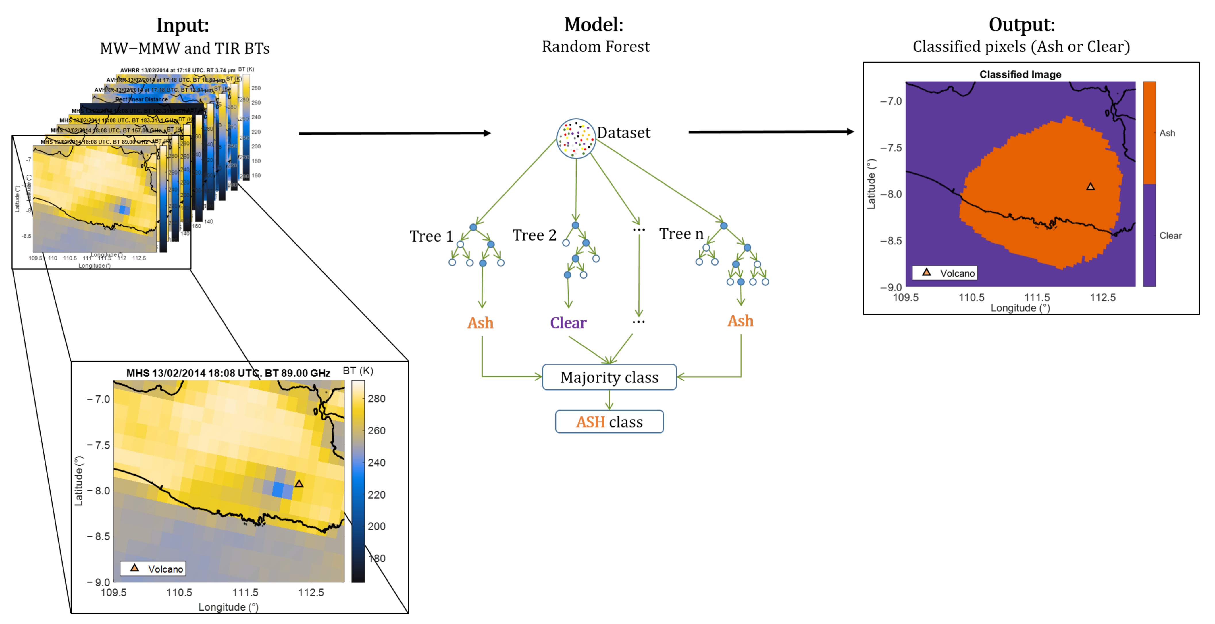
2.2.2. Random Forest Classification Technique

In the last decade, the use of machine learning algorithms became popular also in atmospheric science. Most of the works present in the literature use the collected radiances only in the infrared to make the detection [31,32,33]. In addition, most of these models are designed to work with one specific sensor, even if some new studies are developing sensor-independent schemes [34]. The presented model instead combines different spectral information (i.e., MW-MMW and TIR) to attempt a general rule applicable on different sensors onboard of different platforms. The goal is to find a model that can detect the volcanic cloud automatically (i.e., without user action) and independently from the used sensor. The learned model is obtained by the following procedure: (1) definition of training images; (2) identification of the most relevant features, i.e., those that can better reflect the variability of the dependent variable; (3) model training; (4) model performance and selection; (5) classification of unseen images. The training data sample uses data collected by the MW-MMW and TIR sensors for the 2014 Kelud and 2015 Calbuco eruptions. Table 1 summarises the data and their application in the RF classification.
The considered features are the common channels between the MHS-ATMS and AVHRR-VIIRS sensors plus the rectilinear distance (the sum of the absolute differences of the pixels’ Cartesian co-ordinates) of each pixel from the volcano. More specifically, we use the channels 88.20 GHz (89.00 GHz for MHS), 165.50 GHz (157.00 GHz for MHS), 183.31 ± 1 GHz, 183.31 ± 3 GHz, 12.01 μm, 10.80 μm and 3.70 μm (3.74 μm for AVHRR). Each pixel is then treated as an independent sample during the training process. Due to the sensors’ different pixel sizes, the MW-MMW observations were resampled on the TIR grid. In this way, each area is represented by the same number of pixels. The collected data are divided into sets, henceforth, train (80% of the pixels) and test (20% of the pixels) sets. The former is used to fit the model. The test is instead used to provide an unbiased evaluation of the model. The stratified cross-validation (CV) method was used to evaluate the actual model performance. With this method, we divide the training dataset into K-folds (i.e., different k datasets of equal sizes where the percentage of each class does not change in each fold). On each iteration, a kth dataset is used as a validation set and the remaining k-1 folds are used as training sets. The error is calculated on the held-out fold (i.e., the kth set). This process continues up until all the k folds (10 in total) are used as validation sets. The k-fold CV result is computed by averaging all the validation errors [35]. During the training process, different bagging and boosting tree-based algorithms with different configurations are considered. All the different learned models are compared with each other by using the averaged CV score to find the one that better captures the underlying distribution. The F1 score is used as the evaluation metric:
F 1 = 2 × ( P r e c i s i o n × R e c a l l ) ( P r e c i s i o n + R e c a l l )
The F1 score allows false alarms and false negatives (FN) to be balanced and can be considered as the harmonic mean of the recall and the precision scores, assuming values between 0 and 1 [35]. The precision is computed as TP/(TP + FP) and the recall as TP/(TP + FN), where TP is the true positives and FP is the false positives. The precision measures the model capability of mislabelling as positive a negative pixel; the recall measures the model capability to correctly classify the positive pixels. The best considered model is the one learned by the RF algorithm with an F1 CV score of 0.8900 and of 0.9000 on our test. The RF configuration is summarised as follows: N° estimators, that is the number of trees in the forest, is set equal to 25; Criterion, which controls the function used to measure the quality of each split in each tree, uses the Gini index; Max depth, which controls the depth of the trees (i.e., how many splits in total), is set equal to 6; Max features defines how many features are considered when defining the best split and it is set equal to log 2 ( N °   features ) ; Class weight is used to associate weights to each class considering the class frequency and it is set equal to balanced; Bootstrap is set equal to true. The output of the model is a 0–1 binary mask, 0 for clear pixels (coloured in purple) and 1 for contaminated tephra pixels (coloured in orange). Once the mask is generated, we apply a nearest neighbourhood approach to identify and then exclude small clusters far from the volcanic crater. For the RF algorithm, we use the scikit-learn library version 1.0.2 (https://scikit-learn.org/stable/, accessed on 12 December 2022) and Python 3.7 version [36,37,38]. A schematic representation of the classification methodology is displayed in Figure 1.

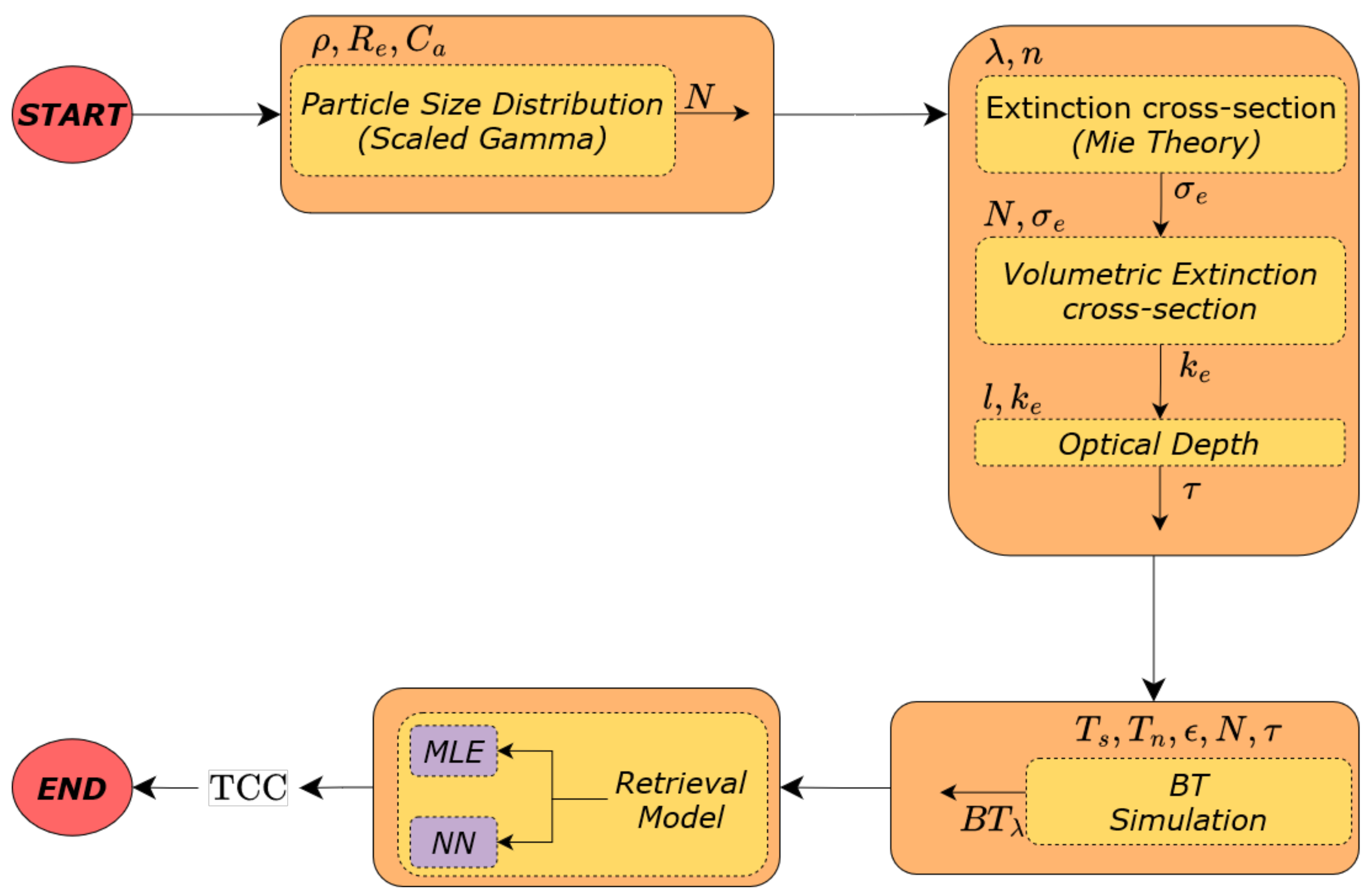
2.3. Radiative Transfer Modelling

The radiative transfer model (RTM) scheme is designed to simulate the BTs observed by the TIR and MW-MMW sensors (Figure 2). The contributions coming to the sensor are the background radiance (land or water), the atmosphere radiance and the space radiance (which is neglected during cloud physical properties retrieval [30]). We solve the radiative transfer differential equation by considering one- and two-layer approximations, with a normal pointing to the surface (i.e., we do not consider the inclination angle). We ignore the multiple scattering effect and the additional extension due to the electrostatic charge within highly explosive activity [39]. The one-layer model ( B T 1 L ) is applied to the TIR observations, as proposed in [24], whereas the two-layer model ( B T 2 L ) is applied to the MW-MMW observations. The B T 1 L (Figure 2 left panel) is the solution to the radiative transfer differential equation considering the one-layer approximation, where, T S and T C are, respectively, the surface and the top cloud temperature and e τ is the transmittance, expressed as a function of the optical depth τ, which is computed applying the following approximated formula:
τ = k e ( r ) l
where l is the geometric thickness of the cloud [24] and k e is the extinction coefficient, which is a function of the particle radius. The B T 2 L (Figure 2 right panel) represents the solution to the radiative transfer differential equation considering the two-layer approximation. The contributions coming to the sensor are the B T s u r f , which is the surface contribution that is irradiated upward to the satellite and takes into account the surface temperature, the ground emissivity and the transmittance of the two layers; the B T 1 u p , which is the first-layer brightness temperature that is irradiated upward; B T 1 d o w n , which is the first-layer brightness temperature that is first reflected and then irradiated upward to the sensor; the B T 2 d o w n , which is the second-layer brightness temperature that is first pushed downward and then it is irradiated upward to the sensor; and the B T 2 u p is the second-layer brightness temperature that is irradiated upward. T Z is the average temperature between T C and T S . T 1 and T 2 are the temperature of first and second layers, respectively, and Δ H , Δ H 1 and Δ H 2 are the respective layer heights.
The analysis in the remote sensing framework is solved by inverting the forward problem. The forward problem starts from volcanic cloud properties based on the literature (e.g., particle size, density and concentration [2]), and then computes synthetic BT measurements. The synthetic BTs are then compared with the observed BTs to retrieve the main features of volcanic clouds. Our R T M A can be summarised into four main blocks; in the first block, we obtain the particle size distribution, in our case, a scaled Gamma. The second block estimates the cloud physical properties and the third block simulates the BTs considering the previously estimated layer features. Finally, the fourth block uses both the MLE and NN methods to estimate the total columnar content (TCC). We consider volcanic plumes composed by particles having particle density (ρ), effective radius ( R e ) and concentration ( C a ) . Effective radius ( R e ) and concentration ( C a ) values vary depending on particle classes. In this case, a positive relation is considered, i.e., larger particles correspond to larger concentration, as expressed in [2]. For the MW-MMW, we use the following classification: small lapilli (SL) having a particle density of 1200 kg/m3, R e in the interval 256–2048 μm and C a in the interval 103–2 × 10³ mg/m3 [2,40]. For the TIR, instead, we consider the class fine ash (FA) with the following characteristics: particle density of 2600 kg/m3, R e in the interval 0.07–10.00 μm and C a in the interval 100–101.5 mg/m3 [2]. The complex refractive index (n) is called by the second block when cloud properties are retrieved. For MW-MMW, we use n a s h = 2.48 − i0.016 [40]. In the case of TIR, the refractive index and the extinction coefficient are derived by analysing results contained at Aerosol Refractive Index Archive (ARIA, University of Oxford, http://eodg.atm.ox.ac.uk/ARIA/, accessed on 12 December 2022). The used refractive indexes at 10.80 and 12.00 μm are, respectively, 2.10 + i0.41 and 1.79 + i0.19 for Kelud and 2.435 + i1.079 and 2.084 + i0.197 for Calbuco. The scattering of these particles is well described by Mie scattering theory. The volumetric extinction cross-section k e is calculated by considering the extinction cross-section ( σ e ) and the particle distribution N(r) [41,42]:
k e ( r ) = r m i n r m a x σ e N ( r ) d ( r )                                                               ( m 1 )
where the extinction cross-section σ e is calculated as:
σ e = σ s + σ a = W e P i                                                                               ( m 2 )
with W e as the total extinction power, P i the incoming incident power density, σ a the absorption cross-section coefficient and σ s the scattering cross-section coefficient [41,42]. The particle size distribution N(r) is computed as:
N ( r ) = N n p ( 6 ( 3.67 + μ ) μ + 4 3.67 4 Γ ( μ + 4 ) ) ( 2 r 2 r n p ) μ e ( 3.67 + μ ) ( 2 r 2 r n p )                     ( m 4 )
where N n p is the intercept parameter, 2 r n p is the volume-weighted median diameter and μ is the shape parameter of the gamma distribution [40]. The surface and the cloud temperatures, called by the fourth block, are used to compute the synthetic BTs with the surface emissivity set to 0.90 for MW-MMW [29]. The well-known radiative transfer differential equation is solved by considering the one- and two-layer approximations [41,42]:
B T H = B T 0 e τ ( 0 , H ) + 0 H α ν ( 1 ω ) ϵ T e τ ( s , H ) d s                                         ( K )
where α ν is the absorption coefficient, ω is the albedo, ϵ is the emissivity,   τ ( 0 , H ) and τ ( s , H ) are, respectively, the entire atmosphere optical thickness and the optical thickness from layer s to the top of the atmosphere, B T 0 is the surface temperature and T is the physical temperature of the medium. Figure 3 shows the block diagram of the developed R T M A .
Figure 4 shows the solution of the R T M A plotted in arch curves. For both MW-MMW and TIR curves, we return the associated effective radius. For MW-MMW we show the effective radius interval that goes from 0.28 to 2.00 mm. Instead, for TIR measurements, we show the effective radius interval from 1.50 to 10.00 μm.
The TCC or mass loading identifies the superficial density of the volcanic cloud. For that purpose, the cloud is treated as a cylinder and the TCC is computed by the integral of the ash content into a cylinder of unit area as [24,25]:
T C C = 4 3 π H r m i n r m a x ρ ( r ) r 3 N ( r ) d r                                         ( kg m 2 )
where ρ ( r ) is the ash cloud density, r is the particle radius and H is the height. The total mass is then estimated by multiplying (10) for the area of each pixel and aggregating them. The pixel area is calculated from the image itself by looking at the latitude and longitude information. This allows a higher level of flexibility since the estimate is independent from the sensor and the scanning angle. The uncertainty related to the TCC estimate is given by:
ε T C C = δ T C C T C C = ( δ H H ) 2 + ( δ r r ) 2
where we assume the following values for each independent parameter: δr = 0.20r and δH = 0.30H. The relative percentage error ε T C C is equal to 36%. For each simulated BT, different information is known, such as R e , C a and τ . For observed pixels these quantities are retrieved by associating each of them to their closest curves. In this work, we compare two methods to pair synthetic BTs with observed BTs: the maximum a posteriori probability (MAP) and an NN architecture. Assuming uniform prior information, the MAP and the MLE converge to the same solution. Moreover, assuming Gaussian-likelihood statistics of the difference between the synthetic BTs and observed BTs and uncorrelation between the deviations (i.e., errors) of the same observables, the MLE reduces to the minimisation of a quadratic form [2]. The MLE method is used to retrieve information about R e and TCC, computed by the R T M A , for the collected BTs.
The NN architectures are particularly powerful to solve nonlinear problems. In this work, we consider an architecture composed by one hidden layer. This configuration returns good results to solve this multiple-nonlinear regression problem. The NN fitting procedure is involved in defining the unknown parameters that fit the training data well. In NN, the unknown parameters are the weights θ. Since it is a regression problem, the root mean squared error (RMSE) is used as a measure of fit. The stochastic gradient descent optimisation method was used to minimise the mean squared error (MSE) loss function [14,35]. This speeds up the computation since the gradient is not computed on the whole dataset but on a randomly selected subset. More specifically, the adaptive moment estimation (ADAM) method is used [43]. The learning rate γ r for the batch size is optimised by a linear search that minimises the error function at each iteration. This means that γ r goes to zero while increasing the number of iterations r. ADAM uses the first and the second moments of the gradients to adaptively adjust the learning rate. The weights are randomly initialised with values near to zero. In this way, the model becomes nonlinear as soon as the weights are updated [14]. The response variables TCC and R e are dependent upon the BTs and upon each other. This requires a model which is able to predict both quantities at once. NN allows a multi-output model to be defined. For that reason, the NN architecture presents two nodes in the output layer, one per each response variable. The input layer, instead, is composed by n numbers of nodes based on the number of simulated BTs. Mathematically, the used architecture can be expressed as follows [14]:
f ( x ) = g ( W 2 a ( W 1 x + b 1 ) + b 2 )
where g is the output function, W i is the weight matrix i , a is the activation function, x is the input (simulated BTs) and b i the bias matrix i . The dataset used to train and evaluate the model is composed by the BTs simulated with the R T M A . In particular, for each simulated channel, there is a 500 × 500 matrix where each entrance is a simulated BT expressed in K. Then, the dataset is divided into train (80%) and test (20%) sets. The CV method, applied on the train set, was used to evaluate the actual NN performance by using the RMSE metric. The NN architecture is summarised in Figure 5.
Since we are working with both the MW-MMW and TIR sensors, we developed two NN models. The NN model for the MW-MMW observations has three input nodes represented by the synthetic BTs at frequencies 88.20, 165.50 and 183.31 GHz. The hidden layer is composed of 256 nodes. The batch size is set to 512. The number of epochs is set to a large number with the early stopping method. In this way, the training stops when the model performance stops, improving after a given number of iterations. The rectified linear unit (ReLu) activation function is used in the hidden layer [14,44,45]. The NN architecture for the TIR has instead two input nodes: BTs at 10.80 and 12.01 μm. The hidden layer is composed of 128 nodes. The batch size and number of epochs are treated as for the MW-MMW network. Moreover, here, the ReLu activation function is used in the hidden layer. For the NN implementation, we use the TensorFlow 2.8.2 open-source platform (https://github.com/tensorflow/tensorflow, accessed on 12 December 2022) and the Keras 2.8 deep learning API (https://github.com/keras-team/keras, accessed on 12 December 2022) written in Python [46].

2.4. The Empirical Parametric Retrieval (EPR) Method

The MW-MMW mass loading estimates, obtained with the MLE and NN methods, are compared with the parametric regressive formula named empirical parametric retrieval (EPR) [1]. The EPR is used as a quality measure of the MLE and NN estimates. The EPR comes from a regression analysis applied on a numerical model simulation in terms of MW BTs of volcanic plumes over land [1]:
L t = a t ( ρ ρ 0 ) + b t ( ρ ρ 0 ) B T f         ( kg m 2 )
where a t = 63.84, b t = −0.2564 and ρ = ρ 0 = 2500 kg/m3. The B T f is the brightness temperature around the 183 GHz channel, the frequency near the water vapour absorption peak. The tephra mass loading estimate ( L t ) is almost not dependent on the surface land emissivity variation due to the use of the absorption channel around 183 GHz [1].

3. Test Cases

In this section we describe the Kelud and Calbuco eruptions conjointly with an explorative data analysis of the ATMS and VIIRS products.

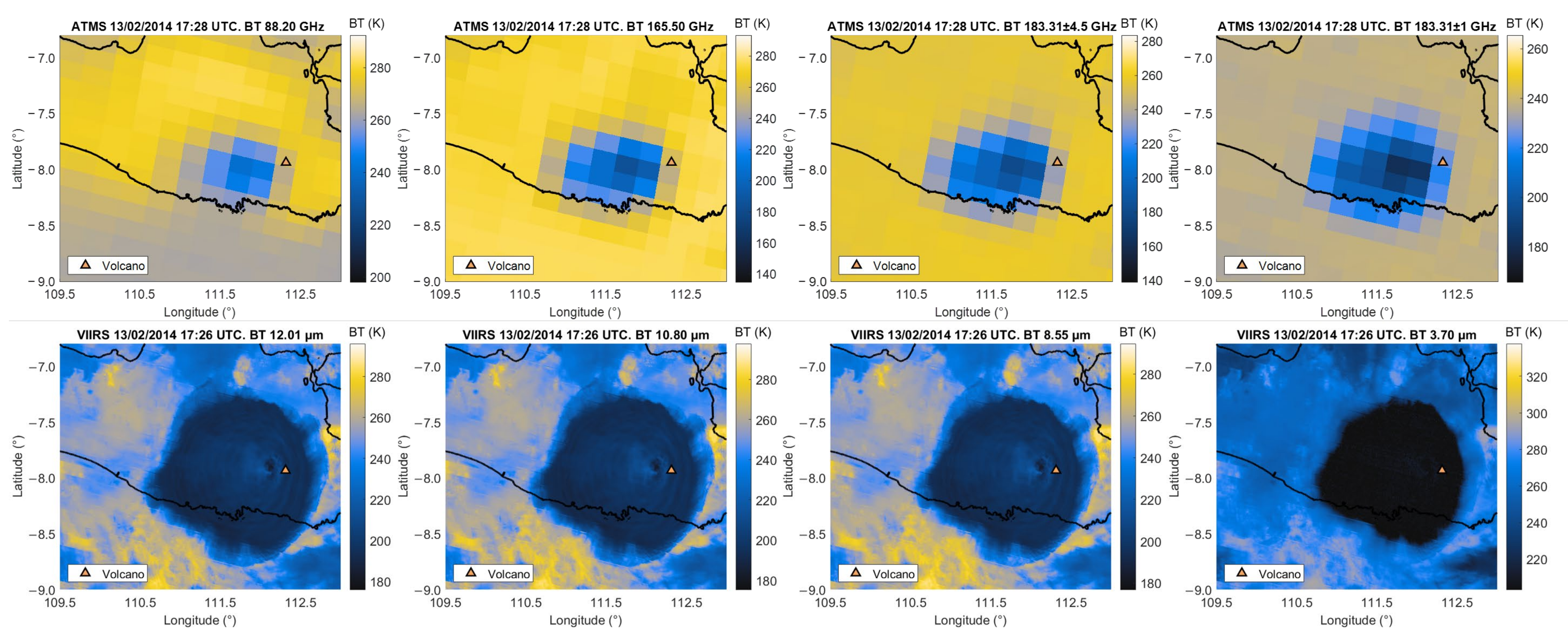
3.1. The Kelud Eruption in 2014

Kelud volcano is one of the most dangerous stratovolcanoes in Indonesia. It is located at −7°55′48.00″ S 112°18′28.80″ E, East Java. At the beginning of 2014, the earthquake activity started increasing, alerting the local community of an awakening of the volcano. On 13th February 2014 at 15:46 UTC, the seismic activity stopped, indicating the onset of the eruption. The first recorded explosion formed a high eruption column. The top of the umbrella cloud’s height was estimated at approximately 20 km, with a diameter of more than 200 km [47]. The plume drifted south-west across the Java Island and the Indian Ocean [48]. The eruption caused many problems to air traffic; indeed, many local flights were cancelled or rerouted. The tephra ashfall damaged schools, homes and local businesses. More than 76,000 people were evacuated from their homes until the eruption activity stopped on 17th February [47,48].
Figure 6 shows the explorative analysis from the ATMS and VIIRS sensors. The first row of Figure 6 shows the channels 88.20, 165.50, 183.31 ± 4.50 and 183.31 ± 1 GHz. Over the land, the use of frequencies above 80 GHz displays how the scattering is stronger if compared with the emission-based process. The background BT signatures at frequencies above 90 GHz appear to be hotter (yellow pixels) than the cloud ones (blue and dark blue pixels). This allows the visual detection of volcanic cloud pixels. The second row represents the channels 12.01, 10.80, 8.55 and 3.70 µm of the VIIRS sensor. The presence of meteorological clouds coupled with shorter wavelengths (compared to MW-MMW) does not allow full discrimination between the volcanic cloud and the background. Indeed, by looking only at channel 3.70 µm, both background and the contour of the cloud appear blue. The other TIR channels better distinguish the cloud and the background (yellow areas). However, the borders of the clouds are still not well separated by the meteorological clouds (light blue pixels around 240 K).

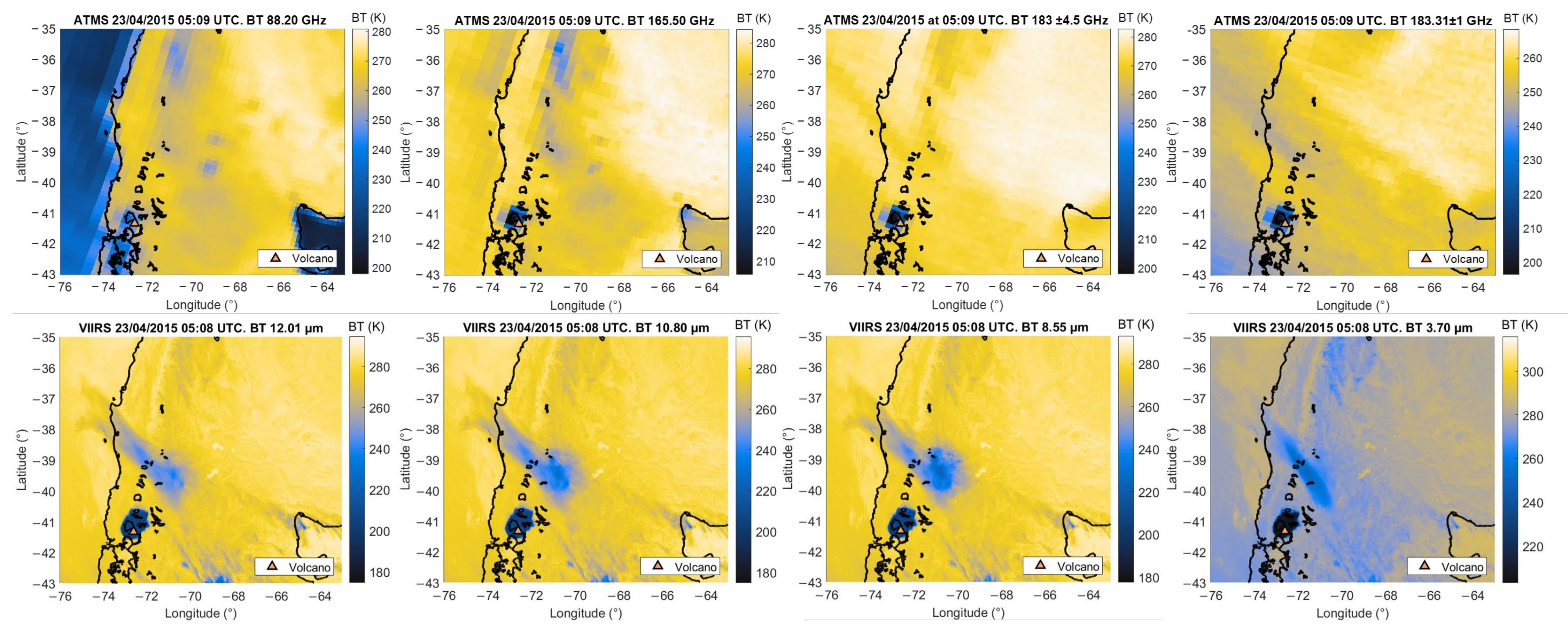
3.2. The Calbuco Eruption in 2015

Calbuco is an active and hazardous stratovolcano located at 41°20′ S–72°37′ W in southern Chile. It covers an area of 150 km2, with its summit at 2003 m above sea level. After 54 years of calm, it reawakened on 22 April 2015 at 21:08 UTC. Alarms of the volcano’s awakening were signalled by an intense seismic activity [49]. On 23 April 2015 at 04:00 UTC, a strong explosion occurred, which lasted about six hours. The ash plume, with a maximum estimated altitude of about 15–20 km, moved in the north-east direction [1]. On 24th April 2015 at 02:30 UTC, a smaller explosion occurred. During those events, different cities registered inconveniences and mobility problems. The air traffic in the airport of Puerto Montt was also suspended. Different cities and areas were affected by tephra fallout, such as Los Lagos, Los Rios and Araucani [1].
Figure 7 is an explorative analysis from the ATMS and VIIRS sensors. Moreover, in this case, the first row of the figure shows the channels 88.20, 165.50, 183.31 ± 4.50 and 183.31 ± 1 GHz. The volcanic cloud pixels appear colder while moving at frequencies above 90 GHz, due to the increasing ratio between particle sizes and wavelengths. In particular, frequencies around 165.50 GHz and 183.31 GHz allow a clear discrimination between the background and the volcanic cloud. The coldest pixels (i.e., darkest blue and black) highlight the area covered by the volcanic cloud, whereas yellow pixels the background. It is interesting to notice how, using the ATMS sensor, the distal cloud is not visible in any of these channels. This is because these frequencies are not sensitive to smaller dispersed ashes. The channels 12.01, 10.80 and 8.55 µm show in dark blue and black the near-source cloud, in light blue the dispersed cloud and in yellow the background. The channel 3.70 µm allows a good visual representation of the volcanic cloud at the source (darkest blue and black pixels) but, due to its sensitivity to finest particles, the volcanic distal cloud may be partially masked by the presence of the other background atmospheric effects.

4. Results

In this chapter, we show the detection and the retrieval using MW-MMW and TIR spectral signatures. We first describe the detection results obtained using the split window methods and the RF model, then the estimates obtained using the MLE and the NN methods. For the detection, the results are displayed with three images, where images A and B show the detection using the MSD and BTD methods, respectively; image C shows the detection using the RF model. For the RF outputs, the results are plotted using three different colours. Regarding the retrieval, we provide simulated arch curves, representing the simulated BTs, for both spectral signatures. The TCC maps are grouped into two figures composed of five panels each. Section 4.1 is dedicated to the Kelud event and Section 4.2 to the Calbuco event.

4.1. Kelud: Detection and Retrieval

For the Kelud eruption, the MSD cloud pixel identification is visible in Figure 8A. The M S D A is higher for pixels which are proximal to the volcanic crater. This effect is shown in this image by the pixels with the yellow shade colour (higher M S D A ) and dark blue pixels (smaller M S D A ). The BTD detection is displayed in Figure 8B. The reported values are already adjusted with the water vapour correction explained in Appendix A. The edges of the cloud are characterised by the presence of pixels with a BTD smaller than zero (pale-blue and light-yellow colours), whereas the pixels near the volcano are characterised by a BTD slightly above zero (yellow pixels), where the abundance of water particles is relevant. Figure 8C shows the output of the RF model. As a measure of comparison, the images A and B are overlapped and used as ground truth. In this way, every RF-classified pixel is compared with its symmetrical available in the A + B combined image. The pixel is coloured in purple if it is identified by both the methods, the MSD-BTD and the RF; it is magenta if it is identified by the RF but not by the MSD-BTD; it is orange if it is identified by the MSD-BTD but not by the RF. Almost 90% of the area is identified by the RF model (purple pixels). A small fraction is missing (i.e., orange pixels) and another small part disagrees with the MSD-BTD detection (magenta pixels). The overall F1 score on this image is 0.9049, which is a very high score and higher than the one obtained during the test phase, meaning that the model is performing correctly and it is not overfitting.
Regarding the retrieval, Figure 9A details the simulated curves for MW-MMW volcanic particles. The black points represent the volcanic particle pixels previously detected using the MSD method. These points are associated with particles of effective radius that vary from 0.28 to 0.60 mm. The points that lie outside the simulated curves are associated with their closest curve [24]. For the TIR curves, the detected ash particles have a particle radius that ranges between 5.00 and 10.00 μm. These points are represented in Figure 9B as orange points. The black points represent the MW-MMW-detected pixels, which were resampled on the TIR grid (this is the reason why there are more than those displayed in Figure 9A). As expected, many points lie outside the simulated curves and have a positive BTD. These are the points that represent the areas contaminated by particles not visible at the TIR wavelengths due to sensor detection limits.
Starting from these simulated curves, we perform the mass retrieval. Per each of the three methods, the MW-MMW masses are, respectively, EPR 1.54 ± 0.55 1011 kg, MLE 1.11 ± 0.40 × 10¹¹ kg and NN 1.30 ± 0.47 × 10¹¹ kg. All the three methods highlight how the higher masses are estimated to be in the centre of the cloud (yellow pixels of Figure 10A–C). The smaller masses are associated with the areas far away from the volcanic crater (blue pixels). The instantaneous total masses and the TCC maps, for both the MLE and the NN, are in good agreement with the one obtained using the parametric formula (EPR). Figure 10D,E show the estimated TCC maps for both MLE and NN methods considering TIR observations. The estimated masses are, respectively, MLE 2.25 ± 0.81 × 10⁹ kg and NN 2.16 ± 0.78 × 10⁹ kg. The MLE and the NN TIR results show the highest mass loading in the centre of the cloud (yellow pixels). However, the NN method shows a more homogeneous path in the map, with high mass loading areas also outside the centre of the cloud. This is more in line with the MW-MMW retrievals, in particular, the EPR (Figure 10A) and the NN (Figure 10C). Indeed, Figure 10A,C,E are in agreement with each other (see yellow and blue pixels) in terms of mapping. Then, the NN results (MW-MMW and TIR) better characterise the volcanic cloud. Moreover, our NN estimate of the mass, given by the sum of the MW-MMW and TIR estimates, is 1.32 ± 0.47 × 10¹¹ kg, which is in line (in terms of order of magnitude) with volcanological studies. Following [48,50], using field data collected on ground, a total erupted mass was estimated to be 3.30–6.60 × 10¹¹ kg. It is noteworthy that we are observing the eruption only at the time of the satellite overpass (17:28 UTC) when the eruption was still ongoing. This implies that we are not considering in the comparison the mass emitted after the satellite acquisition time until the end of the eruptive event.

4.2. Calbuco: Detection and Retrieval

For the Calbuco eruption, the MSD cloud pixel identification is displayed in Figure 11A. The M S D A assumes high values in almost the whole detected area, except for one pixel with a value of ≈−11 K. When the plume is spreading, it has a greater amount of fine particles, not detected by the MSD. The presence of smaller particles is, instead, well visible in Figure 11B (see outlines coloured in pale blue). As for Kelud, the reported BTDs values are already adjusted with the water vapour correction described in Appendix A. Figure 11C shows the output of the RF model. Moreover, here, the images A and B are overlapped and used as ground truth. Most of the pixels are coloured in purple, with an area coverage of about 90%. A small fraction is missing (i.e., orange pixels) and a very small fraction is wrongly classified (magenta pixels). The overall F1 score is 0.9271, which is even higher than the one obtained for the Kelud event (Figure 8C). This is because the fraction of false alarms is very small compared to the fraction visible in Figure 8C.
Figure 12 displays the R T M A results for both the MW-MMW and TIR sensors. Figure 12A displays the simulated arch curves for MW-MMW observations. The black points identify the detected MW-MMW pixels. The particle radius ranges in between 0.28 and 0.85 mm. For the TIR observations we show the results in Figure 12B. Moreover, here, the black points highlight the MW-MMW detected pixels which were resampled on the TIR grid. As expected, many of these points lie outside the simulated TIR curves. At the time of the pass of the Soumi-NPP satellite, the volcano was erupting for the second time. Indeed, the VIIRS sensor also detected a first event (22 April 2015 at 21:08 UTC) represented in Figure 12B by the yellow points. The orange points, instead, represent the pixels belonging to the near-source cloud (i.e., the second event at 05:09 UTC), the one detected also by the ATMS sensor. It is visible how the two events, observed in the TIR region, have particles with different sizes (from 2.00 to 4.00 μm for the first event and from 2.50 to 5.00 μm for the second event). The reason is that bigger particles remain suspended in atmosphere for less time due to their bigger mass.
Associating each observation to its closest curve, the retrieval is, hence, performed. The MW-MMW masses obtained with the considered methods are EPR 4.21 ± 1.51 × 10¹⁰ kg; MLE 4.33 ± 1.56 1010 kg; and NN 4.17 ± 1.50 × 10¹⁰ kg, respectively. For all three methods, the higher mass is estimated on the west side of the volcano (yellow pixels), in proximity to the top of the umbrella at an altitude of ≈19 km [1], see Figure 13A–C. The smaller mass is associated with the areas far from the volcanic crater (bright blue pixels). The estimated mass and the TCC maps, for both the MLE and the NN, are in good agreement with the one obtained using the parametric formula (EPR). The small changes between the estimates can be explained with the different polarisation corrections and the ignored multiple diffusion effects. For the TIR observations, the estimated masses are, respectively, MLE 1.48 ± 0.53 × 10⁹ kg and NN 1.54 ± 0.55 × 10⁹ kg. For consistency, we also report the estimates for the distal ash cloud, which are 2.37 ± 0.85 × 10⁹ kg for MLE and 2.17 ± 0.78 × 10⁹ kg for NN. The TIR proximal and distal masses are reported in Figure 13D,E with the acronyms M a s s P and M a s s D . For both MLE and NN TIR results, the highest mass loading is associated with the centre of the cloud (yellow pixels) with values in the range of 0.06–0.08 kg/m2, see Figure 13D,E. However, the NN TCC map (Figure 13E) is more in line with the EPR map (Figure 13A). Indeed, Figure 13A,C,E are in good agreement with each other (see yellow and blue pixels) in terms of mapping. Moreover, in this case, we conclude that the NN results are more in line with the EPR results and past studies [1,49]. If we sum the NN MW-MMW and TIR mass estimates, we obtain a mass of 4.32 ± 1.56 1010 kg that is in line with previous studies on the deposit (3.33–4.71 1010 kg) [49].

5. Conclusions

The aim of the work was to show the synergy given by the combination of the MW-MMW and TIR observations to study volcanic clouds. The application on the Kelud and Calbuco case studies highlighted how the combination of these two spectral signatures can increase the quality of the detection and the mass retrieval. The proposed methodologies allow the study of the time evolution in terms of scene coverage and mass of the volcanic cloud.
The RF model allows images to be automatically processed without the arbitrary threshold choice and has, in our opinion, promising results. Moreover, our results underline how it is possible to combine different spectral information, coming from different platforms, to have a better characterisation of the volcanic cloud. The RF model is able to balance false alarms and the FN while classifying new images (see Figure 8C and Figure 11C). Indeed, for the Kelud eruption the F1 score is 0.9049 and for the Calbuco is 0.9271. It is well known that the MW-MMW signatures between 90 and 183 GHz are more effective in identifying the near-source plume, even though they have a poorer spatial resolution, up to 32 km compared with 750 m of TIR observations. Instead, the TIR signatures perform better in identifying the edges of the proximal cloud, since, close to the crater, the signal tends to saturate due to the high optical extinction of the near-source volcanic cloud and the strong presence of water particles. The areas detected by both sensors (ATMS and VIIRS) highlight how some areas are contaminated by both bigger and finer volcanic particles. Further improvements in terms of detection should be considered, especially for the machine learning method. The RF results are promising but collecting more heterogeneous data should make the training dataset more statistically representative for this task. We know that using only a few images can affect the performance of the model. However, it is not easy to find cases where both MW-MMW and TIR signatures are available with a small difference in the time span. The absence of GEO MW-MMW sensors makes the acquisition even harder. It is also worth mentioning that this was a first attempt to prove the possibility of combining different information without complex data manipulation (polarisation and scanning angle corrections). Furthermore, the RF model can be improved by moving from a binary to a multiclass classification problem by considering, for example, “ash on meteorological cloud”, “ash on land” and “ash on water” as already tested for infrared signatures [31,34]. This could increase the performance of the model, in particular when the scene is significantly contaminated by meteorological clouds, as it is in the Kelud event.
Concerning the retrieval, further improvements could also be achieved by making the radiative transfer model more realistic, for example, by considering the cloud as a multiplanar nonhomogeneous layer [51]. The mass loading and the mass estimates are valid until the particle spherical assumption holds. Indeed, volcanic ash particles are usually non-spherical [24]. Further works should also start to consider the particles of irregular shapes, since different shapes give different types of scattering [52]. Even so, the non-spherical assumption is still under investigation, making this assumption a fair and conservative compromise to date in real-case applications [53,54]. In addition, the electrical charging can influence the spectral signature during the first instants of an eruption [10,39,55,56]. In this work, we are not considering the additional extinction caused by electrostatic charging, but we plan to study how this component attenuates the signals in future studies. Moreover, a single NN architecture could be implemented in the future to return estimates for both MW-MMW and TIR observations simultaneously. Lastly, we are also considering combining satellite estimates with ground-based radar measurements and lidar observations to improve the retrieval in terms of mapping and mass estimates.

Author Contributions

Conceptualisation, F.S.M., L.M. (Luigi Mereu) and S.S.; methodology, F.S.M., L.M. (Luigi Mereu), S.S. and F.R.; software, F.R.; validation, F.S.M., L.M. (Luigi Mereu), S.S., and F.R.; formal analysis, F.S.M., L.M. (Luigi Mereu), S.S. and F.R.; investigation, F.S.M., L.M. (Luigi Mereu), S.S., F.R. and M.P.; resources, F.R.; data curation, F.R.; writing—original draft preparation, F.R.; writing—review and editing, F.S.M., S.S., F.R, L.M. (Luigi Mereu), S.C. and L.M. (Luca Merucci); visualisation, F.R.; supervision, F.S.M., L.M. (Luigi Mereu) and S.S.; project administration, F.S.M. and S.S.; funding acquisition, F.S.M. and S.S. All authors have read and agreed to the published version of the manuscript.

Funding

This project has received funding from the PON-RAFAEL project of CETEMPS, University de L’Aquila. This work has also benefited from the e-shape project that receives funding from the European Union’s Horizon 2020 research and innovation programme under grant agreement 820852.

Data Availability Statement

The data presented in this study are available on request from the corresponding author and first author.

Acknowledgments

The authors would like to thank NOAA and EUMETSAT for providing MW-MMW and TIR satellite data and the ERA5 atmospheric data provider. The authors also thank Stephen Conway, an English native speaker reading the paper for INGV-OE.

Conflicts of Interest

The authors declare no conflict of interest. The funders had no role in the design of the study; in the collection, analyses or interpretation of data; in the writing of the manuscript or in the decision to publish the results.

Glossary

AcronymsFull Name
ADAMAdaptive Moment Estimation
ARIAAerosol Refractive Index Archive
ATMSAdvanced Technology Microwave Sounder
AVHRRAdvanced Very High-Resolution Radiometer
BTBrightness Temperature
BTDBrightness Temperature Difference
CVCross-Validation
EPREmpirical Parametric Retrieval
FAFine Ash
FNFalse Negatives
FPFalse Positives
GEOGeosynchronous Earth Orbit
LEOLow Earth Orbit
MAPMaximum a Posteriori Probability
MassDMass Distal
MassPMass Proximal
MHSMicrowave Humidity Sounder
MLEMaximum Likelihood Estimation
MMWMillimetre-wave
MSDMicrowave Spectral Difference
MSDAMicrowave Spectral Difference Absorption
MSDWMicrowave Spectral Difference Window
MSEMean Squared Error
MWMicrowave
NNNeural Network
NOAANational Oceanic and Atmospheric Administration
PSDParticle Size Distribution
ReLuRectified Linear unit
RMSERoot Mean Squared Error
RTMRadiative Transfer Model
RTMARadiative Transfer Model Algorithm
SLSmall Lapilli
S-NPPSuomi-National Polar-orbiting Partnership
TCCTotal Columnar Content
TIRThermal-InfraRed
TPTrue Positives
VIIRSVisible Infrared Imaging Radiometer Suite

Appendix A

This appendix deals with the water vapour correction for the TIR observation applied in our estimations. In the 8–14 μm range, the silicate particle absorption is greater around 8–11 μm, whereas the water particle absorption is greater at higher wavelengths (12–14 μm) [25,57]. The volcanic clouds are mainly composed of silicate particles but, if the presence of water particles is high in the atmosphere, the BT of the top atmosphere is higher at wavelength 11 μm than at 12 μm. This has the side effect of making the BTD positive. Prata et al. [25,30] proposed a semi-empirical water vapour correction:
Δ T w v = e ( 6 B T * b ) ( K )  
where BT* = BT10.8/BTmax. The denominator is a normalisation constant set at 320 K. The free parameter b governs the water vapour effect on the BTD at the maximum value of B T 10.8 . The free parameter is estimated as the difference of the maximum value of B T 10.8 and its corresponding value at B T 12 [26]. The water vapour correction for the TIR observations is estimated for the Kelud and the Calbuco eruptions (Figure A1).
Figure A1. The water vapour correction plots for TIR observations. Images (A,B) refer to the Kelud eruption on 13th February 2014 at 17:28 UTC; images (C,D) refer to the Calbuco eruption on 23 April 2015 at 05:09 UTC event.
Remotesensing 15 00888 g0a1
The images A and C show the count corrections, whereas the images B and D show the lower and upper water vapour limit curves, as expressed in [26,30], where the points represent all the pixels associated with the volcanic clouds. The water vapour correction is applied for all the points that lie inside the two curves. The water vapour correction allows to detect, by using the BTD, 8982 more ash pixels for the Kelud near-source cloud (i.e. 30.57% more of the area) and of 5104 more pixels for the Calbuco near-source cloud (i.e. 33.72% more of the area).

References

  1. Marzano, F.S.; Corradini, S.; Mereu, L.; Kylling, A.; Montopoli, M.; Cimini, D.; Merucci, L.; Stelitano, D. Multi-satellite Multi-sensor Observations of a Sub-Plinian Volcanic Eruption: The 2015 Calbuco Explosive Event in Chile. IEEE Trans. Geosci. Remote Sens. 2018, 56, 2597–2612. [Google Scholar] [CrossRef]
  2. Mereu, L.; Scollo, S.; Mori, S.; Boselli, A.; Leto, G.; Marzano, F.S. Maximum-likelihood retrieval of volcanic ash concentration and particle size from ground-based scanning lidar. IEEE Trans. Geosci. Remote Sens. 2018, 56, 5824. [Google Scholar] [CrossRef]
  3. Prata, A.J. Satellite detection of hazardous volcanic clouds and the risk to global air traffic. Nat. Hazards 2009, 51, 303–324. [Google Scholar] [CrossRef]
  4. Thomas, H.E.; Watson, I.M.; Carn, S.A.; Prata, A.J.; Realmuto, V.J. A comparison of AIRS, MODIS and OMI sulphur dioxide retrievals in volcanic clouds. Geomatics Nat. Hazards Risk 2011, 2, 217–232. [Google Scholar] [CrossRef]
  5. Corradini, S.; Guerrieri, L.; Brenot, H.; Clarisse, L.; Merucci, L.; Pardini, F.; Prata, A.J.; Realmuto, V.J.; Stelitano, D.; Theys, N. Tropospheric Volcanic SO2 Mass and Flux Retrievals from Satellite. The Etna December 2018 Eruption. Remote Sens. 2021, 13, 2225. [Google Scholar] [CrossRef]
  6. Corradini, S.; Montopoli, M.; Guerrieri, L.; Ricci, M.; Scollo, S.; Merucci, L.; Marzano, F.S.; Pugnaghi, S.; Prestifilippo, M.; Ventress, L.J.; et al. A Multi-Sensor Approach for Volcanic Ash Cloud Retrieval and Eruption Characterization: The 23 November 2013 Etna Lava Fountain. Remote Sens. 2016, 8, 58. [Google Scholar] [CrossRef]
  7. Delene, D.J.; Rose, W.I.; Grody, N.C. Remote sensing of volcanic ash clouds using special sensor microwave imager data. J. Geophys. Res. Solid Earth 1996, 101, 11579. [Google Scholar] [CrossRef]
  8. Larson, K.M. A new way to detect volcanic plumes. Geophys. Res. Lett. 2013, 40, 2657–2660. [Google Scholar] [CrossRef]
  9. Rainville, N.; Palo, S.; Larson, K.M. Modeling GPS signal propagation through volcanic plumes. J. Geophys. Res. Atmos. 2021, 126, e2020JD034526. [Google Scholar] [CrossRef]
  10. Harper, J.S.M.; Cimarelli, C.; Dufek, J.; Gaudin, D.; Thomas, R.J. Inferring Compressible Fluid Dynamics From Vent Discharges During Volcanic Eruptions. Geophys. Res. Lett. 2018, 45, 7226–7235. [Google Scholar] [CrossRef] [Green Version]
  11. Dekking, F.M.; Kraaikamp, C.; Lopuhaä, H.P.; Meester, L.E. A Modern Introduction to Probability and Statistics: Understanding Why and How; Springer: London, UK, 2005; Volume 488. [Google Scholar]
  12. Larry, W. All of Statistics: A Concise Course in Statistical Inference; Springer: Berlin/Heidelberg, Germany, 2004. [Google Scholar]
  13. Miura, K. An introduction to maximum likelihood estimation and information geometry. Interdiscip. Inf. Sci. 2011, 17, 155–174. [Google Scholar] [CrossRef]
  14. Friedman, J.; Hastie, T.; Tibshirani, R. The Elements of Statistical Learning; Springer series in statistics New York: New York, NY, USA, 2001. [Google Scholar]
  15. Amari, S.I. Information geometry of the EM and em algorithms for neural networks. Neural Netw. 1995, 8, 1379–1408. [Google Scholar] [CrossRef]
  16. Moldovan, A.; Cataron, A.; Andonie, R. Learning in Feedforward Neural Networks Accelerated by Transfer Entropy. Entropy 2020, 22, 102. [Google Scholar] [CrossRef]
  17. Norton, P. Understanding the NEΔT of tactical infrared focal plane arrays. Opto-Electronics Rev. 2012, 20, 275–278. [Google Scholar] [CrossRef]
  18. Monarrez, R.; Hearty, T.; Lambrigsten, B.; Schreier, M.; Tkatcheva, I.; Manning, E.; Zong, J.; Iredell, L. Nasa Advanced Technology Microwave Sounder (atms) Level 1b Product User Guide. (2019), 70. Available online: https://docserver.gesdisc.eosdis.nasa.gov/public/project/JPSS-1/SNDRJ1ATMSL1B.2.Readme.12AUG2019.pdf (accessed on 4 April 2022).
  19. Weng, F.; Yang, H.; Zou, X. On convertibility from antenna to sensor brightness temperature for atms. IEEE Geosci. Remote Sens. Lett. 2012, 10, 771. [Google Scholar] [CrossRef]
  20. Cao, C.; Xiong, X.; Wolfe, R.; DeLuccia, F.; Liu, Q.; Blonski, S.; Lin, G.; Nishihama, M.; Pogorzala, D.; Oudrari, H.; et al. Visible Infrared Imaging Radiometer Suite (VIIRS) Sensor Data Record (SDR) User’s Guide. (2017), 51. Available online: https://ncc.nesdis.noaa.gov/documents/documentation/viirs-users-guide-tech-report-142a-v1.3.pdf (accessed on 12 December 2022).
  21. Tschudi, M.; Riggs, G.; Hall, D.; Roman, M.O. Suomi Npp VIIRS Ice Surface Temperature Algorithm Theoretical Basis Document (ATBD). 2016, 17. Available online: https://nsidc.org/sites/nsidc.org/files/technical-references/VIIRS_IST_ATBD_V1.pdf (accessed on 12 December 2022).
  22. Eumetsat. Mhs Level 1 Product Format Specification. 2013. Volume 56. Available online: https://www.eumetsat.int/media/38679 (accessed on 12 December 2022).
  23. Eumetsat. Avhrr Level 1b Product Guide. 2011. Volume 98. Available online: https://www.eumetsat.int/media/15351 (accessed on 12 December 2022).
  24. Wen, S.; Rose, W.I. Retrieval of sizes and total masses of particles in volcanic clouds using AVHRR bands 4 and 5. J. Geophys. Res. Atmos. 1994, 99, 5421. [Google Scholar] [CrossRef]
  25. Prata, A.; Grant, I. Retrieval of microphysical and morphological properties of volcanic ash plumes from satellite data: Application to Mt Ruapehu, New Zealand. Q. J. R. Meteorol. Soc. 2001, 127, 2153. [Google Scholar] [CrossRef]
  26. Yu, T.; Prata, A.J.; Rose, W.I. Atmospheric correction for satellite-based volcanic ash mapping and retrievals using “split window” IR data from GOES and AVHRR. J. Geophys. Res. Atmos. 2002, 107, AAC 10-1–AAC 10-19. [Google Scholar] [CrossRef]
  27. Prata, A. Observations of volcanic ash clouds in the 10–12 μm window using avhrr/2 data. Int. J. Remote Sens. 1989, 10, 751. [Google Scholar] [CrossRef]
  28. Pulvirenti, L.; Marzano, F.S.; Pierdicca, N. Modeling Microwave Fully Polarimetric Passive Observations of the Sea Surface: A Neural Network Approach. IEEE Trans. Geosci. Remote Sens. 2007, 45, 2098. [Google Scholar] [CrossRef]
  29. Marzano, F.S.; Lamantea, M.; Montopoli, M.; Herzog, M.; Graf, H.; Cimini, D. Microwave remote sensing of the 2011 Plinian eruption of the Grímsvötn Icelandic volcano. Remote. Sens. Environ. 2013, 129, 168. [Google Scholar] [CrossRef]
  30. Prata, F.; Lynch, M. Passive Earth Observations of Volcanic Clouds in the Atmosphere. Atmosphere 2019, 10, 199. [Google Scholar] [CrossRef]
  31. Picchiani, M.; Chini, M.; Corradini, S.; Merucci, L.; Piscini, A.; Del Frate, F. Neural network multispectral satellite images classification of volcanic ash plumes in a cloudy scenario. Ann. Geophys. 2014, 57. section letters. [Google Scholar] [CrossRef]
  32. Torrisi, F. Automatic detection of volcanic ash clouds using MSG-SEVIRI satellite data and machine learning techniques. Il Nuovo Cim. C 2022, 45, 1–10. [Google Scholar]
  33. Torrisi, F.; Amato, E.; Corradino, C.; Mangiagli, S.; Del Negro, C. Characterization of Volcanic Cloud Components Using Machine Learning Techniques and SEVIRI Infrared Images. Sensors 2022, 22, 7712. [Google Scholar] [CrossRef]
  34. Petracca, I.; De Santis, D.; Picchiani, M.; Corradini, S.; Guerrieri, L.; Prata, F.; Merucci, L.; Stelitano, D.; Del Frate, F.; Salvucci, G.; et al. Volcanic cloud detection using Sentinel-3 satellite data by means of neural networks: The Raikoke 2019 eruption test case. Atmospheric Meas. Tech. Discuss. 2022, 15, 7195–7210. [Google Scholar] [CrossRef]
  35. James, G.; Witten, D.; Hastie, T.; Tibshirani, R. An Introduction to Statistical Learning; Springer: Berlin/Heidelberg, Germany, 2013; Volume 112. [Google Scholar]
  36. Hao, J.; Ho, T.K. Machine Learning Made Easy: A Review of Scikit-learn Package in Python Programming Language. J. Educ. Behav. Stat. 2019, 44, 348–361. [Google Scholar] [CrossRef]
  37. Pedregosa, F.; Varoquaux, G.; Gramfort, A.; Michel, V.; Thirion, B.; Grisel, O.; Blondel, M.; Prettenhofer, P.; Weiss, R.; Dubourg, V. Scikit-learn: Machine learning in Python. J. Mach. Learn. Res. 2011, 12, 2825–2830. [Google Scholar]
  38. Sun, X.; Zhou, T.; Li, G.; Hu, J.; Yang, H.; Li, B. An empirical study on real bugs for machine learning programs. In 2017 24th Asia-Pacific Software Engineering Conference (APSEC), Nanjing, China, 4–8 December 2017; IEEE: Piscataway, NJ, USA, 2017; pp. 348–357. [Google Scholar]
  39. Haley, S.; Behnke, S.; Edens, H.; Thomas, R. Observations Show Charge Density of Volcanic Plumes is Higher Than Thunderstorms. J. Geophys. Res. Atmos. 2021, 126, e2021JD035404. [Google Scholar] [CrossRef]
  40. Montopoli, M.; Cimini, D.; Lamantea, M.; Herzog, M.; Graf, H.F.; Marzano, F.S. Microwave Radiometric Remote Sensing of Volcanic Ash Clouds From Space: Model and Data Analysis. IEEE Trans. Geosci. Remote Sens. 2013, 51, 4678–4691. [Google Scholar] [CrossRef]
  41. Ulaby, F.; Long, D. Microwave Radar and Radiometric Remote Sensing; Artech House: Boston, MA, USA, 2014. [Google Scholar]
  42. Solimini, D. Understanding Earth Observation; Springer: Berlin/Heidelberg, Germany, 2016. [Google Scholar]
  43. Kingma, D.P.; Ba, J. Adam: A method for stochastic optimization. arXiv 2014, arXiv:1412.6980. [Google Scholar]
  44. Nair, V.; Hinton, G.E. Rectified linear units improve restricted boltzmann machines. In Proceedings of the Icml, Haifa, Israel, 21–24 June 2010. [Google Scholar]
  45. Schmidhuber, J. Deep Learning in Neural Networks: An Overview. Neural Netw. 2015, 61, 85–117. [Google Scholar] [CrossRef]
  46. Du, X.; Xiao, G.; Sui, Y. Fault triggers in the tensorflow framework: An experience report. In Proceedings of the 2020 IEEE 31st International Symposium on Software Reliability Engineering (ISSRE), Coimbra, Portugal, 12–15 October 2020; IEEE: Piscataway, NJ, USA, 2020; pp. 1–12. [Google Scholar]
  47. Kristiansen, N.I.; Prata, A.J.; Stohl, A.; Carn, S.A. Stratospheric volcanic ash emissions from the 13 February 2014 Kelut eruption. Geophys. Res. Lett. 2015, 42, 588. [Google Scholar] [CrossRef] [Green Version]
  48. Maeno, F.; Nakada, S.; Yoshimoto, M.; Shimano, T.; Hokanishi, N.; Zaennudin, A.; Iguchi, M. A sequence of a plinian eruption preceded by dome destruction at Kelud volcano, Indonesia, on February 13, 2014, revealed from tephra fallout and pyroclastic density current deposits. J. Volcanol. Geotherm. Res. 2019, 382, 24. [Google Scholar] [CrossRef]
  49. Romero, J.; Morgavi, D.; Arzilli, F.; Daga, R.; Caselli, A.; Reckziegel, F.; Viramonte, J.; Díaz-Alvarado, J.; Polacci, M.; Burton, M.; et al. Eruption dynamics of the 22–23 April 2015 Calbuco Volcano (Southern Chile): Analyses of tephra fall deposits. J. Volcanol. Geotherm. Res. 2016, 317, 15. [Google Scholar] [CrossRef]
  50. Suzuki, Y.; Iguchi, M. Determination of the mass eruption rate for the 2014 Mount Kelud eruption using three-dimensional numerical simulations of volcanic plumes. J. Volcanol. Geotherm. Res. 2019, 382, 42–49. [Google Scholar] [CrossRef]
  51. Subasilar, B. Analytical approaches to the delta-Eddington model of the radiative transfer through vertically inhomogeneous optical depths. Appl. Math. Model. 2008, 32, 514. [Google Scholar] [CrossRef]
  52. Drossart, P. A statistical model for the scattering by irregular particles. Astrophys. J. 1990, 361, L29. [Google Scholar] [CrossRef]
  53. Marzano, F.S.; Marchiotto, S.; Textor, C.; Schneider, D.J. Model-Based Weather Radar Remote Sensing of Explosive Volcanic Ash Eruption. IEEE Trans. Geosci. Remote Sens. 2010, 48, 3591–3607. [Google Scholar] [CrossRef]
  54. Kylling, A.; Kahnert, M.; Lindqvist, H.; Nousiainen, T. Volcanic ash infrared signature: Porous non-spherical ash particle shapes compared to homogeneous spherical ash particles. Atmospheric Meas. Tech. 2014, 7, 919–929. [Google Scholar] [CrossRef]
  55. Heifetz, A.; Chien, H.; Liao, S.; Gopalsami, N.; Raptis, A. Millimeter-wave scattering from neutral and charged water droplets. J. Quant. Spectrosc. Radiat. Transf. 2010, 111, 2550–2557. [Google Scholar] [CrossRef]
  56. Kocifaj, M.; Kómar, L.; Kundracik, F.; Markoš, P.; Petržala, J.; Videen, G. The Nature, Amplitude and Control of Microwave Attenuation in the Atmosphere. J. Geophys. Res. Atmos. 2021, 126, e2021JD034978. [Google Scholar] [CrossRef]
  57. Corradini, S.; Spinetti, C.; Carboni, E.; Tirelli, C.; Buongiorno, M.F.; Pugnaghi, S.; Gangale, G. Mt. Etna tropospheric ash retrieval and sensitivity analysis using Moderate Resolution Imaging Spectroradiometer measurements. J. Appl. Remote Sens. 2008, 2, 023550. [Google Scholar] [CrossRef]
Figure 1. Scheme of the classification methodology. (Left) The spectral signatures at different frequencies and wavelengths. (Middle) The representation of the RF model. The dataset represents all the available pixel information (i.e., the images in the Left panel). The blue circles in the trees represent the decision-making paths for each pixel that end with a classification (i.e., ash or clear pixel). In the majority class box, the most frequent class is chosen among all the trees predictions. (Right) The output binary mask, where values of 1 (orange pixels) represent tephra pixels and values of 0 (purple pixels) represent clear (no tephra-contaminated) pixels.
Remotesensing 15 00888 g001
Figure 2. Schematic representation of the radiative transfer model. The left panel shows the one-layer approximation for the TIR observations. The right panel shows the two-layer approximation for the MW-MMW observations. The two dashed grey lines at the top of the two images represent the top of the cloud, whereas the middle grey line (only present on the right panel) represents the end of the first layer.
Remotesensing 15 00888 g002
Figure 3. Block diagram of MW-MMW and TIR retrieval procedure. The first orange block computes the particle size distribution (PSD) using the particle density, effective radius and concentration. The second block is involved to retrieve cloud physical properties. It first computes extinction cross-section (based on Mie Theory) considering refractive index and wavelength, then the volumetric extinction cross-section given PSD and σ e . Finally, the optical depth is estimated by considering k e and geometric thickness (l). The third block simulates the BTs considering the surface temperature, the layer temperature ( T n ), the PSD, the optical depth and the emissivity. The B T λ is the simulated BT at a given wavelength. The fourth block performs the retrieval using two methods: the MLE and NN.
Remotesensing 15 00888 g003
Figure 4. Simulated arch curves for both MW-MMW (left panel) and TIR (right panel) observations. On the y-axis, respectively, the MSD for MW-MMW and the BTD for TIR. On the x-axis, either the BT at 165.50 GHz or the BT at 10.80 μm.
Remotesensing 15 00888 g004
Figure 5. Schematic representation of the NN architecture. The input x 1 , x 2 and x 3 represent, respectively, the simulated BTs at 88.20, 165.50 and 183.31 GHz. For the TIR, the NN architecture has two input nodes that are x 1 and x 2 , representing the BTs at 10.80 and 12.01 μm, respectively.
Remotesensing 15 00888 g005
Figure 6. The Suomi-NPP Kelud eruption on 13th February 2014 at 17:26 UTC. (First row) ATMS brightness temperature at frequencies 88.20, 165.50, 183.31 ± 4.50 and 183.31 ± 1 GHz. Coldest pixels (blue and dark blue) highlight the volcanic cloud. (Second row) VIIRS brightness temperature at wavelengths 12.01, 10.80, 8.55 and 3.70 µm. Dark blue and black pixels highlight the volcanic cloud.
Remotesensing 15 00888 g006
Figure 7. The Suomi-NPP Calbuco eruption on 23rd April 2015 at 05:09 UTC. (First row) ATMS brightness temperature at frequencies 88.20, 165.50, 183.31 ± 4.50 and 183.31 ± 1 GHz. (Second row) VIIRS brightness temperature at wavelengths 12.01, 10.80, 8.55 and 3.70 µm. The volcanic cloud is characterised by darkest blue and black pixels for both MW-MMW and TIR signatures. In the VIIRS images, the dispersed volcanic cloud is highlighted by light blue pixels.
Remotesensing 15 00888 g007
Figure 8. The Kelud eruption on 13th February 2014. (A) The volcanic cloud detected by using the MSD decision rule. (B) The volcanic cloud detected by the BTD decision rule. (C) The RF classification where purple pixels are correctly classified ash pixels, magenta pixels are false alarms and orange pixels represent missed ash pixels.
Remotesensing 15 00888 g008
Figure 9. The Kelud eruption on 13th February 2014 at 17:28 UTC. (A) The simulated arch curves for MW-MMW observations. (B) The simulated arch curves for TIR observations. The black points represent ash pixels identified using the MSD method. The orange pixels highlight the pixels detected using the BTD method.
Remotesensing 15 00888 g009
Figure 10. The Kelud eruption on 13th February 2014. (First row) The retrieval for the MW-MMW observations, where (A) the TCC map and mass estimates by the EPR; (B) the TCC map and mass estimates by the MLE; (C) the TCC map and the mass estimates by the NN. (Second row) The retrieval for TIR observations, where (D) the TCC map and the mass estimates by the MLE; (E) the TCC map and the mass estimates by the NN.
Remotesensing 15 00888 g010
Figure 11. The Calbuco eruption on 23rd April 2015. (A) The volcanic cloud detected by using the MSD decision rule. (B) The volcanic cloud detected by the BTD decision rule. (C) The RF classification, where purple pixels are correctly classified ash pixels, magenta pixels are false alarms and orange pixels represent missed ash pixels.
Remotesensing 15 00888 g011
Figure 12. The Calbuco eruption on 23rd April 2015. (A) The simulated arch curves for MW-MMW observation. (B) The simulated arch curves for TIR observation. The black points represent ash pixels identified using the MSD method. The orange points highlight the fraction of pixels identified near the volcano by the BTD. The yellow points represent the ash pixels belonging to the first eruption (22 April 2015 at 21:08 UTC) identified by the BTD as well.
Remotesensing 15 00888 g012
Figure 13. The Calbuco eruption on 23rd April 2015. (First row) The retrieval for the MW-MMW observations, where (A) the TCC map and the total mass estimates by the EPR; (B) the TCC map and the total mass estimates by the MLE; (C) the TCC map and the total mass estimates by the NN. (Second row) The retrieval for TIR observations, where (D) the TCC map and the total mass estimates by the MLE; (E) the TCC map and the total mass estimates by the NN. MassP and MassD refer to the proximal and distal clouds masses, respectively.
Remotesensing 15 00888 g013
Table 1. Data used for training and prediction applications.
DateStart Time
UTC
End Time
UTC
SensorApplication
13 February 201418:0818:19MHSTraining
13 February 201418:1118:15MHSTraining
13 February 201417:1819:04AVHRRTraining
23 April 201506:5406:58MHSTraining
23 April 201506:5407:03MHSTraining
23 April 201506:1608:08AVHRRTraining
13 February 201417:2817:36ATMSPrediction
13 February 201417:2617:32VIIRSPrediction
23 April 201505:0905:17ATMSPrediction
23 April 201505:0805:13VIIRSPrediction
Disclaimer/Publisher’s Note: The statements, opinions and data contained in all publications are solely those of the individual author(s) and contributor(s) and not of MDPI and/or the editor(s). MDPI and/or the editor(s) disclaim responsibility for any injury to people or property resulting from any ideas, methods, instructions or products referred to in the content.

