Article

Extracting a Connected River Network from DEM by Incorporating Surface River Occurrence Data and Sentinel-2 Imagery in the Danjiangkou Reservoir Area

1
Key Laboratory for Environment and Disaster Monitoring and Evaluation, Innovation Academy for Precision Measurement Science and Technology, Chinese Academy of Sciences, Wuhan 430077, China
2
University of Chinese Academy of Sciences, Beijing 100049, China
*
Author to whom correspondence should be addressed.
Submission received: 5 January 2023 / Revised: 8 February 2023 / Accepted: 9 February 2023 / Published: 12 February 2023

Abstract

:
Accurate extraction of river network from the Digital Elevation Model (DEM) is a significant content in the application of a distributed hydrological model. However, the study of river network extraction based on DEM has some limitations, such as location offset, inaccurate parallel channel and short circuit of meandering channels. In this study, we proposed a new enhancement method for NASADEM V001 in the Danjiangkou Reservoir area. We used Surface Water Occurrence (SWO) and Sentinel-2 data to describe vertical limit differences between morphological units to complement actual flow path information from NASADEM data by a stream burning method. The differences between the extracted river network and the actual river network were evaluated in three different geographical regions. Compared with the actual river centerline, the location error of the river network extraction was significantly reduced. The average offset distances between river network extraction and the actual river network were 68.38, 36.99, and 21.59 m in the three test areas. Compared with NASADEM V001, the average offset distances in the three test areas were reduced by 7.26, 40.29, and 42.35%, respectively. To better estimate accuracy, we also calculated and compared the accuracy of the river network based on MERIT Hrdro and HydroSHEDS. The experimental results demonstrated that the method can effectively improve the accuracy of river network extraction and meet the needs of hydrological simulation.

Graphical Abstract

1. Introduction

The structure and function of the river network are crucial to many fundamental issues about how water flows over a terrain surface [1]. For instance, one of the basic tasks in the hydrological analysis is to delineate river basins and the river network. Extracting a digital river network contributes to a wide range of water, environmental and ecosystem studies [2], such as surface hydrological modeling [3,4,5,6] and the simulation of non-point source pollutants [7,8,9]. The situation of an actual river is so complex (not as artificial channels) that using hydrological modeling with a simplified river skeleton line leads to errors. Hence, precise delineation of the river network is essential for hydraulic and hydrologic modeling. At present, various river network datasets have been generated from different DEM datasets at the global scale, including the HYDRO1K digital river network [10], the HydroSHEDS dataset [11], and the MERIT Hydro dataset [5]. These global river network datasets have been successfully used in practice [12,13,14]. However, they still have some limitations due to the uncertainties of the input data and the method used to produce the river network [5,15].
Grid-based DEM is the fundamental data source for automatic river network identification and measurement [16,17,18,19]. In past decades, various ground surface confluence methods based on flow direction judgment have been proposed, such as the Deterministic-8 Node (D8) method [20], DINF(D-infinity) [21], and MFD-fg algorithm (“fg” represents “function of gradient”) [22]. These methods are preferred because water flow paths are distinguished according to the flow theory of hydrology. With the improvement of the spatial resolution and vertical quality of DEM, the accuracy of extracted river networks is constantly increasing. However, existing river network extraction algorithms are still limited, especially in dealing with topographic depressions and flat areas, making the resultant river network erroneous in these areas to some degree [2].
It is well known that using DEM alone is not enough to extract the river network, and adding auxiliary data is a promising method to improve the accuracy of the extracted river network. For example, in the processing to produce the HydroSHEDS [11], besides the basic Shuttle Radar Topography Mission (SRTM) [23] DEM dataset, the SRTM Water Body Data, the river network of the Digital Chart of the World (DCW) [24], ArcWorld [25], and the Global Lakes and Wetlands Database [26] have also been used, while for the MERIT Hydro [5] dataset, the G1WBM [27], Global Surface Water Occurrence (SWO) [28], and OpenStreetMap [29] were utilized along with the MERIT DEM data [30]. These assistance data enrich DEM topographic information through local refinement, and effectively improve the extraction accuracy of the river network.
There are several methods to improve the accuracy of river network extraction from DEM by using additional river information. One popular method is combining the spatial location information about water distribution with DEM data [1,11]. The Remote Sensing Stream Burning (RSSB) method uses the remote-sensing-based quasi-bathymetric map of the Multispectral Water Index (MuWI) [31] as water depth data to modify original DEM data and improve the quality of the extracted river network by stream burning. This method is limited to solving the wrong flow path where the relative relief between adjacent pixels is not guaranteed based on multitemporal optical satellite remote sensing imagery [1]. Furthermore, stream burning of RSSB is locally heterogeneous [1]. Adding the vector river network as auxiliary information can also constrain and modify DEM to extract higher precision river network [32,33]. AGREE is a surface reconditioning system for DEM. The system adjusts the ground elevation of DEM to be consistent with the vector coverage, which solves the problem of illegal parallel flow to a certain extent. However, it is sometimes difficult to set reasonable parameters of AGREE when the landscape pattern of the research area is complex and diverse [34]. These elevation data use hydrological data to generate reconstructed DEM and improve the horizontal position of the river network. Therefore, to make full use of hydrological data, it is necessary to introduce surface water spatial distribution data and vector river network into DEM.
Current global hydrologic data products mainly include G1WBM [27], JRC-GSW [28], and Global Inland Hydrodynamics [35]. Among them, the water surface occurrence data has great potential to correct flow direction when there is no (or little) terrain slope and a flat landscape [36]. For example, the SWO of JRC-GSW provides the longest time data of any data for the entire period from March 1984 to December 2020. These global hydrologic data can only provide a 30 m resolution river network derived from Landsat images. Sentinel-2 images can provide water surface resolution superior to 30 m, which is especially meaningful to detect smaller stream processes on the surface of flat areas. Landsat data has great advantages in free mode, long-time storage, and stable radiation. The Sentinel-2 data are far less useful in river network studies than Landsat images [37,38,39,40].
In this case, we enriched the topographic information of existing DEM data by utilizing rich hydrological information of SWO and high-resolution water data of Sentinel-2 products. To incorporate hydrological data into DEM data, we used the AGRSDEM method rooted in the stream burning and AGREE approach with the input of water data of Sentinel-2 and SWO. The Danjiangkou Reservoir area in China contains vastly diverse landscapes. Therefore, we chose this river basin to test the AGRSDEM method.

2. Methods

A novel methodology framework was proposed to extract the river network based on the NASADEM dataset, the SWO dataset, and the Sentinel-2 images. AGRSDEM framework mainly consists of three key steps as shown in Figure 1. First, the SWO dataset was processed and then incorporated into NASADEM as a preliminary river network mask, rooted in stream burning methods. Second, the modified AGREE (MAGREE) method was used to input a higher-resolution water centerline to generate reconstructed DEM. This water centerline was extracted by basic morphological operation of Normalized Difference Water Index (NDWI) [41] data based on Sentinel-2 image and the water data of SWO images. Finally, the D8 algorithm was used to extract the river network from reconstructed DEM data.

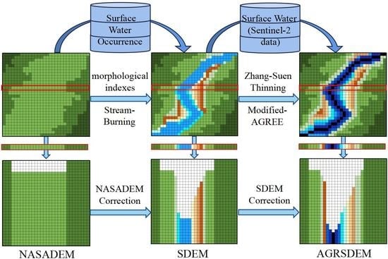
2.1. Processing of SWO and DEM Correction Based on the Stream Burning Approach

There are many small ponds in the Danjiangkou Reservoir area as shown in Figure 2a. These small water bodies may make the connectivity of the river network ambiguous. Therefore, SWO needs to be modified before the following DEM modification algorithm. In this paper, considering its special morphological characteristics, we classified spatially separated water bodies according to morphological index. First, the water bodies were filled with holes, and then the morphological indexes of the water bodies were calculated after the transformation of raster vectorization. The morphological indexes included the circumference, area, and the area ratio of the circumference. The preprocessing of SWO can be used to compute in the following Formula (1).
p e r i m e t e r a a r e a b p e r i m e t e r / a r e a c = n o n w a t e r
where a r e a represents the area of the proposed water bodies based on SWO, and p e r i m e t e r represents the perimeter of the proposed water bodies based on SWO.
We eliminated small-scale river patches by selecting the appropriate threshold value for each morphological index. Through trial and error visually, the coefficients of a , b, and c were 1.80 (km), 0.24 (km2), and 0.0008, respectively. The result of the preprocessed SWO(PSWO) is shown in Figure 2b.
River stage information based on SWO can be used to identify the difference of vertical limit in the inter-tidal zone to supplement the topographic information of the actual flow channel. We added PSWO as a burnt layer to DEM to force flow direction and improve the modeling of DEM surface restoration between alluvial floodplains within morphological units. Then, the high-resolution temporal information of PSWO was integrated and inherited by the stream-burning method to generate conditional DEM. To simplify the stream-burning model, the elevation of the DEM was lowered using a PSWO water mask. The PSWO value was used to establish a linear function of elevation relative difference to guide the inward flood simulation towards the enhancing water flow reinforcement, the expression is given as follows:
S D E M = F i l l ( D E M ) a ( P S W O )
where D E M represents the value of NASADEM, P S W O represents the value of PSWO, and a represents the burning intensity parameter.
Considering the fluctuant feature of terrain concerning the location of PSWO, we determined the burning intensity parameter using the mean slope of the PSWO. We used NASADEM to extract the slope concerning the location of PSWO and computed by the tangent value of the mean slope; the expression is given as follows:
a = m e a n ( S l o p P S W O )
where S l o p P S W O represents the value of the slope concerning the location of PSWO and a is 0.36 (tan0.34). The enhanced flow enforcement method based on NASADEM and PSWO generated SDEM. A schematic diagram for the stream-burning procedure is shown in Figure 3.

2.2. Extraction of the Skeleton Lines and DEM Correction Based on the Modified AGREE Approach

Once the Sentinel-2 image-based water data and the PSWO were ready, we obtained skeleton lines as follows. First, the sentinel-2 image and PSWO were used to form the skeleton lines layer. To better extract the water centerlines in wide channels and large lakes, we divided PSWO into seven types of images where water occurrence was greater than 95, 90, 80, 70, 55, 25, and 0 respectively. Then, we used a fast parallel thinning algorithm (Zhang-Suen Thinning Algorithm) [42] to extract the skeleton lines from seven types of images and water based on Sentinel-2 images. Among them, the small-scale river patches of water data based on Sentinel-2 images were eliminated by selecting the appropriate threshold value for each morphological index. Finally, we used the distance (Euclidean distance) to connect the nearest neighbor breakpoints of these skeleton lines through a vertex snap. To select the skeleton line of maximum PSWO values between these water images, we extracted the shortest path between the endpoints of the river network as the skeleton line of the final water body by the network analyst (Figure 4).
AGREE includes two kinds of user-specified elevation offset grids. One is the smooth modified elevation grid (SMOELEV), which integrates smoothed buffer zone into the DEM. The other is a sharp drop/raise grid (SHAGRID) for integrating the vector stream network into DEM. When the landscape pattern of the study area is complex and diverse, a reasonable smoothing buffer parameter (buffer distance) of the SMOELEV needs to be set. Therefore, we set a flexible parameter value of buffer distance based on AGREE to define flow direction, which reduces the error of river network extraction in open water where DEM lacks information concerning the actual flow path.
The buffer distance of the SMOELEV represents the surface elevation of both stream pixels and the extensive areas adjacent to stream pixels that need to be adjusted. In addition to the stream pixels, the river width obtained by SWO is closely related to the buffer distance. On these grounds, we present the modified AGREE(MAGREE) method, based on AGREE, to choose the stream centerline and PSWO to set a flexible smoothing buffer parameter value. In data processing, the buffer distance of the skeleton is juxtaposed with the smoothing buffer field of PSWO to obtain the entire final distribution region of the flexible buffer. Among them, the smoothing buffer field is determined by the PSWO distribution region whose grating value is greater than 0. MAGREE adjusts the surface elevation of SDEM to generate the AGRSDEM layer. The expression is given as follows:
A G R S D E M = S D E M b { N o r [ M a x d i s t ( b u f d i s t P S W O b u f d i s t s k e l ) ] } c ( S H A G R I D )
where S D E M represents the value of SDEM, b u f d i s t P S W O represents the euclidean buffer distance value of the skeleton line where the smoothing buffer field is determined by the PSWO distribution region, b u f d i s t s k e l represents the Euclidean buffer distance value of the skeleton line that the buffering radius is 120 (m), M a x d i s t represents the maximum value of buffer distance of b u f d i s t P S W O and b u f d i s t s k e l , S H A G R I D represents the skeleton line raster that is a two-value image (skeleton line raster is assigned as 1 and the other raster is assigned as 0), b represents correction factor of the modified elevation grid, c represents correction factor of the SHAGRID, and N o r appertain to normalization treatment of raster value within the range of flexible buffer distance. The spatial resolution of these raster image data is 30 (m). Taking the Danjiangkou Reservoir area for an example, the b is 24 and c is 52. The schematic diagram for the MAGREE procedure is shown in Figure 5.

2.3. River Network Based on AGRSDEM

The reconstructed DEM dataset can be used for river network extraction. The depression detention method (DEM preprocessing) and D8 algorithm (Surface Stream simulation) were selected to extract the river network. First, we removed the small defects of AGRSDEM by filling the sinks in the surface grid. Second, we used the D8 algorithm to determine the flow direction. The flow direction is divided by the maximum slope between the central grid and the neighboring grid. Finally, we created each pixel’s traffic accumulation layer, which is the cumulative weight of all pixels in each downhill pixel that flows into the output grid. We used a threshold value to select pixels with large flow accumulation to extract the river network. After many trial and error tests, the flow accumulation threshold was set to 20,000 pixels to separate the actual inland basin from the virtual depression.

3. Study Area and Materials

3.1. Study Area

The Danjiangkou Reservoir area, the source of the central route of the South-to-North Water Transfer Project, was chosen as the study area. It is located at the junction of the Han River and Dan River, covering an area of about 47,406.55 km2 (Figure 6). It is characterized by the north subtropical zone continental monsoon climate, abundant sunshine and rain, and four distinct seasons [43]. The spatial and temporal distribution of annual precipitation is significant, mainly concentrated from July to September [44]. The Danjiangkou Reservoir region has complex and diverse landforms, including medium-scale mountains, hills, and basins. The overall terrain is inclined from northwest to southeast, and is a complex geological structure. The reservoir has gentle topography and lower elevation than the surrounding area.

3.2. Datasets

3.2.1. NASADEM 001

The DEM dataset used in this study is the NASADEM dataset, which is generated from the Shuttle Radar Topography Mapping Mission (SRTM). It provides elevation data at 1 arc second spacing [45]. To improve geolocation accuracy, NASADEM relies on auxiliary input data sets and algorithms to fill in voids and reduce artifacts in strip elevation data. NASADEM is available free from https://0-doi-org.brum.beds.ac.uk/10.5067/MEaSUREs/NASADEM/NASADEM_HGT.001 (accessed on 23 January 2021). To solve the imaginary potholes in DEM and eliminate the oscillation of implied water surface elevation, DEM sinkholes must be filled.

3.2.2. Surface Water Occurrence

The Surface Water Occurrence (SWO) of GSW, available free from https://global-surface-water.appspot.com (accessed on 23 January 2021), provides a 30-m resolution summary of where and how often surface water occurs. It uses ortho-correction of the Landsat images spanning the past 32 years [28]. To map the spatio-temporal variability of Global Surface Water (GSW), each pixel is individually classified as water using big data exploration and information extraction, such as expert systems, visual analytics, and evidential reasoning. Classification performance, measured using over 40,000 reference points confirmed that the classifier produces less than 1% of false water detection, and misses less than 5% of water [28]. To compute SWO, the water detection (WD) and valid observations (VO) from the same months are summed. SWO > 0 was used to obtain water spatial distribution data and added to projection transformation operations to keep consistent with NASADEM.

3.2.3. Sentinel-2 Data

Developed by the European Commission and the European Space Agency (ESA), Sentinel-2A was initially launched in June 2015 to meet the operational requirements of the Copernicus programmer. Sentinel-2’s MSI data samples four spectral bands, 10 m in the visible and near-infrared (NIR) (from the United States Geological Survey(USGS) http://earthexplorer.usgs.gov (accessed on 23 January 2021)). We collected Sentinel-2 images of the Danjiangkou Reservoir area from May 2020 to August 2020. For Sentinel-2 imagery, our priority was to eliminate the cloud of the image by using the QA band. Then, we acquired high-quality images and NDWI data based on the satellite image data. We selected the maximum value of these NDWI data and extracted water based on the rule of ‘NDWI > 0′.

4. Results

Based on the analysis of the spatial distribution of the river network, we can intuitively see in Figure 7 that the river network has a very great improvement on the position of SWO and water body extracted from NDWI.

4.1. Validation and Assessment

The accuracy of river network positioning was qualitatively and quantitatively evaluated by the analogy method. To quantitatively evaluate the location extraction accuracy of the river network, we generated the minimum separation distance (offset distance) value between each river network pixel based on DEM and the nearest pixel of the reference river network. When the offset distance value is lower, the estimation of the reliability of the river network is more accurate. The reference river network was obtained by manually digitizing the centerline along the water surface on high-resolution Google and SWO images. To generate the offset distance raster image, the reference river network was converted to the binary images (the river network pixel is assigned 1 and the other raster is assigned 0).
To evaluate the accuracy of river network extraction objectively and carefully, three test areas (A, B, and C) with different hydrological characteristics and river morphologies were selected. Test area A is a typical plain river network system, with rivers and lakes interlaced and widely distributed throughout the whole area. The “B” test area possesses well-demarcated water surfaces where the relative and absolute vertical error of a DEM is less than the vertical range in floodplain morphology and flood wave amplitude. The “C” test area’s upland catchment has steep terrain, while the downstream is characterized by wide and shallow valleys with meandering rivers. In addition, we verified the river network location accuracy based on AGRSDEM by comparing it with previous products (MERIT Hydro and HydroSHEDS), which are summarized in Figure 8.
Considering that the resolution of the Sentinel data introduced was 10 m, we converted the river network into raster data with a resolution of 10 m. Then, we calculated the minimum separation distance (offset distance) between each pixel of the river network based on these DEM data (NASADEM 001, AGRSDEM, HydroSHEDS, MERIT Hydro) and the nearest pixel of the hand-painted river network. To better display the trend of the offset distance in the three test areas, we also generated the offset distance statistics in Table 1 and the histogram of the score distribution between 0 and 80, as shown in Figure 9. The statistical values included the first quartile, the second quartile and the third quartile, as well as the max, mean and the number of pixels.

4.2. Analysis of the Extracted River Network

In test area A, AGRSDEM can be used to automatically and effectively identify and extract part of the semi-natural and artificial river network compared with other data, as shown in Figure 8. However, in the region that lacks SWO and vector hydrological information or topography affected by human activities, the river network based on AGRSDEM may not fit well with those natural water bodies, even is “disconnected”. Therefore, in general, the offset distance of AGRSDEM is the smallest. For example, it has the shortest average offset distance (68.38 m), and the river network histogram moves to the direction with less offset distance than NASADEM. The river network based on AGRSDEM also contains the fewest pixels. In Table 1, the river network of AGRSDEM contains 4310 pixels, which are reduced by 15.62, 17.90 and 19.38%, respectively, compared with NASADEM V001, HydroSHEDS and MERIT Hydro.
In test area B, AGRSDEM can integrate the topographic information of hydrological data into flow direction data on the water surface, significantly correct distorted water paths, and “short-circuit” parallel streams than other data (Figure 8). Therefore, we found that the smaller the offset distance, the larger the proportion of grid to the total grid of the river network in the AGRSDEM histogram. In addition, the average offset distance based on AGRSDEM is reduced by 40.29% compared with NASADEM 001, and the pixel number is 7882, which is 10.81, 8.03 and 2.71% higher than NASADEM V001, MERIT Sheds and MERIT Hydro, respectively.
Among the three test areas, the consistency between the river network based on AGRSDEM and the reference river network is the best in test area C. It was found that in Figure 8, AGRSDEM integrates hydrological data into DEM, and the extraction of the mountain river network is closer to the actual water body. Therefore, the histogram of the river network in test area C moves to the direction with less offset distance than other test areas. It also generates the integral minimum statistics and maximum pixel count in Table 1. The calculated average value of AGRSDEM is 215.92 m, which is 42.35, 57.82 and 31.04% lower than NASADEM 001, MERIT Sheds and MERIT Hydro, respectively.
As a whole, we found some parallel streams located on or near the water shown in Figure 8. These parallel streams may represent branches that are activated during the flood period. However, these parallel streams are simpler than the actual skeleton line of river channels with a higher occurrence rate. In addition, we also found some parallel streams based on DEM located in the no-water area, and even two parallel streams located in a river channel. These parallel streams are completely different from the situation of the actual river network in our research. We used the hydrological information of SWO data, and the high-resolution skeleton line of river channels based on Sentinel-2 products, to add topographic information from the existing DEM. The river network extraction based on DEM by adding auxiliary data was closer to the actual skeleton line of river channels with a higher occurrence rate. This river network extraction may represent the actual skeleton line of river channels to the greatest extent.

5. Discussion

AGRSDEM is a DEM enhancement method that introduces multiple input data sources. The method obtained the layout and location of the river network with satisfactory results in the complex and diverse landforms. However, the extraction of an artificial river network based on AGRSDEM could not be connected. To better analyze the effectiveness of the AGRSDEM method, it is necessary to discuss the river network based on AGRSDEM from the following aspects.

5.1. Comparative Analysis of Rebuild DEM Algorithm by Using Different River Information

To test the importance of each input data, we compared the advantages and disadvantages of the river network based on reconstructed DEM with different hydrological data by intuitively judging the flow direction and river network. These DEMs mainly include the NASADEM, NASADEM based on the stream burning introducing PSWO data, NASADEM based on MAGREE introducing the vector river network, NASADEM based on AGRSDEM introducing two kinds of hydrological data (the PSWO data and the vector river network) in Figure 10.
The flow direction based on the original DEM lacks a lot of information. Most parts of the river network are incorrect and short circuits of the meandering channel. NASADEM based on the stream burning introducing PSWO data (equivalent to the RSSB based on the stream burning introducing based water depth data of MuWI), resulted in the river network being consistent with the reference river network to a certain extent. However, the flow direction data were still lacking, and some river network had errors. The NASADEM based on MAGREE introduced vector river network data, which can improve inaccurate flow paths. However, the river network was perpendicular to the river centerline, which is quite different from the natural river network. AGRSDEM combined two types of hydrological data and performed best among these reconstructed DEMs. For example, the flow direction data of the original DEM data used PSWO implicit terrain data and vector river network data to improve some obscure and irrelevant hydrological features. It also corrected the lack of detail caused by the map scale of the DEM utilized. Therefore, the river network with two kinds of hydrological data was closest to the actual river network.

5.2. Comparative Analysis of Different SHAGRID and SMOELEV Parameters of AGRSDEM

The differences between the two parameters of AGRSDEM were compared. For SHAGRID in Figure 11, the modification of flow direction is related to the value of SHAGRID. If we use a smaller SHAGRID, which fills the false sink of the reservoir basin to the level of the land surface cells, the AGRSDEM introduces less flow direction data into the original DEM. In other words, the larger the SHAGRID value is, the smaller the false sink of the reservoir basin. When the SHAGRID reaches the critical value, the reservoir area does not form the false sink. To introduce more flow direction data into the original DEM, we set the SHAGRID value to 52.
The SMOELEV in Figure 12 forms a wider “trench” in the digital landscape. The larger the SMOELEV, the less the original DEM is modified by PSWO. Even the effect of SMOELEV can completely replace the PSWO correction, and the river network based on AGRSDEM was similar to the river network based on MAGREE. However, AGRSDEM also introduces additional and unrelated river network features if the SMOELEV is too small. For application to the Danjiangkou Reservoir area, the value of SMOELEV is 24 times the normalized buffer distance value.

5.3. The Comparative Analysis of Determination of Flow Direction by Using Different Algorithms

The current main flow algorithms include Single flow Direction (SFD) and Multiple Flow Direction (MFD). SFD8 (D8) is a typical SFD algorithm selected by many researchers [46]. As for the MFD algorithm, Dinf (D-Infinity) proposed by [21] combines the advantages of the DEMON method and the Lea method to improve the SFD8 algorithm. In addition, we chose the MFD-fg (“fg” stands for “function of gradient”) algorithm [22] as the typical MFD algorithm in our study. The results showed that the river network extracted by D8, Dinf, and MFD-fg were similar. However, the river network extracted by Dinf and MFD-fg was discontinuous. The D8 algorithm had a more stable performance with the river network based on AGRSDEM compared to the other two algorithms. Therefore, the D8 algorithm was selected to extract the river network in Figure 13.

5.4. Limitations and Future Work

Despite satisfactory performance, AGRSDEM has some potential limitations that need to be noted. First, AGRSDEM needs to artificially set parameters, and is not able to perform satisfactorily in plain areas. To solve these problems in future studies, we will incorporate the hydrological data into the original flow direction to improve the river network rather than DEM. In addition, the SWO and remote sensing images used could not identify certain narrow waterways and the replacement dendritic transport path of large lakes with multiple arms/branches, leading to deviation or error in the positioning of river paths. Based on this finding, our future research will focus on enhanced flow implementation methods based on high-resolution, high-quality hydrological data.

6. Conclusions

To improve the accuracy of river network extraction in the Danjiangkou Reservoir area, a new DEM enhancement method was used. According to qualitative and quantitative evaluation methods, the validity of the proposed method was verified by comparison with the other three DEMs in three experimental basins with different topographic characteristics. The conclusions are as follows:
The hole-filling solution based on the D8 method may cause significant changes to the original terrain and produce incorrect flat areas that lack topographic information. AGRSDEM, based on the predefined flow paths by stream burning and MAGREE can provide corresponding altitude information. Thus, AGRSDEM improves the relative vertical accuracy between these units and the subsequent routing of water within the inter-tidal zone to accurately and efficiently extract the river network.
AGRSDEM has several limitations. Since it is difficult to overcome the limitations of only using water occurrence data and vector water map, our future research will consider combining the proposed method with other suitable terrain analysis methods to obtain a higher accuracy river network.

Author Contributions

Data curation, L.L., L.W. and P.Z.; Formal analysis, L.L. and L.W.; Investigation, P.Z. and F.X.; Methodology, L.L., L.W., Y.D. and F.L.; Project administration, L.W., F.L. and F.X.; Software, L.L.; Validation, L.L. and L.W.; Visualization, L.L. and F.L.; Writing—original draft, L.L., Y.D. and L.W.; Writing—review & editing, L.W., Q.Y. and F.L. All authors have read and agreed to the published version of the manuscript.

Funding

This research was funded by the National Natural Science Foundation of China (No. U22A20567 and No.51809250), the Hubei Provincial Key Research and Development Program (No. 2020BCA074), and the Science and Technology Partnership Program, Ministry of Science and Technology of China (No. KY201802007).

Data Availability Statement

Not applicable.

Acknowledgments

The authors would like to thank all the anonymous reviewers and the editor for their constructive comments and suggestions on this manuscript.

Conflicts of Interest

The authors declare no conflict of interest.

References

  1. Wang, Z.; Liu, J.; Li, J.; Meng, Y.; Pokhrel, Y.; Zhang, H. Basin-scale high-resolution extraction of drainage networks using 10-m Sentinel-2 imagery. Remote Sens. Environ. 2021, 255, 112281. [Google Scholar] [CrossRef]
  2. Wu, T.; Li, J.; Li, T.; Sivakumar, B.; Zhang, G.; Wang, G. High-efficient extraction of drainage networks from digital elevation models constrained by enhanced flow enforcement from known river maps. Geomorphology 2019, 340, 184–201. [Google Scholar] [CrossRef]
  3. Chen, X.; Long, D.; Hong, Y.; Zeng, C.; Yan, D. Improved modeling of snow and glacier melting by a progressive two-stage calibration strategy with GRACE and multisource data: How snow and glacier meltwater contributes to the runoff of the Upper Brahmaputra River basin? Water Resour. Res. 2017, 53, 2431–2466. [Google Scholar] [CrossRef]
  4. Sheng, M.; Lei, H.; Jiao, Y.; Yang, D. Evaluation of the runoff and river routing schemes in the community land model of the Yellow River Basi. J. Adv. Model. Earth Syst. 2017, 9, 2993–3018. [Google Scholar] [CrossRef]
  5. Yamazaki, D.; Ikeshima, D.; Sosa, J.; Bates, P.D.; Allen, G.H.; Pavelsky, T.M. MERIT Hydro: A high-resolution global hydrography map based on latest topography dataset. Water Resour. Res. 2019, 55, 5053–5073. [Google Scholar] [CrossRef]
  6. Shin, S.; Pokhrel, Y.; Yamazaki, D.; Huang, X.; Torbick, N.; Qi, J.; Pattanakiat, S.; Ngo-Duc, T.; Duc Nguyen, T. High resolution modeling of river-floodplain-reservoir inundation dynamics in the Mekong River Basin. Water Resour. Res. 2020, 56, 1–23. [Google Scholar] [CrossRef]
  7. Buchanan, B.P.; Archibald, J.A.; Easton, Z.M.; Shaw, S.B.; Schneider, R.L.; Todd Walter, M. A phosphorus index that combines critical source areas and transport pathways using a travel time approach. J. Hydrol. 2013, 486, 123–135. [Google Scholar] [CrossRef]
  8. Wu, Y.; Chen, J. Investigating the effects of point source and non point source pollution on the water quality of the East River (Dongjiang) in South China. Ecol. Indic. 2013, 32, 294–304. (In Chinese) [Google Scholar] [CrossRef]
  9. Garneau, C.; Sauvage, S.; Sánchez-Pérez, J.M.; Lofts, S.; Brito, D.; Neves, R.; Probst, A. Modelling trace metal transfer in large rivers under dynamic hydrology: A coupled hydrodynamic and chemical equilibrium model. Environ. Model. Softw. 2017, 89, 77–96. [Google Scholar] [CrossRef]
  10. U.S. Geological Survey. HYDRO1k Elevation Derivative Database. 2000. Available online: http://eros.usgs.gov/products/elevation/gtopo30/hydro/index.html (accessed on 28 December 2020).
  11. Lehner, B.; Verdin, K.; Jarvis, A. New Global Hydrography Derived From Spaceborne Elevation Data. Eos Trans. Am. Geophys. Union 2008, 89, 93–94. [Google Scholar] [CrossRef]
  12. Agosto, E.; Dalmasso, S.; Pasquali, P.; Terzo, O. Ithaca worldwide flood alert system: The web framework. Appl. Geomat. 2011, 3, 83–89. [Google Scholar] [CrossRef]
  13. Marthews, T.R.; Dadson, S.J.; Lehner, B.; Abele, S.; Gedney, N. High-resolution global topographic index values for use in large-scale hydrological modelling. Hydrol. Earth Syst. Sci. 2015, 19, 91–104. [Google Scholar] [CrossRef]
  14. Dirk, E.; Willem, V.V.; Dai, Y.; Albrecht, W.; Hessel, C.W.; Philip, J.W. A hydrography upscaling method for scale-invariant parametrization of distributed hydrological models. Hydrol. Earth Syst. Sci. 2021, 25, 5287–5313. [Google Scholar] [CrossRef]
  15. Wu, H.; Kimball, J.S.; Li, H.; Huang, M.; Leung, L.R.; Adler, R.F. A new global river network database for macroscale hydrologic modeling. Water Resour. Res. 2012, 48, 93–94. [Google Scholar] [CrossRef]
  16. Stanislawski, L.; Brockmeyer, T.; Shavers, E. Automated road breaching to enhance extraction of natural drainage networks from elevation models through deep learning. ISPRS-Int. Arch. Photogrammetry. Remote Sens. Spat. Inf. Sci. 2018, XLII-4, 597–601. [Google Scholar] [CrossRef]
  17. Yan, Y.; Tang, J.; Pilesjö, P. A combined algorithm for automated drainage network extraction from digital elevation models. Hydrol. Process. 2018, 32, 1322–1333. [Google Scholar] [CrossRef]
  18. Du, C.; Ye, A.; Gan, Y.; You, J.; Duan, Q.; Ma, F.; Hou, J. Drainage network extraction from a high-resolution DEM using parallel programming in the NET Framework. J. Hydrol. 2017, 555, 506–517. [Google Scholar] [CrossRef]
  19. Bai, R.; Li, T.; Huang, Y.; Li, J.; Wang, G.; Yin, D. A hierarchical pyramid method for managing large-scale high-resolution drainage networks extracted from DEM. Comput. Geosci. 2015, 85, 234–247. [Google Scholar] [CrossRef]
  20. O'Callaghan, J.F.; Mark, D.M. The extraction of drainage networks from digital elevation data. Comput. Vis. Graph. Image Process. 1984, 28, 323–344. [Google Scholar] [CrossRef]
  21. Tarboton, D.G. A new method for the determination of flow directions and upslope areas in grid digital elevation models. Water Resour. Res. 1997, 33, 309–319. [Google Scholar] [CrossRef]
  22. Qin, C.; Li, B.; Zhu, A.; Yang, L.; Pei, T.; Zhou, C. Multiple flow direction algorithm with flow partition scheme based on downslope gradient. Adv. Water Sci. 2006, 17, 450–456. (In Chinese) [Google Scholar] [CrossRef]
  23. Werner, M. Shuttle Radar Topography Mission (SRTM), Mission Overview. J. Telecommun. 2001, 55, 75–79. [Google Scholar] [CrossRef]
  24. Danko, D.M. The Digital Chart of the World Project. Photogramm. Eng. Remote Sens. 1992, 58, 1125–1128. [Google Scholar] [CrossRef]
  25. Environmental Systems Research Institute. ArcWorld 1: 3 Mio: Continental Coverage; Data obtained on CD; Environmental Systems Research Institute: Redlands, CA, USA, 1992. [Google Scholar]
  26. Lehner, B.; Döll, P. Development and validation of a global database of lakes, reservoirs and wetlands. J. Hydrol. 2004, 296, 1–22. [Google Scholar] [CrossRef]
  27. Yamazaki, D.; Trigg, M.A.; Ikeshima, D. Development of a global ~90 m water body map using multi-temporal Landsat images. Remote Sens. Environ. 2015, 171, 337–351. [Google Scholar] [CrossRef]
  28. Pekel, J.F.; Cottam, A.; Gorelick, N.; Belward, A.S. High-resolution mapping of global surface water and its long-term changes. Nature 2016, 540, 418–422. [Google Scholar] [CrossRef]
  29. Haklay, M.; Singleton, A.; Parker, C. Web Mapping 2.0: The Neogeography of the GeoWeb. Geogr. Compass 2008, 2, 2011–2039. [Google Scholar] [CrossRef]
  30. Yamazaki, D.; Ikeshima, D.; Tawatari, R.; Yamaguchi, T.; O'Loughlin, F.; Neal, J.C.; Sampson, C.C.; Kanae, S.; Paul, D. A high-accuracy map of global terrain elevations. Geophys. Res. Lett. 2017, 44, 5844–5853. [Google Scholar] [CrossRef]
  31. Wang, Z.; Liu, J.; Li, J.; Zhang, D.D. Multi-Spectral Water Index (MuWI): A Native 10-m Multi-Spectral Water Index for Accurate Water Mapping on Sentinel-2. Remote Sens. 2018, 10, 1643. [Google Scholar] [CrossRef]
  32. Saunders, W. Preparation of DEMs for use in environmental modeling analysis. Esri User Conf. 1999, 24, 1–18. [Google Scholar]
  33. Hellweger, R. Center for Research in Water Resources, The University of Texas at Austin 1997. Available online: https://www.ce.utexas.edu/prof/maidment/gishydro/ferdi/research/agree/agree.html (accessed on 1 October 1997).
  34. Peng, P.; Lin, A. River System Extraction Based on AGREE Algorithm. Water Resour. Power 2015, 33, 27–29. (In Chinese) [Google Scholar]
  35. Pickens, A.H.; Hansen, M.C.; Hancher, M.S.; Stehman, V.; Tyukavina, A.; Potapov, P.; Marroquin, B.; Pickens, Z.S. Mapping and sampling to characterize global inland water dynamics from 1999 to 2018 with full Landsat time-series. Remote Sens. Environ. 2020, 243, 1–19. [Google Scholar] [CrossRef]
  36. Puttinaovarat, S.; Horkaew, P.; Khaimook, K.; Polnigongit, W. Adaptive hydrological flow field modeling based on water body extraction and surface information. J. Appl. Remote Sens. 2015, 9, 095041. [Google Scholar] [CrossRef]
  37. Li, Q.; Lan, H.; Zhao, X.; Wu, Y. River centerline extraction using the multiple direction integration algorithm for mixed and pure water pixels. GISci. Remote Sens. 2019, 56, 26. [Google Scholar] [CrossRef]
  38. Maswood, M.; Hossain, F. Advancing river modelling in ungauged basins using satellite remote sensing: The case of the Ganges–Brahmaputra–Meghna basin. Int. J. River Basin Manag. 2016, 14, 15. [Google Scholar] [CrossRef]
  39. Ujwal Deep, S.; Sohini, N.; Jhikmik, K.; Uttam, M. Lithological and tectonic response on catchment characteristics of Rishi Khola, Sikkim, India. J. Mt. Sci. 2021, 18, 3003–3024. [Google Scholar] [CrossRef]
  40. Esper Angillieri, M.Y.; Perucca, L.P. Geomorphology and morphometry of the de La Flecha river basin, San Juan, Argentina. Environ. Earth Sci. 2014, 72, 3227–3237. [Google Scholar] [CrossRef]
  41. Zhang, T.Y.; Suen, C.Y. A fast parallel algorithm for thinning digital patterns. Commun. ACM 1984, 27, 236–239. [Google Scholar] [CrossRef]
  42. Wang, L.; Huang, J.; Du, Y.; Hu, Y.; Han, P. Dynamic Assessment of Soil Erosion Risk Using Landsat TM and HJ Satellite Data in Danjiangkou Reservoir area, China. Remote Sens. 2013, 5, 3826–3848. [Google Scholar] [CrossRef]
  43. Liu, C.; Wu, X.; Wang, L. Analysis on land ecological security change and affect factors using RS and GWR in the Danjiangkou Reservoir area, China. Appl. Geogr. 2019, 105, 1–14. [Google Scholar] [CrossRef]
  44. Crippen, R.; Buckley, S.; Agram, P.; Belz, E.; Gurrola, E.; Hensley, S.; Kobrick, M.; Lavalle, M.; Martin, J.; Neumann, M.; et al. NASADEM global elevation model:methods and progress. ISPRS-Int. Arch. Photogramm. Remote Sens. Spat. Inf. Sci. 2016, XLI-B4, 125–128. [Google Scholar] [CrossRef]
  45. McFEETERS, S.K. The use of the Normalized Difference Water Index (NDWI) in the delineation of open water features. Int. J. Remote Sens. 1996, 17, 1425–1432. [Google Scholar] [CrossRef]
  46. Jenson, S.K.; Domingue, J.O. Extracting Topographic Structure from Digital Elevation Data for Geographic Information System Analysis. Photogramm. Eng. Remote Sens. 1988, 54, 1593–1600. [Google Scholar]
Figure 1. AGRSDEM framework combined stream burning, modified AGREE, and D8 algorithm to extract the river network.
Remotesensing 15 01014 g001
Figure 2. SWO map (a) and Preprocessed SWO map (b).
Remotesensing 15 01014 g002
Figure 3. Flow chart of the stream burning of originality DEM based on PSWO.
Remotesensing 15 01014 g003
Figure 4. Extraction of the skeleton lines of hydrography layers.
Remotesensing 15 01014 g004
Figure 5. The flow chart of setting a flexible parameter value of the buffering radius of modified AGREE.
Remotesensing 15 01014 g005
Figure 6. Location of the Danjiangkou Reservoir area, China.
Remotesensing 15 01014 g006
Figure 7. River network of AGRSDEM and NASADEM (the blue and red lines are the river network based on AGRSDEM and NASADEM, respectively).
Remotesensing 15 01014 g007
Figure 8. River network based on four data in three test areas.
Remotesensing 15 01014 g008
Figure 9. Histogram of river network extraction of four DEMs in the three test areas.
Remotesensing 15 01014 g009
Figure 10. Comparison maps of different reconstructed DEM (significant changes are marked in red).
Remotesensing 15 01014 g010
Figure 11. Comparison between the different sharp drop/raise grids of AGRSDEM (significant changes are marked in red).
Remotesensing 15 01014 g011
Figure 12. The comparison between the different smooth modified elevation grids of AGRSDEM (significant changes are marked in red).
Remotesensing 15 01014 g012
Figure 13. Comparison maps of different algorithms of Surface Stream Simulation (significant changes are marked in green).
Remotesensing 15 01014 g013
Table 1. The statistical value of offset distance of the river network extraction results was produced using different rebuild DEMs in the test area A, B and C.
Test AreaDataFirst
Quartile
Second
Quartile
Third
Quartile
MaxMean Number of Pixels
ANASADEM 12.8638.5779.29546.4473.735108
AGRSDEM8.6428.0979.96551.0968.384310
HydroSHEDS35.7178.13138.40569.2174.295250
MERIT Hydro19.6839.3680.90557.5872.965346
BNASADEM 19.6843.5888.56358.4761.957030
AGRSDEM9.3227.9553.24339.4136.997882
HydroSHEDS27.4556.0090.04280.0062.057249
MERIT Hydro13.9836.1064.06296.9846.357668
CNASADEM 13.7031.2260.15194.1637.458196
AGRSDEM0.0014.1430.00176.9221.598273
HydroSHEDS19.4742.3376.19215.8751.188067
MERIT Hydro9.6928.3149.92190.0031.318005
Disclaimer/Publisher’s Note: The statements, opinions and data contained in all publications are solely those of the individual author(s) and contributor(s) and not of MDPI and/or the editor(s). MDPI and/or the editor(s) disclaim responsibility for any injury to people or property resulting from any ideas, methods, instructions or products referred to in the content.

