Technical Note

Study on Rapid Inversion of Soil Water Content from Ground-Penetrating Radar Data Based on Deep Learning

1
College of Geo-Exploration Science and Technology, Jilin University, 938 Ximinzhu Street, Changchun 130026, China
2
Shaanxi Land Engineering Construction Group Co., Ltd., Xi’an 710075, China
*
Author to whom correspondence should be addressed.
Submission received: 27 February 2023 / Revised: 24 March 2023 / Accepted: 30 March 2023 / Published: 2 April 2023
(This article belongs to the Special Issue Remote Sensing of Soil Moisture for Agricultural Purposes)

Abstract

:
Ground-penetrating radar (GPR) is an efficient and nondestructive geophysical method with great potential for detecting soil water content at the farmland scale. However, a key challenge in soil detection is obtaining soil water content rapidly and in real-time. In recent years, deep learning methods have become more widespread in the earth sciences, making it possible to use them for soil water content inversion from GPR data. In this paper, we propose a neural network framework GPRSW based on deep learning of GPR data. GPRSW is an end-to-end network that directly inverts volumetric soil water content (VSWC) through single-channel GPR data. Synthetic experiments show that GPRSW accurately identifies different VSWC boundaries in the model in time depth. The predicted VSWC and model fit well within 40 ns, with a maximum error after 40 ns of less than 0.10 cm3 × cm−3. To validate our method, we conducted GPR measurements at the experimental field of the Academy of Agricultural Sciences in Gongzhuling City, Jilin Province and applied GPRSW to VSWC measurements. The results show that predicted values of GPRSW match with field soil samples and are consistent with the overall trend of the TDR soil probe samples, with a maximum difference not exceeding 0.03 cm3 × cm−3. Therefore, our study shows that GPRSW has the potential to be applied to obtain soil water content from GPR data on farmland.

1. Introduction

At present, there are 1.5 billion square hectares of cultivated land area all over the world. Soil moisture, as a significant factor in agricultural development, has a direct impact on crop yield. For example, in the case of rice, the yield of rice at maturity changes accordingly as the soil moisture content gradually changes within a rice field [1]. Similarly, there will be a significant difference in corn yield under different soil moisture contents in the field [2]. With the promotion of precise agriculture, it is of great practical significance to measure the soil water content rapidly and accurately in the field, which will guide the area and amount of irrigation water and achieve maximum agricultural benefits.
At this stage, there are many methods available for detecting soil water content. According to the detection range, soil water content detection can be classified into three scales: small, medium, and large scale. Small-scale detection methods include the drying method [3], time-domain reflectometry (TDR) method [4], and neutron probe method [5]. Small-scale detection results are accurate but easily affected by terrain, landscape type, and soil heterogeneity. Therefore, it is difficult to represent soil moisture information on a regional scale and impossible to quickly evaluate the overall water content distribution range in farmland [6]. Medium-scale methods mainly include GPR technology, such as the radar signal attribute method (RSAM) [7], borehole radar method [8], common-offset GPR method, and multi-offset GPR method [9,10,11]. These methods have a high resolution, strong anti-interference ability, so that a system or device is capable of resisting or rejecting external interference signals that may affect its performance or accuracy; integrated data acquisition and processing imaging, nondestructive for soil structure; and perform well in farmland water content detection, but the data inversion process is relatively complex. Large-scale methods mainly include remote sensing, such as the thermal infrared method [12], proximal visible–near infrared spectroscopy method [13], and microwave remote sensing method [14,15]. These methods can quickly obtain the distribution of soil moisture content on the surface of the land over a large range but are limited at very shallow detection depths. In addition, the detection accuracy of these methods is easily affected by weather conditions. Therefore, these methods are not suitable for detecting soil moisture content at the farmland scale.
In previous research, a multi-offset GPR method has been primarily used to measure soil water content on agricultural plots, specifically the ground wave method and reflected wave method. The ground wave method can obtain the average soil water content on the upper measurement line but cannot provide quantitative measurements of soil water content at each point on the measurement line [16]. The reflected wave method is able to obtain soil water content and soil depth when the soil has a clear reflected layer but is not applicable when the soil is not clearly stratified. However, a multi-offset GPR method requires multiple movements of the receiving antenna to collect data, which requires a significant amount of time and work.
In recent years, deep learning technology has rapidly developed in various fields, such as image processing [17], medical image reconstructions [18], electrical resistivity inversions [19,20], and seismic inversions [21]. Deep learning has proven to possess exceptional power and accuracy in extracting the internal relationship between data variables in data sets. In the field of earth science, deep learning has seen significant applications. Zheng et al. [22] utilized a convolutional neural network (CNN) to automatically identify defects in 3D seismic data volumes and predict one-dimensional velocity models and underground density profiles. Araya-Polo et al. [23] extracted similarities from raw seismic data to predict velocity models. Wu and Lin [24], Yang and Ma [25], and Li et al. [26] applied CNN-based architectures to directly predict two-dimensional (2D) velocity models from original seismic waveforms to support multi-offset, multi-wave seismic acquisition for oil and gas exploration. Deep learning is also utilized in GPR signal recognition, target object detection, and GPR data inversion. In the field of GPR signal recognition, Pham et al. [27] used a pretrained Faster R-CNN framework for GPR image recognition, and the detection results confirmed that deep learning methods outperformed traditional machine learning methods in terms of accuracy. Based on this, Lei et al. [28] developed a double-cluster search estimation and column-based transverse filter point algorithm in order to recognize hyperbolas in GPR images. Hyperbola fitting in the hyperbola region detected by the Faster R-CNN can automatically and efficiently extract hyperbola features but cannot decode other features. Li et al. [29] proposed a method for identifying parabolic targets of different sizes and cavities in subsurface soil or concrete structures based on YOLO v3. Experimental results showed that the V-IoU method combined with non-maximum suppression (NMS) can accurately extract targets in GPR images and reduce false recognition frames. In the field of target object detection, S. Khudoyarov et al. [30] proposed a framework for applying 3D convolutional neural networks to 3D GPR data and classifying unclassified 3D GPR data collected from urban roads in Seoul, Korea. Validation results showed that four subsurface objects (pipes, voids, manholes, and subsoil) were successfully classified with an average classification accuracy of 97%. Gao et al. [31] used a deep learning-based intelligent detection method for subsurface targets to achieve high-accuracy detection of subsurface targets on urban roads through feature extraction and classification recognition of subsurface targets. Yang et al. [32] applied a fast R-CNN target detection algorithm in deep learning to GPR image recognition and constructed a target detection model for soil and rock dam disease identification with an average accuracy of over 90%. In the field of GPR data inversion, Tong et al. [33] used CNN to achieve 3D reconstruction of the cleft. Alvarez et al. [34] proposed a deep learning framework for converting GPR maps into subsurface permittivity maps. Leong et al. [35] proposed and developed a data driven-based GPR velocity inversion technique by employing deep learning. Giannakis et al. [36] proposed a DNN-based orthorectification method and then added the proposed fast forward method to the FWI network to improve the inversion efficiency.
In order to obtain soil water content on the farmland scale in a fast and real-time method, we explored the feasibility and potential of deep learning techniques in predicting soil water content from common-offset GPR data. In this paper, we utilized the open-source software GPRNet proposed by Leong et al. [37] to develop a GPRSW neural network framework. Specifically, we used CNN neural networks to map relationships between GPR data and VSWC and proposed a GPRSW neural network framework. First, we introduced the basic theoretical concept of using deep learning to invert soil water content and explained the GPRSW neural network model and its structure in detail. After that, we generated the training datasets about GPR data and VSWC, trained the GPRSW neural network, and predicted synthetic samples through synthetic simulations. The entire training process and evaluation metrics are presented in this paper. Finally, we carried out the field experiment at the Gongzhuling Academy of Agricultural Sciences, Changchun City, Jilin Province to examine the practical application of GPRSW. The comparison of water content inverted by GPRSW, the TDR detection data, and the soil sampling value shows that the water content inversion of GPRSW can be completed in nearly ten seconds with relatively stable accuracy and a maximum error of less than 0.03 cm3 × cm−3.

2. Materials and Methods

2.1. Principle of VSWC Inversion Based on Deep Learning

GPR transmits high-frequency electromagnetic waves into the subsurface using the transmitting antenna. These waves are reflected and scattered when they encounter target bodies with different dielectric properties. Parts of the waves are filtered by the subsurface medium, transmitted back to the surface, and received by the receiving antenna [38]. The received signal is processed and converted into a time-series signal. The time series at each measurement point is the radar waveform recording channel of the measurement point. The characteristics of the radar waveform can be analyzed to determine the stratigraphic structure, the distribution of different materials underground, and the size and depth of the target body with different dielectric properties.
The characteristics of radar waveforms returned by high-frequency electromagnetic waves propagating in materials with different dielectric properties are distinct. The permittivity of unsaturated soil is mainly determined by the VSWC. As the volumetric water content in soil changes, electrical conductivity and permittivity will vary greatly. To establish the relationship between the soil permittivity and VSWC, many theoretical and empirical models have been proposed by researchers. Among them, the TOPP formula is the most widely used [39]:
θ = 5.3 × 10 2 + 2.92 × 10 2 ε r 5.5 × 10 4 ε r 2 + 4.3 × 10 6 ε r 3
where θ is the VSWC and ε r is the relative permittivity. This formula is especially suitable for coarse soil (cultivated soil).
The characteristics of radar waveform traces are closely related to the soil permittivity, which is in turn related to the VSWC. Therefore, the characteristics of radar waveform traces are closely related to the VSWC. In our study, the relationship between the radar waveform traces, S, and the VSWC, θ, can be appropriately described as:
θ = F 1 S
where F−1 is the inverse operator which calculates the desired θ from the given S. In traditional physics-based full-waveform inversion, S is the time-domain data of common-offset GPR, and F−1 is the full-waveform inversion operator, which represents the calculation of deep learning neural network in our data-driven inversion.

2.2. The Structure of CNN-Based Framework GPRSW

The CNN-based framework GPRSW is essentially an encoder–decoder model which maps the GPR data and its corresponding VSWC in a nonlinear way. Its structure is illustrated in Figure 1.
In the GPR data-encoding stage, the feature encoder network is used for down-sampling and feature extraction, which in turn generates abstract high-level features. These features are a high-level semantic description of the GPR data learned by multiple layers of neural networks, and they provide adequate information for the output of VSWC curves. At first, the time-domain GPR A-scan data is compressed using a Conv layer and Pool layer, which reduces the dimensionality of the GPR data, reserves important information, and extracts the abstract high-level features of A-scan. The extracted features are merged in the Diconv layer after four down-sampling processes and four layers of Diconv layers with different convolutional expansion rates. Finally, Mgconv is used as the bottleneck layer of the encoder. To ensure the scale diversity of the features, both the bottleneck layer and the Pool4 layer are connected to the decoder.
In the VSWC decoding stage, the features of the GPR data formed by the encoder are mainly up-sampled, and finally, the VSWC inversion result consistent with the length of the GPR data sequence is formed. The potential nonlinear relationship between the GPR data and VSWC is stored in the whole network and its parameter matrix. Convolutional layer + up-sampling is used to decode the features formed by the GPR data, recover the sequence length structure after four up-sampling and invert the GPR features into VSWC curves, and finally, output VSWC curves with the same length as the GPR data sequence by a 1 × 1 Conv convolutional layer. To avoid the instability of the network output and improve the generalization of the structure, a Gaussian dropout operation is adopted before the final output of the network.
This network is essentially an end-to-end inversion program, where an A-scan from 0 to 100 ns is applied to its input and a curve of volumetric water content at the same position with the same size is applied to its output. However, we recognize that the accuracy of the volumetric water content obtained from the inversion decreases as the depth of the time series increases. This is caused by a decrease in the quality of the A-scan due to factors such as multiple reflections. The inverse correspondence between A-scan and single-channel VSWC is shown in Figure 2.
Table 1 shows the output shapes and other configurations of all layers. In the structure of the network, ReLu is used as the activation layer, the Padding is set to “same”, and Adam’s algorithm is used as the optimization method [40,41].

2.3. Data Preparation and Network Training

To enhance the ability of the neural network to capture the relationship between the GPR data and VSWC, 10,000 pairs of data were generated into a dataset. The dataset comprises time-domain GPR data and random VSWC corresponding to it. The VSWC ranges from 0 to 0.5 cm3 × cm−3, which covers most of the soil water content fugacity. The dataset was generated by performing the following steps: (1) 10,000 pairs of relative permittivity were generated, all with a longitudinal depth of 1280 grid numbers. Of these, 7000 sets were randomly generated 1D data and 3000 sets were 1D data obtained by randomly selecting 5 traces from each of the 600 randomly generated 2D profiles, with randomly generated relative permittivity values ranging from 1 to 40, randomly generated layer numbers ranging from 4 to 12, and randomly generated layer thicknesses ranging from 8 to 15. (2) Forward simulation using the 2D finite difference time domain (FDTD) [42] was used to obtain the GPR data series corresponding to the relative permittivity. We used a standard black Harris wavelet as the source wavelet, with a center frequency of 120 Mhz, a sampling interval dt of 8 × 10⁻¹¹, and a time window t of (1280 − 1) × dt. (3) The TOOP formula was used to convert the relative permittivity to the corresponding VSWC ranging from 0 to 0.5 cm3 × cm−3.
The generated data pairs were divided into 90% training data and 10% validation data. The coefficient of determination (R Squared, R2) was used as the evaluation function to evaluate the performance of the current training model. The evaluation metric mainly evaluates the performance of the model during the training process. The R2 is expressed as follows:
R 2 = 1 i = 1 n   y ^ i y i 2 i = 1 n   y ¯ i y i 2
where y i ˙ represents the true value, y ^ i represents the predicted value, and y ¯ i represents the average value of the true value. The value of R2 ranges from 0 to 1. When R2 = 0, it means that the neural network model is completely unable to predict the target variable and that the VSWC value predicted by GPRSW from the time-domain GPR data series is completely inconsistent and unrelated to the true value. If R2 = 1, it means the neural network model is able to predict the target variable perfectly and the VSWC value predicted by GPRSW from the time-domain GPR data is completely consistent with the VSWC value in the true model.
The root-mean-square (RMS) error loss function is used as a loss function, which calculates the difference between the predicted value Y ^ and the true value 𝑌. The mean-square error loss function is often used in regression problems, and its expression is as follows:
l o s s Y , Y ^ = 1 N Σ i = 1 N y i ˙ y ^ i 2
where y i ˙ represents the true value and y ^ i represents the predicted value. The value of l o s s Y , Y ^ is non-negative, and the closer the value of l o s s Y , Y ^ is to 0, the smaller the difference between the VSWC value predicted by GPRSW from the time-domain GPR data and the VSWC value in the real model, and the better the prediction effect.
Prior to formal training, we processed the GPR data sequence to eliminate the direct wave. The training process (Intel(R) Core(TM)i5-10500 CPU @310GHz 3.10GHz) takes ~2 h. Figure 3 shows the variation in the R2 score and loss with the number of training epochs for the training and validation data after training. The neural network was set to automatically stop training when upon reaching 160 epochs. Finally, the evaluation index 𝑅2 for the training set was approximately 0.991524, and the RMS was approximately 0.000001. The evaluation of the validation set yielded an R2 value of approximately 0.9748 and RMS loss of approximately 0.00005, which indicates that the neural network model is well-trained. The predicted VSWC values obtained by GPRSW from the time-domain GPR data are closely aligned with the real model with a high degree of fit.

2.4. Principle of Field Soil Sampling and TDR Soil Probe Samples

2.4.1. Principle of Field Soil Sampling

We use the drying method to measure the soil moisture content of field soil samples. The principle of this method is based on the fact that the water content of a soil sample can be determined by measuring the difference in weight before and after drying the sample. To collect field soil samples, a soil corer or auger is used to collect soil samples from different depths in a specific area. The samples are then weighed, and the moisture content is determined by drying them in an oven until they reach a constant weight. The difference in weight before and after drying is used to calculate the moisture content of the soil sample.
One advantage of using field soil samples is that they provide highly accurate measurements of soil moisture content. However, this method is time-consuming, and it can be challenging to collect representative samples that accurately reflect the soil moisture content of a larger area.

2.4.2. Principle of TDR Soil Probe Samples

We used TRIME-PICO TDR for fixed point sampling. TDR soil probes are a commonly used method for measuring soil moisture content. The principle behind the method is based on the fact that the permittivity of soil changes with water content. TDR soil probes send a low-energy electromagnetic pulse through the soil and measure the time it takes for the pulse to reflect back to the probe. The time delay is directly related to the permittivity of the soil, which can be used to calculate the soil moisture content.
One advantage of using TDR soil probes is that they provide real-time measurements of soil moisture content, which can be useful for irrigation scheduling and other applications that require immediate data. Additionally, TDR soil probes can be used to measure the soil moisture content at different depths, which can provide a more comprehensive picture of the moisture content of a specific area of soil. Similar to the field soil samples method, one limitation of using TDR soil probes is that they also may not be able to collect representative samples that accurately reflect the soil moisture content of a larger area.

3. Results

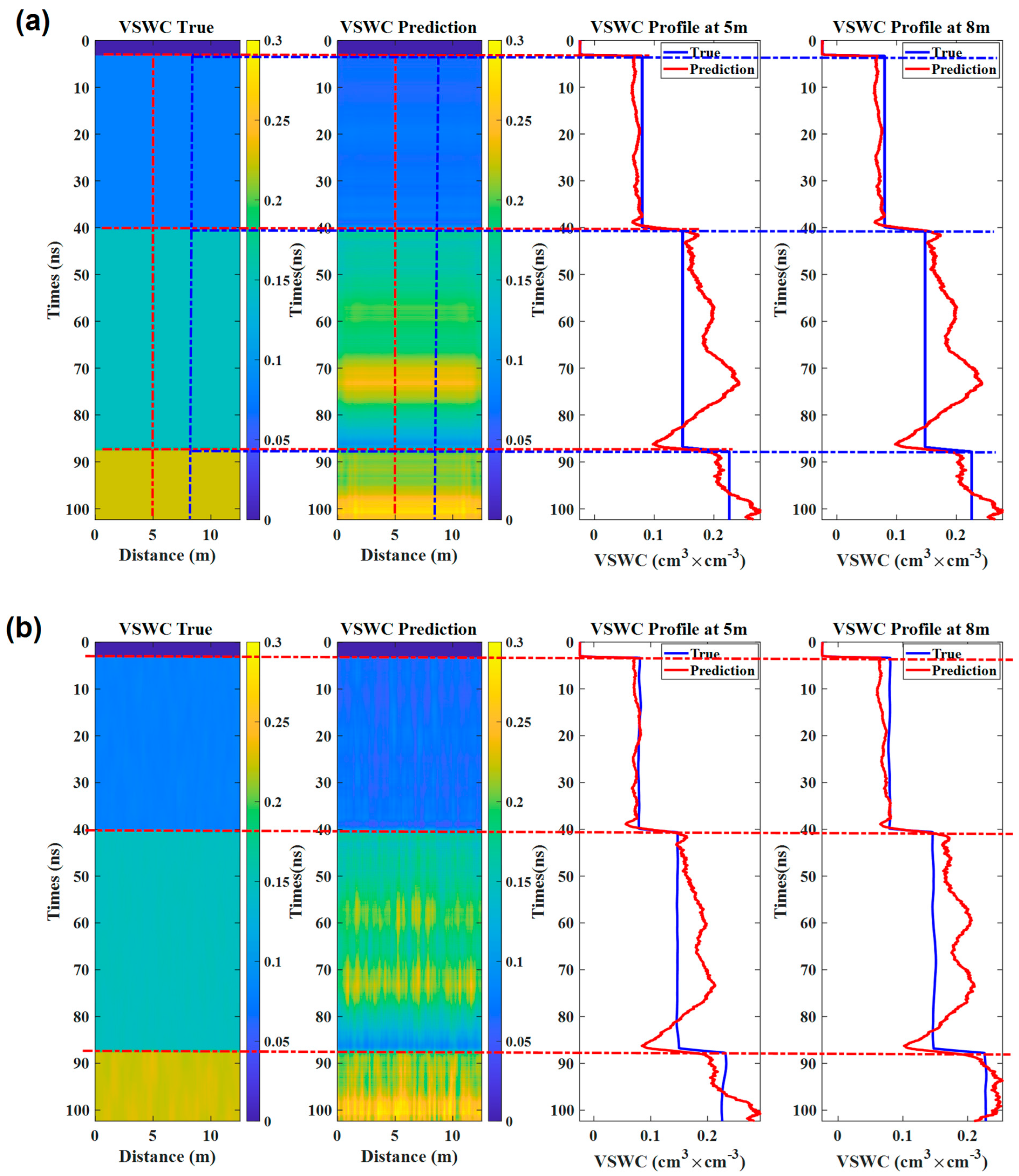
3.1. Synthetic Experiments

Two-dimensional models were established to validate the predictive effect of GPRSW on B-scans, which refer to the collection of all A-scans. Single-channel data were extracted from each model to validate the predictive effect of A-scans. Four 2D models of VSWC were established for different media types, including horizontal layered media, horizontal stochastic media, undulating-interface layered media, and undulating-interface stochastic media. These models were then converted into corresponding relative permittivity models using the TOOP formula, and the FDTD was utilized for forward simulation to obtain the GPR data series. The relative permittivity distribution and time-domain GPR data for the model are shown in Figure 4. To evaluate the effectiveness of the GPRSW neural network model, GPRSW was employed to predict the volumetric water content values from the time-domain GPR data, and two predictions (A-scans) at 5 m and 8 m were compared to the true model data; it took less than 10 s to predict.
In Figure 5a, the red dotted line accurately separates the four media, and the predicted values fit the true values well from 0 to 40 ns. In Figure 3b, the degree of fit between the predicted value and the model value is very high within 0–40 ns, and the maximum error between the predicted VSWC and the true value is less than 0.10 cm3 × cm−3, which is slightly better than that in Figure 3a. In Figure 3c, the boundary of VSWC is accurately separated at 5 m and 8 m, and the maximum error between the overall predicted VSWC value and the true value is less than 0.10 cm3 × cm−3. However, the overall prediction is slightly worse than the horizontal medium prediction. In Figure 3d, the boundary of VSWC at 5 m and 8 m is accurately separated, and the overall prediction is slightly better than that in Figure 3c but slightly worse than the horizontal medium prediction. The results of the synthetic experiments showed that GPRSW can accurately predict the VSWC values at different locations in the model.

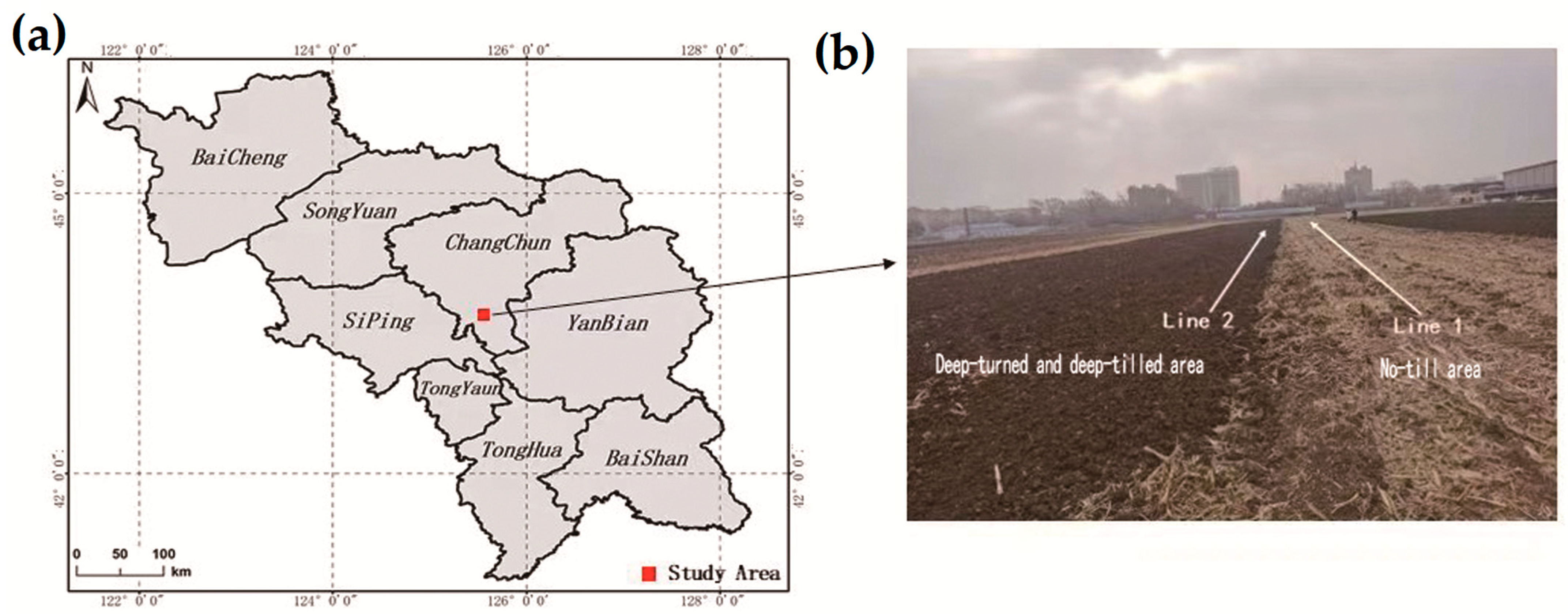
3.2. Field Experiments

In this section, the performance of GPRSW was tested using field GPR data detected by Mala ProEx radar with the radar parameters shown in Table 2. We took field soil samples and TDR soil probe samples for comparative experiments. The different working methods are shown in Figure 6. The experimental site was located in the experimental field of Gongzhuling Academy of Agricultural Sciences, Changchun City, Jilin Province. The experimental site included two experimental fields with different farming methods. The soil there is black soil, and the crops are corn all year round. Black soil is a type of soil that is known as the “golden land” for agriculture and is widely distributed in northeastern China, including Heilongjiang, Jilin, and Liaoning provinces. It is suitable for growing crops such as soybeans, corn, and sorghum. This soil is rich in organic matter and has a high clay content, making it very fertile and able to retain water well. Even in areas with dry and low rainfall, black soil can support crop growth.
Since 2011, the two experimental fields have been cultivated in different ways: one uses a no-till method which directly mulches straw without tillage at all, and the other uses a deep-turn and deep-till method, in which all corn stalks are broken up and returned to the field after deep turning and deep tilling, with a depth of 30–40 cm. The no-till area has a dense soil surface structure, while the deep-turned and deep-tilled area has a looser soil texture. During the experiment, there were no crops planted in the farmland, and the land was relatively flat. Therefore, it was suitable for GPR to detect soil water content.

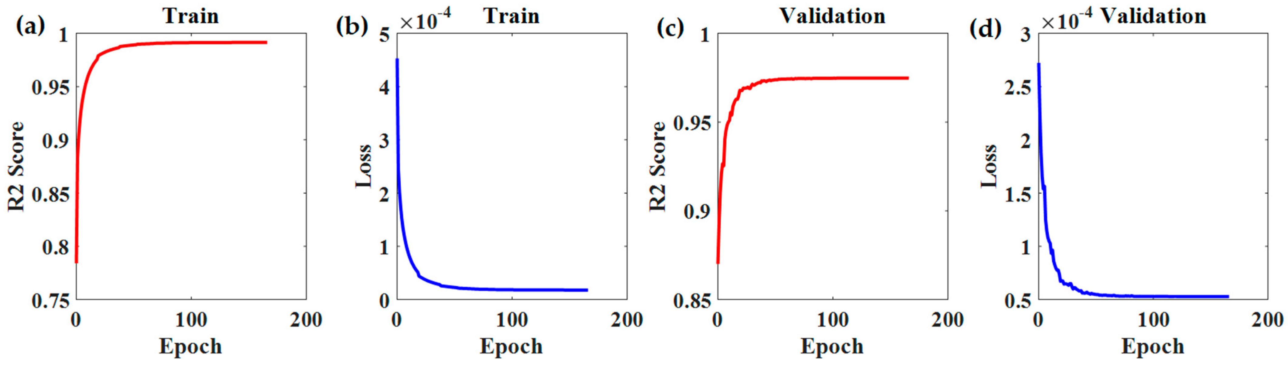
3.2.1. Data Preparation and Network Training

To encapsulate a larger range of VSWC variations, we randomly generated multilayer permittivity datasets ranging from one to fifty and converted them into VSWC profiles using the TOOP formula. An amount of 50,000 unique VSWC profiles were generated, corresponding GPR data, and were simulated using the FDTD method. For the measured field data, which usually contain high levels of noise, and common-offset GPR data, we added random Gaussian noise to expand the data set. In addition, we simulated the variation in the true subsurface horizontal velocity by adding a stochastic time gain. At the same time, we added some GPR data with corresponding relationships and field VSWC measured by TDR for fine-tuning the optimization of the network. Finally, we generated 100,000 datasets, of which 1% were used for validation, with a smooth training process and a final validation R2 accuracy of 0.9658.

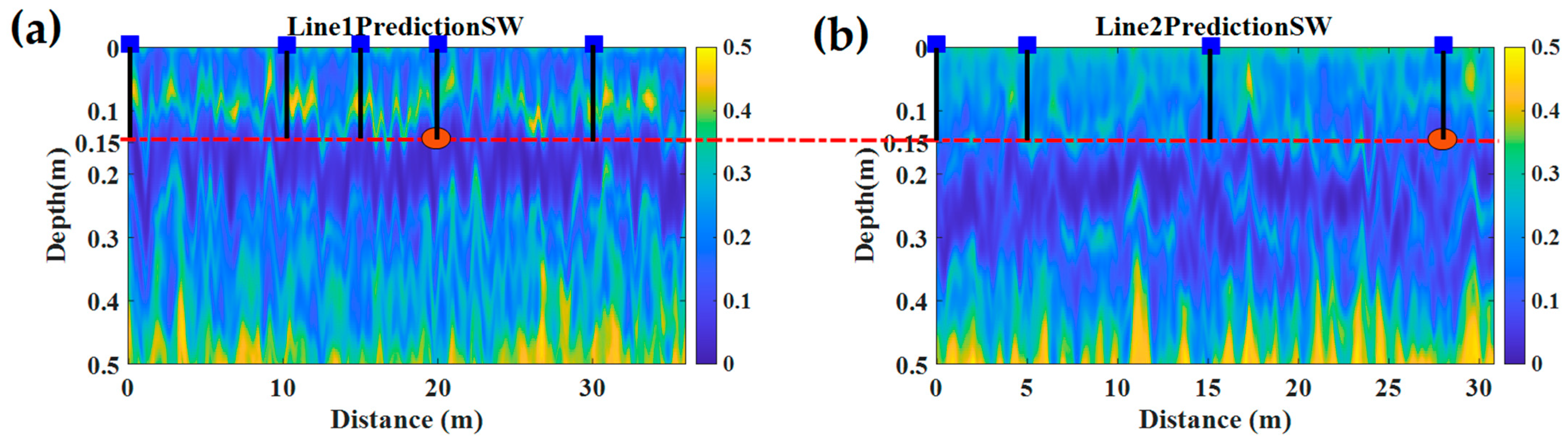
3.2.2. Inversion of Volumetric Soil Water Content in Farmland Fields

The measurement of survey line 1 with a length of 35 m was carried out in the no-till area. The measurement of survey line 2 with a length of 30 m was carried out in the deep-till and deep-turn region, as shown in Figure 7a,b. The GPR measurements had a total of 721 and 627 traces collected, respectively. This process took approximately 15 min.
B-scan collected under line 1 and line 2 was pre-processed using direct wave removal, band-pass filtering, and time gain. After that, the water content of the field data was inverted by GPRSW. It took less than 10 s to predict. The field GPR data and inversion results are shown in Figure 8 and Figure 9.

3.2.3. Field Soil Samples and TDR Soil Probe Samples

Random soil sampling was conducted next to two survey lines at a depth of approximately 15 cm, and spot probe soil sampling was also conducted using TDR at a depth of approximately 15 cm. Soil sampling was conducted at 20 m next to survey line 1 and at 27 m next to survey line 2. The TDR was spotted at positions 0 m, 10 m, 15 m, 20 m, and 30 m on survey line 1, and at positions 0 m, 5 m, 15 m, and 27 m on survey line 2. During the soil sampling process, each excavation, soil extraction, and backfill took approximately 5 min. The process for two locations took about 10 min. The TDR probe spotting process took about 30 s per spot, with a total of nine spots taking approximately 5 min. Table 3 and Table 4 show the detailed information of field soil samples and TDR probe samples, respectively.

3.2.4. Comparison Verification

In order to further validate our prediction model, we transformed the VSWC distribution information from the time domain to the spatial domain based on:
d = v t 2
where v is the EM velocity, ε r can be obtained from VSWC via Topp’s formula, v can be obtained by converting v = c ε r , d is the thickness of each layer, and t is the one-way travel time of the EM wave to the boundary between layers.
The time-domain VSWC was transformed into the spatial domain according to the dual-traveling characteristics of the common-offset GPR data in Figure 10. The locations of the measurement points in the previous section were marked in Figure 10a,b to facilitate comparison with the actual measured values. It can be clearly seen from the inversion results of spatial domain that there is an undulating interface within 0.1~0.3 m below survey line 1 and an undulating interface within 0.15~0.35 m below survey line 2. The thickness of the soil cultivation layer is about 30~40 cm, and it is inferred that the undulating layer is the bottom layer of the cultivation layer. Above 15 cm depth, the soil water content under survey line 1 is obviously higher than that under survey line 2. We infer that it is because the straw on the surface of the land in the no-till area intercepts and preserves a lot of water vapor from the air.
Table 5 shows the details of the VSWC values obtained by different methods at 15 cm depth. Additionally, a scatter plot was created for a more visual comparison and validation. As shown in Figure 11, the VSWC at the depth of 15 cm under the two survey lines predicted by GPRSW were compared with the field sampling value and TDR probe sampling value. It was found that the predicted VSWC value under line 1 was consistent with the TDR probe sampling value but slightly higher than the TDR probe sampling value. At 20 m, both were slightly lower than the field soil sampling VSWC value, and the predicted value was closer to it. For line 2, the predicted VSWC value was consistent with the trend of the TDR probe sampling values and slightly higher than the TDR probe sampling value. At 27 m, the predicted value was slightly higher than the field soil sampling value, while the TDR probe sampling value was consistent with it. In summary, the difference between the soil water content at 15 cm depth under the two lines predicted by GPRSW and the field sampling and TDR probe sampling was less than 0.03 cm3 × cm−3, which shows high prediction accuracy and good results in the field experiment.

4. Discussion

As the most direct way to detect soil water content, field sampling has the highest accuracy for the detection of physical properties at the measurement point. However, field sampling is destructive, and the difficulty of detection increases when the detection depth increases. In addition, soil samples are time-consuming and laborious to collect and still require post-processing in the laboratory to obtain the VSWC values. As a soil layer sampling method, it is not suitable for the detection of soil volume water content at the farmland scale.
As a very mature water content detection method, TDR spot sampling has high accuracy and has been widely used in field spot measurements. However, its detection range is small, and the detection depth is limited, which is still not suitable for farmland-scale VSWC detection.
The common-offset GPR method is compact, lightweight, portable, easy to operate, fast, and suitable for farmland-scale detection and research. In this paper, the deep learning method was used to inverse VSWC from the measured time-domain GPR data. The synthetic experiments and field experiments show that it can be used as an effective method for the rapid detection of VSWC in the field. In the practice of guiding agriculture to obtain farmland water content in the future, the application of real-time VSWC inversion can be realized on the premise of completing training, which has great development potential.
The mean value of VSWC measured by TDR in the no-till area was 28.44%, with the field soil sample value at 28.4%. On the other hand, the mean value of VSWC measured by TDR in the deep-turned and deep-tilled area was 20.65%, with the field soil sample value at 20.86%. The VSWC in the no-till area was generally higher than that in the deep-turned and deep-tilled area at the same detection depth. The predicted values of GPRSW on both survey lines were consistent with these findings. We analyzed the reason why the VSWC in the deep-turned and deep-tilled area was low at this depth: The soil in this area is soft after artificial ploughing, and the protective effect of the soil surface layer on water is weakened, which makes part of the water in the soil loose in the air. At the same time, ploughing makes the porosity of the soil layer smaller and the water-bearing space smaller. Most of the GPR values of soil water are higher than TDR values. We believe that one possible explanation for this difference is that the two methods measure different volumes of soil. GPR detects a larger area, which may be more sensitive to water in larger pores and cracks within the soil, while TDR may be more sensitive to water in smaller pores closer to the TDR probe. Additionally, other factors, such as soil texture and structure, may affect GPR measurements and lead to differences between GPR and TDR values.
Our study is highly relevant to precision agriculture, which requires accurate and efficient measurement of soil moisture content to optimize irrigation and fertilizer use for efficient agricultural production. GPR based on deep learning technology has advantages for quickly and accurately estimating soil moisture content, which can help farmers achieve precise irrigation and fertilizer application, resulting in improved crop yield and quality. Although our method has shown promising results, there are potential challenges and limitations when applying it to different soil types and environmental conditions. For instance, we can only estimate the volumetric water content of the soil, and further research is necessary to explore the impact of soil mineral content on GPR-based soil moisture measurements. Additionally, the accuracy of GPR may be affected by soil type and moisture distribution, which require adjusting parameters and optimizing algorithms for different soil types. Moreover, environmental factors such as weather and terrain may also impact the applicability and reliability of GPR technology, necessitating more field experiments for validation. Therefore, it is crucial to comprehensively consider and systematically optimize and adjust the technology to ensure its effectiveness and practicality in real-world applications. In future research, we will use more GPR data and corresponding farmland VSWC data to further improve the neural network model so that GPRSW can be applied to many different types of cultivated land VSWC measurements, which will help farmers to scientifically deploy farmland water content to increase crop yields.

5. Conclusions

In this paper, a neural network framework GPRSW for rapid inversion of VSWC by GPR was constructed to solve the difficulties of VSWC inversion using the common-offset GPR method at the field scale. After training the GPRSW model, the performance of GPRSW was tested in synthetic experiments by using four 2D VSWC models. The results show that GPRSW can accurately identify different boundaries of VSWC in the model in time depth, with a maximum error between the predicted VSWC and the true value of less than 0.10 cm3 × cm−3. Subsequently, the performance of GPRSW was tested in a Gongzhuling experimental field. The results show that there is little difference between the predicted value of GPRSW and the field soil sampling value, which is consistent with the overall change trend of the TDR detection values, with a maximum difference of less than 0.03 cm3 × cm−3. The overall study shows that GPRSW has the potential to be applied to the soil water content inversion by using GPR data on farmland.

Author Contributions

Conceptualization, Z.L., Z.Z., Q.L., R.L. and L.X.; methodology, Z.L. and H.X.; validation, Z.Z., H.X., Q.L., J.Y. and Q.L.; writing—original draft preparation, Z.L. and H.X.; writing—review and editing, Z.Z., H.X., B.A., Q.L., J.Y., H.W. and K.L. All authors have read and agreed to the published version of the manuscript.

Funding

This research was funded by the Technology Innovation Center for Land Engineering and Human Settlements, Shaanxi Land Engineering Construction Group Co., Ltd. and Xi’an Jiaotong University (grant number: 2021WHZ0080) and the 2022 Science and Technology Benefiting the People Project of Ningxia Hui Autonomous Region (grant number: 2022CMG03006).

Data Availability Statement

Not applicable.

Acknowledgments

The authors would like to thank the editors and reviewers for providing their valuable comments and suggestions. In addition, the authors also want to thank the people who participated in the GPR data measurements.

Conflicts of Interest

The authors declare no conflict of interest.

References

  1. Liu, K. Effects of Soil Moisture and Irrigation Patterns during Grain Filling on Grain Yield and Quality of Rice and Their Physiological Mechanism. Acta Agron. Sin. 2008, 34, 268–276. [Google Scholar] [CrossRef]
  2. Nielsen, D.C.; Vigil, M.F.; Benjamin, J.G. The variable response of dryland corn yield to soil water content at planting. Agric. Water Manag. 2009, 96, 330–336. [Google Scholar] [CrossRef]
  3. Li, W.; O’Kelly, B.C.; Fang, K.; Yang, M. Briefing: Water content determinations of peaty soils using the oven-drying method. Environ. Geotech. 2022, 9, 3–11. [Google Scholar] [CrossRef]
  4. Gurav, M.; Sarik, S.; Singh, K.; Pendharkar, G.; Baghini, M.S. IITB_TDR: A portable TDR system with DWT based denoising for soil moisture measurement. Sens. Actuator A Phys. 2018, 283, 317–329. [Google Scholar] [CrossRef]
  5. Evol’s’kii, S.T.; Kulik, V.V. Measurement of the moisture content and salinity of soils by steady-state neutron methods. Dopovidi Natsional’noi Akad. Nauk Ukr. 2002, 7, 146–151. [Google Scholar]
  6. Schwartz, B.F.; Schreiber, M.E.; Yan, T.T. Quantifying field-scale soil moisture using electrical resistivity imaging. J. Hydrol. 2008, 362, 234–246. [Google Scholar] [CrossRef]
  7. Zhang, W.; Bi, L.; Chang, Y.; Li, B. Estimation of soil water content of internal different layers using ground-penetrating radar signals. J. Adv. Sci. Lett. 2012, 9, 417–422. [Google Scholar] [CrossRef]
  8. Yu, Y.; Klotzsche, A.; Weihermuller, L.; Huisman, J.A.; Vanderborght, J.; Vereecken, H.; van der Kruk, J. Measuring vertical soil water content profiles by combining horizontal borehole and dispersive surface ground penetrating radar data. Near Surf. Geophys. 2020, 18, 275–294. [Google Scholar] [CrossRef] [Green Version]
  9. Weihermuller, L.; Huisman, J.A.; Lambot, S.; Herbst, M.; Vereecken, H. Mapping the spatial variation of soil water content at the field scale with different ground penetrating radar techniques. J. Hydrol. 2007, 340, 205–216. [Google Scholar] [CrossRef] [Green Version]
  10. Ardekani, M.R.M. Off- and on-ground GPR techniques for field-scale soil moisture mapping. Geoderma 2013, 200, 55–66. [Google Scholar] [CrossRef]
  11. Huisman, J.A.; Hubbard, S.S.; Redman, J.D.; Annan, A.P. Measuring Soil Water Content with Ground Penetrating Radar: A Review. Vadose Zone J. 2003, 2, 476–491. [Google Scholar] [CrossRef]
  12. Antonucci, F.; Pallottino, F.; Costa, C.; Rimatori, V.; Giorgi, S.; Papetti, P.; Menesatti, P. Development of a Rapid Soil Water Content Detection Technique Using Active Infrared Thermal Methods for In-Field Applications. Sensors 2011, 11, 10114–10128. [Google Scholar] [CrossRef] [PubMed] [Green Version]
  13. El Alem, A.; Hmaissia, A.; Chokmani, K.; Cambouris, A.N. Quantitative Study of the Effect of Water Content on Soil Texture Parameters and Organic Matter Using Proximal Visible-Near Infrared Spectroscopy. Remote Sens. 2022, 14, 3510. [Google Scholar] [CrossRef]
  14. Wagner, W.; Bloschl, G.; Pampaloni, P.; Calvet, J.C.; Bizzarri, B.; Wigneron, J.P.; Kerr, Y. Operational readiness of microwave remote sensing of soil moisture for hydrologic applications. Nord. Hydrol. 2007, 38, 1–20. [Google Scholar] [CrossRef]
  15. Wang, L.L.; Qu, J.J. Satellite remote sensing applications for surface soil moisture monitoring: A review. Front. Earth Sci. China 2009, 3, 237–247. [Google Scholar] [CrossRef]
  16. Galagedara, L.W.; Parkin, G.W.; Redman, J.D.; von Bertoldi, P.; Endres, A.L. Field studies of the GPR ground wave method for estimating soil water content during irrigation and drainage. J. Hydrol. 2005, 301, 182–197. [Google Scholar] [CrossRef]
  17. de Oliveira, L.A.; Medeiros, H.R.; Macedo, D.; Zanchettin, C.; Oliveira, A.L.I.; Ludermir, T. SegNetRes-CRF: A Deep Convolutional Encoder-Decoder Architecture for Semantic Image Segmentation. In Proceedings of the IEEE IJCNN 2018, Rio de Janeiro, Brazil, 8–13 July 2018. [Google Scholar]
  18. Han, X. MR-based synthetic CT generation using a deep convolutional neural network method. Med. Phys. 2017, 44, 1408–1419. [Google Scholar] [CrossRef] [PubMed] [Green Version]
  19. Liu, B.C.; Jiang, P.; Guo, Q.; Wang, C.W. Deep Learning Inversion of Electrical Resistivity Data by One-Sided Mapping. IEEE Signal Proc. Lett. 2022, 29, 2248–2252. [Google Scholar] [CrossRef]
  20. Liu, B.; Pang, Y.H.; Mao, D.Q.; Wang, J.; Liu, Z.Y.; Wang, N.; Liu, S.H.; Zhang, X.X. A rapid four-dimensional resistivity data inversion method using temporal segmentation. Geophys. J. Int. 2020, 221, 586–602. [Google Scholar] [CrossRef]
  21. Wu, Y.; Lin, Y.; Zhou, Z. Inversionnet: Accurate and Efficient Seismic Waveform Inversion with Convolutional Neural Networks. In Proceedings of the 2018 SEG International Exposition and Annual Meeting, Anaheim, CA, USA, 14–19 October 2018; pp. 2096–2100. [Google Scholar]
  22. Zheng, Y.; Zhang, Q.; Yusifov, A.; Shi, Y.Z. Applications of Supervised Deep Learning for Seismic Interpretation and Inversion. J. Lead. Edge 2019, 38, 526–533. [Google Scholar] [CrossRef]
  23. Araya-Polo, M.; Dahlke, T.; Frogner, C.; Zhang, C.; Poggio, T.; Hohl, D. Automated fault detection without seismic processing. J. Lead. Edge 2017, 36, 208–214. [Google Scholar] [CrossRef]
  24. Wu, Y.; Lin, Y.Z. InversionNet: An Efficient and Accurate Data-Driven Full Waveform Inversion. IEEE Trans. Comput. Imag. 2020, 6, 419–433. [Google Scholar] [CrossRef]
  25. Yang, F.S.; Ma, J.W. Deep-learning inversion: A next-generation seismic velocity model building method. Geophysics 2019, 84, R583–R599. [Google Scholar] [CrossRef] [Green Version]
  26. Li, S.C.; Liu, B.; Ren, Y.X.; Chen, Y.K.; Yang, S.L.; Wang, Y.H.; Jiang, P. Deep-Learning Inversion of Seismic Data. IEEE Trans. Geosci. Remote 2020, 58, 2135–2149. [Google Scholar] [CrossRef] [Green Version]
  27. Pham, M.T.; Lefevre, S. Buried Object Detection from B-Scan Ground Penetrating Radar Data Using Faster-Rcnn. In Proceedings of the IGARSS 2018—2018 IEEE International Geoscience and Remote Sensing Symposium, Valencia, Spain, 22–27 July 2018; pp. 6804–6807. [Google Scholar]
  28. Lei, W.T.; Hou, F.F.; Xi, J.C.; Tan, Q.Y.; Xu, M.D.; Jiang, X.Y.; Liu, G.Y.; Gu, Q.Y. Automatic hyperbola detection and fitting in GPR B-scan image. Automat. Constr. 2019, 106, 102839. [Google Scholar] [CrossRef]
  29. Li, Y.H.; Zhao, Z.X.; Luo, Y.F.; Qiu, Z. Real-Time Pattern-Recognition of GPR Images with YOLO v3 Implemented by Tensorflow. Sensors 2020, 20, 6476. [Google Scholar] [CrossRef]
  30. Khudoyarov, S.; Kim, N.; Lee, J.J. Three-dimensional convolutional neural network-based underground object classification using three-dimensional ground penetrating radar data. Struct. Health Monit. 2020, 19, 1884–1893. [Google Scholar] [CrossRef]
  31. Gao, Y.; Pei, L.; Wang, S.; Li, W. Intelligent Detection of Urban Road Underground Targets by Using Ground Penetrating Radar based on Deep Learning. J. Phys. Conf. Ser. 2021, 1757, 012081. [Google Scholar] [CrossRef]
  32. Jie, Y.; Fubin, S.; Pengli, Z.; Jiaming, W.; Chao, C. Application of Deep Learning in Ground Penetrating Radar Image Recognition; Institute of Water Resources and Hydro-Electric Engineering, Xi’an University of Technology: Xi’an, China; Hanjiang-to-Weihe River Vally Water Diversion Project Construction Co., Ltd.: Xi’an, China, 2021. [Google Scholar]
  33. Tong, Z.; Gao, J.; Zhang, H.T. Recognition, location, measurement, and 3D reconstruction of concealed cracks using convolutional neural networks. Constr. Build. Mater. 2017, 146, 775–787. [Google Scholar] [CrossRef]
  34. Alvarez, J.K.; Kodagoda, S. Application of deep learning image-to-image transformation networks to GPR radargrams for sub-surface imaging in infrastructure monitoring. In Proceedings of the 13th IEEE Conference on Industrial Electronics and Applications 2018, Wuhan, China, 31 May–2 June 2018; pp. 611–616. [Google Scholar]
  35. Leong, Z.X.; Zhu, T.Y. Direct Velocity Inversion of Ground Penetrating Radar Data Using GPRNet. J. Geophys. Res. Solid Earth 2021, 126, e2020JB021047. [Google Scholar] [CrossRef]
  36. Giannakis, I.; Giannopoulos, A.; Warren, C. A Machine Learning-Based Fast-Forward Solver for Ground Penetrating Radar with Application to Full-Waveform Inversion. IEEE Trans. Geosci. Remote 2019, 57, 4417–4426. [Google Scholar] [CrossRef] [Green Version]
  37. Leong, Z.X. GPRNet [Software]. Zenodo 2020. [Google Scholar] [CrossRef]
  38. Lai, W.W.L.; Derobert, X.; Annan, P. A review of Ground Penetrating Radar application in civil engineering: A 30-year journey from Locating and Testing to Imaging and Diagnosis. Ndt&E Int. 2018, 96, 58–78. [Google Scholar]
  39. Topp, G.; Davis, J.L.; Annan, A.P. Electromagnetic determination of soil water content: Measurements in coaxial transmission lines. Water Resour. Res. 1980, 16, 574–582. [Google Scholar] [CrossRef] [Green Version]
  40. Nair, V.; Hinton, G.E. Rectified Linear Units Improve Restricted Boltzmann Machines. In Proceedings of the 27th International Conference on Machine Learning, Haifa, Israel, 21–24 June 2010; pp. 807–814. [Google Scholar]
  41. Goodfellow, I.; Bengio, Y.; Courville, A. Deep Learning; MIT Press: Cambridge, MA, USA, 2016. [Google Scholar]
  42. Irving, J.; Knight, R. Numerical modeling of ground-penetrating radar in 2-D using MATLAB. Comput. Geosci. 2006, 32, 1247–1258. [Google Scholar] [CrossRef]
Figure 1. The structure of CNN-based framework GPRSW. The top half is the GPR data encoder, and the bottom half is the VSWC decoder. GPR data is input into the neural network, and the network outputs VSWC of the same length. Conv1–4 and Deconv1–4 are convolutional layers; Pool1–4 are pooling layers; Diconv1–4 are dilation layers; Up1–4 are up-sampling layers.
Remotesensing 15 01906 g001
Figure 2. A-scan conversion to single-channel VSWC correspondence. (a) Single-channel GPR data and (b) Single-channel VSWC data.
Remotesensing 15 01906 g002
Figure 3. Training process of GPRSW. (a) The R2 value during training; (b) the RMS loss during training; (c) the R2 value of validation data sets; (d) the concurrent RMS loss of validation datasets during training.
Remotesensing 15 01906 g003
Figure 4. Relative permittivity distribution of the model and the time-domain GPR profile obtained by FDTD. (a) Horizontal layered media model; (b) horizontal stochastic media model; (c) undulating-interface layered media; (d) undulating-interface stochastic media model.
Remotesensing 15 01906 g004aRemotesensing 15 01906 g004b
Figure 5. Synthetic experiments to evaluate the effectiveness of the GPRSW. (a) Horizontal layered media water content model; (b) horizontal stochastic media water content model; (c) undulating-interface layered media water content model; (d) undulating-interface stochastic media water content model. Red dashed lines indicate VSWC boundaries in different depth domains in the horizontal media. In the undulating media, red and blue dashed lines mark VSWC boundaries at 5 and 8 m from the starting point, respectively.
Remotesensing 15 01906 g005aRemotesensing 15 01906 g005b
Figure 6. GPR, TDR probe samples, and soil samples in the field. (a) Mala ProEx radar acquisition in the field; (b) TDR probe spotting in the field; (c) field soil sampling and laboratory samples.
Remotesensing 15 01906 g006
Figure 7. The location and situation of the experimental site. (a) Regional location map of the experimental site; (b) actual situation of the experimental site.
Remotesensing 15 01906 g007
Figure 8. (a) Processed GPR data under line 1; (b) VSWC predicted value under line 1.
Remotesensing 15 01906 g008
Figure 9. (a) Processed GPR data under line 2; (b) VSWC predicted value under line 2.
Remotesensing 15 01906 g009
Figure 10. Distribution of soil volumetric water content in the spatial domain. (a) Distribution of VSWC spatial domain under line 1 and (b) distribution of VSWC spatial domain under line 2. The brown ovals indicate soil sampling locations, while the black probes with blue tops indicate locations where TDR probes were used for sampling.
Remotesensing 15 01906 g010
Figure 11. Comparison of predicted and measured values. (a) VSWC values obtained by different methods at 15 cm under line 1; (b) VSWC values obtained by different methods at 15 cm under line 2. The red pentagram represents the predicted value inverted from GPRSW; the blue orb represents the field soil sampling, and the brown diamond represents the TDR probe sampling.
Remotesensing 15 01906 g011
Table 1. Detailed information about the GPRSW Model.
LayerOutput ShapeLayer Details
GPR DataL
Conv1 + Pool1 + DropoutL/2 × nk kernel size, n filters, 1 stride, 2 pool size
Conv2 + Pool2 + DropoutL/4 × 2nk kernel size, 2n filters, 1 stride, 2 pool size
Conv3 + Pool3 + DropoutL/8 × 4nk kernel size, 4n filters, 1 stride, 2 pool size
Conv4 + Pool4 + DropoutL/16 × 8nk kernel size, 8n filters, 1 stride, 2 pool size
Diconv 1 + DropoutL/16 × 16nk kernel size, 16n filters, 1 stride, 1 dilation rate
Diconv 2 + DropoutL/16 × 16nk kernel size, 16n filters, 1 stride, 6 dilation rate
Diconv 3 + DropoutL/16 × 16nk kernel size, 16n filters, 1 stride, 12 dilation rate
Diconv 4 + DropoutL/16 × 16nk kernel size, 16n filters, 1 stride, 18 dilation rate
Diconv + DropoutL/16 × 72nConcatenates Pool4, Diconv 1–Diconv 4
MgConv+ DropoutL/16 × 16n3 kernel size, 16n filters, 1 stride
Deconv1 + Up1 + DropoutL/8 × 16nk kernel size, 16n filters, 1 stride, 2 up size
Deconv2 + Up2 + DropoutL/4 × 8nk kernel size, 8n filters, 1 stride, 2 up size
UpMgConv+Merge+ DropoutL/4 × 24nConcatenates UpMgConv and up2
Deconv3 + Up3 + DropoutL/2 × 4nk kernel size, 4n filters, 1 stride, 2 up size
Deconv4 + Up4 + DropoutL × 2nk kernel size, 2n filters, 1 stride, 2 up size
Deconv5 + Gaussian dropoutL × 1k kernel size, 1 filter, 1 stride, 2 up size
VSWCL
Table 2. Detailed information about the radar parameters.
ParametersValue
Radar TypeMala ProEx
Antenna Center Frequency500 MHz
Bandwidth500 MHz
Sampling Window57 ns
Number of Samples766
Table 3. Detailed information about field soil samples.
Parameters/UnitsSurvey Line 1Survey Line 2
Net weight of wet soil/g59.065453.2606
Net weight of dry earth/g47.955743.6133
Dry soil volume/cm34035
Volumetric weight g/cm31.47321.5184
Porosity44.4075%42.7019%
Volume water content/cm3 × cm−328.4%20.86%
Table 4. Detailed information about TDR soil probe samples.
Survey LinePositionVolumetric Water ContentMean Value
1 (No-till area)0 m32.91%28.44%
Description: The soil surface layer at line 1 is denser than at line 2, and the surface layer is covered with a large amount of straw.10 m27.68%
15 m27.6%
20 m25.6%
30 m28.4%
2 (Deep-turned and deep-tilled area)0 m23.8%20.65%
5 m22.19%
15 m15.73%
27 m20.86%
Table 5. Detailed information about VSWC values obtained by different methods at a depth of 15 cm.
Survey LinePositionPrediction SWField SampleTDRMean ValueStandard Deviation
1 (No-till area)0 m34.12% 32.91%33.52%0.61%
10 m30.37% 27.68%29.03%1.35%
15 m29.69% 27.6%28.65%1.05%
20 m27.71%28.4%25.6%27.24%1.19%
30 m28.31% 28.4%28.36%0.05%
2 (Deep-turned and deep-tilled area)0 m25.42% 23.8%24.61%0.81%
5 m23.01% 22.19%22.60%0.41%
15 m18.59% 15.73%17.16%1.43%
27 m22.2%20.86%20.86%21.31%0.63%
Disclaimer/Publisher’s Note: The statements, opinions and data contained in all publications are solely those of the individual author(s) and contributor(s) and not of MDPI and/or the editor(s). MDPI and/or the editor(s) disclaim responsibility for any injury to people or property resulting from any ideas, methods, instructions or products referred to in the content.

