Confidence-Guided Planar-Recovering Multiview Stereo for Weakly Textured Plane of High-Resolution Image Scenes

Abstract

Multiview stereo (MVS) achieves efficient 3D reconstruction on Lambertian surfaces and strongly textured regions. However, the reconstruction of weakly textured regions, especially planar surfaces in weakly textured regions, still faces significant challenges due to the fuzzy matching problem of photometric consistency. In this paper, we propose a multiview stereo for recovering planar surfaces guided by confidence calculations, resulting in the construction of large-scale 3D models for high-resolution image scenes. Specifically, a confidence calculation method is proposed to express the reliability degree of plane hypothesis. It consists of multiview consistency and patch consistency, which characterize global contextual information and local spatial variation, respectively. Based on the confidence of plane hypothesis, the proposed plane supplementation generates new reliable plane hypotheses. The new planes are embedded in the confidence-driven depth estimation. In addition, an adaptive depth fusion approach is proposed to allow regions with insufficient visibility to be effectively fused into the dense point clouds. The experimental results illustrate that the proposed method can lead to a 3D model with competitive completeness and high accuracy compared with state-of-the-art methods.

1. Introduction

Multiview stereo (MVS) is an important research topic in photogrammetry and computer vision. Over the last few years, impressive results [1,2,3,4] have been achieved in terms of the quality of 3D geometric representation reconstructed from multiview stereo. The reconstructed 3D model is applied in real-scene applications, such as digital cities, unmanned aerial vehicles (UAV), augmented reality (AR), and virtual reality (VR). The MVS, based on the PatchMatch algorithm [5,6], represents the most advanced MVS method. It aims at estimating depth maps using a set of 2D images with multiple views and then merging the dense 3D point clouds of the objects or scenes via depth fusion.

The PatchMatch algorithm can be divided into two main parts, including depth estimation and depth fusion. The depth estimation relies on the cost function based on photometric consistency, which is computed as normalized cross correlation (NCC) of corresponding patches between multiple views. Further, the NCC is expressed as the similarity of luminosity (pixel values or grayscale values) between different images’ patches. The PatchMatch algorithm achieves adequately reliable results in strongly textured regions as well as in Lambert surfaces. However, it is mainly faced with the following challenges:

(1)

Depending on the photometric consistency, traditional depth estimation [6,7] exhibits the fuzzy matching problem in weakly textured regions. The fuzzy matching problem is that even the erroneous plane hypothesis allows patches to match highly similar regions between multiple views. This makes depth estimation insufficiently reliable in weakly textured regions.

(2)

During depth estimation, some views are invisible and cannot accurately reflect a reliable matching relationship due to occlusion and illumination. The matching cost calculated via invisible view would be an outlier in the multiview matching cost, which affects the accuracy of depth estimation.

In response to the above problems, some state-of-the-art methods [8,9,10,11] have been proposed. For outliers caused by invisible views in the multiview matching cost, a good idea is to determine the importance of each neighboring view, thereby altering the influence of each view in the multiview matching cost. Refs. [12,13,14,15] explored the contribution of neighborhood views to the multiview matching cost to achieve a highly accurate MVS. Ref. [15] designs a view weight to adjust the contribution of neighboring views in the multiview matching cost. It jointly estimates view selection and depth-normal information via a probabilistic graphical model. By using a generalized expectation maximization algorithm, each view would be assigned a view weight. The weighted multiview matching cost function effectively achieves highly accurate depth estimation. However, the view weights never change the essence of the fuzzy matching problem of photometric consistency. It makes [15] suffer from a significant inadequacy in terms of the completeness of the reconstruction, especially in weakly textured regions.

To solve the deficiency of [15] in completeness, we propose a plane supplement module, which is based on plane hypothesis confidence calculation. The generated reliable plane hypothesis is introduced into a confidence-driven depth estimation, which can effectively improve the completeness of the reconstruction. Meanwhile, confidence is embedded into the multiview matching cost as a constraint to overcome the fuzzy matching problem faced in photometric consistency.

In structured scenes, surfaces with weakly textured regions can be approximately characterized as identical planes. This allows the plane-based methodology [16,17,18,19,20,21] to effectively guide the elimination of the fuzzy matching problem that occurs in weakly textured regions, then improves the completeness of the reconstruction. Following their previous work, the authors of [18,22] introduce the prior plane to help the recovery of weakly textured regions. Firstly, the pixels with extremely small costs are selected for triangulation and interpolation. The generated triangular prior planes can effectively represent the planar structure of the scene. Secondly, the prior planes are introduced into the multiview cost function through a probabilistic graphical model. The new matching cost balances the photometric consistency with planar compatibility, thus improving the quality of reconstruction.

However, the problem with [18] is that the generation of prior planes is overly dependent on the photometric consistency cost, although incorrect prior planes may not be available due to the multiview matching cost. To address the problem, we propose a new confidence calculation method to express the reliability of the plane hypotheses in depth estimation. The calculated confidence consists of multiview consistency and patch consistency. Via the plane hypothesis confidence calculation, a confidence-driven depth estimation combined with the proposed planar supplement is effective in estimating reliable plane hypotheses.

In addition, the quality of the 3D models merged from the 2D depth maps is dependent on the depth fusion. The authors of [6,7] employ a consistent-matching-based depth fusion approach to obtain dense point clouds. A consistent match is defined as satisfying certain consistency constraints. The plane hypothesis would be accepted when allowing at least certain neighboring views satisfying the consistent match (view constraint). The pixels of accepted plane hypothesis are projected into the 3D space and averaged into uniform 3D points. Based on the depth fusion method of consistent matching, [15,18,22] tighten the constraints of consistent matching using the geometric error.

However, the fusion approach used in [7,15,18,22] relies on the fixed parameters of consistency constraints and view constrain. For regions that are only visible in finite neighborhood views, a rigorous view constraint may make it difficult to be fused into the point clouds. The regions are easily fused if the view constraint is loose, however, leading to a decrease in the accuracy of the point clouds. To address this problem, we propose a depth fusion method that adaptively adjusts view constraint and consistency constraints to improve the quality of the 3D point clouds.

In this paper, we propose an MVS pipeline using confidence calculation as guidance to recover reliable planar surfaces for weakly textured planes. To quantifiably express the reliability of the plane hypothesis in depth estimation, we propose a confidence calculation method consisting of multiview consistency and patch consistency. The plane supplement method is applied to additionally provide reliable planes, especially for the planar surfaces in weakly textured regions. Then, the reliable planes selected by the confidence calculation are embedded in the confidence-driven depth estimation. Finally, an adaptive fusion method can efficiently merge invisible regions into dense point clouds, and achieve a good balance between completeness and accuracy of reconstruction.

Our contributions are summarized as follows:

• To quantify the reliability of the plane hypothesis in depth estimation, a plane hypothesis confidence calculation is proposed. The confidence consists of multiview confidence and patch confidence, which provide global geometry information and local depth consistency.
• Based on the confidence calculation, a plane supplement module is applied to generate reliable plane hypotheses and is introduced into the confidence-driven depth estimation to tackle the estimating problem of weakly textured regions to achieve the high completeness of reconstruction.
• An adaptive depth fusion method is proposed to address the imbalance in accuracy and completeness of point clouds caused by fixed parameters. The view constraint and consistency constraints for fusion are adaptively adjusted according to the dependency of each view on different neighboring views. The method achieves a good balance of accuracy and completeness when merging depth maps into dense point clouds.

2. Related Works

According to [23], the pipelines of multiview stereo can be divided into four categories, which are voxel-based methods [24,25], surface evolution-based methods [26,27], feature point growing-based methods [28], and depth map merging-based methods [6,8,11,15,29].

The depth map merging-based approach is divided into two steps, which are depth map estimation and depth map fusion. Depth maps are estimated for all views, and then all depth maps are merged into the point clouds model based on the relationship between multiple views. Ref. [5] innovatively proposes slanted support windows to achieve highly slanted surface reconstruction with subpixel precision for disparity detail. Ref. [6] applies PatchMatch to MVS to estimate depth maps, and fuses them into point clouds by consistency matching.

The invisible neighboring view in multiple views becomes a disturbance to the accuracy of depth estimation. Ref. [12] heuristically selects the best view by minimum cost for accurate depth estimation. Refs. [13,30] model scene visibility and local depth smoothing assumptions by Markov random fields for pixel-level view selection. Ref. [14] jointly models pixel-level view selection and depth map estimation via a probabilistic framework to adaptively determine pixel-level data associations between the current view and all elements of neighboring views. By discussing the support window selection, visibility determination, and outlier detection, Ref. [9] proposes an accurate visibility estimation method to achieve high-accuracy reconstruction. Ref. [15] establishes a pixelwise view selection scheme and jointly estimates the view selection, as well as depth-normal information, by a probabilistic graphical model.

The sequential propagation in the PatchMatch-based MVS method is an important factor affecting the efficiency of depth estimation. Ref. [10] implements a GPU-based parallel propagation of the red-black checkerboard scheme to accelerate the propagation process of MVS. Ref. [22] proposes adaptive checkerboard propagation and multihypothesis joint view selection to obtain efficient and high-quality reconstruction, which is named ACMH. On this basis, reliable estimation of weakly textured regions at coarse scales is applied to fine scales in combination with multiscale geometric consistency guidance, which is named ACMM. Similarly based on the adaptive checkerboard propagation scheme, Ref. [18] proposes the prior plane generation method and embeds it into the matching cost calculation, utilizing a probabilistic graphical model. Ref. [4] integrates the two aforementioned works to achieve an extremely competitive 3D reconstruction.

The fuzzy matching problem faced in weakly textured regions greatly affects the completeness of the reconstruction. Ref. [1] adaptively adjusts the patch size by curvature model to attenuate the ambiguity of matching. Ref. [31] considers local consistency in the matching cost and completes the MVS with high integrity in the pyramid structure. Ref. [3] combines dynamic propagation and sequential propagation and introduces coarse inference within a universal window to eliminate artifacts to improve the completeness of reconstruction. Ref. [16] proposes a texture-aware MVS and fills the vacant planes by superpixels after filtering outliers. Ref. [17] improves a planar complementation method by growing superpixels to complement the filtered depth map. Ref. [32] combines the relationship between multiple views while using superpixels to make the complementation more robust. Ref. [20] proposes a plane prior generation method by combining mean-shift clustering and superpixel segmentation, then introduces planar priors and smooth constraints into the cost. The image gradient is used to adaptively adjust the weights of different constraints in the cost. Ref. [21] designs a quadtree-guided prior method and embeds it into the matching cost calculation to improve the estimation of weakly textured regions.

The reconstruction of geometric details is also an important research problem. Ref. [33] proposes a selective joint bilateral propagation upsampling method for recovering the depth maps at coarse scales to geometric details at fine scales. Ref. [2] focuses on the geometric details of reconstruction, especially the preservation of geometric details of thin structures. Ref. [34] considers three types of filters to achieve an outlier and artifact removal method for MVS.

Recently, a popular research approach combines the traditional MVS pipeline with deep learning, which is about confidence. Confidence prediction is widely used in stereo problems [35,36,37]. In multiview stereo, the photometric consistency is stably supported by multiple views but is still not reliable. Ref. [38] proposes a self-supervised learning method to predict the confidence of multiview depth maps and constructs high-quality reconstructions by confidence-driven and boundary-aware interpolation. Ref. [39] proposes a confidence prediction method, which is a network structure where RGB images, normal maps, and scale-robust TSDF are globally fused by U-Net architecture with intermediate loss and refined by an iterative refinement module with a later-fusion layer and LSTM layer. Ref. [40] customizes a confidence prediction network for MVS using DNNs and uses it for depth map outlier filtering and depth map refinement. Ref. [41] uses a pyramid structure to guide the fine-scale MVS process using a grid at coarse scales, and a deep neural network is designed to predict the confidence.

The successful extraction of semantic information contributes to the further development of the quality of 3D reconstruction. Refs. [42,43] explore the possibility of semantic segmentation for application in MVS. Further, Ref. [44] utilizes semantic segmentation-guided prior planes to tackle the weak texture problem in PatchMatch MVS. Ref. [19] combines the MVS with PlaneNet to repair incorrect points by correcting and integrating inaccurate prior information from pretrained CNN models and depth map merging methods, then interpolating in weak support planes.

3. Review of Depth Estimation in ACMH

In this section, we review an advanced PatchMatch-based MVS algorithm, ACMH [22]. It follows the basic four-step PatchMatch-based MVS algorithm [6]. The purpose of this section is to help clearly understand the details of the depth estimation in our framework.

ACMH adopts a propagation scheme of adaptive checkerboard sampling, and ameliorates the calculation of the multiview matching cost function through multihypothesis joint view selection, thus achieving extremely high accuracy while parallelizing. The entire depth estimation can be summarized as follows:

3.1. Initialization

ACMH generates a random initial plane hypothesis for each pixel. Then, the bilateral weighted NCC [15] is calculated as the matching cost between the current view and each neighboring view. The initial multiview matching cost is calculated as the average of the top five best matching costs.

3.2. Propagation

Based on the diffusion-like propagation scheme [10], ACMH modifies the selection of neighborhood plane hypotheses to four V-shaped areas and four long strip areas (Figure 1). According to the multiview matching cost, the plane hypothesis with the minimum cost is selected as the candidate in each of the eight areas.

3.3. Multiview Matching Cost Calculation

For each pixel p, the matching costs between all neighboring views are calculated and embedded into a cost matrix M according to its original plane hypothesis and eight candidate plane hypotheses obtained in propagation,

$$M=\left[\begin{array}{ccc}m\left({\varphi }_0,1\right)& \cdots & m\left({\varphi }_0,J\right)\\ ⋮& \ddots & ⋮\\ m\left({\varphi }_8,1\right)& \cdots & m\left({\varphi }_8,J\right)\end{array}\right]$$

(1)

where $m\left({\varphi }_i,j\right)$ is the matching cost between the i-th plane hypothesis ${\varphi }_i$ corresponding to the j-th neighboring view, and J is the total number of neighboring views.

To mitigate the impact of unreliable neighborhood views, ACMH selects an appropriate subset from all neighboring views according to the cost matrix. Then, the reliable neighboring views are given large view weights.

In each column of the cost matrix, a voting decision is adopted to determine the suitability of the view. For the neighboring view $V_j$ of the t-th iteration, the $S_{good}$ is defined as the set whose $m\left({\varphi }_i,j\right)<\tau \left(t\right)$, and $S_{bad}$ is the set whose $m\left({\varphi }_i,j\right)>{\tau }_b$. The parameter ${\tau }_b$ is a constant, and $\tau \left(t\right)$ is modeled as

$$\tau \left(t\right)={\tau }_{init}·e^{-\frac{t^2}{\mu }}$$

(2)

where ${\tau }_{init}$ is the initial cost threshold and $\mu$ is a constant. The selected subset of neighboring views contains all neighboring views whose $S_{good}>n_1$ and $S_{bad}<n_2$.

Furthermore, to determine the view weight of each neighboring view in the subset, the cost confidence is calculated based on the matching cost,

$$C\left(m\left({\varphi }_i,j\right)\right)=e^{-\frac{{m\left({\varphi }_i,j\right)}^2}{2{\beta }^2}}$$

(3)

Based on the cost confidence, the initial view weight of the neighboring view $V_j$ is calculated as

$$w_{init}\left(V_j\right)=\left\{\begin{array}{cc}\frac{1}{\left|S_{good}\right|}{\displaystyle \sum _{m\left({\varphi }_i,j\right)\in S_{good}}}C\left(m\left({\varphi }_i,j\right)\right),\hfill & V_j\in S_t;\hfill \\ 0,\hfill & else.\hfill \end{array}\right.$$

(4)

After iterative propagation, according to the most important view (the view with the largest weight), the calculation of view weight is modified as

$$w_j^{\prime }=\left\{\begin{array}{cc}\left(\mathrm{\Lambda }\left(V_j=v_{t-1}\right)+1\right)·w_{init}\left(V_j\right),\hfill & V_j\in S_t;\hfill \\ 0.2·\mathrm{\Lambda }\left(V_j=v_{t-1}\right),\hfill & else.\hfill \end{array}\right.$$

(5)

where $\mathrm{\Lambda }\left(·\right)$ means that $\mathrm{\Lambda }\left(true\right)=1$ and $\mathrm{\Lambda }\left(false\right)=0$. According to the calculated view weight, the multiview matching cost is calculated as

$$m\left(p,{\varphi }_i\right)=\frac{{\displaystyle \sum _{j=1}^{N-1}}{w^{\prime }}_j·m\left({\varphi }_i,j\right)}{{\displaystyle \sum _{j=1}^{N-1}}{w^{\prime }}_j}$$

(6)

The original plane hypothesis of pixel p is updated to the plane hypothesis, with the minimum multiview matching cost calculated in the set of plane hypotheses.

3.4. Refinement

In the refinement, each plane hypothesis is made as close as possible to the global optimal solution after propagation. Random plane hypothesis $(d_{rand},n_{rand})$ and perturbed plane hypothesis $(d_{pert},n_{pert})$ are generated based on the plane hypothesis $(d_p,n_p)$ of pixel p. The new set of plane hypotheses is combined as $\left(d_p,n_p\right)$, $\left(d_{prt},n_p\right)$, $\left(d_{rnd},n_p\right)$, $\left(d_p,n_{prt}\right)$, $\left(d_p,n_{rnd}\right)$, $\left(d_{rnd},n_{rnd}\right)$, $\left(d_{prt},n_{prt}\right)$. The plane hypothesis of pixel p is updated to the one with the minimum multiview matching cost in the set.

Finally, the steps of propagation, multiview matching cost calculation, and refinement are iterated several times to make the plane hypothesis of each pixel converge to the global optimal solution.

4. Method

4.1. Overview

Given a set of views with known camera parameters, the goal of depth estimation is to obtain each plane hypothesis in views, which contain both depth information and normal information.

Then, all the depth maps are merged into dense point clouds. The whole framework of our method is shown in Figure 2.

Firstly, the sparse point clouds are reconstructed via structure from motion (SFM). Then, the set of views, camera parameters, and sparse point clouds are jointly input into our framework. At the beginning of our framework, we follow the scheme in ACMH [22] to obtain the coarse depth maps with structural details. Via the confidence calculation, reliable plane hypotheses in coarse depth maps are identified and extracted. In plane supplementation, the images with the extracted reliable planar hypotheses are divided into multiple triangular primitives by Delaunay triangulation. For the low-confidence regions in triangular primitives, new reliable planes are generated via triangular interpolation of the extracted reliable plane hypotheses. Afterward, the most accurate plane hypotheses between the supplement planes and coarse depth maps are retained and embedded into the confidence-driven depth estimation. Finally, the depth maps are converted into dense point clouds according to the adaptive fusion approach.

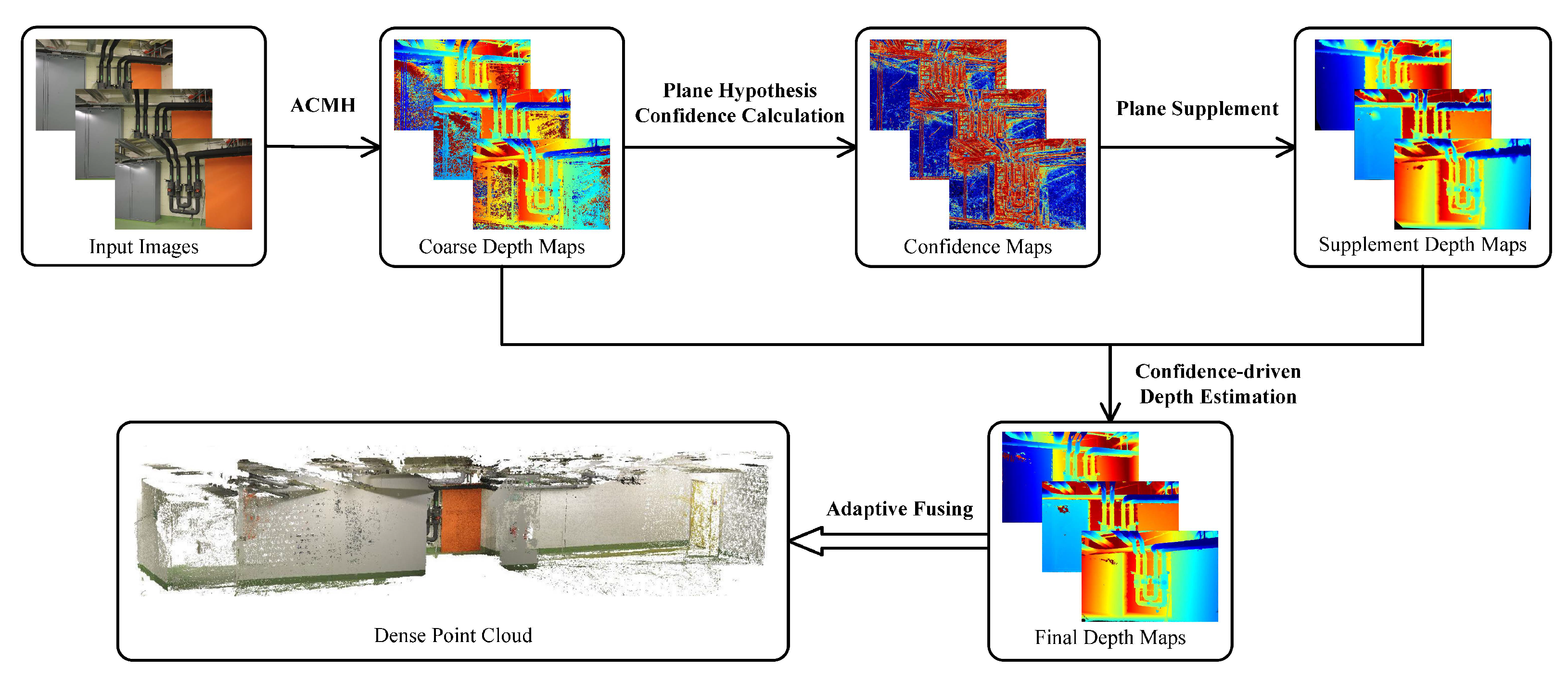
4.2. Plane Hypothesis Confidence Calculation

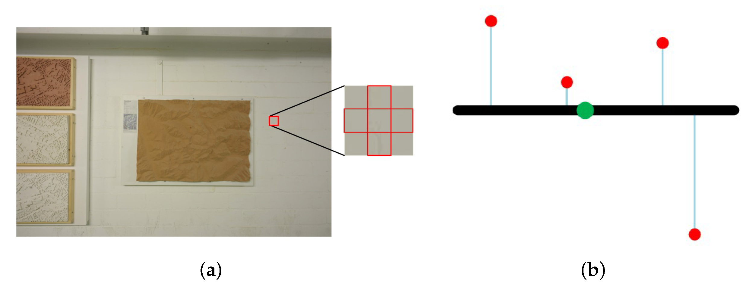
During the original depth estimation, photometric consistency appears as the problem of fuzzy matching in weakly textured regions. The problem is demonstrated by the fact that the depth of the incorrect plane hypothesis can make it possible to match highly similar regions between multiple views, making the multiview matching cost lack credibility. Ref. [15] attempts to add geometric consistency constraints to the multiview matching cost to reduce the erroneous plane hypotheses in weakly textured regions. Ref. [31] tries to add local consistency constraints to eliminate incorrect plane hypotheses.

However, photometric consistency would perfectly characterize the structure of the objects or scenes in structured scenes. Adding constraints to the matching cost certainly allows the fuzzy matching problem that occurs in weakly textured regions to be solved to some extent. However, the new constraints may blur the geometric details in the object or scene.

In contrast, we would like to capture which plane hypotheses are accurate enough to be represented the real objects or scenes after each depth estimate. Therefore, we propose a new confidence calculation method. The confidence expresses the degree of reliability of each plane hypothesis. For the plane hypothesis with large confidence, we consider that the plane hypothesis would accurately indicate the real surface of the scene or object. The plane hypothesis with low confidence is considered to be an incorrect estimation, and these incorrect plane hypotheses need to be filtered or upgraded. In the confidence calculation, the confidence is divided into two parts, including the multiview confidence and the patch confidence.

In multiview stereo, an assumption is that a reliable plane hypothesis should be geometrically stable between multiple views. Thus, based on the relationship of multiple views, a measure of multiview confidence is established firstly, which means the consistency degree of plane hypotheses among multiple views.

Note that the multiview confidence is calculated based on all neighboring views. The component of multiview confidence, which is calculated between the current view and one neighboring view, is defined as the view confidence.

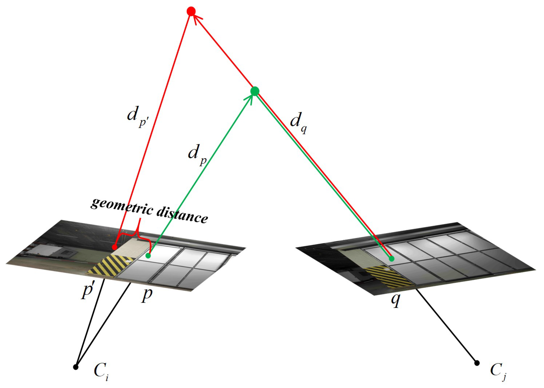
Given a pixel p, its plane hypothesis ${\varphi }_p$ is $(d_p,n_p)$. The multiview geometry is obtained as shown in Figure 3. The camera projection matrix from the current view $V_i$ to the neighboring view $V_j$ is calculated according to $d_p$. The pixel p is projected into the neighboring view $V_j$ to obtain the projected pixel q, and the plane hypothesis ${\varphi }_q$ of q would be obtained in the neighboring view. The pixel q is reprojected back into the current view to obtain the reprojection point $p^{\prime }$ according to the camera projection matrix from the neighboring view to the current view, which is calculated with $d_q$. By reprojecting the point $p^{\prime }$, the plane hypothesis ${\varphi }_{p^{\prime }}$ of $p^{\prime }$ corresponding to the current view $V_i$ can be obtained.

The view relationship between the current view and j-th neighboring view can be described via the reprojection distance ${\xi }_{geo}$, depth relative error ${\xi }_d$, normal pinch error ${\xi }_n$, and the matching cost $m\left({\varphi }_p,j\right)$. Therefore, ${\xi }_{geo}$, ${\xi }_d$, ${\xi }_n$ is calculated according to the pixel p, $p^{\prime }$ and the plane hypothesis $(d_p,n_p)$, $(d_{p^{\prime }},n_{p^{\prime }})$. Then, the view confidence consists of the geometric confidence $C_{geo}$, the depth confidence $C_d$, the normal confidence $C_n$, and the cost confidence $C_c$, which are calculated via the Gaussian function,

$$C_{geo}=e^{-\frac{{\xi }_{geo}^2}{2{\sigma }_{geo}^2}}=e^{-\frac{{\left(∥x_p-x_{p^{\prime }}∥\right)}^2}{2{\sigma }_{geo}^2}}$$

(7)

$$C_d=e^{-\frac{{\xi }_d^2}{2{\sigma }_d^2}}=e^{-\frac{1}{2{\sigma }_d^2}{\left[\frac{\left(d_p-d_{p^{\prime }}\right)}{d_p}\right]}^2}$$

(8)

$$C_n=e^{-\frac{{\xi }_n^2}{2{\sigma }_n^2}}=e^{-\frac{{\left[arccos\left(n_p·n_{p^{\prime }}\right)\right]}^2}{2{\sigma }_n^2}}$$

(9)

$$C_c=e^{-\frac{{m\left({\varphi }_p,j\right)}^2}{2{\sigma }_c^2}}$$

(10)

where ${\sigma }_{geo}$, ${\sigma }_d$, ${\sigma }_n$ and ${\sigma }_c$ are constants in the $C_{geo}$, $C_d$, $C_n$ and $C_c$, respectively.

In a set of neighboring views $\mathcal{V}=\left\{V_j|j=1,2,...,J\right\}$, there exist J sets of confidence relations for neighboring view. The multiview confidence is calculated as the average of the view confidence with all neighboring views:

$${\overline{C}}_g=\frac{{\displaystyle \sum _{j=1}^J}\left(C_{geo}^j·C_d^j·C_n^j·C_c^j\right)}{J}$$

(11)

A good plane hypothesis should be supported by multiple neighboring views. When the number of neighboring views that maintain consistency is increased, the trustworthiness of the planar hypothesis is improved. Meanwhile, the geometric stability in multiple views is increased. However, the camera’s pose variation and the presence of occlusion determine that not all regions in a view can be consistent with multiple views. Specifically, some regions in a view are only visible in a limited number of neighboring views. Thus, in these regions, calculating the view confidence with all neighboring views may cause the correct plane hypothesis to be judged as unreliable. To this end, the multiview confidence calculation is modified to be the average of the best K neighboring views among all neighboring views.

$$C_g=\frac{{\displaystyle \sum _{j=1}^K}\left(C_{geo}^j·C_d^j·C_n^j·C_c^j\right)}{K}$$

(12)

The global spatial information is fully considered in the multiview confidence, which is based on the consistency of multiple measurements. The multiview confidence calculation makes most plane hypotheses easy to calculate as reliable estimates with high confidence. However, for some plane hypotheses that are correctly estimated in current view, erroneous multiview confidences are calculated because of wrong plane hypotheses in neighboring views. In addition, because of similar plane hypotheses in multiple views, some noise in the current view may be calculated as high-confidence and retained, especially in weakly textured regions.

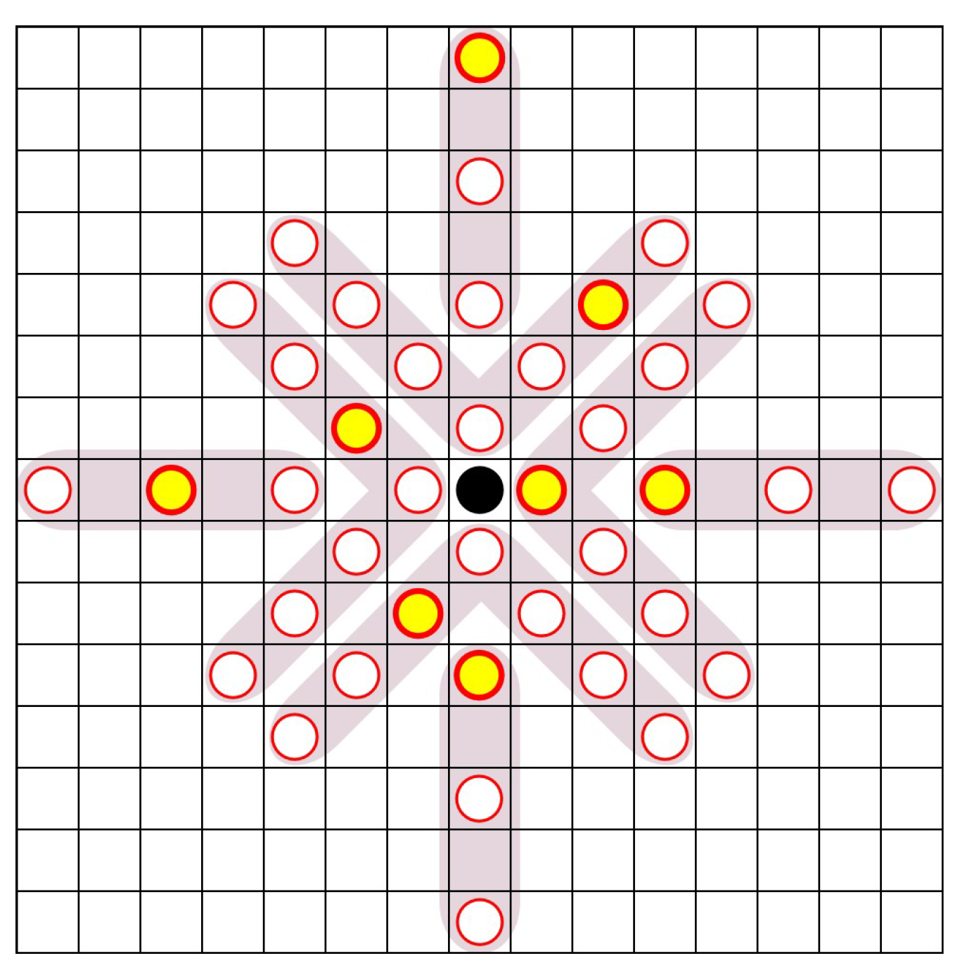
In order to reduce the calculation of error confidence, a patch confidence measure based on depth local consistency is added, which only relies on the information in the current view. In the PatchMatch algorithm [5,45], a key statement is that relatively large regions of pixels can be modeled by an approximately 3D plane. It allows the same plane hypotheses to be shared within the pixel regions. The statement can be beneficial to help exploit the local information in a view. To this end, the patch confidence is structured as a calculation based on the consistency of local planes. For each pixel in the current view, a cruciform patch is constructed, centered on the pixel. Firstly, a 3D local plane is constructed in the camera coordinate via the central pixel’s 3D point $X_c$ and its corresponding plane hypothesis. Secondly, neighboring pixels in a cruciform patch are projected into the same camera coordinate to obtain 3D points $X_n$. The average Euclidean distance from the 3D points of neighboring pixels to the local 3D plane is calculated (refer to Figure 4),

$$\overline{\xi }=\frac{1}{N}·{\displaystyle \sum _{n=1}^N}{\xi }_n=\frac{1}{N}·{\displaystyle \sum _{n=1}^N}\frac{n_c·\left(X_c-X_n\right)}{\sqrt{n_{cx}^2+n_{cy}^2+n_{cz}^2}}$$

(13)

where N is the number of pixels in a cruciform patch and $n_c$ is the normal of patch center pixel. $n_{cx}$, $n_{cy}$, $n_{cz}$ are the three components of normal $n_c$.

Based on the calculated average Euclidean distance, patch confidence is constructed by the Gaussian function as well:

$$C_l=e^{-\frac{{{}^{\overline{\xi }}}^2}{2{\sigma }_p^2}}$$

(14)

where ${\sigma }_p$ is a constant parameter of patch confidence.

Finally, via the calculated multiview confidence and patch confidence, the confidence of the pixel p can be expressed as

$$C\left(p,{\varphi }_p\right)=C_g·C_l$$

(15)

4.3. Plane Supplement and Confidence-Driven Depth Estimation

The purpose of the propagation scheme is that the reasonable plane hypotheses can be propagated to other pixels in the same plane, making the estimation accurate and reliable. However, in the weakly textured regions, it is difficult to select the correct plane hypothesis using the matching cost function based on luminosity consistency, because the weakly textured regions usually do not contain discriminative information. This makes it difficult for incorrect plane hypotheses to be replaced by correct neighborhood candidate planes via the propagation scheme, and these incorrect plane hypotheses may be propagated to other pixels due to the propagation scheme.

This means that relying on existing plane hypotheses cannot help the reconstruction of weakly textured regions. Ref. [18] chooses the base point via photometric consistency cost to generate the prior plane and introduces them into the calculation of multiview matching cost. However, the photometric consistency is not reliable in weakly textured regions, giving prior planes wrong plane hypotheses. In addition, the photometric consistency cost of incorrect planar hypothesis may be sufficiently small in weakly textured regions. Despite using prior planes as a constraint in the calculation of multiview matching cost, it does not allow these errors to recompute an aggregation cost large enough to be replaced by correct plane hypotheses contained in prior planes. It keeps the wrong plane hypotheses in weakly textured regions of depth maps.

In Section 4.2, the confidence is proposed to discriminate the accuracy and reliability of plane hypotheses to avoid misjudgment of photometric consistency in weakly textured regions. After the plane hypothesis confidence calculation, pixels with high confidence (we set the confidence threshold ${\delta }_c$ to 0.8) are extracted from the coarse depth map. The key observation behind this is that these pixels with high confidence mostly contain the structure of 3D scenes. Meanwhile, the planar hypotheses of extracted pixels are accurate and reliable, because they are supported by multiple views and are consistent in local planes. Using the extracted pixels as base points, the images are divided into multiple triangular primitives with different sizes using Delaunay triangulation [46]. Then, based on the depths of the three base points in the triangular primitives, a local 3D plane where the triangular primitives are located is constructed. For the low-confidence pixels contained in each triangular primitive, they are projected into the local 3D plane to obtain new depths, resulting in additional supplemental depth maps.

The supplemental planes perform well in weakly textured regions, especially those with large planes. However, some edge regions are blurred, which is contrary to photometric consistency. The coarse depth map that depends on photometric consistency is calculated with higher confidence than the supplemental depth map in these edge regions. Conversely, the confidence of the supplemental depth map is better than the coarse depth map in weakly textured regions.

Thus, the coarse depth map and supplemental depth map are jointly fed to a comparison module. Specifically, after obtaining the supplemental depth maps, the plane hypothesis confidence calculation module is reapplied to calculate the confidence for each plane hypothesis in the supplemental depth map. The confidences calculated in the supplemental depth map are compared with the coarse depth map, and the planar hypotheses with higher confidence are retained.

Subsequently, the retained plane hypotheses are used as the initial values for the confidence-driven depth estimation. An important reason for confidence-driven depth estimation is that there are still some erroneous plane hypotheses mixed in with the retained plane hypotheses. These noises tend to exhibit low confidence in both the supplemental depth maps and the coarse depth maps. These noises can be effectively reduced with the help of the propagation mechanism and the modified cost function. The results obtained by combining the supplemental depth maps and the coarse depth maps lose partial structural details. Since the photometric consistency cost has a significant result in textured regions, it is possible to exploit this advantage to help the recuperation of these textured regions. In addition, plane supplementation has a significant recovery for planar surfaces in weakly textured regions. However, there is a subtle variation in the plane hypotheses in curved surfaces of weakly textured regions, which causes a slight decrease in the accuracy of our plane supplement. The propagation step and the refinement step in the depth estimation can effectively help these curved surfaces to produce the correct variations of plane hypotheses instead of keeping them in the same plane.

In the confidence-driven depth estimation, the processes of propagation and refinement are kept in line with the ACMH [22], which are reviewed in Section 3. In particular, for the multiview matching cost calculation, confidence is used as a constraint to limit the propagation of incorrect plane hypotheses with low confidence to other pixels. Meanwhile, planar hypotheses with high confidence can be easily propagated to other pixels of the same plane with the help of the propagation scheme. According to the Equation (6), the confidence-driven multiview matching cost function is modeled as

$$m\left(p,{\varphi }_p\right)=\frac{{\displaystyle \sum _{j=1}^{N-1}}{w^{\prime }}_j·m\left({\varphi }_p,j\right)+\lambda ·\left(1-C\left(p,{\varphi }_p\right)\right)}{{\displaystyle \sum _{j=1}^{N-1}}{w^{\prime }}_j}$$

(16)

where $C\left(p,{\varphi }_p\right)$ is the confidence of pixel p, which is calculated with the plane hypothesis ${\varphi }_p$, and $\lambda$ is a weight constant.

For weakly textured regions, the matching cost of photometric consistency computed by different plane hypotheses is usually similar because of the lack of distinguishability information. It causes the propagation mechanism in traditional MVS to easily transmit erroneous plane hypotheses to other pixels in these regions, and is difficult to replace. According to the modified confidence-driven multiview matching cost, the determining factor for propagation mechanism to judge the reliability of the candidate plane hypotheses is confidence. Because the confidence level calculated in the noise is small, the multiview matching cost calculated in the noise is larger than the correct plane hypothesis. Thus, the confidence-driven multiview matching cost would be helpful to address the problem of propagation mechanism for candidate plane hypothesis selection. Meanwhile, plane hypotheses with high confidence can be easily transmitted to pixels in the same plane because they are computed at a low cost. For the structural detail regions, the important factor that dominates the propagation mechanism’s selection of candidate plane hypotheses changes to the photometric consistency matching cost. The reason is that the calculated confidences are all great in these regions. Thus, the detail regions that were previously blurred and erroneous would be improved.

To avoid the complexity of repeated confidence calculations due to changes in plane hypotheses, the confidence-driven depth estimation is restricted to obtaining the final depth maps with one propagation. Via this confidence-driven depth estimation, the final depth maps preserve the structural details well and improve the estimation quality of weakly textured regions.

4.4. Adaptive Fusion

After depth estimation, all the depth maps of views are obtained. In the depth map fusion step, all the depth maps are merged into the dense point clouds. In [6,7], all the depth maps are fused by consistent matching with a fixed threshold. Specifically, for each pixel, it is projected into each neighboring view via its depth of plane hypothesis. Then, it is reprojected back to current view by the depth of hypothesis, which is in the neighboring view. The corresponding matching relationship can be obtained based on the reprojected point and the pixel in the current view. A consistent matching is defined as satisfying the consistent constraints, including depth difference ${\delta }_d\le 0.01$ and normal angle ${\delta }_n\le 10$. For all neighboring views, if there exist $n\ge \delta$ neighboring views (defining $\delta$ as the view constraint) satisfying the consistent matching, the hypothesis is accepted. Finally, all pixels that satisfy the consistency matching are projected into the 3D space and averaged into uniform 3D points, thus becoming part of the dense 3D point clouds. Refs. [15,18,22] further tighten the consistent constraints of consistency matching on this depth fusion approach; the reprojection geometry error ${\delta }_{geo}\le 2$ should be satisfied.

However, we observe that such a depth map fusion approach relies on fixed consistent constraints and fixed view constrain. There are always situations where some regions of the current view are only visible in a limited number of neighboring views. Then, too large a view constraint will cause these regions cannot to be fused into the dense point clouds, resulting in a lack of completeness. Too small a view constraint ensures the fusion of these areas, but leads to a decrease in the overall reconstruction quality, especially in terms of accuracy.

To solve this problem, an adaptive depth fusion approach is developed. Specifically, the view weight is added to each neighboring view when calculating the multiview matching cost. Such view weights can reflect the visibility relationships of pixels in multiple views. At the end of the last depth estimation, the view weights corresponding to all neighboring views of all pixels are retained. In the depth map fusion step, firstly, all neighborhood view weights corresponding to each pixel are sorted from large to small. Secondly, based on the distribution changes of neighborhood view weights, the view constraints $\delta \left(V_i\right)$ can be adjusted adaptively.

$$\delta \left(V_i\right)=\left\{\begin{array}{cc}j,\hfill & {w^{\prime }}_j>{\delta }_w\cap {w^{\prime }}_j<{\delta }_w\cap j\le 4;\hfill \\ 4\hfill & j>4.\hfill \end{array}\right.$$

(17)

where ${w^{\prime }}_j$ denotes the j-th sorted view weight of neighboring views. ${\delta }_w$ is the threshold of the view weight. After sorting, the comparison starts from the largest neighborhood view weight to the threshold of view weight. For the view weight ${w^{\prime }}_j\ge {\delta }_w$, we consider the pixel to be visible in corresponding neighboring view. The view constraint is adaptively adjusted to the number of neighboring views accumulated. Until the j-th view weight ${w^{\prime }}_j\le {\delta }_w$, we consider that the pixel’s visibility starts to be insufficient. In addition, the main goal of our adaptive fusion is to ensure accuracy while improving the integrity of invisible regions. The increase in view constraint indicates that the visibility of the regions is satisfied in multiple neighborhood views, but it becomes difficult to satisfy the consistency of plane hypotheses between multiple views. To prevent the influence of excessive view constraint on the completeness of these regions, the view constraint is phased at the maximum value of 4.

Simultaneously, to ensure as much as possible that the adaptive view constraints are adjusted by visibility judgments rather than resulting in incorrect plane hypotheses, the consistency constraints of consistent matching are adaptively adjusted according to the size of the view constraint. For pixels with small view constraints, the consistency constraints are tightened to ensure that their plane hypotheses are accurate enough. For pixels with large view constraints, the consistency constraints are relaxed appropriately, allowing the pixels supported via multiple neighboring views to be easily merged into point clouds to improve the completeness of reconstruction.

$${\delta }_d^{new}=\left[ln\left(2·\delta \left(V_i\right)-1\right)+1\right]·{\delta }_d$$

(18)

$${\delta }_n^{new}=\left[ln\left(2·\delta \left(V_i\right)-1\right)+1\right]·{\delta }_n$$

(19)

$${\delta }_{geo}^{new}=\left[ln\left(2·\delta \left(V_i\right)-1\right)+1\right]·{\delta }_{geo}$$

(20)

where ${\delta }_d$, ${\delta }_n$, ${\delta }_{geo}$ is the strictest consistency constraint when the view constraint $\delta \left(V_i\right)$ is 1. With the view constraint increased, the consistency constraints become loose, making pixels easy to be merged into dense point clouds when they are visible among multiple views.

In addition, for outdoor scenes, the sky regions become redundant in the dense point clouds, because the sky regions lack true depth. Through a guided-filter-based mask refinement method, Ref. [47] uses a neural network and weighted guided upsampling to create accurate sky alpha masks at high resolution, resulting in the segmentation of sky regions. Thus, before the beginning of the depth fusion step, the method in [47] is applied to filter out the plane hypotheses of sky regions contained in the depth maps. The sky-filtering step has almost no effect on the calculation of the quantifiers. However, we can obtain clean depth maps as well as dense point clouds.

With the depth map fusion approach described above, we can obtain dense 3D point clouds with high completeness and accuracy.

5. Experiments

The proposed CGPR-MVS is implemented in C++ with CUDA. To evaluate the proposed pipeline, we perform quantitative and qualitative evaluations on the published dataset ETH3D benchmark [48]. In addition, the qualitative evaluation is performed on the sensefly dataset. The experiments were conducted on a machine equipped with Intel Xeon E5-1630 v4 CPU, 64G RAM, and NVIDIA Quadro K2200 GPU.

The ETH3D benchmark contains both high-resolution datasets and low-resolution datasets for the MVS task. Further, the high-resolution dataset is divided into the training branch and the test branch, with all images having a resolution of 6048 × 4032. The training branch dataset contains 13 sequences of indoor and outdoor scenes, with additional ground truth point clouds and ground truth depth maps. The test branch dataset contains 12 sequences of indoor and outdoor scenes, and the evaluation is only available by uploading to the online website, and the ground truth data are not publicly available. During the evaluation, the quality of the reconstruction results is quantified in three metrics as accuracy, completeness, and $F_1$ score. The accuracy is the percent fraction of the reconstruction, which is closer to the ground truth than the evaluation tolerance. The completeness is the percent fraction of the ground truth, which is closer to the reconstruction than the evaluation tolerance. The $F_1$ score is the harmonic mean of accuracy and completeness. For details of the whole evaluation, please refer to [48].

The sensefly datasets are collected from real remote sensing images captured by various drones with different cameras from AgEagle, a company that provides fixed-winged drones and aerial imagery-based data collection and analytics solutions. The datasets contain several different scenes, each with different flight heights and applied in different practical applications. A challenging scene is selected to test in our experiment. The dataset of Thammasat University campus in Bangkok, Thailand was collected by an eBee X drone carrying an Aeria X photogrammetry camera. The drone flew at a height of 285 m, photographed scenes covering 2.1 square kilometers, and captured high-resolution images of 6000 × 4000. Usually, these collected datasets are used for 3D mapping, regular updating of city maps, inspecting infrastructure, monitoring construction projects, and studying architectural aspects.

5.1. Parameter Settings

Firstly, the undistorted images are downsampled to the resolution of 3200 × 2130 for reconstruction. For all datasets, the same set of parameters is used in the experiments. The specific parameter settings are shown in

Table 1. Parameter settings of experiments and their meaning.

Parameter	Meaning	Value
${\sigma }_{geo}$	constant of geometric confidence	$5.0$
${\sigma }_d$	constant of depth confidence	$0.05$
${\sigma }_n$	constant of normal confidence	$0.8$
${\sigma }_c$	constant of cost confidence	$0.5$
K	best K neighboring views	2
${\sigma }_p$	constant of patch confidence	$1.0$
${\delta }_c$	confidence threshold	$0.8$
$\lambda$	constant of confidence constraint in multiview matching cost	$2.0$
${\delta }_w$	threshold of view weight	$0.6$
${\delta }_d$	the strictest depth difference	$0.01$
${\delta }_n$	the strictest normal angle	$0.15$
${\delta }_{geo}$	the strictest geometry error	$1.5$

.

5.2. Quantification

Some state-of-the-art MVS methods and our method were compared by quantitative evaluation on the high-resolution of ETH3D benchmark, including Gipuma [10], COLMAP [15], ACMH [22], OpenMVS [7], ACMP [18], CLD-MVS [38], QAPM [21]. The quantitative evaluation performance of the training branch dataset and the test branch dataset are shown in

Table 2. Quantitative evaluation comparative results ($F_1$ score, accuracy, completeness) at default tolerance of 2 cm on high-resolution training dataset of ETH3D benchmark.

Method		All			Indoor			Outdoor
	${\mathit{F}}_1$	Acc.	Comp.	${\mathit{F}}_1$	Acc.	Comp.	${\mathit{F}}_1$	Acc.	Comp.
Gipuma [10]	36.38	86.47	24.91	35.80	89.25	24.61	37.07	83.23	25.26
COLMAP [15]	67.66	91.85	55.13	66.76	95.01	52.90	68.70	88.16	57.73
ACMH [22]	70.71	88.94	61.59	70.00	92.62	59.22	71.54	84.65	64.36
OpenMVS [7]	76.15	78.44	74.92	76.82	81.39	73.91	75.37	74.99	76.09
ACMP [18]	79.79	90.12	72.15	80.53	92.30	72.25	78.94	87.58	72.03
CLD-MVS [38]	79.35	82.75	77.36	81.23	87.22	77.29	77.16	77.54	77.45
QAPM [21]	78.47	80.43	77.50	80.22	84.34	77.43	76.43	75.86	77.59
OURS	82.64	86.66	79.39	85.03	88.52	82.13	79.86	84.48	76.19

The best results are marked in bold black.

and

Table 3. Quantitative evaluation comparative results ($F_1$ score, accuracy, completeness) at default tolerance of 2 cm on high-resolution test dataset of ETH3D benchmark.

Method		All			Indoor			Outdoor
	${\mathit{F}}_1$	Acc.	Comp.	${\mathit{F}}_1$	Acc.	Comp.	${\mathit{F}}_1$	Acc.	Comp.
Gipuma [10]	45.18	84.44	34.91	41.86	86.33	31.44	55.16	78.78	45.30
COLMAP [15]	73.01	91.97	62.98	70.41	91.95	59.65	80.81	92.04	72.98
ACMH [22]	75.89	89.34	68.62	73.93	91.14	64.81	81.77	83.96	80.03
OpenMVS [7]	79.77	81.98	78.54	78.33	82.00	75.92	84.09	81.93	86.41
ACMP [18]	81.51	90.54	75.58	80.57	90.60	74.23	84.36	90.35	79.62
CLD-MVS [38]	82.31	83.18	82.73	81.65	82.64	82.35	84.29	84.79	83.86
QAPM [21]	80.88	82.59	79.95	79.50	82.59	77.39	85.03	82.58	87.64
OURS	85.76	86.17	85.71	85.29	85.54	85.46	87.17	88.05	86.46

The best results are marked in bold black.

respectively. Note that the evaluation tolerance is 2 cm, as defaulted by the ETH3D benchmark. The quantitative evaluation of other approaches is dependent on the published results on the online website of the ETH3D benchmark.

As shown in Table 2, the proposed method achieves the best performance of $F_1$ score and completeness compared with other methods in the training branch dataset, except for outdoor scenes, where completeness is slightly inferior to QAPM. The main contribution of Gipuma is the parallelized red–black checkerboard propagation, which brings a huge improvement in the efficiency of depth estimation. However, its performance is far inferior to other schemes in the quality of reconstruction, because it simply selects the top-k minimum matching cost for averaging to represent the multiview matching cost. Both COLMAP and ACMH are based on the matching cost of photometric consistency. It makes them suffer from fuzzy matching problems in weakly textured regions and perform poorly in completeness, which in turn affects the $F_1$ score. On the contrary, they possess an extremely high accuracy attributed to their contribution to view selection strategy and the check of geometric consistency. OpenMVS also uses the matching cost based on photometric consistency. By relaxing the view constraint on depth fusion, it performs poorly in terms of accuracy, but the increase in completeness results in an improvement in the $F_1$ score. ACMP introduces planar priors to improve completeness. However, the generation of planar priors relies excessively on the multiview matching cost based on photometric consistency, which allows erroneous planar priors to be generated and mislead the computation of the improved cost function. CLD-MVS utilizes a boundary-aware interpolation method, which improves completeness while decreasing its accuracy, and it results in an inferior performance to our method. QAPM extracts pixel information with the same plane by constructing the quadtree, then the plane priors are generated by a plane fitting algorithm. However, the plane fitting algorithm is not implemented completely for all quadtree blocks, which leads to a lot of vacancies in the generated prior planes. In addition, nearly but not sufficiently accurate prior planes would affect the accuracy of the reconstruction. The great success in completeness makes our method ahead of other SOTA methods in the $F_1$ score, while the accuracy is not overly behind the most accurate method COLMAP. The improvement in completeness is attributed to the fact that after utilizing the confidence calculation method, the supplemental depth maps are generated based on it and combined with the coarse depth maps. It allows for an effective recovery of weakly textured regions, especially those planes in weakly textured regions, without blurring the structural detail regions.

The performance of the proposed method is further demonstrated by the comparison results of the test branch dataset shown in Table 3. Except for the outdoor scenes, where the completeness is slightly inferior to QAPM, our method ranks first in both completeness and $F_1$ score. In addition, the comparison results of different scenes in the test branch dataset at different distance tolerances are shown in Figure 5. It can be seen that our method almost achieves the most competitive f1 scores for different sequences at each distance tolerance, except for the ’exhibition hall’ sequence. It means that our method is robust for different scene sequences, although at different evaluation tolerances. In addition, the accuracy requirements for the reconstructed point clouds vary greatly in practical applications, which gives all of the reconstruction results for different thresholds a reference significance of comparison. Through the comparison between different sequences, it can be seen that while the scenes contain a lot of weakly textured planes, our method achieves excellent results for resolving the problems of luminosity consistency in these regions, resulting in the most competitive $F_1$ score. The ’lounge’ scene sequence is noteworthy among them all. The ’lounge’ sequence is the one scene where all methods perform poorly because of the presence of large reflective floor areas in this indoor scene. It causes a failure in photometric consistency and makes depth estimation difficult. An important reason for the best competitiveness of our method in this sequence is the proposed confidence calculation method, then the planar supplement based on our confidence. ACMP and QAPM are both planar-based methods, but their planar generation is based on photometric consistency, which makes them perform worse than us on this sequence. The interpolation method of CLD-MVS blurs the geometric details and results in reduced accuracy, which also affects the $F_1$ score. In contrast, we perform plane supplementation and then combine the supplemental depth maps with the coarse depth maps, which effectively improves the deficiency of plane supplementation in geometric detail regions and provides reliable planes in weakly textured regions.

5.3. Qualification

The qualitative evaluation is compared with some state-of-the-art PatchMatch-based MVS methods in terms of both depth maps as well as dense point clouds. For the ETH3D benchmark, all the dense point clouds are obtained from the results submitted on the online website to fairly compare the reconstruction quality of all methods. The depth map results with other methods are implemented in our machine via their open-source code. For the sensefly dataset, both the dense point clouds and the depth map results are implemented through open-source code.

For partial sequences of the ETH3D benchmark’s high-resolution dataset, the comparison of qualitative depth maps is shown in Figure 6. The challenges in the ETH3D benchmark arise from a huge variation in camera angles between different images and the magnification of weakly textured regions in the high-resolution images, while the former leads to an increase in occlusion. The second aggravates the difficulty of reconstruction of weakly textured regions, because the images in the benchmark contain a large number of weakly textured surfaces (e.g., walls, floors, roads, ceilings). It can be seen that the depth maps of OpenMVS and ACMH contain a large amount of noise, and these incorrectly estimated depths are detrimental to both accuracy and completeness. COLMAP also contains a lot of noise; most of the noise is filtered out after the geometric consistency check, resulting in accurate but extremely incomplete depth maps. ACMP improves the quality of the depth maps via the plane priors. However, it is inferior to the depth maps of our method, which is due to the generation of prior planes relying on the cost function of photometric consistency. In contrast, the proposed confidence calculation would address well the unreliability of photometric consistency in weakly textured regions. Thus, the depth maps with high quality are estimated in combination with the plane supplement module.

A comparison of the qualitative depth maps for the university scene of the sensefly dataset is shown in Figure 7. The challenges of the sensefly dataset are the poor overlap of the images and the absence of common viewing areas. In addition, the weakly textured regions in these remote sensing images are mostly concentrated on roads and building roofs. As shown in Figure 7, the depth map of the COLMAP exhibits large vacancies. Besides the weakly textured regions that fail to estimate the correct depths, the poor overlap of the images leads to the misuse of geometric consistency in the COLMAP. The reason is that some regions are invisible in partial—or even all—neighborhood views. This removes the depth of these regions in the geometric consistency check, resulting in large vacancies. OpenMVS and ACMH still perform poorly in the weakly textured planes, while ACMP improves. In contrast, the depth maps of our method are most intact in these planar regions, which indicates the successful recovery of our method in the weakly textured planes.

Through the proposed adaptive depth fusion approach, the obtained dense point clouds are compared with other MVS methods. For the high-resolution training and test datasets of the ETH3D benchmark, qualitative comparisons of the dense point clouds for some sequences are shown in Figure 8 and Figure 9, respectively. It can be seen that COLMAP and ACMH exhibit large vacancies in weakly textured regions, which makes their point clouds sparse. OpenMVS, which also utilizes the photometric consistency matching cost, sacrifices significant accuracy for an increase in completeness by decreasing the view constraint in depth fusion. Therefore, the point clouds of OpenMVS seem to be dense. However, they contain a lot of redundancy, which severely reduces the accuracy of the point clouds. The planar priors of ACMP bring a great improvement in completeness while maintaining high accuracy. However, it can be seen that the point cloud still appears sparse and vacant in weakly textured regions, especially in weakly textured planar surfaces. This is due to the incorrect prior planes generated in these regions, which are guided by the matching cost of photometric consistency. In contrast, our method recovers completely in these regions, especially in indoor scenes, which usually contain more weakly textured planar surfaces (e.g., walls, floors). Due to the effect of adaptive fusion, although the regions with insufficient visibility are effectively recovered in dense point clouds, some erroneous redundancies inevitably appear. These redundancies are one reason why the accuracy of our quantitative evaluation does not outperform other methods. However, the slight decrease in accuracy is worth it compared to our great improvement in completeness.

In addition, the comparison of point clouds on the sensefly dataset is shown in Figure 10. It can be seen that the point clouds reconstructed by COLMAP and ACMH are both sparse. ACMP has a better reconstruction in the weakly textured regions, but the overall denseness is not as good as that of OpenMVS and ours. The point clouds of OpenMVS, which are only based on the photometric consistency, show the densest point clouds in the comparison. An important reason for the above observation is attributed to the difference in depth fusion methods. COLMAP, ACMH, and ACMP all require a high view constraint for depth fusion, which makes their reconstructed point clouds sparse, although ACMP performs well in depth maps. In contrast, OpenMVS uses the most relaxed view constraint for depth fusion, which results in the densest reconstructed point clouds. Our adaptive fusion method dynamically adjusts the view constraint, which results in a far denser point cloud than COLMAP, ACMH, and ACMP, but slightly sparser than OpenMVS. However, the advantage of our method is that the reconstruction is more integral in the weakly textured regions, especially the planar surfaces of these regions, such as the building roofs and the water surface shown in the red box of Figure 10.

To further illustrate the effectiveness of our pipeline in weakly textured regions, the comparison results of completeness visualizations are shown individually in Figure 11. The completeness visualizations are provided on the online website of the ETH3D benchmark and are only available in the training branch dataset. It can be clearly seen that the results of our method have more green parts (meaning the parts that are reconstructed successfully) of point clouds compared to other methods. Most of the green parts of point clouds belong to weakly textured regions. For the successful recovery in weakly textured regions, our method can outperform other methods in terms of completeness.

5.4. Ablation Study

To evaluate the effectiveness of each part of our proposed method, we conducted ablation experiments on the high-resolution training dataset of the ETH3D benchmark. The evaluation results are presented in

Table 4. Ablation study results ($F_1$ score, accuracy, completeness) at default tolerance of 2 cm on high-resolution training dataset of ETH3D benchmark.

Method	${\mathit{F}}_1$ Score	Accuracy	Completeness
Baseline	72.77	90.65	62.46
CGPR-MVS/C	74.40	76.59	73.70
CGPR-MVS/S	78.41	85.68	73.40
CGPR-MVS/A	79.71	90.72	71.87
CGPR-MVS	82.64	86.66	79.39

The best results are marked in bold black.

. In the table, we list the results of removing different modules from our proposed CGPR-MVS, including without all modules proposed (baseline), without confidence calculation (CGPR-MVS/C), without plane supplement (CGPR-MVS/S), without adaptive fusing (CGPR-MVS/A), and the whole pipeline in CGPR-MVS. For CGPR-MVS/C, we use the matching cost as a substitute for completing the plane supplement module. For CGPR-MVS/S, we filter the unreliable estimation by confidence after the confidence is computed in the confidence calculation module. For CGPR-MVS/A, we set fixed-view constraint and fixed-consistency constraints for depth fusion, like other pipelines [7,15,18,22].

Firstly, a quantitative comparison between CGPR-MVS and CGPR-MVS/A shows that the adaptive fusion approach greatly balances the accuracy and completeness of the reconstruction results. After removing adaptive fusion, the pipeline achieves extremely high accuracy. Nonetheless, both accuracy and completeness are increased compared to the baseline method. In CGPR-MVS/C, the proposed confidence calculation is replaced by the multiview matching cost of photometric consistency to help the subsequent implementation of the plane hypothesis supplement. By comparing CGPR-MVS and CGPR-MVS/C, the result without confidence calculation is that the completeness and accuracy of the quantitative evaluation are significantly reduced. The results further illustrate the failure of photometric consistency in the weakly textured regions, and prove that the proposed confidence calculation is extremely effective for the improvement in reconstruction quality. Compared to the quantitative evaluation results of CGPR-MVS and CGPR-MVS/S, there is essentially no excessive change in accuracy, but there is a significant decrease in completeness after removing the planar hypothesis supplement. Based on the implementation of confidence calculation, the planar hypothesis supplement provides reliable planar hypotheses for the weakly textured region, which helps converge to the global optimal solution. In contrast, after losing the planar hypothesis supplement, the plane hypotheses of weakly textured regions are limited to the wrong local optimal solution, resulting in the failure of reconstruction.

5.5. Time Evaluation

For each 3200 × 2130 resolution view in the high-resolution training dataset of the ETH3D benchmark, the runtimes of each proposed section and the total runtime are listed in

Table 5. Different modules’ running times for one image of 3200 × 2130 resolution on high-resolution training dataset of ETH3D benchmark.

Module	Time(s)	Ratio (%)
depth estimation of ACMH	18.79	49.70
plane hypothesis confidence calculation	2.36	6.24
plane supplement	3.52	9.31
confidence-driven depth estimation	13.14	34.75
Total	37.81	-

. It can be seen that both the plane hypothesis confidence calculation module and plane supplement module do not impose an excessive runtime burden for depth estimation. Moreover, since the machine configuration is not expensive, the runtime results show that the proposed pipeline can be equipped on low-performance machines without consuming excessive computational resources.

In addition, the comparison results between the proposed method and some GPU-based methods are shown in

Table 6. Comparison of running times for one image of 3200 × 2130 resolution on high-resolution training dataset of ETH3D benchmark.

Method	COLMAP	ACMM	ACMP	OURS
Time(s)	129.9	43.0	23.7	37.8

The best results are marked in bold black.

. The running times of all the methods are experimentally obtained on our machines equipped with a single GPU. It can be seen that even with the GPU, COLMAP [15] still has the longest running time, because of the sequential propagation in depth estimation. Our pipeline takes more time than ACMP [18], but still has a shorter running time than ACMM [22] and COLMAP [15]. The comparison results further show that the proposed method is efficient enough and does not require more computational resources.

6. Conclusions

In this work, we propose a novel MVS method, which is called confidence-guided planar recovering multiview stereo (CGPR-MVS). After depth estimation, the confidence calculation module is applied to depth maps to produce pixel-wise confidence, which contains multiview consistency and patch consistency. Based on the plane hypothesis confidence calculation, a Delaunay triangle-based plane supplement module additionally provides reliable plane information. The supplemental depth map and coarse depth map are fed into a confidence-driven depth estimation to achieve high-integrity recovery without losing the structural detail regions. Via adaptive fusion, invisible regions can be merged into dense point clouds. Qualitative and quantitative evaluations of high-resolution MVS datasets demonstrate the efficiency and effectiveness of our method, especially in the reconstruction quality of weakly textured planes. In future work, we will focus on improving the accuracy of texture detail regions while maintaining reconstruction completeness.

References

1. Xu, Z.; Liu, Y.; Shi, X.; Wang, Y.; Zheng, Y. MARMVS: Matching Ambiguity Reduced Multiple View Stereo for Efficient Large Scale Scene Reconstruction. In Proceedings of the 2020 IEEE/CVF Conference on Computer Vision and Pattern Recognition (CVPR), Seattle, WA, USA, 13–19 June 2020; pp. 5980–5989. [Google Scholar] [CrossRef]
2. Zhou, L.; Zhang, Z.; Jiang, H.; Sun, H.; Bao, H.; Zhang, G. DP-MVS: Detail Preserving Multi-View Surface Reconstruction of Large-Scale Scenes. Remote Sens. 2021, 13, 4569. [Google Scholar] [CrossRef]
3. Zhang, Q.; Luo, S.; Wang, L.; Feng, J. CNLPA-MVS: Coarse-Hypotheses Guided Non-Local PatchMatch Multi-View Stereo. J. Comput. Sci. Technol. 2021, 36, 572–587. [Google Scholar] [CrossRef]
4. Xu, Q.; Kong, W.; Tao, W.; Pollefeys, M. Multi-Scale Geometric Consistency Guided and Planar Prior Assisted Multi-View Stereo. IEEE Trans. Pattern Anal. Mach. Intell. 2023, 45, 4945–4963. [Google Scholar] [CrossRef] [PubMed]
5. Bleyer, M.; Rhemann, C.; Rother, C. PatchMatch Stereo-Stereo Matching with Slanted Support Windows. In Proceedings of the British Machine Vision Conference (BMVC), Dundee, UK, 29 August–2 September 2011; pp. 14.1–14.11. [Google Scholar] [CrossRef]
6. Shen, S. Accurate Multiple View 3D Reconstruction Using Patch-Based Stereo for Large-Scale Scenes. IEEE Trans. Image Process. 2013, 22, 1901–1914. [Google Scholar] [CrossRef] [PubMed]
7. Cernea, D. OpenMVS: Multi-View Stereo Reconstruction Library. Available online: https://cdcseacave.github.io/openMVS (accessed on 4 August 2022).
8. Fuhrmann, S.; Langguth, F.; Goesele, M. MVE—A Multi-View Reconstruction Environment. In Proceedings of the Eurographics Workshop on Graphics & Cultural Heritage, Darmstadt, Germany, 6–8 October 2014. [Google Scholar]
9. Zhu, Z.; Stamatopoulos, C.; Fraser, C.S. Accurate and occlusion-robust multi-view stereo. ISPRS J. Photogramm. Remote Sens. 2015, 109, 47–61. [Google Scholar] [CrossRef]
10. Galliani, S.; Lasinger, K.; Schindler, K. Massively Parallel Multiview Stereopsis by Surface Normal Diffusion. In Proceedings of the 2015 IEEE International Conference on Computer Vision (ICCV), Santiago, Chile, 7–13 December 2015; pp. 873–881. [Google Scholar] [CrossRef]
11. Kuhn, A.; Hirschmüller, H.; Scharstein, D.; Mayer, H. A TV Prior for High-Quality Scalable Multi-View Stereo Reconstruction. Int. J. Comput. Vis. 2016, 124, 2–17. [Google Scholar] [CrossRef]
12. Kang, S.B.; Szeliski, R.; Chai, J. Handling occlusions in dense multi-view stereo. In Proceedings of the 2001 IEEE Computer Society Conference on Computer Vision and Pattern Recognition, CVPR 2001, Kauai, HI, USA, 8–14 December 2001; Volume 1, p. I. [Google Scholar] [CrossRef]
13. Strecha, C.; Fransens, R.; Van Gool, L. Combined Depth and Outlier Estimation in Multi-View Stereo. In Proceedings of the 2006 IEEE Computer Society Conference on Computer Vision and Pattern Recognition (CVPR’06), New York, NY, USA, 17–22 June 2006; Volume 2, pp. 2394–2401. [Google Scholar] [CrossRef]
14. Zheng, E.; Dunn, E.; Jojic, V.; Frahm, J.M. PatchMatch Based Joint View Selection and Depthmap Estimation. In Proceedings of the 2014 IEEE Conference on Computer Vision and Pattern Recognition, Columbus, OH, USA, 23–28 June 2014; pp. 1510–1517. [Google Scholar] [CrossRef]
15. Schnberger, J.L.; Zheng, E.; Pollefeys, M.; Frahm, J.M. Pixelwise View Selection for Unstructured Multi-View Stereo. In Proceedings of the European Conference on Computer Vision (ECCV), Amsterdam, The Netherlands, 11–14 October 2016. [Google Scholar]
16. Romanoni, A.; Matteucci, M. TAPA-MVS: Textureless-Aware PAtchMatch Multi-View Stereo. In Proceedings of the 2019 IEEE/CVF International Conference on Computer Vision (ICCV), Seoul, Republic of Korea, 27 October–2 November 2019. [Google Scholar]
17. Kuhn, A.; Lin, S.; Erdler, O. Plane Completion and Filtering for Multi-View Stereo Reconstruction. In Proceedings of the GCPR, Dortmund, Germany, 10–13 September 2019. [Google Scholar]
18. Xu, Q.; Tao, W. Planar Prior Assisted PatchMatch Multi-View Stereo. In Proceedings of the AAAI Conference on Artificial Intelligence, New York, NY, USA, 7–12 February 2020; Volume 34, pp. 12516–12523. [Google Scholar]
19. Yan, S.; Peng, Y.; Wang, G.; Lai, S.; Zhang, M. Weakly Supported Plane Surface Reconstruction via Plane Segmentation Guided Point Cloud Enhancement. IEEE Access 2020, 8, 60491–60504. [Google Scholar] [CrossRef]
20. Huang, N.; Huang, Z.; Fu, C.; Zhou, H.; Xia, Y.; Li, W.; Xiong, X.; Cai, S. A Multi-View Stereo Algorithm Based on Image Segmentation Guided Generation of Planar Prior for Textureless Regions of Artificial Scenes. IEEE J. Sel. Top. Appl. Earth Obs. Remote Sens. 2023, 16, 3676–3696. [Google Scholar] [CrossRef]
21. Stathopoulou, E.K.; Battisti, R.; Cernea, D.; Georgopoulos, A.; Remondino, F. Multiple View Stereo with quadtree-guided priors. ISPRS J. Photogramm. Remote Sens. 2023, 196, 197–209. [Google Scholar] [CrossRef]
22. Xu, Q.; Tao, W. Multi-Scale Geometric Consistency Guided Multi-View Stereo. In Proceedings of the 2019 IEEE/CVF Conference on Computer Vision and Pattern Recognition (CVPR), Long Beach, CA, USA, 15–20 June 2019. [Google Scholar]
23. Seitz, S.; Curless, B.; Diebel, J.; Scharstein, D.; Szeliski, R. A Comparison and Evaluation of Multi-View Stereo Reconstruction Algorithms. In Proceedings of the 2006 IEEE Computer Society Conference on Computer Vision and Pattern Recognition (CVPR’06), New York, NY, USA, 17–22 June 2006; Volume 1, pp. 519–528. [Google Scholar] [CrossRef]
24. Goesele, M.; Curless, B.; Seitz, S. Multi-View Stereo Revisited. In Proceedings of the 2006 IEEE Computer Society Conference on Computer Vision and Pattern Recognition (CVPR’06), Seattle, WA, USA, 14–19 June 2006; Volume 2, pp. 2402–2409. [Google Scholar] [CrossRef]
25. Kostrikov, I.; Horbert, E.; Leibe, B. Probabilistic Labeling Cost for High-Accuracy Multi-view Reconstruction. In Proceedings of the 2014 IEEE Conference on Computer Vision and Pattern Recognition, Washington, DC, USA, 23–28 June 2014; pp. 1534–1541. [Google Scholar] [CrossRef]
26. Hiep, V.H.; Keriven, R.; Labatut, P.; Pons, J.P. Towards high-resolution large-scale multi-view stereo. In Proceedings of the 2009 IEEE Conference on Computer Vision and Pattern Recognition, Miami, FL, USA, 20–25 June 2009; pp. 1430–1437. [Google Scholar] [CrossRef]
27. Cremers, D.; Kolev, K. Multiview Stereo and Silhouette Consistency via Convex Functionals over Convex Domains. IEEE Trans. Pattern Anal. Mach. Intell. 2011, 33, 1161–1174. [Google Scholar] [CrossRef]
28. Lhuillier, M.; Quan, L. A quasi-dense approach to surface reconstruction from uncalibrated images. IEEE Trans. Pattern Anal. Mach. Intell. 2005, 27, 418–433. [Google Scholar] [CrossRef] [PubMed]
29. Furukawa, Y.; Ponce, J. Accurate, Dense, and Robust Multiview Stereopsis. IEEE Trans. Pattern Anal. Mach. Intell. 2010, 32, 1362–1376. [Google Scholar] [CrossRef]
30. Strecha, C.; Fransens, R.; Van Gool, L. Wide-baseline stereo from multiple views: A probabilistic account. In Proceedings of the 2004 IEEE Computer Society Conference on Computer Vision and Pattern Recognition, CVPR 2004, Washington, DC, USA, 27 June–2 July 2004; Volume 1, p. I. [Google Scholar] [CrossRef]
31. Liao, J.; Fu, Y.; Yan, Q.; Xiao, C. Pyramid Multi-View Stereo with Local Consistency. Comput. Graph. Forum 2019, 38, 335–346. [Google Scholar] [CrossRef]
32. Jung, W.K.; Han, J.k. Depth Map Refinement Using Super-Pixel Segmentation in Multi-View Systems. In Proceedings of the 2021 IEEE International Conference on Consumer Electronics (ICCE), Las Vegas, NV, USA, 10–12 January 2021; pp. 1–5. [Google Scholar] [CrossRef]
33. Wei, M.; Yan, Q.; Luo, F.; Song, C.; Xiao, C. Joint bilateral propagation upsampling for unstructured multi-view stereo. Vis. Comput. 2019, 35, 797–809. [Google Scholar] [CrossRef]
34. Yodokawa, K.; Ito, K.; Aoki, T.; Sakai, S.; Watanabe, T.; Masuda, T. Outlier and Artifact Removal Filters for Multi-View Stereo. In Proceedings of the 2018 25th IEEE International Conference on Image Processing (ICIP), Athens, Greece, 7–10 October 2018; pp. 3638–3642. [Google Scholar] [CrossRef]
35. Egnal, G.; Mintz, M.; Wildes, R.P. A stereo confidence metric using single view imagery with comparison to five alternative approaches. Image Vis. Comput. 2004, 22, 943–957. [Google Scholar] [CrossRef]
36. Pfeiffer, D.; Gehrig, S.; Schneider, N. Exploiting the Power of Stereo Confidences. In Proceedings of the 2013 IEEE Conference on Computer Vision and Pattern Recognition, Portland, OR, USA, 23–28 June 2013; pp. 297–304. [Google Scholar] [CrossRef]
37. Seki, A.; Pollefeys, M. Patch Based Confidence Prediction for Dense Disparity Map. In Proceedings of the British Machine Vision Conference (BMVC), York, UK, 19–22 September 2016; pp. 23.1–23.13. [Google Scholar] [CrossRef]
38. Li, Z.; Zuo, W.; Wang, Z.; Zhang, L. Confidence-Based Large-Scale Dense Multi-View Stereo. IEEE Trans. Image Process. 2020, 29, 7176–7191. [Google Scholar] [CrossRef]
39. Li, Z.; Zhang, X.; Wang, K.; Jiang, H.; Wang, Z. High accuracy and geometry-consistent confidence prediction network for multi-view stereo. Comput. Graph. 2021, 97, 148–159. [Google Scholar] [CrossRef]
40. Kuhn, A.; Sormann, C.; Rossi, M.; Erdler, O.; Fraundorfer, F. DeepC-MVS: Deep Confidence Prediction for Multi-View Stereo Reconstruction. In Proceedings of the 2020 International Conference on 3D Vision (3DV), Fukuoka, Japan, 25–28 November 2020; pp. 404–413. [Google Scholar]
41. Wang, Y.; Guan, T.; Chen, Z.; Luo, Y.; Luo, K.; Ju, L. Mesh-Guided Multi-View Stereo With Pyramid Architecture. In Proceedings of the 2020 IEEE/CVF Conference on Computer Vision and Pattern Recognition (CVPR), Seattle, WA, USA, 13–19 June 2020; pp. 2036–2045. [Google Scholar] [CrossRef]
42. Stathopoulou, E.E.K.; Remondino, F. Semantic photogrammetry—Boosting image-based 3D reconstruction with semantic labeling. Int. Arch. Photogramm. Remote Sens. Spat. Inf. Sci. 2019, 42, 685–690. [Google Scholar] [CrossRef]
43. Stathopoulou, E.K.; Remondino, F. Multi view stereo with semantic priors. arXiv 2020, arXiv:2007.02295,. [Google Scholar] [CrossRef]
44. Stathopoulou, E.K.; Battisti, R.; Cernea, D.; Remondino, F.; Georgopoulos, A. Semantically Derived Geometric Constraints for MVS Reconstruction of Textureless Areas. Remote Sens. 2021, 13, 1053. [Google Scholar] [CrossRef]
45. Barnes, C.; Shechtman, E.; Finkelstein, A.; Goldman, D.B. PatchMatch: A randomized correspondence algorithm for structural image editing. ACM Trans. Graph. 2009, 28, 24. [Google Scholar] [CrossRef]
46. Delaunay, B. Sur la sphère vide. A la mémoire de Georges Voronoï. Bull. De L’académie Des Sci. De L’urss. Cl. Des Sci. Mathématiques Et Na 1934, 6, 793–800. [Google Scholar]
47. Liba, O.; Movshovitz-Attias, Y.; Cai, L.; Pritch, Y.; Tsai, Y.T.; Chen, H.; Eban, E.; Barron, J.T. Sky Optimization: Semantically aware image processing of skies in low-light photography. In Proceedings of the 2020 IEEE/CVF Conference on Computer Vision and Pattern Recognition Workshops (CVPRW), Seattle, WA, USA, 14–19 June 2020; pp. 2230–2238. [Google Scholar] [CrossRef]
48. Schöps, T.; Schönberger, J.L.; Galliani, S.; Sattler, T.; Schindler, K.; Pollefeys, M.; Geiger, A. A Multi-View Stereo Benchmark with High-Resolution Images and Multi-Camera Videos. In Proceedings of the Conference on Computer Vision and Pattern Recognition (CVPR), Honolulu, HI, USA, 21–26 July 2017. [Google Scholar]
Figure 1. The adaptive checkerboard propagation scheme of ACMH. Each V-shaped area contains 7 sampling pixels, and each long strip area contains 11 sampling pixels.
Remotesensing 15 02474 g001
Figure 2. Overview of our method. The framework is divided into five parts, namely depth estimation of ACMH, confidence calculation module, plane supplementation module, confidence-driven depth estimation, and adaptive fusion. Further, both the depth estimation of ACMH and the confidence-driven depth estimation follow the basic four steps of the PatchMatch-based MVS algorithm, namely initialization, propagation, multiview matching cost calculation, and refinement.
Remotesensing 15 02474 g002
Figure 3. The diagram of multiview geometry, which is using a neighboring view of multiple views as an example. C i and C j are the camera center of the current view and neighboring view, respectively.
Remotesensing 15 02474 g003
Figure 4. The diagram of patch confidence. (a) Building a cruciform patch with the local window of 3 × 3, which contains four neighborhood pixels. (b) Calculation of Euclidean distance in the camera coordinate. The green point is the 3D point of the center pixel, the black line is the plane hypothesis of the center pixel, the red points are 3D points corresponding to neighborhood pixels in the patch, and the blue line is the Euclidean distance.
Remotesensing 15 02474 g004
Figure 5. Quantitative evaluation comparison results ( F 1 score) of different tolerances for all sequences (botanical garden 30 , boulders 26 , bridge 110 , door 7 , exhibition hall 68 , lecture room 23 , living room 65 , lounge 10 , observatory 27 , old computer 54 , statue 11 , terrace2 13 ) of the ETH3D benchmark’s high-resolution test branch dataset.
Remotesensing 15 02474 g005
Figure 6. Comparative results of qualitative depth map with other methods on partial sequences (pipes 14 , delivery 44 , relief 31 , electro 45 , terrains 42 , and courtyard 38 ) of ETH3D benchmark’s high-resolution training dataset. The black regions indicate no depth.
Remotesensing 15 02474 g006
Figure 7. Comparative results of qualitative depth map with other methods on the university 443 scene of the sensefly dataset.
Remotesensing 15 02474 g007
Figure 8. Comparative results of qualitative point clouds with other methods on partial sequences (relief2 31 , facade 76 , delivery 44 , and courtyard 38 ) of ETH3D benchmark’s high-resolution training dataset.
Remotesensing 15 02474 g008
Figure 9. Comparative results of qualitative point clouds with other methods on partial sequences (door 7 , terrace2 13 , observatory 27 , and statue 11 ) of ETH3D benchmark’s high-resolution test dataset.
Remotesensing 15 02474 g009
Figure 10. Comparative results of qualitative point clouds with other methods on the university scene of sensefly dataset.
Remotesensing 15 02474 g010
Figure 11. Comparative results of completeness visualizations at default tolerance of 2 cm on partial sequences (office, pipes, courtyard, and facade) of ETH3D benchmark’s high-resolution training dataset. The green areas of point clouds are the parts that are less than the distance tolerance between the reconstruction result and the ground truth. The red regions of point clouds are the ground truth that cannot be accepted within the distance tolerance.
Remotesensing 15 02474 g011