
Modeling Multi-Rotunda Buildings at LoD3 Level from LiDAR Data


1
School of Surveying and Built Environment, Faculty of Health, Engineering and Sciences, University of Southern Queensland, Springfield Campus, Springfield, QLD 4300, Australia
2
Faculty of Geoengineering, Institute of Geodesy and Civil Engineering, Department of Geoinformation and Cartography, University Warmia and Mazury in Olsztyn, 10-719 Olsztyn, Poland
3
School of Civil Engineering, Purdue University, West Lafayette, IN 47907, USA
*
Author to whom correspondence should be addressed.
Remote Sens. 2023, 15(13), 3324; https://0-doi-org.brum.beds.ac.uk/10.3390/rs15133324
Submission received: 11 May 2023
/
Revised: 15 June 2023
/
Accepted: 26 June 2023
/
Published: 29 June 2023
(This article belongs to the Special Issue New Tools or Trends for Large-Scale Mapping and 3D Modelling)
Abstract
:The development of autonomous navigation systems requires digital building models at the LoD3 level. Buildings with atypically shaped features, such as turrets, domes, and chimneys, should be selected as landmark objects in these systems. The aim of this study was to develop a method that automatically transforms segmented LiDAR (Light Detection And Ranging) point cloud to create such landmark building models. A detailed solution was developed for selected buildings that are solids of revolution. The algorithm relies on new methods for determining building axes and cross-sections. To handle the gaps in vertical cross-sections due to the absence of continuous measurement data, a new strategy for filling these gaps was proposed based on their automatic interpretation. In addition, potential points associated with building ornaments were used to improve the model. The results were presented in different stages of the modeling process in graphic models and in a matrix recording. Our work demonstrates that complicated buildings can be represented with a light and regular data structure. Further investigations are needed to estimate the constructed building model with vectorial models.
1. Introduction
Three-dimensional urban models represented in the CityGML 3.0 standard have considerable potential for numerous applications, in particular navigation systems. These applications are useful for designing transport systems for autonomous vehicles [1]. To meet such needs, building models must be developed at the LoD3 (level of detail 3). In LoD3, a building is represented as a solid, closed 3D geometry with separate components for the walls, roof, and architectural elements to accurately depict structural details and ornamental features [2,3,4]. In addition, LoD3 level models are also widely utilized in urban microclimate studies to identify buildings in urban space, generate energy-saving plans, and identify the sources of noise and noise propagation routes. Urban morphology models will play an increasingly important role in the future [5].
Three-dimensional city models are often developed based on light detection and ranging (LiDAR) data, which are collected with the use of aerial and terrestrial remote sensing techniques [6,7]. The process of building modeling at various levels of detail, from LoD0 to LoD2, has been extensively investigated [8,9,10,11,12,13,14,15,16,17]. New approaches to modeling buildings are being proposed based on the density of point clouds [18], normal vectors on minimal subsets of neighboring LiDAR points to determine characteristic points in roof creases [15], shape descriptors, and cubes that divide the point cloud into roof surface segments [19]. However, even sophisticated techniques will not be able to handle some intrinsic modeling problems [20,21]. The density of point clouds acquired during airborne scanning of urban areas differs sometimes between roofs and walls, and the presence of outliers and noisy data can lead to errors in the process of generating point clouds and incorporating clouds into the reference system [17,22,23].
Once the LiDAR point cloud is classified into main classes such as terrain, buildings, and vegetation [24], various methodologies have been proposed for automating the generation of mass-building models. Individual buildings must be distinguished and selected [25] from compact dense urban development [26], and then modeled in 3D [27]. An algorithm for identifying flat roofs and modeling individual buildings at the LoD3 level based on planar structures was proposed in [28]. A similar solution [29,30] for modeling buildings based on planar primitives produces structures with more elaborate shapes. Planar primitives are generated from a point cloud and are then reconstructed with the use of characteristic lines identified in the acquired images. In the last step of the process, the generated models are optimized by a polynomial curve fitting (PolyFit). Planar primitives are also used to model buildings based on a dense triangulate irregular network (TIN) mesh [31].
Other algorithms for 3D building modeling integrate various sources of data. The first solutions relied on old maps, plans, and cadastral data [32,33]. At present, LiDAR data are increasingly combined with remote sensing datasets, machine learning methods, and neural networks [10,34,35,36,37,38]. Window and door openings on walls are modeled at the LoD3 level based on terrestrial laser scanning images and segmented 2D images [39]. These methods rely on deep machine learning techniques. In a graph-based model [40], the structural complexity of a building facade can be automatically modeled, and geometric data can be combined with semantic input.
Several automatic solutions have been proposed for generating mass building models, in particular roofs, at the LoD2 level, based on aerial images and high-resolution remote sensing data by artificial intelligence methods [41,42,43]. Artificial intelligence is also useful for 3D modeling at the LoD3 level based on street view images [44]. These methods produce satisfactory results when the modeled buildings have regular shapes, in particular, when terrestrial laser scanning data are available. In spite of all these efforts, atypical and irregularly shaped buildings with complex ornaments continue to pose a challenge to state-of-the-art solutions. These buildings are particularly difficult to model based solely on aerial images. The presented study in this paper was undertaken to further explore this issue based on the authors’ previous findings [45].
2. Research Objectives
Buildings with irregularly shaped features often constitute landmarks in urban spaces. They are important in navigation. One of the first attempts to automatically model atypical buildings composed of rotational surfaces was made by Lewandowicz et al. [45]. This cited study proposed an algorithm for rendering ornamental features in greater detail and capturing these buildings’ unique ambiance. The method proposed in [45] was based on modeling the rotunda based on only one point cloud cross-section.
The presented study in this paper intends to improve and extend the algorithm proposed by Lewandowicz et al. [45] to capture and enhance the presentation of unique structural elements of buildings. In this context, the novelties of our work, as well as the objectives, are formulated as follows:
- Improvement of the method for determining the axis of buildings represented by solids of revolution;
- Introduction of a new approach for the automatic generation of building cross-sections and a gap-filling strategy when a complete set of points is not available;
- Evaluation and interpretation of deviated data points (outliers) in the process of incorporating these data into the developed model.
As a result, a matrixial form of modified building models was developed in the last stage of the study. The results were presented and visualized in different stages of the modeling process.
3. Datasets
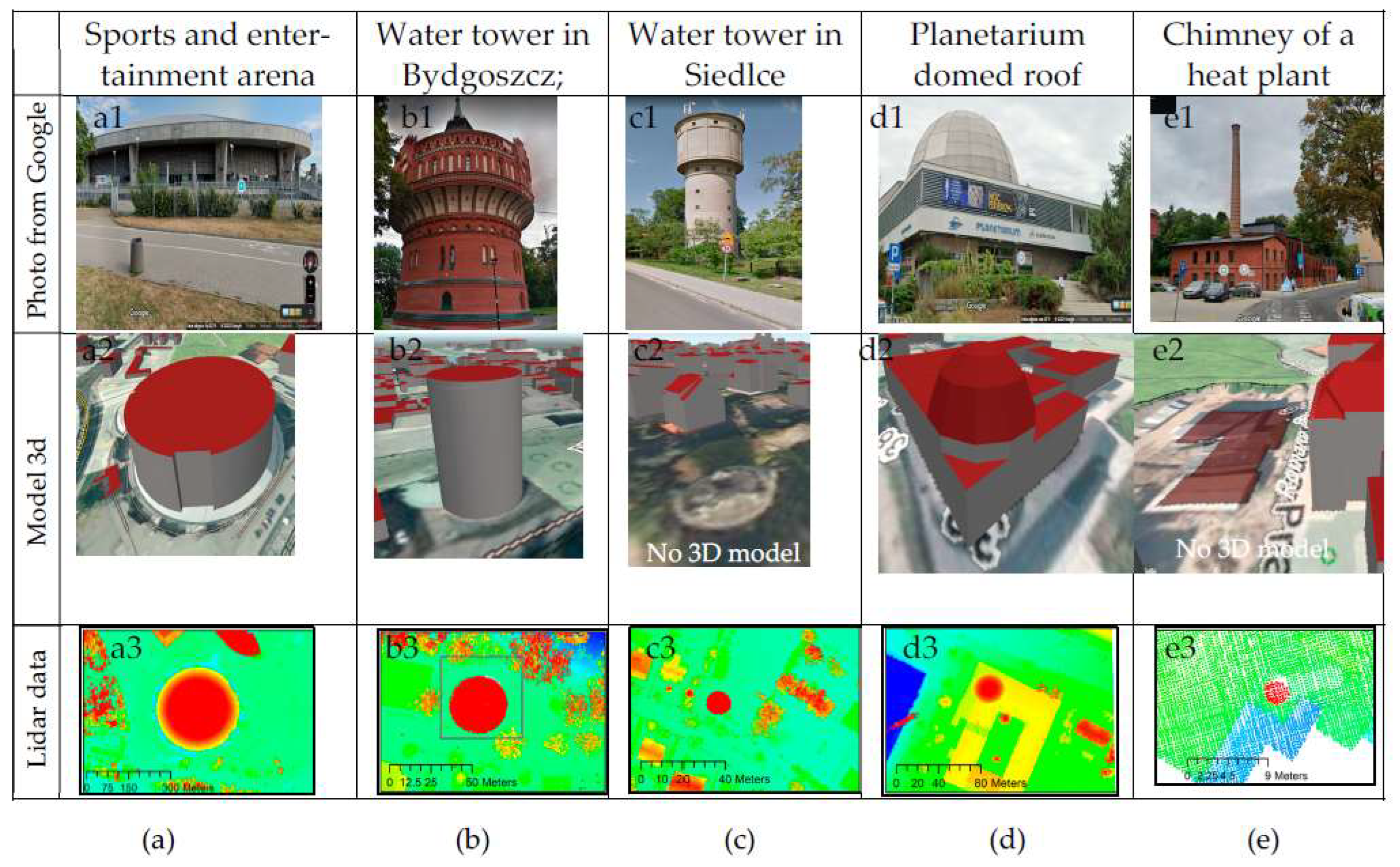
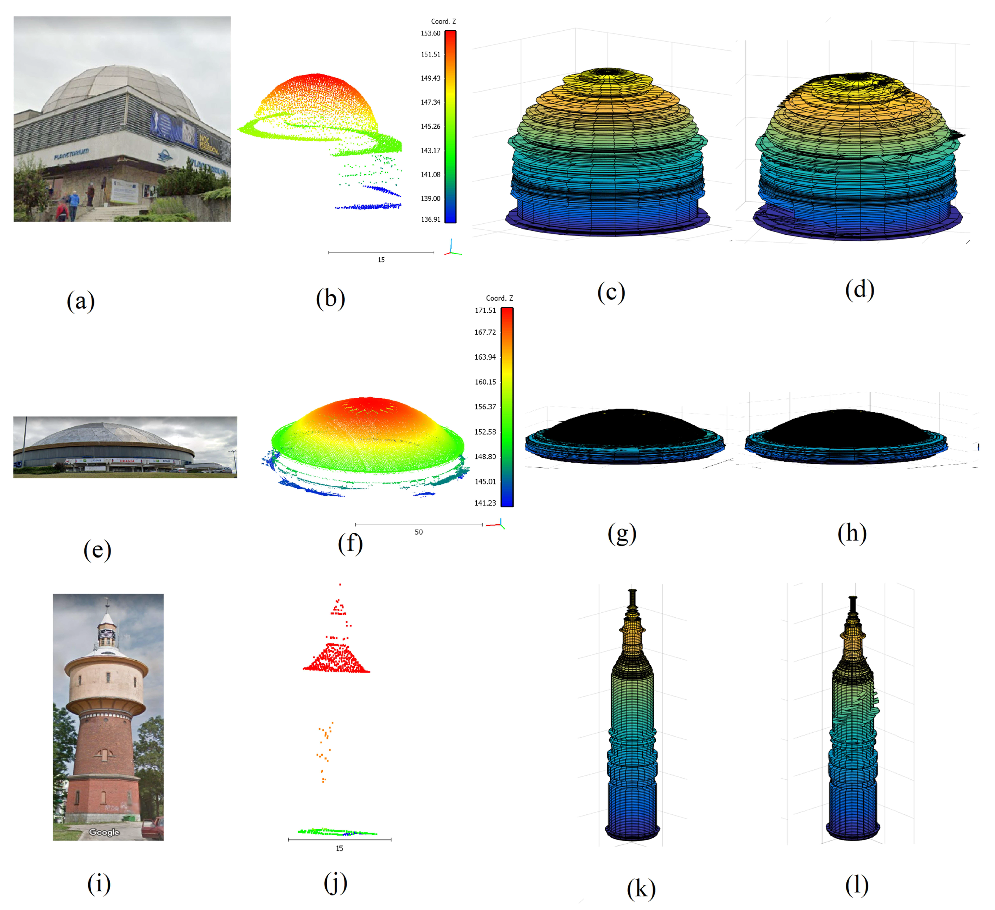
The presented study uses point clouds acquired with the airborne laser scanning (ALS) methods, representing distinctive buildings in the analyzed cities. These data were obtained from the Polish Spatial Data Infrastructure (SDI). Buildings with atypical shapes, features, and heights often constitute landmarks in urban spaces. They include sports and entertainment arenas, water towers, buildings with domed roofs (such as planetariums), or industrial buildings with tall chimneys (Figure 1).
These building models are largely simplified at the LoD2 level in the 3D models of Polish cities developed. They are represented by cylinders or are overlooked in models (Figure 1(a1,a2,b1,b2,c1,c2,d1,d2,e1,e2)). Points representing buildings that are rotational surfaces can be extracted from a LiDAR. When classifying points by height and viewing the vertical projections of the LiDAR sets, one can distinguish clusters of points showing the tested objects in the shape of circles (Figure 1). Selected for the study are different types of buildings (Figure 1a–c) and elements of building (Figure 1d,e).
Data files are acquired in LAZ format, while the point coordinates are expressed in the ETRS_1989_Poland_CS92 (EPSG 2180) coordinate system. All points are assigned class ID, signal intensity values, and RGB values from aerial images. The scanning was acquired in 2017–2022 with a resolution of 12 or 4 points per square meter, depending on the year of acquisition.
4. Method
Successive stages of the modeling process are described in the following subsections.
4.1. Improve Vertical Cross-Section Point Cloud
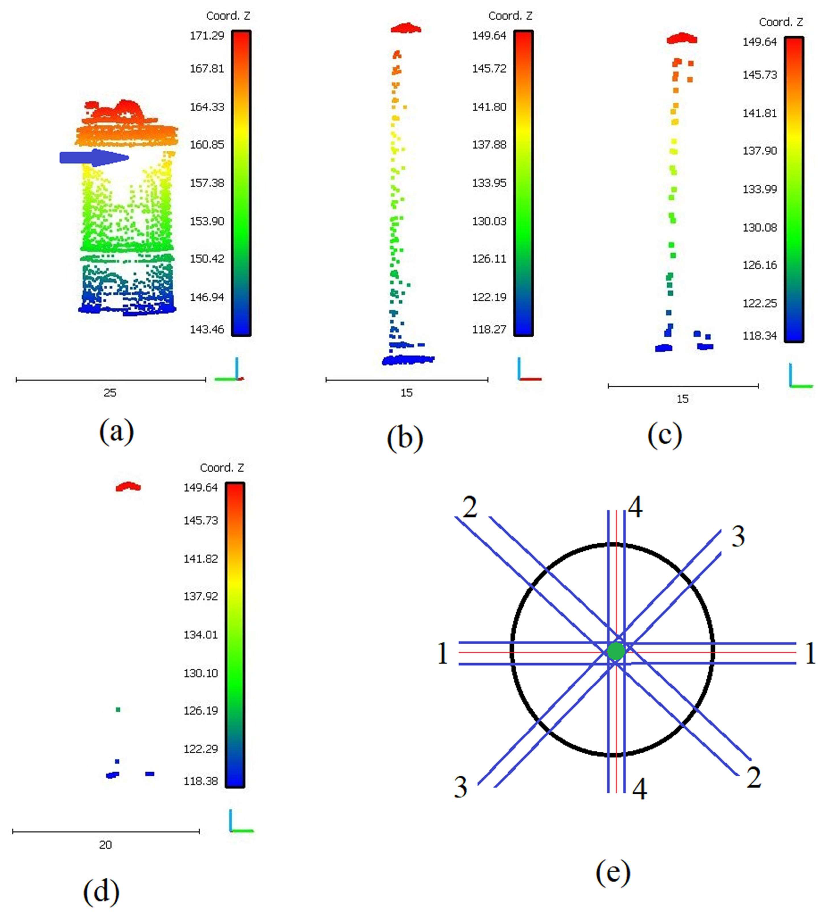
From Figure 2a,b, it can be noted that the point density, as well as the point distribution on the vertical walls of a tower point cloud, are heterogeneous. As an example, the calculation of two vertical cross-sections of the point cloud illustrated in Figure 2b according to two different directions (direction 1-1 and direction 4-4, as shown in Figure 2e) provides two different results shown in Figure 2c,d. In fact, the difference between the two obtained results is due to the irregular distribution of LiDAR points on the building facades. At this stage, the major question that arises is in which direction (according to Figure 2e) the vertical cross-section must be calculated to obtain the best representative result. This paper proposes a new approach to calculate the best cross-section that considers all LiDAR points describing the tower building.
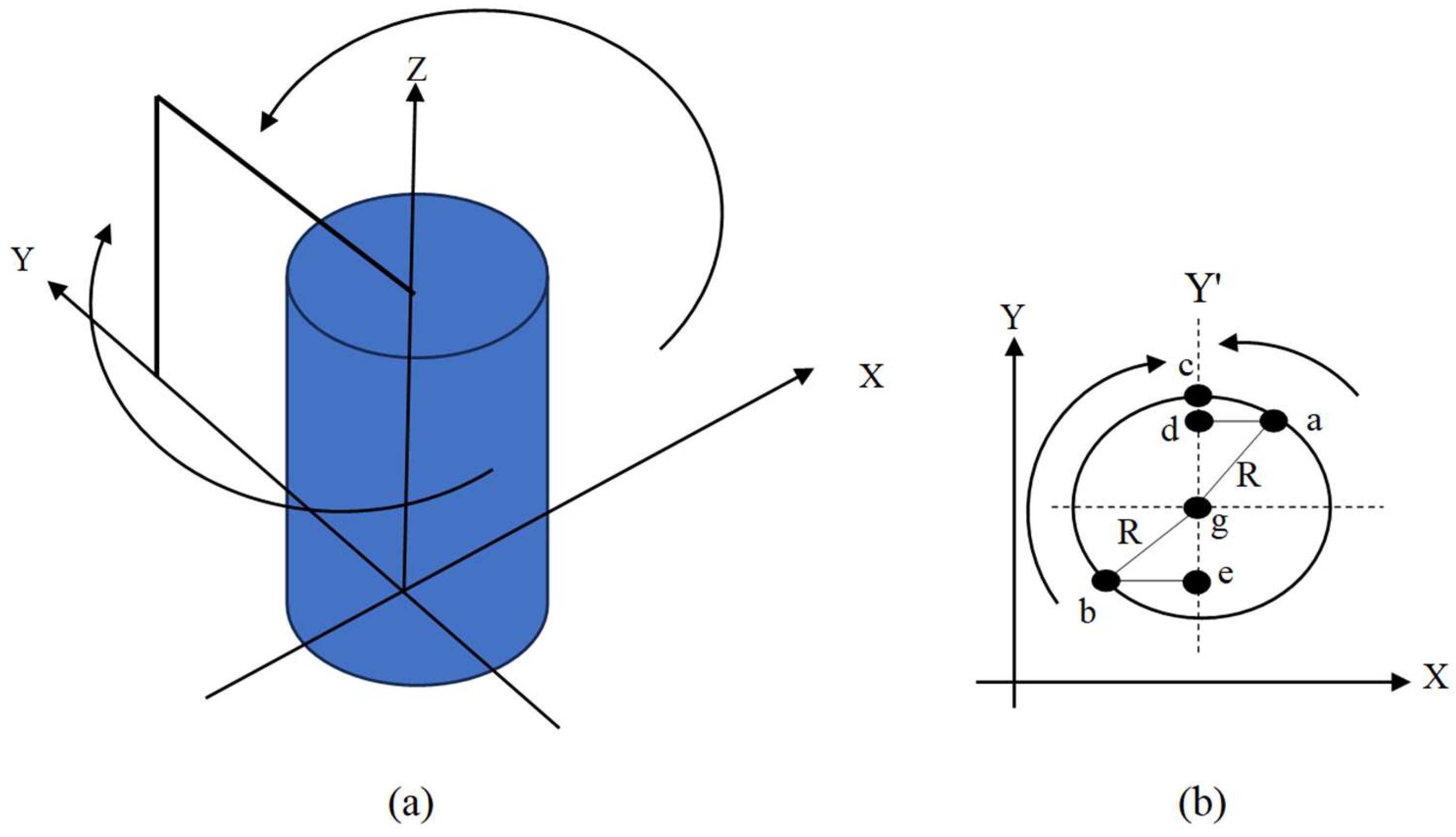
The first step is to project all points according to a circular trajectory and then group them into one half vertical plane located on one side of the tower (Figure 3). To carry out this operation, the cloud coordinates (X, Y, and Z) are transformed into a plane coordinate system (X1 and Y1) according to Equation (1).
where Xg and Yg are the coordinates of the point cloud gravity center according to Lewandowicz et al. [45] as shown in Equation (2).
To clarify this operation, the example illustrated in Figure 3b is detailed. In Figure 3b, the distances are equal between all points of the circle and the gravity center (the circle center) and equal to R (the circle radius). Point ‘a’ is projected in a circular trajectory on the same circle, the obtained result is Point ‘c’. The same operation is applied to Point ‘b’, and the obtained result will also be Point ‘c’. In Equation (1), as Points ‘a’ and ‘b’ have the same Z value and their distances to the gravity center are the same, the new coordinate X1 of the two points will be the same. At this stage, it is important to refer that this operation does not represent a projection on gY’ axis. Indeed, the projection of Points ‘a’ and ‘b’ on axis gY’ are consecutively Points ‘d’ and ‘e’.
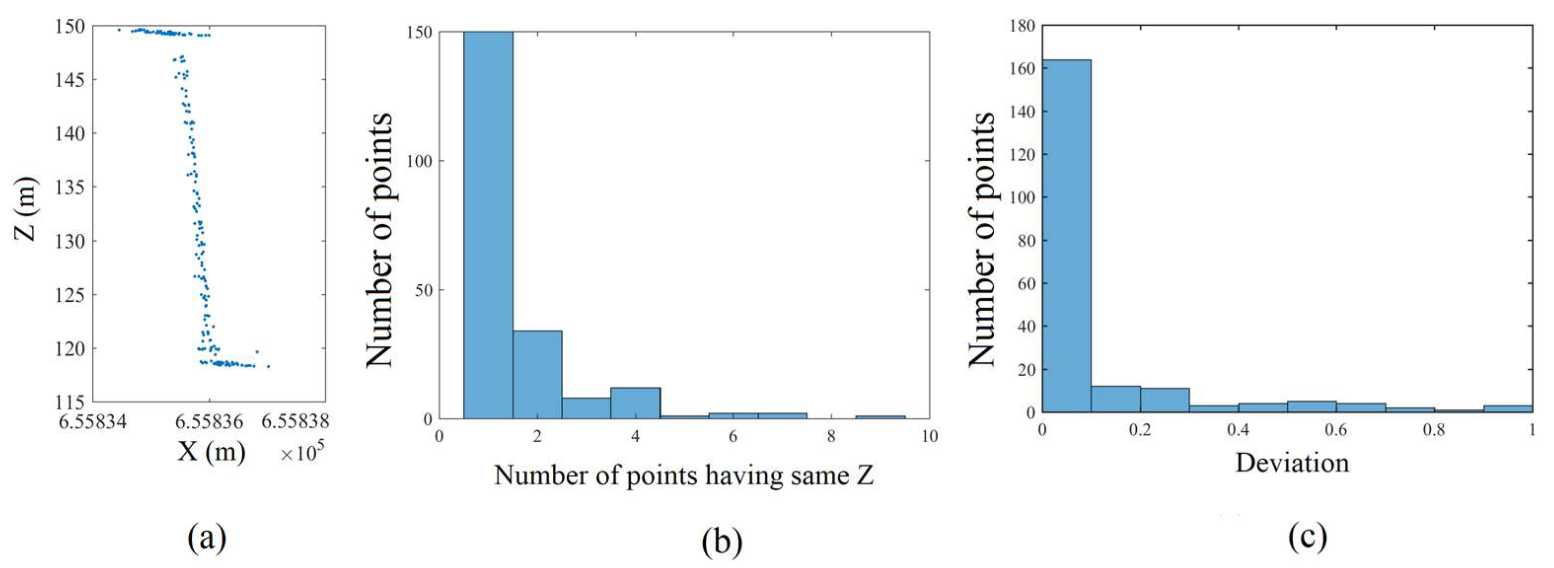
Thereafter, the new point cloud {X1, Y1} which represents the vertical cross-section, should be put in descending order regarding the Z coordinate values. At this stage, it can be noted that according to the point density, it is possible to present groups of points having the same Z coordinate value. In fact, there are three considerations to present this kind of point: LiDAR point accuracy, texture smoothing, and building architecture. The basic hypothesis in the suggested approach is that one building surface consists of a main rotating surface and some decoration parts added to this surface. Hence, in the case of several points having the same Z values and different distances from the rotating axis, the nearest point to the rotating axis is located on the main rotating surface, whereas further points are likely located on the decorations. If the building architecture reason is neglected, then the basic frustum of a cone must pass through the central point. Moreover, if the point accuracy and texture smoothing are neglected, then the basic frustum of a cone must pass through the nearest point to the rotating axis. Furthermore, if it is desired to consider all of the three reasons together, the points of the same Z coordinate value must be divided into two groups: one group of points that belong to the main building surface and the other that belongs to the decoration. This analysis needs more experiments to decide if it is efficient or not. Finally, as all available points will be considered in the model equation, the errors will only be located at places where points are missing.
In this paper, a new rule is added, as follows: if a group of points has the same Z coordinate value, only the farthest point from the rotation axis is kept; the other points are temporarily eliminated until the last modeling step.
This procedure allows for a reduction of the number of points of the vertical cross-section. The new cross-section point cloud is noted as a reduced point cloud. In this context, a new list that has the same length as the reduced point cloud is defined and named the point-frequency list. This list represents, for each point of the reduced point cloud, the number of points having the same Z coordinate value in the original point cloud. Another list named dev_list is defined. For the points having point-frequency values greater than one, the value of the corresponding dev-list cell is equal to the subtraction of the nearest and farthest distances from the rotating axis. If the point-frequency value is equal to one, in this case, the corresponding dev-list cell is assigned zero.
Figure 4a visualizes the reduced vertical cross-section of the tower point cloud shown in Figure 2b. Figure 4b uses the histogram illustration to visualize the frequent list of point clouds shown in Figure 4. In this figure, it can be noted that the frequency of the most reduced point clouds is equal to one. The maximum value of the frequency is equal to 10. In fact, the importance of this list as well as the dev_list will be highlighted in the third improvement step. Figure 4c utilizes histogram graphics to visualize the dev_list of the point cloud shown in Figure 4a. In this figure, it can be stated that most reduced cross-section points do not have deviations from the building model. Moreover, points with deviations can be classified into two classes. The first class is the points with small and neglected deviations comparable to the LiDAR point accuracy of 0.4 m or smaller. The second class is the points having a deviation greater than 0.4 m due to the presence of decoration or noise.
4.2. Gap Analysis and Filling
Once the cross-section point cloud is calculated and reduced, the next step is the vertical cross-section gaps analysis. The mean expected distance between two neighboring points depends on the point density. In the building point cloud, it is common to meet neighboring points separated by distances greater than the mean expected distances; this separation distance is named a gap. However, two kinds of such gaps can be distinguished: horizontal gaps when the greater separation distance is horizontal (see blue arrow in Figure 2a), and vertical gaps when the greater separation distance is vertical. In fact, there are several reasons for the presence of these gaps, such as the obstacles that prevent the laser pulses to arrive at the scanned surface, the geometric form of the reflecting object, the physical nature of the scanned surface (e.g., the surface is made of glass), and the scanning parameters such as the flying height and the building location regarding the sensor location. Though the employment of the vertical cross-section to model the building can cancel the direct influence of the horizontal gaps because it moves all building points through a circular trajectory to group them into a vertical plane. But in the final obtained model, the presence of the horizontal gaps may reduce the building model accuracy in the gap zone due to the lack of information in this area. Concerning the vertical gaps, despite their influence being reduced through using the vertical cross-section described in the last section, sometimes these gaps still appear in the vertical cross-section (Figure 5) because all cloud points are grouped into one vertical plane (Figure 3). Therefore, it is necessary to add a special procedure to process the remaining vertical gaps and reduce the depicted deformation due to these kinds of gaps.
When a line segment is revolved around an axis, it mathematically draws a piece of a cone called the frustum of a cone. This frustum of a cone could be a cylinder when the line segment is parallel to the rotating axis. According to this principle and in the case of vertical gaps (Figure 5a,b), if the upper and the lowest gap points have different distances from the rotating axis (Figure 5b,c), the gap will generate a frustum of a cone connecting the two consecutive frusta of cones or cylinders in the building model (Figure 6b). In fact, this solution does not consider the main reason for the gap presence when the geometric form of the scanned surface prevents the laser pulses to arrive at the scanned object. That is why there is a great deformation in the gap area in the building model presented in Figure 6b. Hence, to improve the calculated building model, this paper proposes a new strategy to fill the gaps in the vertical cross-section as follows.
In the last section, the reduced point cloud was put in descending order regarding the Z coordinate values, which means that the first point in the list has the greater Z value and the last point in the list has the lowest Z value. At this stage, a new list, named Zspacing, is defined. The first cell in this list contains the value zero. Thereafter, the value of each cell is calculated by subtracting the Z coordinates value of the corresponding point in the reduced point cloud from its precedent point.
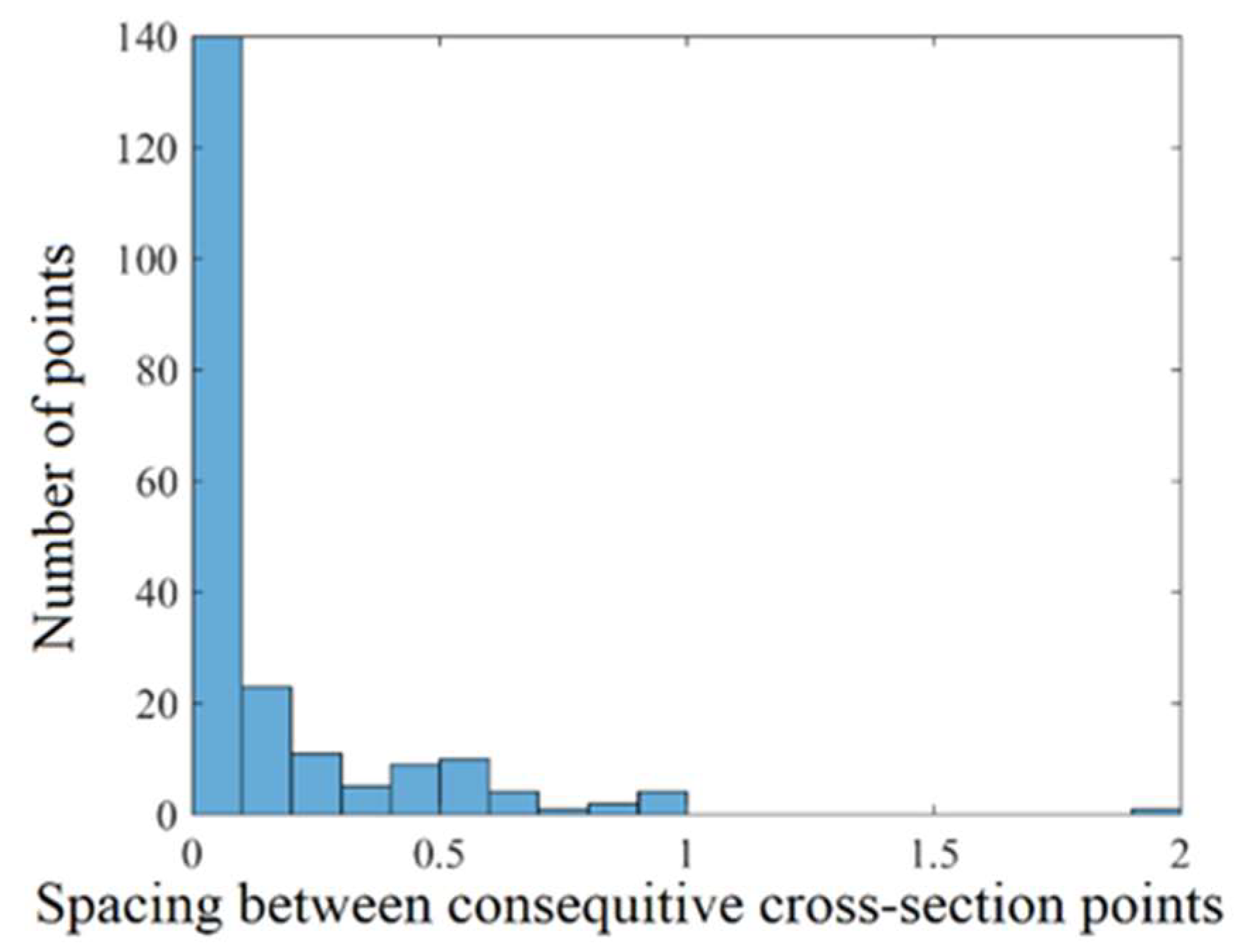
Figure 7 illustrates the visualization of the distribution of Zspacing cell values. In this histogram, it can be noted that the vertical spacing between most of the reduced cross-section cloud points is around zero. Moreover, the points having vertical spacing smaller than a given threshold (e.g., 0.2 m) can be considered as points having accepted vertical spacing and then having no gaps. Also, points having vertical spacing greater than the same threshold are considered points having gaps. In fact, the employed threshold value (THspacing = 0.2 m) depends on the point density. Its value can be considered equal to or smaller than the mean expected distance between two neighboring points.
Once the Zspacing list is calculated and the spacing threshold is determined, the point gaps can be detected by comparing the vertical space values with the spacing threshold. To fill a gap, a list of points is added within the gap. These points have the same abscissa of the gap’s lowest point (Figure 5c) and have gradual ordinates starting from the gap’s lowest point ordinate added to THspacing until the gap’s upper point ordinate.
Figure 6 and Figure 8 show the modeling results of the building point clouds illustrated in Figure 2b and Figure 5a consecutively in the case of the application of the gap-filling strategy and without applying this strategy. In Figure 8, the gap heights are smaller than those in Figure 6, which is why the influence of the filling gap operation is less notable oppositely to the case of the building presented in Figure 6. In Figure 6b, the building model has a great deformation in the gap area. This deformation disappears in Figure 6c thanks to the gap-filling function. Moreover, the building model becomes more faithful to the original building presented in Figure 6a after applying the gap-filling strategy.
4.3. Integrating Deviated Points in the Calculated Model
It can be observed from Figure 4b that most of the building cloud points have distinctive (non-duplicated) Z coordinate values. However, in the presence of several LiDAR points having the same Z coordinate value, the suggested algorithm in the last section considers only the nearest point to the rotating axis and neglects the other points. In this section, the suggested algorithm will be extended to consider all cloud points without neglect. For this purpose, the coordinates of non-considered points are used to modify the rotating surface depicted by Equations (3)–(5) [45].
At this stage, it is important to show how Equations (3)–(5) are deduced. One rotating surface can be divided into n horizontal slices according to the consecutive Z coordinate values of the half -cross-section cloud (see Figure 4a). The points of each slice have the same Zi coordinate value, which is why the elements of each row in the Z matrix are equal. Each slice represents a circle because it belongs to a rotating surface. This circle can be divided into m angular sectors. One rotating surface is expressed by three matrices X, Y, and Z. This surface is composed of cells. The coordinates of the middle point of each cell will be considered from the three corresponding cells of the last three matrices. The dimensions of one cell can be calculated as a function of the thickness of the horizontal slice, the number of angular sectors, and the cell circle radius value (R = Yi − Yg). The angle of each angular sector equals , where j is the sector number. In Equation (5), the origin of β is the circle center, but the origin of α is Yi. The application of basic sine and cosine relationships allows deducing α and β equations where the value is added to the angle value for adapting the signs.
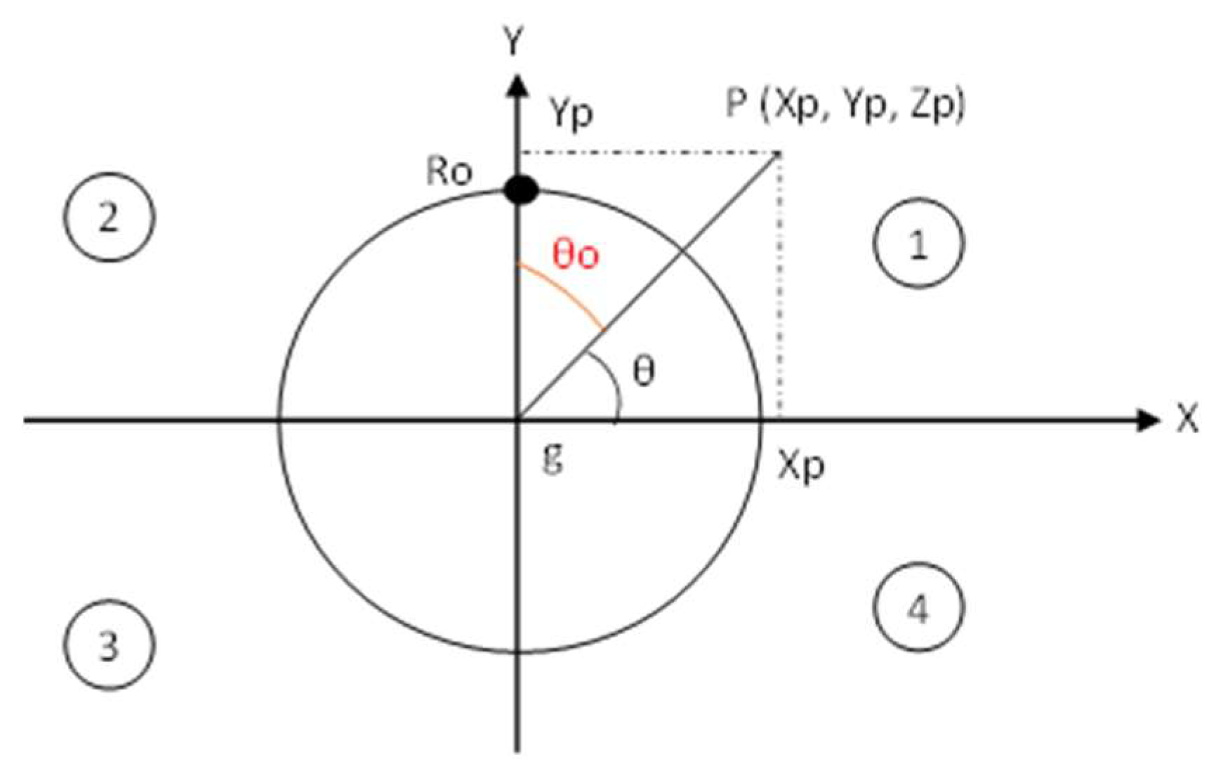
Return to the integration of non-considered points, if one point (Xp, Yp, Zp) does not belong to a rotating surface defined by Equations (3)–(5), it is desired to integrate this point within this surface. Hence, this operation can be carried out by calculating the angle θ (see Figure 9) using Equation (6). Thereafter, the angle θo measured from the rotating origin Ro (see Figure 9) is calculated according to Equation (7). In the matrices X and Y, the row number of the concerned cell can be calculated depending on the Z coordinate value (Zp). Furthermore, the column number of the concerned cell can be calculated depending on θo value and the number of columns of the matrix X according to Equation (3).
where Xg and Yg are the coordinates of the gravity center (Equation (2)); Xi, Yi, and Zi (i = 1 to n) are the point coordinates of the half cross-section; j = 1 to m; n is the number of points in the half cross-section; and βi are the step values of X and Y, respectively; and m is the number of columns in matrix X.
where CN is the column number in matrix X (Equation (3)), m is the number of columns in matrix X, and “round” is a function that provides the round value of a given real number.
The new value of the corresponding cells in X and Y matrices are calculated using Equation (9).
where Xn and Yn are the new value of the corresponding cells in X and Y matrices, Dispg is the distance between the gravity center g and the given point P.
Once the new value of the corresponding cells in the X and Y matrices are calculated, these values can be reassigned to the concerned cell in the matrices X and Y. This operation can be carried out for all deviated points to consider them within the building model.
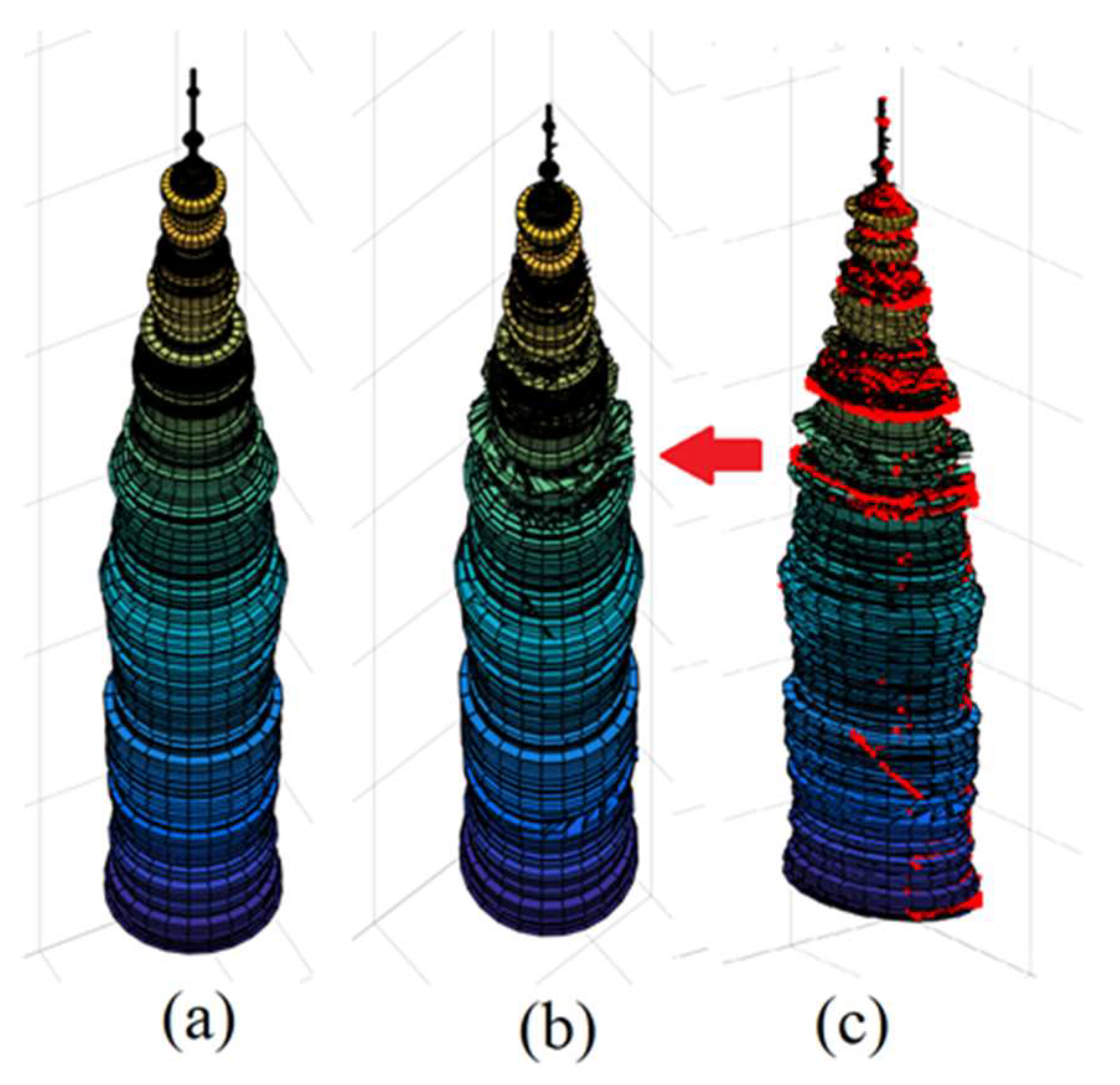
The red arrow in Figure 8c points to the influence due to the integration of the deviated points within the building model. Unfortunately, the deviated points in the case of the building illustrated in Figure 8 represent noisy points, which is why the constructed model shown in Figure 8c has certain deformations due to the inclusion of noise points. However, the inclusion of the deviated points may sometimes improve the model quality when the deviated point density is high enough, and the deviated points represent building details or decoration. Figure 10a,b show the tower model before and after the inclusion of the deviated points. At the red arrow in Figure 10c, the geometry of the tower part covered by the LiDAR points (see Figure 10c, which shows the superimposition of the point cloud on the building model) was improved due to considering all LiDAR points. Moreover, Figure 10c illustrates that the tower point cloud completely fits the improved constructed model. Nevertheless, more investigations are needed to automatically classify the building point cloud into building points and noise points.
5. Discussion
In this section, the suggested modeling algorithm will be applied to different samples of the tower point clouds. Then, the modeling accuracy as well as the faithfulness of the obtained models will be discussed.
5.1. Performance of the Method
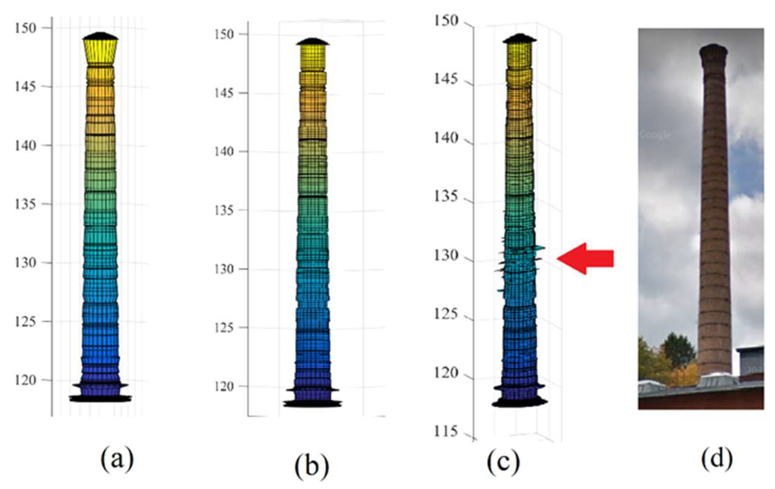
Figure 6, Figure 8, Figure 10, Figure 11 and Figure 12 depict the tower models constructed by the proposed approach. Figure 6 and Figure 8 show the influence of gap-filling operation on the constructed building model, where this influence is humble in the case of the building illustrated in Figure 8 because the geometric form of the tower does not contain a hidden area regarding the airborne scanning, whereas in the case of building illustrated in Figure 6, the gap filling operation is crucial in order to avoid the huge deformation within the hidden area. Nevertheless, the success of the gap-filling procedure needs sufficient points to cover the tower body. This situation can be illustrated in Figure 11i–l. The LiDAR points that cover the building body are concentrated only on the upper part of the tower, in contrast to the other lower parts, where very few points are laid on the building body’s outer surfaces. That is why the obtained building model cannot show the steps of building architectural form (Figure 11k,l). In the same context, the gap-filling procedure depends on the vertical spacing threshold value, which is related to the point density as well as the LiDAR point accuracy.
Moreover, in the building vertical cross-section, the accepted vertical spacing value between neighboring points is variable regarding the regularity level of point distribution, point accuracy, point density, building architectural form and complexity level, construction material nature, and scanning angle. More investigation is needed to improve the selection and effect of the vertical spacing between neighboring points.
Concerning the integration of deviated points operation, two cases may be envisaged. First, when the deviated points represent noisy points, the integration of these points within the building calculated model will produce undesired deformations (see red arrow in Figure 8c). Second, if the deviated points do not represent noisy points, the integration of these points into the constructed building model may improve its quality if their density value is elevated enough because it will become more faithful to the scanned building (Figure 10b,c, Figure 11, and Figure 12). On the other hand, if the deviated points’ density is low, the introduced corrections may make the building model look deformed. Furthermore, the resemblance level between the obtained building model and the original scanned building will be related to the point density and accuracy values. At this stage, more investigations in future research are requested about the effective integration of the deviated points into the constructed tower model.
Though the high efficiency of the suggested approach is demonstrated regarding the architectural complexity of the target buildings, it still suffers from some limitations that deserve future efforts. These limitations can be summarized as follows:
- Undesirable distortions may appear in the constructed model when the input point cloud has inconsistent quality regarding the point density, distribution regularity, and homogeneity. Certain levels of balance may be desired that can comprise the data volume, level of details for presentation, and the accuracy of the model;
- Like many other methods, the developed method can only reconstruct buildings that meet certain assumptions, which in this case are rotating surfaces. Small attachments or decorations of the main surface need to be treated separately. A promising effort is to extend and/or integrate this method with other methods to handle complex and diverse buildings.
5.2. Modeling Accuracy
Concerning the accuracy of the constructed building models, there are two main accuracy estimating approach families [22]. First, the created building model is compared with the reference model constructed manually or semi-automatically using LiDAR data or other data sources such as aerial images [14,20,21]. In the second approach, the LiDAR point cloud is employed as a reference model, where the accuracy can be evaluated by calculating the distances between the constructed building model and the point cloud [20,21,28]. In this paper, the accuracy of modeling will be discussed through three viewpoints. First, despite the undesirable deformations in the constructed building models, the accuracy of the calculated building model is 100% when the building point cloud is considered as a reference model. Indeed, the constructed model fits all building cloud points and, consequently, the building model is completely faithful to the input building point cloud. In this context, Tarsha Kurdi and Awrangjeb [22] compared the building point clouds with the obtained building models. They concluded that the accuracy, regularity, as well as point density of the building point cloud, may affect the faithfulness of the building model to the original building even if the model greatly fits the point cloud.
From a second viewpoint, the cell’s dimension of the model can also express the building model accuracy, because the cell size represents the interval where the LiDAR point may be located. From Equations (3)–(5), the building model consists of a matrix of cells connected through robust neighbor relationships. The cell’s dimensions are used as an evaluation metric. The width (CW) and height (CH) of a cell can be calculated using Equation (10).
where is the distance between the gravity center g and the given point (Equation (11)), is the number of columns in matrix X.
From Equation (10), it can be noted that the cell’s dimensions are related to the number of columns in the building model matrices, the distance from the rotating axis, and the point density. While the number of columns of the model matrices increases, the cell widths will decrease. Also, CW and CH values are variable from point to point in the building model. Hence, for each building model, the minimum, maximum, and mean values of these parameters are calculated (Table 1). In this context, the buildings illustrated in Figure 11 and Figure 12 are considered to estimate the modeling accuracy by respecting their order.
From Table 1, it can be noted that at least one dimension of the cell is related to the building diameter. That is why it is advised to increase the m value with an increase in the building radius. To conclude, two main factors that influence the dimension of the model cells are the building diameter and the point density.
Finally, in the same context of the building model accuracy, the question of accuracy estimation by comparing the constructed building model with a reference model constructed manually or semi-automatically [14,20,21] will also be discussed. In fact, the target buildings by the proposed modeling approach have complicated architectural forms (see Figure 6, Figure 8, Figure 10, Figure 11 and Figure 12), where their geometric forms contain curved surfaces as well as decorations. That is why the construction of accurate models for them to be used as references will need a huge amount of time and extra data and measurements. Moreover, if it is insisted to construct these reference models, a new question will arise concerning the comparison between the reference model and the calculated models. Indeed, the references model is supposed to have vectorial forms, whereas one calculated building model is composed of three matrices (X, Y, and Z). Also, the visualization of the calculated models is carried out using 3D pixel form because the model represents a novel modeling strategy in the world of LiDAR data and is based on the concept of the rotating surface. Hence, the comparison between the two building models needs more investigation.
To conclude, in this paper, only the comparison between the calculated building model and its LiDAR point cloud is considered. In future research, a more thorough investigation will be carried out to compare the constructed models with the reference models. Another question about the improvement of quality as well as the accuracy of the calculated building model will also be handled.
6. Conclusions
The novel proposed approach to modeling atypical landmark buildings at the LoD3 level has significant implications for all applications that rely on 3D building models. The suggested algorithm is based on the hypothesis of the rotating surface form of the target building. One building point cloud will be present by three matrices, X, Y, and Z. Moreover, the visualization will be realized using 3D pixel form. Only buildings that are solids of the revolution were modeled in the present study. A strategy for filling gaps in vertical cross-sections was described for buildings whose unique features prevent laser pulses from reaching the scanned surface. The developed strategy significantly improved the quality of the generated models. The operation of integration of the deviated points into the constructed building model aids in completely fitting the constructed model with the point cloud, but it may generate undesirable deformation in the building model when the deviated points represent noisy points, or their density is not great enough.
The main advantage of the suggested modeling algorithm is that it targets complicated geometric buildings, and the model data volume is light. Further efforts are needed to render building facades in greater detail because the deviated points (outliers) in the calculated models can belong to the façade. These points can result from noise, residual errors in the process of determining the building axis, or even permissible deviations from the wall and roof surfaces stipulated in structural designs. Also, more investigations are needed to estimate the constructed building model with vectorial models.
Finally, the novel suggested modeling strategy can be extended in future work to be employed for most levels of building architectural complexity, especially when a high point density is available. This approach can be extended for tree modeling as well as statues and other solid objects.
Author Contributions
Conceptualization, F.T.K., E.L. and Z.G.; methodology, F.T.K. and E.L.; software, F.T.K.; validation, F.T.K. and J.S.; formal analysis, F.T.K. and J.S.; resources, E.L., data curation, F.T.K. and E.L.; writing—original draft preparation, F.T.K. writing—review and editing, Z.G. and J.S.; visualization, F.T.K., E.L. and J.S. All authors have read and agreed to the published version of the manuscript.
Funding
This research was financed as part of a statutory research project of the Faculty of Geoengi neering of the University of Warmia and Mazury in Olsztyn, Poland, entitled “Geoinformation from the Theoretical, Analytical and Practical perspective” (No. 29.610.008-110_timeline: 2023–2025).
Data Availability Statement
The publication uses LAS measurement data obtained from an open Polish portal run by the Central Office of Geodesy and Cartography, and street view images were used. Water towers were searched based on the portal https://wiezecisnien.eu/en/wieze-cisnien/, accessed on 25 June 2023.
Acknowledgments
We would like to thank the Central Office of Geodesy and Cartography (GUGiK) in Poland for providing Lidar measurement data and for making data from the 3D portal available.
Conflicts of Interest
The authors declare no conflict of interest.
References
- Richa, J.P.; Deschaud, J.-E.; Goulette, F.; Dalmasso, N. AdaSplats: Adaptive Splatting of Point Clouds for Accurate 3D Modeling and Real-Time High-Fidelity LiDAR Simulation. Remote Sens. 2022, 14, 6262. [Google Scholar] [CrossRef]
- Beil, C.; Ruhdorfer, R.; Coduro, T.; Kolbe, T.H. Detailed Streetspace Modelling for Multiple Applications: Discussions on the Proposed CityGML 3.0 Transportation Model. ISPRS Int. J. Geo-Inf. 2020, 9, 603. [Google Scholar] [CrossRef]
- Biljecki, F.; Lim, J.; Crawford, J.; Moraru, D.; Tauscher, H.; Konde, A.; Adouane, K.; Lawrence, S.; Janssen, P.; Stouffs, R. Extending CityGML for IFC-sourced 3D city models. Autom. Constr. 2021, 121, 103440. [Google Scholar] [CrossRef]
- Jayaraj, P.; Ramiya, A.M. 3D CityGML building modelling from lidar point cloud data. In The International Archives of Photogrammetry, Remote Sensing and Spatial Information Sciences; Gottingen Tom XLII-5; Copernicus GmbH: Gottingen, Germany, 2018; pp. 175–180. [Google Scholar] [CrossRef] [Green Version]
- Xu, Y.; Stilla, U. Towards Building and Civil Infrastructure Reconstruction From Point Clouds: A Review on Data and Key Techniques. IEEE J. Sel. Top. Appl. Earth Obs. Remote Sens. 2021, 14, 2857–2885. [Google Scholar] [CrossRef]
- Tarsha Kurdi, F.; Awrangjeb, M.; Liew, A.W.-C. Automated Building Footprint and 3D Building Model Generation from Lidar Point Cloud Data. In Proceedings of the 2019 Digital Image Computing: Techniques and Applications (DICTA), Perth, Australia, 2–4 December 2019; pp. 1–8. [Google Scholar] [CrossRef]
- Tarsha Kurdi, F.; Gharineiat, Z.; Campbell, G.; Dey, E.K.; Awrangjeb, M. Full Series Algorithm of Automatic Building Extraction and Modelling from LiDAR Data. In Proceedings of the 2021 Digital Image Computing: Techniques and Applications (DICTA), Gold Coast, Australia, 29 November–1 December 2021; pp. 1–8. [Google Scholar] [CrossRef]
- Labetski, A.; Vitalis, S.; Biljecki, F.; Ohori, K.A.; Stoter, J. 3D building metrics for urban morphology. Int. J. Geogr. Inf. Sci. 2023, 37, 36–67. [Google Scholar] [CrossRef]
- Pfeifer, N.; Rutzinger, M.; Rottensteiner, F.; Muecke, W.; Hollaus, M. Extraction of Building Footprints from Airborne Laser Scanning: Comparison and Validation Techniques. In Proceedings of the Joint IEEE-GRSS/ISPRS Workshop on Remote Sensing and Data Fusion over Urban Areas, Urban 2007, Paris, France, 11–13 April 2007. [Google Scholar] [CrossRef]
- Wang, X.; Luo, Y.-P.; Jiang, T.; Gong, H.; Luo, S.; Zhang, X.-W. A New Classification Method for LIDAR Data Based on Unbalanced Support Vector Machine. In Proceedings of the 2011 International Symposium on Image and Data Fusion, Tengchong, China, 9–11 August 2011; pp. 1–4. [Google Scholar] [CrossRef]
- Chen, D.; Zhang, L.; Mathiopoulos, P.; Huang, X. A Methodology for Automated Segmentation and Reconstruction of Urban 3-D Buildings from ALS Point Clouds. IEEE J. Sel. Top. Appl. Earth Obs. Remote Sens. 2014, 7, 4199–4217. [Google Scholar] [CrossRef]
- Sampath, A.; Shan, J. Building Boundary Tracing and Regularization from Airborne Lidar Point Clouds. Photogramm. Eng. Remote Sens. 2007, 73, 805–812. [Google Scholar] [CrossRef] [Green Version]
- Gilani, S.A.N.; Awrangjeb, M.; Lu, G. Segmentation of Airborne Point Cloud Data for Automatic Building Roof Extraction. GIScience Remote Sens. 2017, 55, 63–89. [Google Scholar] [CrossRef] [Green Version]
- Jung, J.; Sohn, G. Progressive modeling of 3D building rooftops from airborne Lidar and imagery. In Topographic Laser Ranging and Scanning: Principles and Processing, 2nd ed.; Shan, J., Toth, C.K., Eds.; Taylor & Francis Group; CRC Press: Boca Raton, FL, USA, 2018; pp. 523–562. Available online: https://www.taylorfrancis.com/chapters/edit/10.1201/9781315154381-17/progressive-modeling-3d-building-rooftops-airborne-lidar-imagery-jaewook-jung-gunho-sohn (accessed on 25 June 2023).
- Dey, E.K.; Tarsha Kurdi, F.; Awrangjeb, M.; Stantic, B. Effective Selection of Variable Point Neighbourhood for Feature Point Extraction from Aerial Building Point Cloud Data. Remote Sens. 2021, 13, 1520. [Google Scholar] [CrossRef]
- Dong, Y.; Hou, M.; Xu, B.; Li, Y.; Ji, Y. Ming and Qing Dynasty Official-Style Architecture Roof Types Classification Based on the 3D Point Cloud. ISPRS Int. J. Geo-Inf. 2021, 10, 650. [Google Scholar] [CrossRef]
- Tarsha Kurdi, F.; Awrangjeb, M.; Munir, N. Automatic filtering and 2D modeling of LiDAR building point cloud. Trans. GIS 2020, 25, 164–188. [Google Scholar] [CrossRef]
- Mahphood, A.; Arefi, H. Density-based method for building detection from LiDAR point cloud. ISPRS Ann. Photogramm. Remote Sens. Spatial Inf. Sci. 2023, X-4/W1-2022, 423–428. [Google Scholar] [CrossRef]
- Park, S.-Y.; Lee, D.G.; Yoo, E.J.; Lee, D.-C. Segmentation of Lidar Data Using Multilevel Cube Code. J. Sens. 2019, 2019, 4098413. [Google Scholar] [CrossRef]
- Cheng, L.; Zhang, W.; Zhong, L.; Du, P.; Li, M. Framework for Evaluating Visual and Geometric Quality of Three-Dimensional Models. IEEE J. Sel. Top. Appl. Earth Obs. Remote Sens. 2014, 8, 1281–1294. [Google Scholar] [CrossRef]
- Ostrowski, W.; Pilarska, M.; Charyton, J.; Bakuła, K. Analysis of 3D building models accuracy based on the airborne laser scanning point clouds. In International Archives of the Photogrammetry, Remote Sensing & Spatial Information Sciences; ISPRS: Vienna, Austria, 2018; p. 42. Available online: https://ui.adsabs.harvard.edu/link_gateway/2018ISPAr.422..797O/ (accessed on 25 June 2023). [CrossRef] [Green Version]
- Tarsha Kurdi, F.; Awrangjeb, M. Comparison of LiDAR Building Point Cloud with Reference Model for Deep Comprehension of Cloud Structure. Can. J. Remote Sens. 2020, 46, 603–621. [Google Scholar] [CrossRef]
- Tarsha Kurdi, F.; Gharineiat, Z.; Campbell, G.; Awrangjeb, M.; Dey, E.K. Automatic Filtering of Lidar Building Point Cloud in Case of Trees Associated to Building Roof. Remote Sens. 2022, 14, 430. [Google Scholar] [CrossRef]
- Gharineiat, Z.; Tarsha Kurdi, F.; Campbell, G. Review of Automatic Processing of Topography and Surface Feature Identification LiDAR Data Using Machine Learning Techniques. Remote Sens. 2022, 14, 4685. [Google Scholar] [CrossRef]
- Adeleke, A.K.; Smit, J.L. Building roof extraction as data for suitability analysis. Appl. Geomat. 2020, 12, 455–466. [Google Scholar] [CrossRef]
- Yang, W.; Liu, X.; Zhang, Y.; Wan, Y.; Ji, Z. Object-based building instance segmentation from airborne LiDAR point clouds. Int. J. Remote Sens. 2022, 43, 6783–6808. [Google Scholar] [CrossRef]
- Axel, C.; Van Aardt, J. Building damage assessment using airborne lidar. J. Appl. Remote Sens. 2017, 11, 046024. [Google Scholar] [CrossRef] [Green Version]
- Dorninger, P.; Pfeifer, N. A Comprehensive Automated 3D Approach for Building Extraction, Reconstruction, and Regularization from Airborne Laser Scanning Point Clouds. Sensors 2008, 8, 7323–7343. [Google Scholar] [CrossRef] [Green Version]
- Liu, X.; Zhang, Y.; Ling, X.; Wan, Y.; Liu, L.; Li, Q. TopoLAP: Topology Recovery for Building Reconstruction by Deducing the Relationships between Linear and Planar Primitives. Remote Sens. 2019, 11, 1372. [Google Scholar] [CrossRef] [Green Version]
- Li, Z.; Shan, J. RANSAC-based multi primitive building reconstruction from 3D point clouds. ISPRS J. Photogramm. Remote Sens. 2022, 185, 247–260. [Google Scholar] [CrossRef]
- Liu, X.; Zhu, X.; Zhang, Y.; Wang, S.; Jia, C. Generation of concise 3D building model from dense meshes by extracting and completing planar primitives. Photogramm. Rec. 2023, 38, 22–46. [Google Scholar] [CrossRef]
- Matikainen, L.; Hyyppä, J.; Hyyppä, H. Automatic detection of buildings from laser scanner data for map updating. In International Archives of the Photogrammetry and Remote Sensing, XXXIV, 3/W13; ISPRS: Dresden, Germany, 2003; Available online: https://www.isprs.org/proceedings/xxxiv/3-W13/papers/Matikainen_ALSDD2003.pdf (accessed on 25 June 2023).
- Vosselman, G.; Dijkman, S. 3D Building Model Reconstruction from Point Clouds and Ground Plans. In International Archives of the Photogrammetry and Remote Sensing, XXXIV, 3/W4; ISPRS: Annapolis, MA, USA, 2001; pp. 37–44. [Google Scholar]
- Wen, C.; Yang, L.; Li, X.; Peng, L.; Chi, T. Directionally constrained fully convolutional neural network for airborne LiDAR point cloud classification. ISPRS J. Photogramm. Remote Sens. 2020, 162, 50–62. [Google Scholar] [CrossRef] [Green Version]
- Maltezos, E.; Doulamis, A.; Doulamis, N.; Ioannidis, C. Building Extraction from LiDAR Data Applying Deep Convolutional Neural Networks. IEEE Geosci. Remote Sens. Lett. 2018, 16, 155–159. [Google Scholar] [CrossRef]
- Yuan, J. Learning Building Extraction in Aerial Scenes with Convolutional Networks. IEEE Trans. Pattern Anal. Mach. Intell. 2017, 40, 2793–2798. [Google Scholar] [CrossRef] [PubMed]
- Kuras, A.; Brell, M.; Rizzi, J.; Burud, I. Hyperspectral and Lidar Data Applied to the Urban Land Cover Machine Learning and Neural-Network-Based Classification: A Review. Remote Sens. 2021, 13, 3393. [Google Scholar] [CrossRef]
- Zhou, L.; Geng, J.; Jiang, W. Joint Classification of Hyperspectral and LiDAR Data Based on Position-Channel Cooperative Attention Network. Remote Sens. 2022, 14, 3247. [Google Scholar] [CrossRef]
- Pantoja-Rosero, B.; Achanta, R.; Kozinski, M.; Fua, P.; Perez-Cruz, F.; Beyer, K. Generating LOD3 building models from structure-from-motion and semantic segmentation. Autom. Constr. 2022, 141, 104430. [Google Scholar] [CrossRef]
- Fan, H.; Wang, Y.; Gong, J. Layout graph model for semantic façade reconstruction using laser point clouds. Geo. Spat. Inf. Sci. 2021, 24, 403–421. [Google Scholar] [CrossRef]
- Gui, S.; Qin, R. Automated LoD-2 model reconstruction from very-high-resolution satellite-derived digital surface model and orthophoto. ISPRS J. Photogramm. Remote Sens. 2021, 181, 1–19. [Google Scholar] [CrossRef]
- Peters, R.; Dukai, B.; Vitalis, S.; van Liempt, J.; Stoter, J. Automated 3D Reconstruction of LoD2 and LoD1 Models for All 10 Million Buildings of the Netherlands. Photogramm. Eng. Remote Sens. 2022, 88, 165–170. [Google Scholar] [CrossRef]
- Zhang, Z.; Qian, Z.; Zhong, T.; Chen, M.; Zhang, K.; Yang, Y.; Zhu, R.; Zhang, F.; Zhang, H.; Zhou, F.; et al. Vectorized rooftop area data for 90 cities in China. Sci. Data 2022, 9, 66. [Google Scholar] [CrossRef] [PubMed]
- Pang, H.E.; Biljecki, F. 3D building reconstruction from single street view images using deep learning. Int. J. Appl. Earth Obs. Geoinform. 2022, 112, 102859. [Google Scholar] [CrossRef]
- Lewandowicz, E.; Tarsha, K.F.; Gharineiat, Z. 3D LoD2 and LoD3 Modeling of Buildings with Ornamental Towers and Turrets Based on LiDAR Data. Remote Sens. 2022, 14, 4687. [Google Scholar] [CrossRef]
Figure 1.
Visualization of buildings (a1–e1), their 3d models with a database (a2–e2). Vertical cross-sections of a point cloud of buildings selected for the study. The analyzed buildings are visible with a red circle: (a3) sports and entertainment arena in Łódź; (b3) water tower in Bydgoszcz; (c3) water tower in Siedlce; (d3) domed roof of the Nicolaus Copernicus Planetarium in Olsztyn; and (e3) chimney of a heat plant in the Kortowo campus of the University of Warmia and Mazury in Olsztyn.

Figure 2.
(a) Tower_1 point cloud. (b) Tower_2 point cloud. (c) Point cloud of vertical cross-section according to the direction 1-1 in (e). (d) Point cloud of vertical cross-section according to the direction 4-4 in (e). (e) Black circle is the horizontal cross-section of the given rotating tower, green circle is the gravity center of the horizontal cross-section, and the blue lines are directions of suggested vertical cross-sections.

Figure 3.
Rotating of points and grouping them to a half vertical plane located on one side of the tower. (a,b) Consecutively 3D and 2D rotating illustrations.
Figure 3.
Rotating of points and grouping them to a half vertical plane located on one side of the tower. (a,b) Consecutively 3D and 2D rotating illustrations.

Figure 4.
(a) Reduced vertical cross-section of the tower point cloud shown in Figure 2b. (b) Illustration of the frequency list of the point cloud shown in (a). (c) Illustration of the dev_list of the point cloud shown in (a).
Figure 4.
(a) Reduced vertical cross-section of the tower point cloud shown in Figure 2b. (b) Illustration of the frequency list of the point cloud shown in (a). (c) Illustration of the dev_list of the point cloud shown in (a).

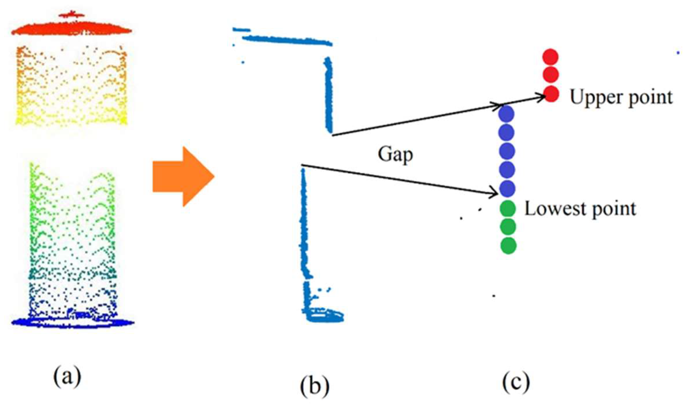
Figure 5.
Gap-filling strategy. (a) Tower point cloud. (b) Vertical cross-section. (c) Red points are the gap’s upper points, green points are the gap’s lowest points, and blue points are points filled inside the gap.
Figure 5.
Gap-filling strategy. (a) Tower point cloud. (b) Vertical cross-section. (c) Red points are the gap’s upper points, green points are the gap’s lowest points, and blue points are points filled inside the gap.

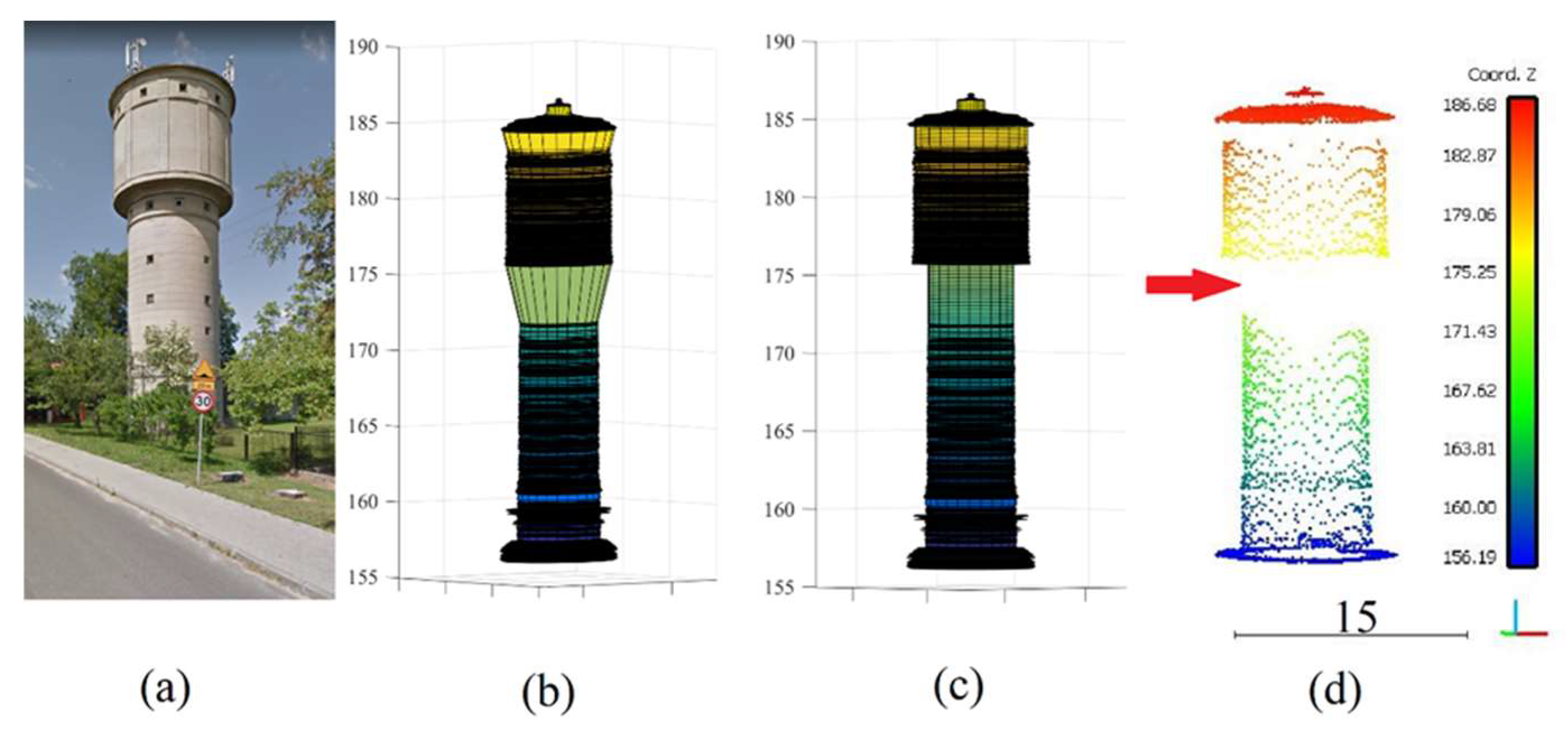
Figure 6.
(a) Tower image. (b)Tower model before filling the gaps. (c) Tower model after filling the gaps. (d) Building point cloud; Red arrow shows gap.
Figure 6.
(a) Tower image. (b)Tower model before filling the gaps. (c) Tower model after filling the gaps. (d) Building point cloud; Red arrow shows gap.

Figure 7.
Vertical spacing between consecutive vertical cross-section points shown in Figure 3a.
Figure 7.
Vertical spacing between consecutive vertical cross-section points shown in Figure 3a.

Figure 8.
Models calculated from the point cloud shown in Figure 2b. (a) Tower model before fillingthe gaps. (b) Tower model after filling the gaps. (c) Tower model after considering all cloud points. (d) Tower image.
Figure 8.
Models calculated from the point cloud shown in Figure 2b. (a) Tower model before fillingthe gaps. (b) Tower model after filling the gaps. (c) Tower model after considering all cloud points. (d) Tower image.

Figure 9.
Integration of a new point within the constructed building model, Ro is the rotating origin, g is the gravity center, and P is a point off the rotating surface.
Figure 9.
Integration of a new point within the constructed building model, Ro is the rotating origin, g is the gravity center, and P is a point off the rotating surface.

Figure 10.
(a) Tower model before including deviated points. (b) Tower model after including deviated points. (c) Laying out point cloud over the tower model after including the deviated points; LiDAR point cloud is in red color.
Figure 10.
(a) Tower model before including deviated points. (b) Tower model after including deviated points. (c) Laying out point cloud over the tower model after including the deviated points; LiDAR point cloud is in red color.

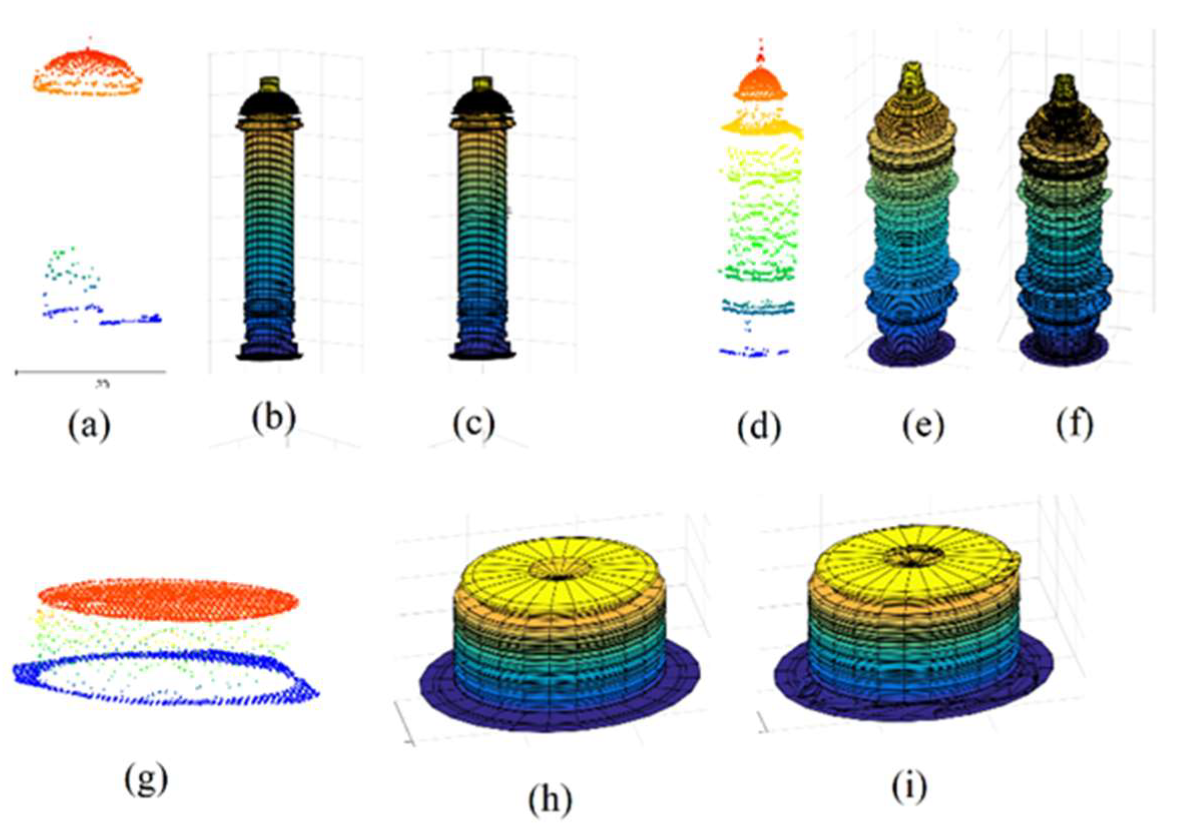
Figure 11.
(a,e,i) Tower images. (b,f,j) Tower point clouds. (c,g,k) Tower model before considering all cloud points. (d,h,l) Tower model after considering all cloud points.
Figure 11.
(a,e,i) Tower images. (b,f,j) Tower point clouds. (c,g,k) Tower model before considering all cloud points. (d,h,l) Tower model after considering all cloud points.

Figure 12.
(a,d,g) Tower point clouds. (b,e,h) Tower model before considering all cloud points. (c,f,i) Tower model after considering all cloud points.
Figure 12.
(a,d,g) Tower point clouds. (b,e,h) Tower model before considering all cloud points. (c,f,i) Tower model after considering all cloud points.


Table 1.
Accuracy of building models for .
| Building Number | Min CW (m) | Max CW (m) | Mean CW (m) | Min CH (m) | Max CH (m) | Mean CH (m) |
|---|---|---|---|---|---|---|
| 1 | 0.01 | 1.36 | 0.81 | 0.01 | 0.20 | 0.02 |
| 2 | 0.01 | 4.55 | 2.79 | 0.01 | 0.20 | 0.01 |
| 3 | 0.02 | 0.66 | 0.40 | 0.01 | 0.20 | 0.07 |
| 4 | 0.01 | 0.88 | 0.53 | 0.01 | 0.20 | 0.08 |
| 5 | 0.01 | 0.49 | 0.26 | 0.01 | 0.20 | 0.04 |
| 6 | 0.01 | 1.33 | 0.75 | 0.01 | 0.14 | 0.02 |
Disclaimer/Publisher’s Note: The statements, opinions and data contained in all publications are solely those of the individual author(s) and contributor(s) and not of MDPI and/or the editor(s). MDPI and/or the editor(s) disclaim responsibility for any injury to people or property resulting from any ideas, methods, instructions or products referred to in the content. |
© 2023 by the authors. Licensee MDPI, Basel, Switzerland. This article is an open access article distributed under the terms and conditions of the Creative Commons Attribution (CC BY) license (https://creativecommons.org/licenses/by/4.0/).
Share and Cite
MDPI and ACS Style
Tarsha Kurdi, F.; Lewandowicz, E.; Gharineiat, Z.; Shan, J. Modeling Multi-Rotunda Buildings at LoD3 Level from LiDAR Data. Remote Sens. 2023, 15, 3324. https://0-doi-org.brum.beds.ac.uk/10.3390/rs15133324
AMA Style
Tarsha Kurdi F, Lewandowicz E, Gharineiat Z, Shan J. Modeling Multi-Rotunda Buildings at LoD3 Level from LiDAR Data. Remote Sensing. 2023; 15(13):3324. https://0-doi-org.brum.beds.ac.uk/10.3390/rs15133324
Chicago/Turabian StyleTarsha Kurdi, Fayez, Elżbieta Lewandowicz, Zahra Gharineiat, and Jie Shan. 2023. "Modeling Multi-Rotunda Buildings at LoD3 Level from LiDAR Data" Remote Sensing 15, no. 13: 3324. https://0-doi-org.brum.beds.ac.uk/10.3390/rs15133324
Note that from the first issue of 2016, this journal uses article numbers instead of page numbers. See further details here.