Article

Small Field Plots Can Cause Substantial Uncertainty in Gridded Aboveground Biomass Products from Airborne Lidar Data

by
K. C. Cushman
1,*,
Sassan Saatchi
1,
Ronald E. McRoberts
2,3,
Kristina J. Anderson-Teixeira
4,5,
Norman A. Bourg
4,
Bruce Chapman
1,
Sean M. McMahon
5,6 and
Christopher Mulverhill
1,7
1
Jet Propulsion Laboratory, California Institute of Technology, Pasadena, CA 91011, USA
2
Raspberry Ridge Analytics, Hugo, MN 55038, USA
3
Department of Forest Resources, University of Minnesota, Saint Paul, MN 55108, USA
4
Conservation Ecology Center, Smithsonian’s National Zoo and Conservation Biology Institute, Front Royal, VA 22630, USA
5
Forest Global Earth Observatory, Smithsonian Tropical Research Institute, Panama City 0843-03092, Panama
6
Smithsonian Environmental Research Center, Edgewater, MD 21037, USA
7
Department of Forest Resources Management, University of British Columbia, Vancouver, BC V6T 1Z4, Canada
*
Author to whom correspondence should be addressed.
Remote Sens. 2023, 15(14), 3509; https://0-doi-org.brum.beds.ac.uk/10.3390/rs15143509
Submission received: 6 May 2023 / Revised: 2 June 2023 / Accepted: 5 June 2023 / Published: 12 July 2023
(This article belongs to the Special Issue NISAR Global Observations for Ecosystem Science and Applications)

Abstract

:
Emerging satellite radar and lidar platforms are being developed to produce gridded aboveground biomass (AGB) predictions that are poised to expand our understanding of global carbon stocks and changes. However, the spatial resolution of AGB map products from these platforms is often larger than the available field plot data underpinning model calibration and validation efforts. Intermediate-resolution/extent remotely sensed data, like airborne lidar, can serve as a bridge between small plots and map resolution, but methods are needed to estimate and propagate uncertainties with multiple layers of data. Here, we introduce a workflow to estimate the pixel-level mean and variance in AGB maps by propagating uncertainty from a lidar-based model using small plots, taking into account prediction uncertainty, residual uncertainty, and residual spatial autocorrelation. We apply this workflow to estimate AGB uncertainty at a 100 m map resolution (1 ha pixels) using 0.04 ha field plots from 11 sites across four ecoregions. We compare uncertainty estimates using site-specific models, ecoregion-specific models, and a general model using all sites. The estimated AGB uncertainty for 1 ha pixels increased with mean AGB, reaching 7.8–33.3 Mg ha−1 for site-specific models (one standard deviation), 11.1–28.2 Mg ha−1 for ecoregion-specific models, and 21.1–22.1 Mg ha−1 for the general model for pixels in the AGB range of 80–100 Mg ha−1. Only 3 of 11 site-specific models had a total uncertainty of <15 Mg ha−1 in this biomass range, suitable for the calibration or validation of AGB map products. Using two additional sites with larger field plots, we show that lidar-based models calibrated with larger field plots can substantially reduce 1 ha pixel AGB uncertainty for the same range from 18.2 Mg ha−1 using 0.04 ha plots to 10.9 Mg ha−1 using 0.25 ha plots and 10.1 Mg ha−1 using 1 ha plots. We conclude that the estimated AGB uncertainty from models estimated from small field plots may be unacceptably large, and we recommend coordinated efforts to measure larger field plots as reference data for the calibration or validation of satellite-based map products at landscape scales (≥0.25 ha).

Graphical Abstract

1. Introduction

Global estimates of the aboveground woody biomass density (AGB) and the changes in AGB over time are important for understanding how climate and land use change affect the global carbon cycle [1]. Multiple current or upcoming spaceborne missions will support the production of global or near-global gridded AGB products. Notably, AGB estimation is an objective for the Global Ecosystem Dynamics Investigation (GEDI) lidar instrument on the International Space Station [2], the Biomass P-band synthetic aperture radar (SAR) satellite [3], and the NASA-ISRO Synthetic Aperture Radar (NISAR) L- and S-band SAR satellite [4]. Together, data from these missions are intended to improve our understanding of AGB carbon stocks and fluxes.
Broad-scale gridded AGB products based on remotely sensed data are estimates produced by models that are calibrated using field data. Among these field data, generally, individual tree size and species observations from forest plots are used to predict biomass using allometric models and are then aggregated to estimate plot-level average AGB. However, the spatial resolution of forest plots is often smaller than the spatial resolution of gridded AGB products, which is constrained by instrument and sampling properties. For example, GEDI, Biomass, and NISAR will support gridded AGB products at 100 ha, 4 ha, and 1 ha, respectively [2,3,4]. These missions will rely largely on contributed plot data collected for other efforts from different vegetation types globally, which are often less than 1 ha in size. Geolocation errors in plots and satellite pixels and the side-looking configuration of radar imagery can cause substantial errors in relating ground measurements of biomass to lidar and radar observations directly [5,6]. Therefore, the direct use of field plots for the calibration and validation of spaceborne missions may introduce large uncertainty to both local predictions and the predicted regional spatial distribution of AGB [7,8].
To address this challenge, NISAR will use airborne laser scanning (ALS) data to scale up field data from smaller, sparse field plots and create 1 ha resolution, landscape-scale AGB estimates that can be used for the calibration of biomass algorithms and validation of NISAR’s AGB estimates [9]. In this approach, fine-resolution (<1 m point spacing) ALS data, as the so-called “gold standard” remote sensing technology for AGB estimation, are combined with the ground-estimated AGB in a model to estimate the AGB at the resolution of forest plots across the entire landscape [10]. ALS-based AGB estimates are then aggregated to provide estimates of the AGB in 1 ha grid cells to match the NISAR AGB product pixel size [11,12,13]. This process removes the large error associated with the direct use of plot data caused by mismatches in the size and location of plots with respect to radar imagery. However, this process also introduces additional sources of uncertainty related to the ALS-based model used to predict AGB and the resampling of ALS AGB pixels to 1 ha grid cells [14,15,16]. In particular, multiple studies have found that uncertainty in AGB-ALS models decreases with increasing plot size, as some sources of error become less important, including spatial mismatches between tree crowns and trunks, and plot/tree geolocation errors [8,12,17,18].
To estimate uncertainty in AGB predictions from NISAR, it is necessary to rigorously account for all sources of errors and to propagate uncertainty from ground plots to ALS and to radar-based estimations of biomass. NISAR’s biomass Algorithm Theoretical Basis Document and Calibration and Validation (“CAL/VAL”) Plan describes the process of the ALS-assisted calibration and validation of the NISAR AGB algorithm [9,19].
In this paper, we develop a workflow to estimate the 1 ha pixel-level uncertainty in AGB predictions associated with scaling AGB estimates from small field plots to larger landscapes with the aid of ALS data, an intermediate step in the NISAR CAL/VAL methodology. We apply a modified version of the methodology outlined in McRoberts et al. to the practical example of producing reference AGB maps, and associated uncertainty maps, using a set of 13 sites in temperate forests across four ecoregions of North America [20]. To properly characterize uncertainty, we also examine: (1) how uncertainty can be reduced by using site-specific or multi-site models associated with similar vegetation types in terms of structure and species and (2) the effect of plot size on the model prediction accuracy. To achieve this goal, we focus on incorporating uncertainty associated with prediction uncertainty and residual variability [20]. Prediction uncertainty is due to the presence of incomplete or imperfect information in the sample data used to train and evaluate models, and residual variability is associated with the distribution of training data around the model predictions.

2. Methods

2.1. Study Sites

We used data from 13 sites in the National Ecological Observation Network (NEON). These sites are distributed across four North American ecoregions (boreal forests, conifer forests, temperate broadleaf/mixed forests, and temperate grasslands/savannas); the ecoregions were defined according to the NISAR mission AGB calibration/validation plan (Figure 1; Table 1) [9]. These study sites were chosen because they contained areas relevant for NISAR AGB estimation (<100 Mg ha−1; BONA, DEJU, OSBS, NIWO, RMNP, TREE, CLBJ, and UKFS), were covered by the 2018 UAVSAR (Uninhabited Aerial Vehicle Synthetic Aperture Radar) campaign to support NISAR algorithm development (LENO, ORNL, and TALL), and/or had co-located large forest dynamics “megaplots” associated with the Smithsonian Forest Global Earth Observatory (ForestGEO) network (SERC, SCBI) [21,22,23].

2.2. Field Estimates of AGB

We estimated the AGB in NEON plots using woody plant vegetation structure data (DP1.10098) from field surveys [24]. We used all plots with recorded tree and sapling data. NEON uses two types of field plots for woody vegetation structure, “distributed plots” and “tower plots”. Both distributed and tower plots are nominally 40 × 40 m in size (0.16 ha), but distributed and tower plots have different subplot sizes where trees are actually measured. In the distributed plots, all trees ≥10 cm in diameter at breast height (DBH) were measured (diameter, species, and stem location) in only one 20 × 20 m (0.04 ha) subplot, while in tower plots, trees are measured in either one or two subplots of 0.04 ha, depending on the vegetation type. At the LENO site, we performed additional fieldwork to measure trees in all four 0.04 ha subplots. To ensure consistency in the sampled area across plot types, all analyses with NEON plot data used 0.04 ha subplots.
Small trees (1 cm ≤ DBH < 10 cm) were also measured in nested subplots large enough to include at least 20 individuals, or throughout the entire plot when small trees were sparse. Our analysis included trees that were ≥2.5 cm DBH, and we estimated the AGB density of small trees by assuming that nested subplots were representative of their plots.
We also estimated the AGB in two ForestGEO megaplots at SCBI and SERC that were 25.6 and 16 ha in size, respectively. In ForestGEO plots, all trees that were ≥1 cm DBH were measured throughout the plot area. We estimated the AGB density in gridded subplots of either 0.04 ha or 1.0 ha, and also included trees that were ≥2.5 cm in our analysis.
For each measured tree, we used allometric models to predict the AGB from the DBH and species the ‘allodb’ package in R. This package predicts AGB using multiple allometries and weights allometric model predictions based on the geographic location of plots [25]. We chose this package because it included allometries based on species included in 24 extratropical megaplots in North America, Europe, and Asia, and allowed consistent AGB predictions across other extratropical NISAR calibration/validation sites. All AGB predictions from ground measurements and allometries were assumed to have no uncertainty; previous studies have found that the effects of allometric model prediction uncertainty are negligible relative to other sources of variability [26,27].

2.3. ALS Data

To scale AGB estimates from field plots to landscapes, we used small-footprint ALS data from the NEON Airborne Observation Platform (AOP). The NEON AOP carries an Optech Gemini ALS sensor and collects data over at least 10,000 ha at each site, with a point density of at least 5.2 pts m−2 (Table 1). For most sites, we used the most recent available ALS data at the time of analysis. For LENO, ORNL, and TALL, we used the ALS data closest in time to the UAVSAR campaigns detailed elsewhere in this special issue. We used the NEON-classified ALS data and excluded points classified as noise (DP1.30003.001) [28].
We processed ALS data into gridded canopy height models using the ‘lidR’ package in R [29,30]. First, we calculated the normalized height above ground for each point with the ‘normalize_height’ function using the k-nearest neighbor approach with inverse-distance weighting. Next, we predicted canopy height with the ‘grid_canopy’ function at a 1 m resolution, using the points-to-raster method to select the tallest ALS return in each pixel with a 0.2 m buffer around the return locations. Last, we predicted the mean canopy height (MCH) as the average of the canopy height values within a larger area, either 0.04 ha plot boundaries or gridded across the landscape at 0.04 ha spatial grain.

2.4. AGB-ALS Model

We used a power function to describe the relationship between the plot-estimated AGB and forest structure (MCH) from ALS data:
A G B = a 1 M C H b 1 + ϵ
where a1 and b1 are the parameters to be estimated and ϵ   ~ N 0 , σ 2 is a random residual term. The power function was fit with the least-squares approach using the ‘nls’ function in R and the Gauss–Newton algorithm. Models were fit using weighted least squares because the AGB prediction residuals were heteroscedastic [20]. The weights were the inverse of the predicted residual variance, where residual variance was predicted using the procedure outlined in [20] for estimating heteroscedastic residual variance:
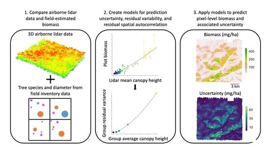
  • First, the plots were ordered by their MCH and sorted into equal-sized groups of at least 10 plots each;
  • Next, the average MCH and biomass residual variance were calculated for each group;
  • Finally, a model was fit describing the increase in residual variance as a power function of average MCH:
σ R V 2 = a 2 M C H - b 2 + δ
where σ R V 2 is the group average residual variance, M C H - is the group average MCH, a2 and b2 are the parameters to be estimated, and δ   ~ N 0 , σ 2 is a random residual term.
The model prediction of σ R V 2 was used to estimate the residual variance for each sample unit (training data) observation.
As weights depended on the fitted model, we used an iterative approach, first fitting Equation (1) without weights and then iteratively refitting using new weights until the estimates of parameters a1 and b1 both varied by less than 1% across five successive iterations.
We fit a single model first, hereafter the “general model”, using AGB and MCH data from all plots at all sites. Next, we fit ecoregion-specific and site-specific models by using the relationship between MCH and AGB for all plots within an ecoregion and site, respectively. We evaluated the initial model fit at each site by reporting the root-mean-square error (RMSE) and R2 of Equation (1) using 10-fold cross-validation—plots were randomly divided into 10 groups and the AGB for each plot was predicted from a model trained only on the other nine groups. All subsequent calculations using Equation (1) residual values were performed using each plot’s residual value from 10-fold cross-validation.

2.5. Predicted Gridded Biomass across Landscapes

We predicted AGB at the landscape scale for each site by applying Equation (1), parameterized with field plot data, to gridded ALS-derived MCH data of the same spatial resolution (0.04 ha). We produced three maps of predicted AGB for each site by applying the general model, the relevant ecoregion-specific model, and the site-specific model [31,32,33]. We predicted AGB at the 1 ha spatial resolution of the NISAR biomass product by first applying the Equation (1) estimated parameters to 0.04 ha resolution pixels (Tables S1 and S2) and then using the ‘aggregate’ function in the ‘raster’ package, taking the mean value of 25 contiguous pixels [34].

2.6. Estimating AGB Uncertainty at 1 ha Resolution

The variance (uncertainty) of the 1 ha gridded mean AGB was estimated using three separate variances associated with the prediction uncertainty, residual variability, and residual spatial autocorrelation:
σ ^ T o t a l 2 = σ ^ P U 2 + σ ^ R V 2 + σ ^ R S A 2
where σ ^ T o t a l 2 is the total estimated uncertainty, σ ^ P U 2 is the prediction uncertainty, σ ^ R V 2 is the residual variability, and σ ^ R S A 2 is the uncertainty associated with the residual spatial autocorrelation.
Prediction uncertainty. We estimated the prediction uncertainty using a “wild bootstrapping” approach [31,32], where the value for each field plot AGB observation was resampled for each bootstrap iteration:
y i , j = y ^ i + ε i ν i , j
where y i , j is the resampled AGB value for plot i and iteration j, y ^ i is the predicted AGB value for plot i from Equation (1), ε i is the residual value for plot i from Equation (1), and ν i , j is randomly selected from a standard normal distribution with mean 0 and standard deviation 1 for each plot i and iteration j. Iterations continued until the standard deviation in the mean estimated landscape AGB across all iterations varied by less than 0.5% compared with the standard deviation of the mean estimated landscape AGB calculated for the preceding 50% of iterations [33]. An example of the distribution of model parameter estimates from bootstrapping is provided in Figure S1. For each 1 ha pixel, σ ^ P U 2 was estimated as the variance in the predicted biomass (at 1 ha spatial grain) across all bootstrap iterations.
Residual uncertainty. The residual variance was calculated for each 0.04 ha pixel ( σ ^ R V , 0.04   h a 2 ) from the MCH using the approach from [20] and described above for estimating residual variance during iterative weighted model fitting (Equation (2); Figures S2 and S3). The residual variance of AGB for each 1 ha grid cell ( σ ^ R V 2 ) was then estimated as:
σ ^ R V 2 = 1 n 2 i = 1 n σ ^ R V , 0.04   h a i 2
where n = 25, the total number of 0.04 ha pixels within each 1 ha pixel.
Residual spatial autocorrelation uncertainty. We estimated the variance from residual spatial autocorrelation using a correlogram constructed from observed model residual values. We constructed the empirical correlogram using two steps. First, we used the ‘correlog’ function from the ‘ncf’ package in R to estimate point values describing the correlation of model residuals for plots at different distances apart, with 20 m distance increments to match the spatial grain of the field plot data [35]. Next, we fit a spline with 3 degrees of freedom to the empirical correlogram data so that the spatial correlation could be predicted at any distance (Figure S4). Owing to the limited number of field plots and the amount of data required to estimate the spatial autocorrelation, we constructed one empirical correlogram from the observed residual values from the general model for all plots and sites combined; we assumed that the magnitude and distance of the spatial autocorrelation did not vary among sites. We estimated the residual spatial autocorrelation for each 1 ha pixel ( σ ^ R S A 2 ) by considering the sum of the products of the residual standard deviations and spatial correlations for each pair of 0.04 ha subpixels:
σ ^ R S A 2 = 1 n 2 i n j = 1 n σ ^ R V , 0.04   h a i σ ^ R V , 0.04   h a j ρ ^ i j
where ρ ^ i j is the correlation between the residuals for the pairs of pixels predicted from the distance between the pixels using the empirical correlogram and n = 25, the total number of 0.04 ha pixels within each 1 ha pixel.

2.7. The Effect of Plot Size on AGB Uncertainty

To explore the relationship between field plot size and uncertainty in the 1 ha resolution gridded AGB products, we leveraged the SCBI and SERC megaplots that allowed us to fit AGB-ALS models at multiple resolutions—we compared the 1 ha pixel-level estimates of uncertainty for models scaled up from 0.04 ha subplots and 0.25 ha subplots, and for models directly fit with 1 ha subplots. As the SCBI and SERC megaplots contained no subplots smaller than 100 Mg ha−1 AGB at 1 ha resolution, we added additional simulated smaller-biomass data by randomly selecting MCH values between 0 and 20 m and AGB predictions based on the AGB-MCH model (Equation (1)) and the residual variance model (Equation (2)), assuming that the models fit to real plot data would predict the relationship for smaller MCH subplots (Figure S5). Ten hectares of additional plot data were simulated for each resolution, keeping the total plot area constant across models of different plot sizes. For each plot size, we calculated estimates of the AGB and associated uncertainty at a 1 ha resolution as described above. When estimating models directly from 1 ha field plots, the pixel-level uncertainty estimates did not include a contribution from residual spatial autocorrelation.

3. Results

3.1. Plot-Based Biomass Estimates

We used 529 plots of 0.04 ha from 11 sites (excluding megaplot sites SCBI and SERC) to compare the performance of general, ecosystem-specific, and site-specific AGB-ALS models, and to demonstrate our upscaling approach. The plot-based biomass estimates ranged from 0.01 to 827.2 Mg ha−1. The large biomass range was mostly due to the small size of the plots and the diversity of sites across temperate broadleaf and mixed forests with greater biomass (ORNL and LENO) and the boreal (DEJU) and temperate conifer (OSBS) sites with smaller biomass (Table 1; Figure 2).

3.2. Plot-Based Model Performance

The general model, describing the relationship between the AGB and MCH in 0.04 ha inventory plots for all sites, had RMSE = 68.4 Mg ha−1 using 10-fold cross-validation.
The relationships between AGB and MCH varied among ecoregions (Figure 2). Ecoregion-specific AGB-MCH models reduced the RMSE for all ecoregions (Table 2). However, the magnitude of RMSE reduction varied among ecoregions, from <2% for the grassland and savanna ecoregions to 20% for boreal forests.
The relationships between AGB and MCH also varied among sites (Figure 3). At the site level, the ecoregion-specific or site-specific model RMSE differed from the general model RMSE by up to 67% for the NIWO site. However, more specific models did not universally reduce the site-level RMSE—depending on the site, either the general, ecoregion-specific, or site-specific model had the smallest RMSE (Table 3).

3.3. One-Hectare-Resolution Estimates of Uncertainty

To characterize how pixel-level uncertainty in the 1 ha gridded AGB estimates varied across sites, among models (general, ecoregion-specific, or site-specific), and for different AGB values, we estimated the average pixel-level uncertainty for each site and model for all pixels in three different AGB ranges chosen to include the AGB range of NISAR’s AGB validation requirement (≤100 Mg ha−1): 0–20 Mg ha−1, 40–60 Mg ha−1, and 80–100 Mg ha−1. For all sites and models, the total uncertainty increased in magnitude with increasing predicted AGB, from 1.1–12.8 Mg ha−1 for pixels with AGB ≤ 20 Mg ha−1, 6.1–28.3 for pixels with AGB 40–60 Mg ha−1, and 7.8–33.3 for pixels with AGB 80–100 Mg ha−1 (Figure 4). The total uncertainty was smallest for the site-specific models in conifer forest sites, for the ecoregion-specific models in temperate broadleaf/mixed forest sites and boreal forest sites, and for the general model in temperate grassland/savanna sites (Figure 4).
We also characterized the relative contribution of each uncertainty component (prediction uncertainty, residual variability, and spatial autocorrelation in residuals) to the total model uncertainty (Figure 5). Residual spatial autocorrelation dominated the total model uncertainty for the general model across all levels of predicted AGB (Figure 5a,d,g), contributing ~70–90% of the total uncertainty; residual variability had the second-largest contribution to the total uncertainty for the general model. The prediction uncertainty was relatively more important for pixels with a smaller predicted AGB in ecoregion-specific models, contributing up to ~80% of the total uncertainty for temperate broadleaf/mixed forest sites and ~50% for temperate grassland/savanna sites (Figure 5b,e,h). The relative contributions among uncertainty components were more variable for site-level models across the range of predicted AGB, although residual variability was consistently smaller than ~50%, while prediction uncertainty and residual spatial autocorrelation could reach up to ~100% and ~80%, respectively, depending on the site (Figure 5c,f,i).

3.4. Plot Size Effects on Gridded AGB Uncertainty

The pixel-level prediction uncertainty, residual uncertainty, and residual spatial autocorrelation uncertainty were all greater for the models estimated from 0.04 ha plots than for the models estimated from 0.25 ha plots and 1 ha plots (Figure 6). The prediction uncertainty and residual uncertainty were the smallest for 0.25 ha plots, but the 1 ha plots had the smallest total pixel-level uncertainty due to the lack of contribution from residual spatial autocorrelation uncertainty. For pixels with AGB 80–100 Mg ha−1 AGB at SCBI and SERC, the average total uncertainty ( σ ^ T o t a l ) for AGB estimates for 1 ha plots was 10.1 Mg ha−1, 45% less than the average for 0.04 ha plots (18.2 Mg ha−1); the average for AGB estimates for 0.25 plots (10.9 Mg ha−1) was 40% less than that for 0.04 ha plots.

4. Discussion

We demonstrated that the pixel-level total uncertainty of gridded AGB products estimated from field plots and ALS data could be substantial compared with predicted AGB values. When ALS is used as an intermediate step in gridded spaceborne AGB product calibration, the uncertainty in ALS and plot-based AGB will influence the uncertainty of the resulting spaceborne product as well.
In this analysis, relatively large uncertainty could be attributed, in part, to the sparse and small field plots. Other studies have also demonstrated that the RMSE in AGB-MCH models decreases with increasing plot area [8,12,17]. While small plots may be efficient and sufficient for other research purposes in forest ecology, larger plots are preferable for reducing uncertainty in model-based remote sensing products, particularly those from spaceborne sensors.
To demonstrate this point, we used the examples of the SCBI and SERC megaplots to develop AGB-MCH models from different plot sizes. We show, in Figure 6, that field plots ≥ 0.25 ha in size are necessary to reduce the uncertainty of lidar-estimated AGB and allow the estimates to be useful for the calibration and validation of other sensors, such as NISAR. The relationship between plot size and lidar model prediction uncertainty likely varies among ecoregions, and plots < 0.25 ha (but larger than 0.04 ha, based on our results) may be acceptable in ecoregions with lower biomass and/or higher stem density of trees (e.g., boreal forests). It can be challenging to know a priori what plot size is needed in a particular context, and ≥0.25 ha is a conservative choice that is likely to be sufficient in most systems. Our recommendations are consistent with the Committee on Earth Observation Satellites aboveground woody biomass working group recommendation of plot sizes of ≥0.25 ha in higher-biomass forests [18].
The model (general, ecoregion-specific, or site-specific) that most reduced the total pixel-level uncertainty varied between sites in this analysis. For example, for all conifer forest sites, the site-specific AGB predictions had less total uncertainty than either the ecoregion-specific or general AGB predictions (Figure 4). However, for the temperate broadleaf/mixed forest sites, total AGB prediction uncertainty was the lowest for the ecoregion model (Figure 4). This occurred because there was more variation in the AGB-MCH relationships among sites for boreal forest sites than for temperate broadleaf/mixed forest sites (Figure 3), resulting in greater residual variance for the boreal ecoregion model compared with the broadleaf/mixed model (Figure S2). When structural differences among sites are less apparent, using ecoregion-specific or general models calibrated with more data can reduce the contribution of prediction uncertainty to the total uncertainty (Figure 5). In addition to the total uncertainty in pixel-level AGB estimates, other considerations may also be important for model choice, such as systematic prediction error or bias (Figure S6).
There may be practical challenges to applying this framework to rigorously estimate model prediction uncertainty resulting from the volume of data needed to estimate intermediate model parameters. For example, the model for predicting the residual variance from MCH (Equation (2)) was fit using grouped data, where each group should have ≥10 separate observations. Therefore, at least 30 observations (i.e., field plots) were required to fit Equation (2)—having insufficient data to properly fit this model could result in inaccurate estimates of residual variation. Estimation of the correlogram—describing the correlation between residual values among plots/pixels as a function of distance—requires not only a large number of field plots, but also field plots that are arranged in space across an appropriate range of distances, particularly small distances, where the spatial autocorrelation is greatest. Here, we assumed that one empirical correlogram was applicable to all sites and models. The correlograms were likely to have varied among sites, but we lacked the data to fit site-specific correlograms.
We acknowledge approaches that could potentially further reduce the total model prediction uncertainty. For example, including additional ALS metrics, such as alternative height or canopy cover metrics, can improve the performance of AGB-ALS models for some ecoregions [36]. We limited this analysis to the mean top of canopy height, because this metric tends to be relatively stable across instrument and data collection characteristics [37]. Further, improving field plot and ALS co-registration can reduce uncertainty in field plot ALS models—one example using National Forest Inventory data from Spain found that increasing the accuracy of field plot geolocation reduced the RMSE of models predicting the stand volume and basal area by ~10% [38]; another study found that using survey-grade global positioning system (GPS) receivers with sub-meter accuracy reduced the standard error of large-area AGB estimates by over 20% compared with GPS receivers with location errors of up to 5–10 m [39]. In this framework, models with additional parameters may reduce residual variability, but may also increase prediction uncertainty; the overall effect on the total uncertainty of adding additional metrics and parameters warrants further study. Here, we also assumed that the species-level AGB-diameter allometries exhibited no systematic prediction error. These allometries can have large uncertainties for individual trees (particularly large trees); therefore, the plot-level AGB for small plots can be uncertain as well, contributing to large residual variations [18,40]. Although other approaches can be more accurate for individual tree AGB estimation (such as terrestrial lidar), these data are not yet widely available for landscape-level applications due to current limitations in data collection and processing at scale [41]. Therefore, using ALS-based AGB estimates is necessary at this time to obtain enough 1 ha AGB samples to train and test SAR models, and to avoid errors associated with geolocation mismatches between field plots and satellite pixels [5,6].
This analysis is meant to demonstrate the workflow that will be applied for constructing gridded reference AGB products for the calibration and validation of the NISAR mission—the actual AGB estimates and associated uncertainty for NEON sites are likely to change from additional data collection before NISAR’s launch and calibration/validation period. Our results support recent calls to have consistent, high-quality field data for the cal/val of remote sensing AGB products and large-scale Earth system models [13,42,43,44].

5. Conclusions

We provide a framework for estimating pixel-level uncertainty in gridded products from AGB-lidar models; this framework will be used as part of the calibration/validation effort for the NISAR AGB algorithm.
The uncertainty of predicted AGB from ALS increases in absolute values with AGB, and varies among sites depending on whether the AGB-MCH model is developed based on site-specific, ecoregion-specific, or general (using all sites/ecoregions) data.
Our results show that plot size has a substantial impact on the uncertainty of AGB predicted from ALS data. Predictions from models created using small field plots have large uncertainty due to several factors, among them including the uncertainty of ground-estimated biomass in small plots, difficulty of height capturing the variability of volume and tree size, potential extension of tree crowns outside the lidar pixels of plot area, and potential plot location errors. Larger field plots can reduce the uncertainty of AGB predicted from lidar height metrics. We recommend large (≥0.25 ha) field plots for use in developing AGB-lidar models with reasonably low uncertainty.

Supplementary Materials

The following supporting information can be downloaded at: https://0-www-mdpi-com.brum.beds.ac.uk/article/10.3390/rs15143509/s1. Figure S1. Parameter estimates for MCH-AGB models (Equation (1)) for the BONA site. Figure S2. Fitted models describing residual variance as a function of canopy height (Equation (2)) for the general model and for each ecoregion-specific model. Figure S3. Fitted models describing residual variance as a function of canopy height (Equation (2)) for each site-specific model within ecoregions. Figure S4. Estimated empirical spatial correlogram describing how the correlation between model residual values changes with distance. Figure S5. Megaplot data from the SCBI and SERC sites used to compare 1-ha pixel-level uncertainty in AGB estimated from 0.04 ha subplots, 0.25 ha subplots, and 1 ha subplots. Figure S6. Differences in predicted AGB using the general, ecoregion-specific, or site-specific models for each site (Equation (1)). Table S1. Equation (1) estimated parameters used for AGB prediction for 0.04 ha pixels from NEON plot data. Table S2. Equation (1) estimated parameters used for AGB prediction for pixels of varying size from ForestGEO plot data at SERC and SCBI (combined).

Author Contributions

Conceptualization, S.S. and K.C.C.; Data curation, K.C.C., K.J.A.-T., N.A.B., S.M.M. and C.M.; Formal analysis, K.C.C. and C.M.; Funding acquisition, S.S. and B.C.; Methodology, K.C.C., S.S. and R.E.M.; Software, K.C.C. and C.M.; Supervision, S.S. and B.C.; Visualization, K.C.C.; Writing—original draft, K.C.C.; Writing—review and editing, all authors. All authors have read and agreed to the published version of the manuscript.

Funding

This research was carried out at the Jet Propulsion Laboratory, California Institute of Technology, under a contract with the National Aeronautics and Space Administration (80NM0018D0004). We thank the NISAR mission for supporting this work. The National Ecological Observatory Network is a program sponsored by the National Science Foundation and operated under cooperative agreement by Battelle. This material is based in part upon work supported by the National Science Foundation through the NEON Program. Funding for the Smithsonian Conservation Biology Institute (SCBI) Large Forest Dynamics Plot (LFDP) was provided by the Smithsonian Institution, the National Zoological Park, and the HSBC Climate Partnership.

Data Availability Statement

The data and code underlying results in this study are publicly available at https://0-doi-org.brum.beds.ac.uk/10.48577/jpl.FIAYOG.

Acknowledgments

The SCBI and SERC LFDPs are part of the Smithsonian Institution Forest Global Earth Observatory, a worldwide network of large, long-term forest dynamics plots. Thanks to Bill McShea for his assistance in making the SCBI plot data available.

Conflicts of Interest

The authors declare no conflict of interest.

References

  1. Xu, L.; Saatchi, S.S.; Yang, Y.; Yu, Y.; Pongratz, J.; Anthony Bloom, A.; Bowman, K.; Worden, J.; Liu, J.; Yin, Y.; et al. Changes in Global Terrestrial Live Biomass over the 21st Century. Sci. Adv. 2021, 7, eabe9829. [Google Scholar] [CrossRef]
  2. Dubayah, R.; Armston, J.; Healey, S.; Bruening, J.; Patterson, P.; Kellner, J.; Duncanson, L.; Saarela, S.; Ståhl, G.; Yang, Z.; et al. GEDI Launches a New Era of Biomass Inference from Space. Environ. Res. Lett. 2022, 17, 095001. [Google Scholar] [CrossRef]
  3. Quegan, S.; Le Toan, T.; Chave, J.; Dall, J.; Exbrayat, J.F.; Minh, D.H.T.; Lomas, M.; D’Alessandro, M.M.; Paillou, P.; Papathanassiou, K.; et al. The European Space Agency BIOMASS Mission: Measuring Forest Above-Ground Biomass from Space. Remote Sens. Environ. 2019, 227, 44–60. [Google Scholar] [CrossRef] [Green Version]
  4. Rosen, P.A.; Kumar, R. NASA-ISRO SAR (NISAR) Mission Status. In Proceedings of the 2021 IEEE Radar Conference, Atlanta, GA, USA, 8–14 May 2021; Institute of Electrical and Electronics Engineers Inc.: Atlanta, GA, USA, 2021; pp. 1–6. [Google Scholar]
  5. Shugart, H.H.; Saatchi, S.; Hall, F.G. Importance of Structure and Its Measurement in Quantifying Function of Forest Ecosystems. J. Geophys. Res. Biogeosci 2010, 115, G00E13. [Google Scholar] [CrossRef]
  6. Saatchi, S.; Marlier, M.; Chazdon, R.L.; Clark, D.B.; Russell, A.E. Impact of Spatial Variability of Tropical Forest Structure on Radar Estimation of Aboveground Biomass. Remote Sens. Environ. 2011, 115, 2836–2849. [Google Scholar] [CrossRef]
  7. Xu, L.; Saatchi, S.S.; Shapiro, A.; Meyer, V.; Ferraz, A.; Yang, Y.; Bastin, J.F.; Banks, N.; Boeckx, P.; Verbeeck, H.; et al. Spatial Distribution of Carbon Stored in Forests of the Democratic Republic of Congo. Sci. Rep. 2017, 7, 15030. [Google Scholar] [CrossRef] [PubMed] [Green Version]
  8. Hernández-Stefanoni, J.L.; Reyes-Palomeque, G.; Castillo-Santiago, M.Á.; George-Chacón, S.P.; Huechacona-Ruiz, A.H.; Tun-Dzul, F.; Rondon-Rivera, D.; Dupuy, J.M. Effects of Sample Plot Size and GPS Location Errors on Aboveground Biomass Estimates from LiDAR in Tropical Dry Forests. Remote Sens. 2018, 10, 1586. [Google Scholar] [CrossRef] [Green Version]
  9. Chapman, B.; Rosen, P.; Joughin, I.; Siqueira, P.; Saatchi, S.; Meyer, V.; Borsa, A.; Meyer, F.; Simard, M.; Lohman, R.; et al. NISAR Calibration and Validation Plan V0.9, NASA Jet Propulsion Laboratory Document D-80829; California Institute of Technology: Pasadena, CA, USA, 2018. [Google Scholar]
  10. Næsset, E. Predicting Forest Stand Characteristics with Airborne Scanning Laser Using a Practical Two-Stage Procedure and Field Data. Remote Sens. Environ. 2002, 80, 88–99. [Google Scholar] [CrossRef]
  11. Næsset, E.; Gobakken, T. Estimation of Above- and Below-Ground Biomass across Regions of the Boreal Forest Zone Using Airborne Laser. Remote Sens. Environ. 2008, 112, 3079–3090. [Google Scholar] [CrossRef]
  12. Meyer, V.; Saatchi, S.S.; Chave, J.; Dalling, J.; Bohlman, S.; Fricker, G.A.; Robinson, C.; Neumann, M. Detecting Tropical Forest Biomass Dynamics from Repeated Airborne Lidar Measurements. Biogeosci. Discuss. 2013, 10, 1957–1992. [Google Scholar] [CrossRef] [Green Version]
  13. Duncanson, L.; Armston, J.; Disney, M.; Avitabile, V.; Barbier, N.; Calders, K.; Carter, S.; Chave, J.; Herold, M.; Crowther, T.W.; et al. The Importance of Consistent Global Forest Aboveground Biomass Product Validation. Surv. Geophys. 2019, 40, 979–999. [Google Scholar] [CrossRef] [Green Version]
  14. Frazer, G.W.; Magnussen, S.; Wulder, M.A.; Niemann, K.O. Simulated Impact of Sample Plot Size and Co-Registration Error on the Accuracy and Uncertainty of LiDAR-Derived Estimates of Forest Stand Biomass. Remote Sens. Environ. 2011, 115, 636–649. [Google Scholar] [CrossRef]
  15. Gregoire, T.G.; Ståhl, G.; Næsset, E.; Gobakken, T.; Nelson, R.; Holm, S. Model-Assisted Estimation of Biomass in a LiDAR Sample Survey in Hedmark County, Norway. Canadian J. Forest Res. 2011, 41, 83–95. [Google Scholar] [CrossRef]
  16. McRoberts, R.E.; Næsset, E.; Gobakken, T. Inference for Lidar-Assisted Estimation of Forest Growing Stock Volume. Remote Sens. Environ. 2013, 128, 268–275. [Google Scholar] [CrossRef]
  17. Mascaro, J.; Detto, M.; Asner, G.P.; Muller-Landau, H.C. Evaluating Uncertainty in Mapping Forest Carbon with Airborne LiDAR. Remote Sens. Environ. 2011, 115, 3770–3774. [Google Scholar] [CrossRef]
  18. Duncanson, L.; Armston, J.; Disney, M.; Avitabile, V.; Barbier, N.; Calders, K.; Carter, S.; Chave, J.; Herold, M.; MacBean, N.; et al. Aboveground Woody Biomass Product Validation Good Practices Protocol. In Good Practices for Satellite Derived Land Product Validation; Duncanson, L., Disney, M., Armston, J., Nickeson, J., Minor, D., Camacho, F., Eds.; Land Product Validation Subgroup (WGCV/CEOS), 2021; p. 236. Available online: https://lpvs.gsfc.nasa.gov/PDF/CEOS_WGCV_LPV_Biomass_Protocol_2021_V1.0.pdf (accessed on 4 June 2023). [CrossRef]
  19. NISAR Science Team. NISAR Ecosystems Science Algorithms. Available online: https://gitlab.com/nisar-science-algorithms/ecosystems (accessed on 4 June 2023).
  20. McRoberts, R.E.; Næsset, E.; Saatchi, S.; Quegan, S. Statistically Rigorous, Model-Based Inferences from Maps. Remote Sens. Environ. 2022, 279, 113028. [Google Scholar] [CrossRef]
  21. Davies, S.J.; Abiem, I.; Salim, K.A.; Aguilar, S.; Allen, D.; Alonso, A.; Anderson-Teixeira, K.; Andrade, A.; Arellano, G.; Ashton, P.S.; et al. ForestGEO: Understanding Forest Diversity and Dynamics through a Global Observatory Network. Biol. Conserv. 2021, 253, 108907. [Google Scholar] [CrossRef]
  22. Anderson-Teixeira, K.J.; Davies, S.J.; Bennett, A.C.; Gonzalez-Akre, E.B.; Muller-Landau, H.C.; Joseph Wright, S.; Abu Salim, K.; Almeyda Zambrano, A.M.; Alonso, A.; Baltzer, J.L.; et al. CTFS-ForestGEO: A Worldwide Network Monitoring Forests in an Era of Global Change. Glob. Chang. Biol. 2014, 21, 528–549. [Google Scholar] [CrossRef] [Green Version]
  23. Bourg, N.A.; McShea, W.J.; Thompson, J.R.; McGarvey, J.C.; Shen, X. Initial Census, Woody Seedling, Seed Rain, and Stand Structure Data for the SCBI SIGEO Large Forest Dynamics Plot. Ecology 2013, 94, 2111–2112. [Google Scholar] [CrossRef]
  24. NEON (National Ecological Observatory Network). Vegetation Structure (DP1.10098.001); RELEASE-2022; NEON: Boulder, CO, USA, 2022. [Google Scholar]
  25. Gonzalez-Akre, E.; Piponiot, C.; Lepore, M.; Herrmann, V.; Lutz, J.A.; Baltzer, J.L.; Dick, C.W.; Gilbert, G.S.; He, F.; Heym, M.; et al. Allodb: An R Package for Biomass Estimation at Globally Distributed Extratropical Forest Plots. Methods Ecol. Evol. 2022, 13, 330–338. [Google Scholar] [CrossRef]
  26. McRoberts, R.E.; Westfall, J.A. Effects of Uncertainty in Model Predictions of Individual Tree Volume on Large Area Volume Estimates. Forest Sci. 2014, 60, 34–42. [Google Scholar] [CrossRef]
  27. McRoberts, R.E.; Westfall, J.A. Propagating Uncertainty through Individual Tree Volume Model Predictions to Large-Area Volume Estimates. Ann. For. Sci. 2016, 73, 625–633. [Google Scholar] [CrossRef] [Green Version]
  28. NEON (National Ecological Observatory Network). Discrete Return LiDAR Point Cloud (DP1.30003.001); NEON: Boulder, CO, USA, 2022. [Google Scholar]
  29. Roussel, J.R.; Auty, D.; Coops, N.C.; Tompalski, P.; Goodbody, T.R.H.; Meador, A.S.; Bourdon, J.F.; de Boissieu, F.; Achim, A. LidR: An R Package for Analysis of Airborne Laser Scanning (ALS) Data. Remote Sens. Environ. 2020, 251, 112061. [Google Scholar] [CrossRef]
  30. Roussel, J.-R.; Auty, D. LidR: Airborne LiDAR Data Manipulation and Visualization for Forestry Applications, R. Package Version 3.1.2. 2021. Available online: https://cran.r-project.org/package=lidR (accessed on 4 June 2023).
  31. Liu, R.Y. Bootstrap Procedures under Some Non-I.I.D. Models. Ann. Stat. 1988, 16, 1696–1708. [Google Scholar] [CrossRef]
  32. Wu, C.F.J. Jackknife, Bootstrap and Other Resampling Methods in Regression Analysis. Ann. Stat. 1986, 14, 1261–1350. [Google Scholar] [CrossRef]
  33. McRoberts, R.E.; Næsset, E.; Hou, Z.; Ståhl, G.; Saarela, S.; Esteban, J.; Travaglini, D.; Mohammadi, J.; Chirici, G. How Many Bootstrap Replications Are Necessary for Estimating Remote Sensing-Assisted, Model-Based Standard Errors? Remote Sens. Environ. 2023, 288, 113455. [Google Scholar] [CrossRef]
  34. Hijmans, R.J. Raster: Geographic Data Analysis and Modeling, R. Package Version 2.8-4. 2021. Available online: https://CRAN.R-project.org/package=raster (accessed on 4 June 2023).
  35. Bjornstad, O.N. ncf: Spatial Covariance Functions, R package version 1.3-2. 2022. Available online: https://CRAN.R-project.org/package=ncf (accessed on 4 June 2023).
  36. Lefsky, M.A.; Cohen, W.B.; Harding, D.J.; Parker, G.G.; Acker, S.A.; Gower, S.T. Lidar Remote Sensing of Above-Ground Biomass in Three Biomes. Glob. Ecol. Biogeogr. 2002, 11, 393–399. [Google Scholar] [CrossRef] [Green Version]
  37. Görgens, E.B.; Packalen, P.; da Silva, A.G.P.; Alvares, C.A.; Campoe, O.C.; Stape, J.L.; Rodriguez, L.C.E. Stand Volume Models Based on Stable Metrics as from Multiple ALS Acquisitions in Eucalyptus Plantations. Ann. For. Sci. 2015, 72, 489–498. [Google Scholar] [CrossRef]
  38. Pascual, A.; Guerra-Hernández, J.; Cosenza, D.N.; Sandoval-Altalerrea, V. Using Enhanced Data Co-Registration to Update Spanish National Forest Inventories (NFI) and to Reduce Training Data under LiDAR-Assisted Inference. Int. J. Remote Sens. 2021, 42, 106–127. [Google Scholar] [CrossRef]
  39. McRoberts, R.E.; Chen, Q.; Walters, B.F.; Kaisershot, D.J. The Effects of Global Positioning System Receiver Accuracy on Airborne Laser Scanning-Assisted Estimates of Aboveground Biomass. Remote Sens. Environ. 2018, 207, 42–49. [Google Scholar] [CrossRef]
  40. Burt, A.; Calders, K.; Cuni-Sanchez, A.; Gomez-Dans, J.; Lewis, P.; Lewis, S.L.; Malhi, Y.; Phillips, O.L.; Disney, M. Assessment of Bias in Pan-Tropical Biomass Predictions. Front. For. Glob. Chang. 2020, 3, 1–20. [Google Scholar] [CrossRef] [Green Version]
  41. Demol, M.; Verbeeck, H.; Gielen, B.; Armston, J.; Burt, A.; Disney, M.; Duncanson, L.; Hackenberg, J.; Kükenbrink, D.; Lau, A.; et al. Estimating Forest Above-Ground Biomass with Terrestrial Laser Scanning: Current Status and Future Directions. Methods Ecol. Evol. 2022, 13, 1628–1639. [Google Scholar] [CrossRef]
  42. Labrière, N.; Davies, S.J.; Disney, M.I.; Duncanson, L.I.; Herold, M.; Lewis, S.L.; Phillips, O.L.; Quegan, S.; Saatchi, S.S.; Schepaschenko, D.G.; et al. Toward a Forest Biomass Reference Measurement System for Remote Sensing Applications. Glob. Chang. Biol. 2023, 29, 827–840. [Google Scholar] [CrossRef]
  43. Chave, J.; Davies, S.J.; Phillips, O.L.; Lewis, S.L.; Sist, P.; Schepaschenko, D.; Armston, J.; Baker, T.R.; Coomes, D.; Disney, M.; et al. Ground Data Are Essential for Biomass Remote Sensing Missions. Surv. Geophys. 2019, 40, 863–880. [Google Scholar] [CrossRef]
  44. Clark, D.A.; Asao, S.; Fisher, R.; Reed, S.; Reich, P.B.; Ryan, M.G.; Wood, T.E.; Yang, X. Reviews and Syntheses: Field Data to Benchmark the Carbon-Cycle Models for Tropical Forests. Biogeosciences 2017, 14, 4663–4690. [Google Scholar] [CrossRef] [Green Version]
Figure 1. Location of study sites and the distribution of NISAR ecoregions in the United States and Canada. More detailed information about each study site, including latitude/longitude, is provided in Table 1.
Remotesensing 15 03509 g001
Figure 2. Comparison of the general model relating aboveground woody biomass to the mean canopy height (fit to all data) with ecoregion-specific models. Each point represents one 0.04 ha field inventory plot.
Remotesensing 15 03509 g002
Figure 3. Comparison of the general model (fit to all data), ecoregion-specific models, and site-specific models relating the aboveground woody biomass to mean canopy height. Each point represents one 0.04 ha field inventory plot. Gray points are plot data from other ecoregions, included for comparison.
Remotesensing 15 03509 g003
Figure 4. Variation in the average total pixel-level model uncertainty ( σ ^ T o t a l , Equation (3)) across sites, models (general model, ecoregion-specific models, and site-specific models), and predicted AGB values. Each point represents the average pixel-level uncertainty for a given site for all 1 ha gridded pixels within 1 of 3 predicted AGB ranges: 0–20 Mg ha−1 (a,b), 40–60 Mg ha−1 (c,d), and 80–100 Mg ha−1 (e,f). The left-hand panels (a,c,e) compare uncertainty from the general model (x-axis) with uncertainty from the relevant ecoregion-specific model (y-axis), and the right-hand panels (b,d,f) compare uncertainty from site-specific models (x-axis) with uncertainty from the relevant ecoregion-specific model (y-axis). Each panel includes one point per site, colored by ecoregion.
Remotesensing 15 03509 g004
Figure 5. Ternary plots showing the relative contribution of prediction uncertainty, residual variability, and residual spatial autocorrelation to the total model uncertainty ( σ ^ T o t a l , Equation (3)) among sites and for different AGB ranges. Each point represents the site-level average across all 1 ha pixels with low (0–20 Mg ha−1, ac), medium (40–60 Mg ha−1, df), or high (80–100 Mg ha−1, gi) predicted AGB values within the range of interest (0–100 Mg ha−1) for the NISAR mission. Results are shown for the general model (left column), ecoregion-specific model (center column), or site-specific model (right column) applied to each site.
Remotesensing 15 03509 g005
Figure 6. Variation in prediction uncertainty ( σ ^ P U in Equation (3), a), residual variability ( σ ^ R V in Equation (3), b), residual spatial autocorrelation ( σ ^ R S A in Equation (3), c), and total model uncertainty ( σ ^ T o t a l in Equation (3), d) for 1 ha gridded AGB estimates derived from 0.04 ha, 0.25, ha, or 1 ha subplots at the SCBI and SERC sites with ForestGEO megaplots. Residual spatial autocorrelation does not contribute to the total pixel-level uncertainty of 1 ha plots because the models were fit to the data of the same spatial resolution. All uncertainty values are in absolute units (Mg ha−1).
Remotesensing 15 03509 g006
Table 1. Study sites with the National Ecological Observation Network (NEON). NEON plots were measured for woody vegetation structure on a rotating basis, with a subset of plots at each site measured each year, resulting in a range of years for those data per site.
NISAR EcoregionSite NameLocationPlot DataALS Data
LatitudeLongitudeYearsAGB Mean [Range]
(Mg ha−1)
Area
(ha)
YearDensity
(pts m−2)
Boreal forestsCaribou–Poker Creeks Research Watershed (BONA)63.876−149.2132016–202196.1
[1.5, 149.0]
23,473202116.9
Delta Junction (DEJU)63.881−145.7512016–202120.9
[0.2, 104.6]
19,54320218.2
Conifer forestsOrdway–Swisher Biological Station (OSBS)29.689−81.9932016–202070.2
[16.3, 206.8]
19,394202113.6 *
Niwot Ridge (NIWO)40.054−105.5822015–2020124.7
[0.01, 346.3]
13,68820205.6
Rocky Mountain National Park (RMNP)40.276−105.5462017–2020149.3
[31.8, 275.6]
19,796202011.9 *
Temperate broadleaf and mixed forestsLenoir Landing (LENO)31.854−88.1612017–2021175.8
[0.4, 961.4]
11,48320195.2
Oak Ridge (ORNL)35.964−84.2832017–2018247.6
[0.1, 441.3]
23,910201814.0
Smithsonian Conservation Biology Institute (SCBI) 38.893−78.1392018306.4
[7.2, 758.5]
11,243202114.1 *
Smithsonian Environmental Research Center (SERC) 38.890−76.5602014326.6
[0.8, 1022.3]
10,884202112.8 *
Talladega National Forest (TALL)32.950−87.3932015–2020150.6
[1.3, 328.9]
13,61620196.3
Treehaven (TREE)45.494−89.5862018–2021132.6
[7.9, 265.2]
23,491202013.1 *
Temperate grasslands and savannasLyndon B. Johnson National Grassland (CLBJ)33.368−97.5872016–2021108.7
[0.1, 265.4]
15,794202112.0
University of Kansas Field Station (UKFS)39.040−95.1922016–2020165.9
[10.3, 506.0]
13,591202010.7
* ALS data subsampled from greater point density data; site used to validate the uncertainty propagation method only using ForestGEO megaplot data; mean and range AGB values were based on 0.04 ha subplots of the ForestGEO megaplot.
Table 2. Ecoregion-scale performance of models relating AGB and MCH for 0.04 ha inventory plots. Sites within each ecoregion are given in Table 1. All RMSE values were calculated using 10-fold cross-validation, and are presented in units of AGB and as a percentage of the mean AGB of the respective ecoregion.
EcoregionRMSE
(Mg ha−1)
[% of Mean AGB]
R2Number of Plots
General ModelEcoregion ModelGeneral ModelEcoregion Model
Boreal forests34.7
[61.9]
27.7
[49.5]
0.770.8592
Temperate grasslands and savannas75.0
[53.2]
74.0
[52.5]
0.340.3589
Temperate broadleaf and mixed forests72.8
[41.7]
68.9
[39.4]
0.600.64243
Temperate conifer forests73.8
[68.4]
68.4
[63.4]
0.060.20105
Table 3. Site-scale performance of models relating AGB and MCH for 0.04 ha inventory plots. All RMSE values were calculated using 10-fold cross-validation, and are presented in units of AGB and as a percentage of the mean AGB of the respective site.
EcoregionSiteRMSE
(Mg ha−1)
[% of Mean AGB]
R2Number of Plots
GeneralEcoregionSiteGeneralEcoregionSite
Boreal forestsBONA48.6
[50.5]
38.2
[39.7]
39.5
[41.1]
0.690.810.8043
DEJU13.7
[65.6]
12.9
[61.7]
11.2
[53.4]
0.480.540.6649
Temperate grasslands and savannasCLBJ65.3
[60.1]
55.1
[50.7]
56.2
[51.7]
0.350.540.5239
UKFS81.7
[49.3]
85.9
[51.8]
86.0
[51.8]
0.210.130.1350
Temperate broadleaf and mixed forestsLENO93.9
[53.4]
88.4
[50.3]
95.0
[54.0]
0.640.680.6375
ORNL82.2
[33.2]
83.3
[33.6]
83.8
[33.8]
0.250.230.2352
TALL51.4
[34.1]
48.1
[31.9]
49.3
[32.8]
0.480.550.5257
TREE46.3
[34.9]
35.8
[27.0]
35.9
[27.0]
0.340.610.6159
Temperate conifer forestsNIWO95.4
[76.5]
74.9
[60.1]
31.2
[25.0]
0.000.350.8926
OSBS40.2
[57.3]
62.1
[88.5]
23.9
[34.1]
0.080.000.6747
RMNP90.0
[60.2]
71.5
[47.9]
39.5
[26.4]
0.000.060.7132
Disclaimer/Publisher’s Note: The statements, opinions and data contained in all publications are solely those of the individual author(s) and contributor(s) and not of MDPI and/or the editor(s). MDPI and/or the editor(s) disclaim responsibility for any injury to people or property resulting from any ideas, methods, instructions or products referred to in the content.

