
Attention-Enhanced Generative Adversarial Network for Hyperspectral Imagery Spatial Super-Resolution

School of Electronics and Information, Northwestern Polytechnical University, Xi’an 710129, China
*
Author to whom correspondence should be addressed.
Remote Sens. 2023, 15(14), 3644; https://0-doi-org.brum.beds.ac.uk/10.3390/rs15143644
Submission received: 17 April 2023
/
Revised: 20 May 2023
/
Accepted: 19 July 2023
/
Published: 21 July 2023
(This article belongs to the Special Issue Active Learning Methods for Remote Sensing Image Classification)
Abstract
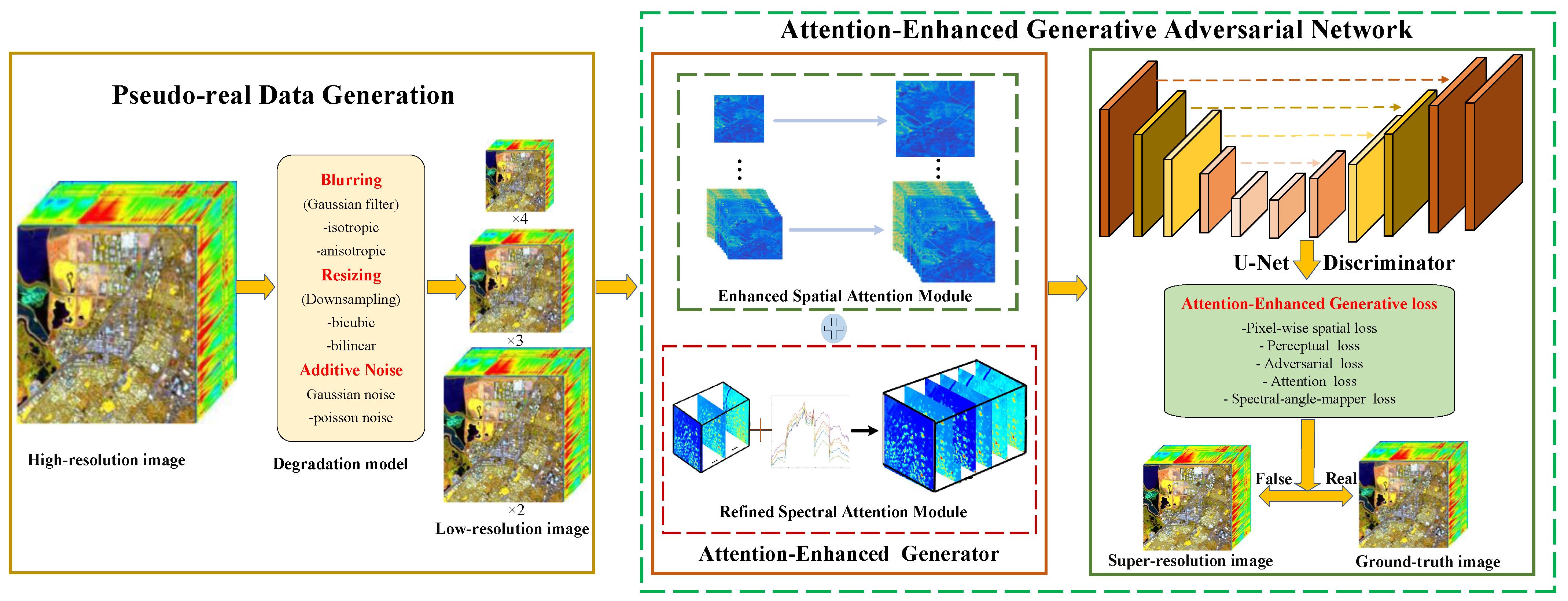
:Hyperspectral imagery (HSI) with high spectral resolution contributes to better material discrimination, while the spatial resolution limited by the sensor technique prevents it from accurately distinguishing and analyzing targets. Though generative adversarial network-based HSI super-resolution methods have achieved remarkable progress, the problems of treating vital and unessential features equally in feature expression and training instability still exist. To address these issues, an attention-enhanced generative adversarial network (AEGAN) for HSI spatial super-resolution is proposed, which elaborately designs the enhanced spatial attention module (ESAM) and refined spectral attention module (RSAM) in the attention-enhanced generator. Specifically, the devised ESAM equipped with residual spatial attention blocks (RSABs) facilitates the generator that is more focused on the spatial parts of HSI that are difficult to produce and recover, and RSAM with spectral attention refines spectral interdependencies and guarantees the spectral consistency at the respective pixel positions. Additionally, an especial U-Net discriminator with spectral normalization is enclosed to pay more attention to the detailed informations of HSI and yield to stabilize the training. For producing more realistic and detailed super-resolved HSIs, an attention-enhanced generative loss is constructed to train and constrain the AEGAN model and investigate the high correlation of spatial context and spectral information in HSI. Moreover, to better simulate the complicated and authentic degradation, pseudo-real data are also generated with a high-order degradation model to train the overall network. Experiments on three benchmark HSI datasets illustrate the superior performance of the proposed AEGAN method in HSI spatial super-resolution over the compared methods.
1. Introduction
Hyperspectral remote sensing imagery provides rich spectral information with tens to hundreds of continuous and narrow electromagnetic spectra of ground object pixels and spatial structure characteristics of an imaging scene [1]. Owing to the physical constraints of sensors and exceedingly high acquisition costs in practice, hyperspectral imagery (HSI) with both high spatial resolution and high spectral resolution cannot be achieved concurrently in remote sensing, which causes difficulties in terms of objective and accurate land cover identification and analysis in HSIs. Hyperspectral image super-resolution (HSI-SR) is conducive to spatial-spectral resolution improvement and the recovery of HSIs from their corresponding low resolution (LR) observations, which is an economic, efficient, and promising signal post-processing technology in remote sensing. And super-resolved HSIs can be widely applied in many fields of computer vision and remote sensing, including object detection [2,3], target recognition [4,5], and land cover classification [6,7,8].
As a result, HSI-SR has attracted increasing attention in recent years and considerable achievements have been achieved. An extensive body of HSI-SR methods [9,10,11] are trained in a supervised manner by adopting paired high and low-resolution images, in which the degeneration of LR HSI from HR HSI in the spatial domain is assumed to be known prior. However, obtaining images with this hypothesis is quite challenging in real scenarios. Hence, degradation models, including noise, downsampling, and blurring, are normally employed for LR HSI simulation. Nevertheless, these employed degradation models are incapable of fully representing the complicated authentic hyperspectral imaging procedure in practice and sometimes even change the natural characteristics of HSIs. Therefore, most of these methods trained with simulated datasets failed in real LR HSIs, which demonstrates their lack of generalizability [12].
The early advocated interpolated-based super-resolution methods [13] (e.g., bilinear, nearest neighbor, and bicubic) are simple and effective but with limited performance in real cases. In recent years, the generative adversarial network (GAN) [14], consisting of a generator producing samples from LR images and a discriminator distinguishing authentic and forged images has been extensively applied in many fields of remote sensing. In Ref. [15], Ledig et al. proposed SRGAN, applying GAN in super-resolution for the first time. To further produce results with more improved quality, the enhanced SR generative adversarial network (ESRGAN) is proposed by Wang et al. [16], in which SRGAN architecture and loss function are redesigned to extract more texture details. The combination of SRGAN with the attention mechanism, which is recognized as a direction to bias the assignment of available information sources towards the most informative high-frequency ingredients, further improved the SR performance [17,18].
Considering the unique characteristics of HSI with abundant spectral information and enlightened by the attention learning, a novel attention-enhanced generative adversarial network (AEGAN) is proposed in this work to improve the spatial resolution of HSI. The proposed AEGAN contains an attention-enhanced generator architecture with an ESAM and an RSAM to effectively focus on and capture more valuable and representative spatial-spectral characteristics of HSI. In the discriminator, U-Net architecture with spectral normalization is employed, which emphasizes the detailed information of HSI and stabilizes the training. Finally, an attention-enhanced generative loss is employed to produce more authentic and natural super-resolved results. Compared with the conventional grayscale or color images, the degradation of HSIs is more complicated. To better mimic the degradation procedure, pseudo-real data are generated for overall network training employing a high-order degradation model. The experimental results on three HSI datasets exhibit the excellent ability of the proposed network.
In a nutshell, the main contributions of this article can be summarized as follows:
- An attention-enhanced generative adversarial network (AEGAN) is proposed for hyperspectral imagery spatial super-resolution. The designed AEGAN model excavates and enhances the deeper hierarchical spatial contextual features of HSIs via the enhanced spatial attention module (ESAM) with residual spatial attention blocks (RSABs) in the attention-enhanced generator. Additionally, a refined spectral attention module (RSAM) with spectral attention is also established to explore and refine the interdependencies between neighboring spectral bands.
- To stabilize the training and enhance the discriminative ability, an especial U-Net discriminator with spectral normalization is enclosed to the proposed AEGAN model. The special design directs the attention-enhanced generator to lay emphasis on more valuable information and estimates the discriminative probability that the realistic HR HSI is relatively more similar than the fake produced image using pseudo-real data.
- An attention-enhanced generative loss, containing the pixel-wise-based spatial loss, perceptual loss, adversarial loss, attention loss, and spectral-angle-mapper based loss, is devised to train the proposed AEGAN model and investigate the high correlation of spatial context and spectral information in HSI, producing more realistic and detailed super-resolved HSIs.
- The pseudo-real data generation module with a high-order degradation model is utilized to simulate LR HSIs, which are fed into the proposed AEGAN to testify to its performance under the condition of complicated and authentic degradation. The experimental results illustrate the effectiveness and superiority of the proposed method relative to several existing state-of-the-art methods.
The remaining sections of this article are organized as follows. Related work describes the traditional and deep learning-based super-resolution methods in Section 2. The newly proposed AEGAN framework for HSI spatial SR is detailedly elaborated on in Section 3. Section 4 presents extensive experiment evaluation results and the corresponding analysis. Finally, Section 5 draws conclusions.
2. Related Work
The traditional super-resolution methods are sensitive to various errors (model error, noise error, image registration error, etc.) and are mostly based on exemplars or dictionaries. Therefore, they are easily constrained by the size of datasets or dictionaries, which further limits their practical applications. With the booming advancement of deep neural networks and the graphic processing unit, the above mentioned deficiencies can be greatly mitigated through exploiting deep learning techniques in HSI SR.
2.1. Traditional Super-Resolution Methods
The early traditional super-resolution methods mainly contain the interpolation-based method [13], the reconstruction-based method [19,20,21] and the learning-based method [22,23,24]. The interpolation-based approach takes the selection of operator functions as the key, utilizes the pixel value of the spatially adjacent positions of HSI as the numerical calculation object, and then quickly achieves high-resolution HSI reconstruction by inserting the estimated pixel value of the operator. The most classical interpolation approaches contain nearest neighbor interpolation, bilinear interpolation, and bicubic interpolation. The interpolation-based methods only consider adjacent pixels in the SR reconstruction of HSI and fail to make use of the abundant spatial and spectral details contained in the entire HSI data cube, normally leading to blurred edges and artifacts. Therefore, in modern practical applications, they are seldom employed.
The reconstruction-based methods generate HR HSI based on the image degradation model and prior information and exhibit excellent performance for images with low complexity, while for images with abundant texture structure, the performance is limited. The representative methods includes iterative back-projection (IBP) [19], projection onto convex sets (POCS) [20], and maximum a posterior (MAP) [21]. Reconstruction-based methods require multiple images with small offsets of the same scene and usually have good stability and adaptability. However, there are still unresolved issues in them, such as laborious optimization, long solution time, and high computational complexity.
Learning-based SR methods adopt machine learning algorithms to study the tanglesome mapping relationship between LR HSI and HR HSI in the training stage and then leverage on the acquired mapping function to achieve target HR HSI from the input LR HSI in the testing phase. Freeman et al. [22] employed the belief propagation of the Markov network to learn the parameters and synthesize super-resolution images. Chang et al. [23] used the method of local linear embedding to reconstruct super-resolution images through the linear combination of neighbors. Timofte et al. [24] developed an anchored neighborhood regression approach in which LR/HR images are represented with LR/HR dictionary and corresponding coefficients. These traditional learning methods take advantage of the prior information of images and generally require fewer LR images to obtain a satisfied reconstruction result. However, their performance depends heavily on the selection of training samples.
2.2. Deep Learning-Based Super-Resolution Methods
In recent years, deep learning-based super-resolution methods [25,26,27] have attracted extensive attention due to their remarkable performance. The groundbreaking super-resolution convolutional neural network (SRCNN) proposed by Dong et al. [26] utilized only three convolutional layers to research a mapping function from LR images to HR images, giving rise to significant SR performance improvement compared with the traditional approaches, whereafter FSRCNN [27], ESPCN [28], VDSR [29], and EDSR [30] were successively presented by increasing the network depth or the output feature number of each layer for effective feature detail excavation. SRResNet [31], SRDenseNet [32], and RDN [33] with various residual connections between the shallow layer and deep layer were also proposed to investigate feature reusage and mitigate the gradient vanishing or exploding problems in deep network training. Then, a compact channel-wise attention, called squeeze-and-excitation (SE) [17], is explored to emphasize informative features and suppress unimportant ones by exploiting the interdependencies of different feature channels. Woo et al. [18] presented an efficient convolutional block attention module, which exploited both spatial and channel-wise attention using convolutional layers to concentrate on informative areas in each feature map. However, when applied to HSI SR, these methods lack the capacity to accurately capture the long-range interrelationships and hierarchical characteristics of HSI signatures.
Therefore, more deep learning-based SR methods are specifically designed for HSI [34,35,36,37,38,39]. The convolutional neural network (CNN) was first introduced into the HSI SR task by Yuan et al. [34], which transferred the mapping from an RGB image to HSI to the mapping from LR HSI to HR HSI with transfer learning. To take advantage of the spectral correlation of HSIs, Hu et al. [35] presented an HSI SR approach based on spectral difference learning and spatial error correction, in which the mapping of spectral differences between LR HSI and HR HSI is learned with CNN. An efficient 3D-FCNN structure was put forward by Mei et al. [36] to quickly learn an end-to-end mapping relationship between LR HSI and HR HSI, in which three-dimensional (3D) convolution is adopted to excavate and represent deep spatial-spectral features. Then, spatial-spectral joint SR using CNN [40] was presented to concurrently improve the spatial and spectral resolution. Yang et al. [41] presented a new multi-scale wavelet 3D-CNN for HSI SR to preserve the details through predicting a sequence of wavelet coefficients of potential HR HSI, whereafter Jiang et al. [42] established a group convolution and progressive upsampling network architecture to learn the spatial-spectral prior of HSIs, which can effectively improve the spatial resolution of HSI and generate excellent SR results. Zhao et al. [43] proposed a recursive, dense CNN with a spatial constraint strategy to boost spatial resolution of HSIs, in which recursion learning, dense connection, and spatial constraint are combined. Yang et al. [25] built a new hybrid local and nonlocal 3D attentive CNN to investigate the spatial-spectral-channel attention feature and long-range interdependency through embedding the local attention and nonlocal attention jointly into a residual 3D CNN. Wang et al. [44] developed a dual-channel network framework containing 2D CNN and 3D CNN, which collectively made use of the information of a single band and its neighbouring bands in HSIs and exhibited superior performance.
A series of novel GAN-based deep network models for HSI SR have also been raised and proven to be effective in image quality improvement. Li et al. [45] presented a 3D-GAN-based HSI SR to effectively mine spectral and spatial characteristics from HSIs. Huang et al. [46] integrated the knowledge of GAN and residual learning to learn effective features, attaining high metrics and spectral fidelity. Jiang et al. [47] designed a GAN model containing spectral and spatial feature-extraction blocks with residual connection in a generator to extract spatial-spectral features. Wang et al. [9] constructed an especial spatial feature enhanced network and a particular special spectral refined network to capture the spatial context information and refine the correlation of spectral bands. Li et al. [10] proposed the adversarial learning method with a band attention mechanism to explore spectral relationships and keep valuable texture details so as to further restrain spectral disorder and texture blurring. However, the existing GAN-based deep learning frameworks for HSI SR frequently suffer from training difficulties, as well as a lack of further exploration on spatial and spectral contextual information, leading to spatial-spectral distortion.
3. Proposed Method
LR HSIs can be degraded from HR HSI with different degradation models. To mimic the authentic degradation procedure and acquire HR HSIs, an attention-enhanced generative adversarial network (AEGAN) is proposed for hyperspectral imagery spatial super-resolution (as depicted in Figure 1), which consists of pseudo-real data generation and an attention-enhanced generative adversarial network. The pseudo-real data generation part contains a variety of complex degradation models, e.g., blurring, downsampling, noise, and so on, leading to more sufficient LR training samples acquired from HR HSIs. An attention-enhanced generative adversarial network is made up of an attention-enhanced generator architecture with an ESAM and an RSAM, and a special U-Net discriminator with spectral normalization. It lays emphasis on the spatial and spectral contextual features and further effectively excavates spatial-spectral features and measures the probability that the realistic HR image is comparatively more similar than the generated image using pseudo-real data.
3.1. Model Formulation
The objective of HSI SR is to investigate an end-to-end mapping so that a super-resolved HR HSI can be estimated from an input LR HSI. Denote the input LR HSI as , in which w, h, and L represent the width, height, and number of bands, respectively. Its corresponding HR HSI is indicated as , where and , with spatial scale factor s. Generally, the super-resolved HSI can be obtained from the learned mapping function parametrized by :
in which , similar to . The parameter represents the overall network weights and biases, and denotes the complex degradation procedure.
3.2. Pseudo-Real Data Generation
Since a large amount of high-frequency information is lost in the LR HSI, it can be degraded from HR HSI using different degradation models. Traditional degradation models [48,49] comprising blurring, downsampling, and noise addition are frequently utilized to generate the input LR images. Motivated by the particularity of HSI and real-ESRGAN [50], a high-order degradation model containing diverse degeneration estimation is adopted to simulate an authentic and complex degradation process in actual datasets and obtain LR HSIs from HR HSI . Here, the degeneration model in the spatial domain is represented as blurring (i.e., a convolution operation) followed by resizing (downsampling) and additive gaussian-possion noise. When applied twice, the high-order degradation model can be mathematically expressed as
where and represent the first-order degradation and second-order degradation process, respectively. * is the convolution operation, and denote the blur kernel, stands for the downsampling operation with spatial scale factor s, and and represent the gaussian-possion noise, respectively.
Blurring: Gaussian blurring is the most commonly employed one in image degradation. In order to better mimic the authentic blur degradation of the HS imager, sufficient gaussian kernels are considered to expand the degradation blur space and cover more diversified blur kernel shapes. The employed blur kernels include generalized Gaussian blur kernels [51] with a range of (0.5, 4) of the shape parameter and a plateau-shaped distribution with a range of (1, 2) of the shape parameter from the HR space and LR space. The probability of all the blur kernels is 0.15 and the kernel size is allocated as . In addition, the standard deviation of gaussian blur kernel is arranged within (0.2, 3) for the first application and (0.2, 1.5) for the second application.
Resizing: In this work, resizing mainly denotes the downscaling of HR HSI with bilinear or bicubic downsampling methods to acquire adequate training samples (LR HSIs). Furthermore, considering the pixel misalignment in nearest neighbor interpolation and to maintain the HSI resolution in a reasonable range, bilinear and bicubic downsampling methods are randomly selected.
Additive noise: Noise is inevitable in practical hyperspectral imaging scenarios, where gaussian noise and poisson noise are the most common ones. Following Ref. [50], additive gaussian and poisson noise caused by camera sensors are jointly employed for degradation. Specifically, the probability for each type of noise is set as 0.5. The standard deviation of gaussian noise is assigned within (1, 30) for the first-order degradation and (1, 25) for the second-order degradation. The scale of poisson noise is arranged within (0.05, 3) and (0.05, 2.5) for the first-order and second-order degradation, respectively. Additionally, sometimes overshoot artifacts might be produced in practical degradations, an idealized 2D filter (available online at https://dsp.stackexchange.com/questions/58301/2-d-circularly-symmetric-low-pass-filter, accessed on 6 May 2022) with a probability of 0.1 is also employed to simulate the real over-sharpened artifacts.
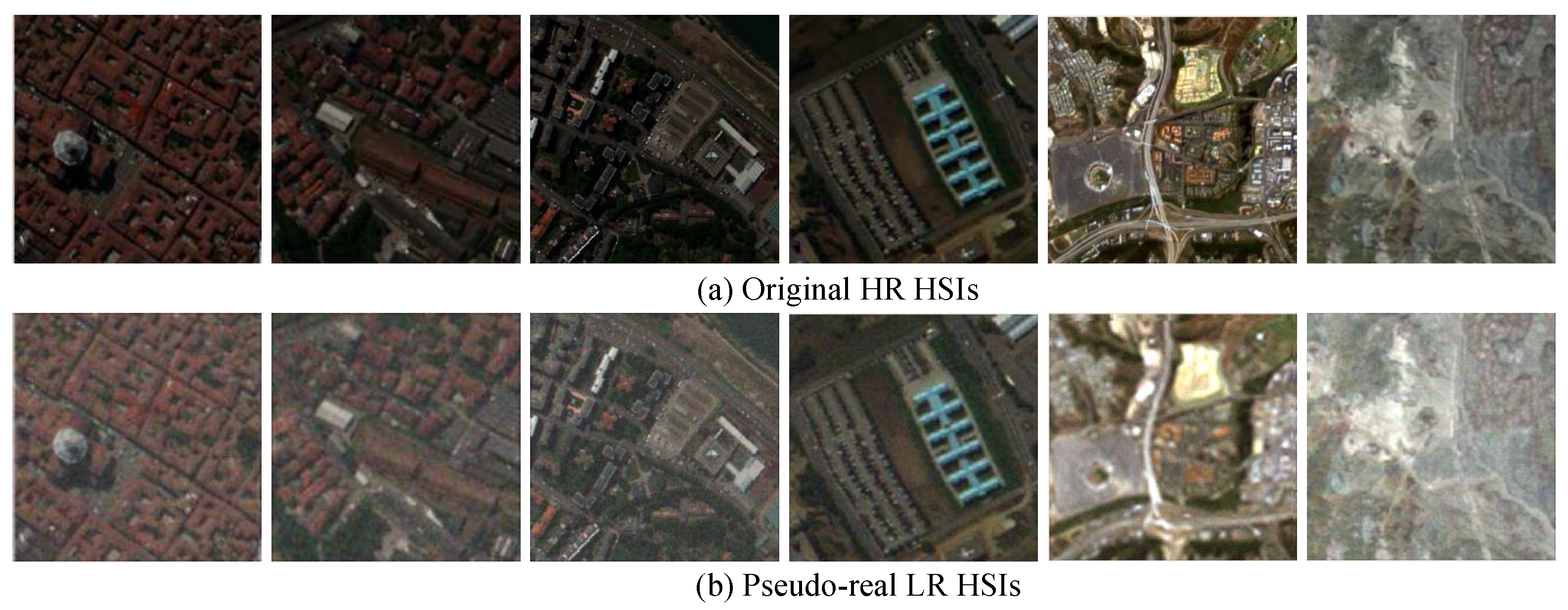
The pseudo-real data generated by the high-order degradation of the original HR HSI will serve as training samples for the proposed network. Some examples of the produced LR HSIs are displayed in Figure 2, indicating the diversity of unknown degradation models in HSI SR training sample construction.
3.3. Attention-Enhanced GAN
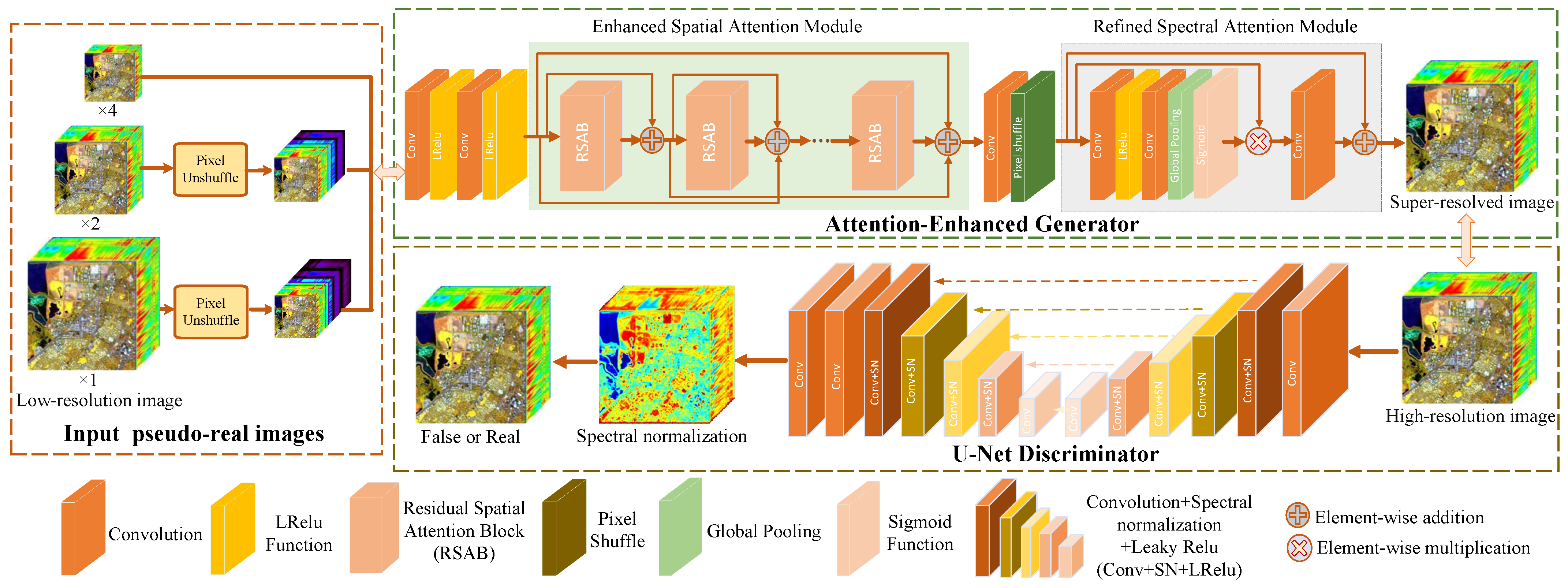
Currently, adversarial learning [14] is quite popular for coping with image-generation work, which has been utilized in the image SR task. In this work, a new attention-enhanced generative adversarial network (AEGAN) is specifically designed to improve the quality of HSI, as shown in Figure 3. In the proposed AEGAN, most of the computation is concentrated in a smaller resolution space, so that the consumption of GPU memory and other computing resources can be greatly reduced. Therefore, an inverse operation of pixel-shuffle [28], called pixel unshuffle, is firstly applied to the generated pseudo-real data, to increase its channel size and reduce its space size:
where and are the pseudo-real LR HSIs generated from original HR HSIs and the initial features obtained by pixel unshuffle operation , respectively.
The designed AEGAN consists of an attention-enhanced generator architecture with an ESAM and an RSAM, and a particular U-Net discriminator with spectral normalization. They are constructed to effectively capture more valuable and representative spatial-spectral characteristics and estimate the probability of an input HSI being real or false relative to the authentic HSI.
3.3.1. Attention-Enhanced Generator Architecture
With respect to HSI SR, the purpose of the generator architecture is to recover or generate the corresponding HR HSI with more authentic texture information derived from LR HSI. As depicted in Figure 3, according to the spatial-spectral characteristics of HSI, the attention-enhanced generator structure is designed with an ESAM and an RSAM to extract the spatial texture details and explore the spectral dependencies. The initial shallow features are extracted from the generated pseudo-real data through two convolutional layers with the convolution kernels of and , followed by the Leaky rectified linear unit (LReLU) activation function [52]:
in which represents the extracted shallow features, stands for the ReLU activation function, , and indicate the shallow feature extraction function of the first and the second convolutional layers, respectively.
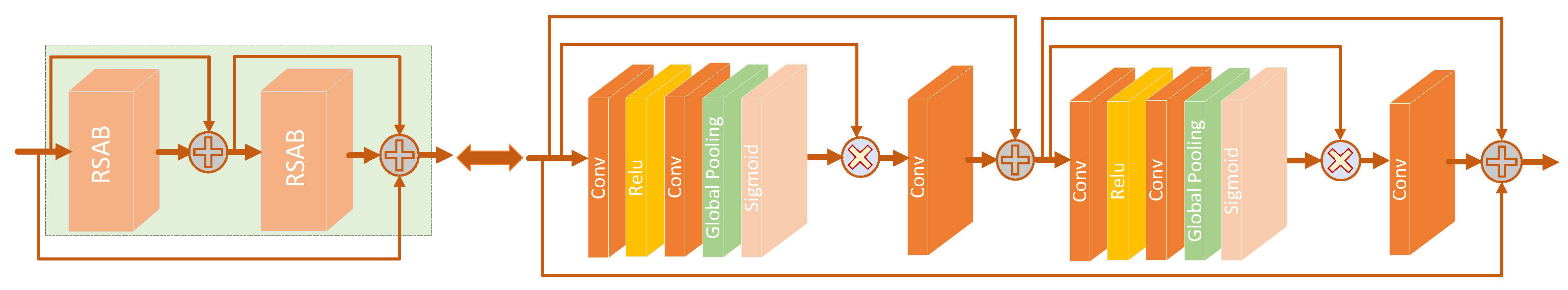
Next, the extracted shallow feature is transmitted into ESAM to further excavate and enhance more meaningful and informative characteristics. The designed ESAM with a dense connection aggregates the spatial attention mechanism into residual spatial attention blocks (RSABs) that can perform advanced feature extraction and comprises n cascading RSABs with an identical layout. The architecture of RSABs is displayed in Figure 4. A RSAB consists of CONV-ReLU-CONV with a kernel size of , a global pooling layer, a sigmoid layer, and a transition convolutional layer. Two RSABs are cascaded to explore the local and global spatial characteristics of HSIs. Accordingly, the output-enhanced spatial attention features can be formulated as follows:
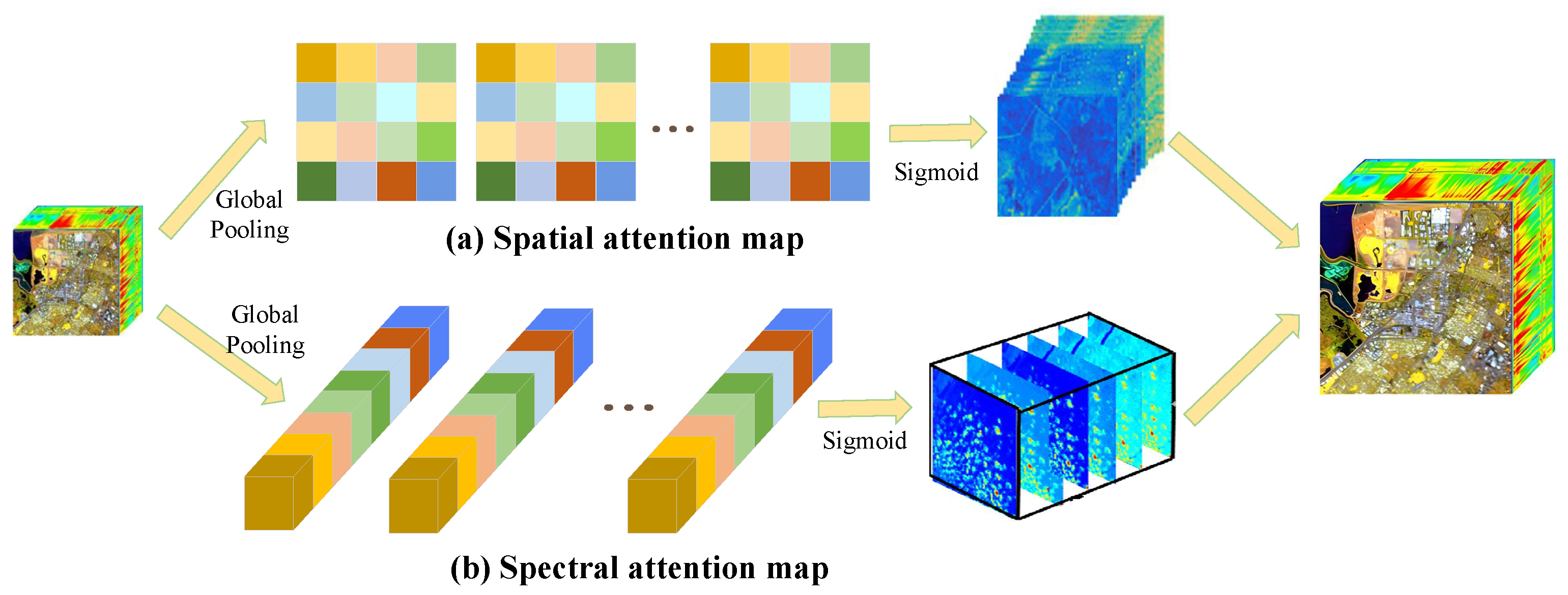
where and are the input of the n-th RSAB and the corresponding output of enhanced spatial attention features, respectively. and indicate the mapping function of RSAB and global pooling. represents the sigmoid activation function that maps the enhanced spatial features into the range of [0, 1], and ⊗ denotes the element-wise multiplication. Further, the spatial attention map is obtained (see Figure 5a), which emphasizes more informative spatial characteristics of HSI and suppresses useless features.
With their acquired enhanced spatial attention features, a convolutional layer and a sub-pixel convolution [28] layer are utilized to augment the spatial resolution of the input HSI to a desired size:
in which denotes the mapping function of upsampling layer and represents the feature maps after upsampling.
Analogously, to make full use of the spectral dependencies of HSI and reduce spectral distortion, an RSAM with spectral attention is also constructed to explore the spectral interrelationships and refine the holistic characteristics information of HSI. It is made up of CONV-ReLU-CONV with a kernel size of , a global pooling layer, a sigmoid layer, and a transition convolutional layer (as depicted in Figure 5b). The generated feature map using pseudo-real data can be represented as follows:
3.3.2. U-Net Discriminator with Spectral Normalization
In general GAN, the discriminator aims to simulate data distribution and learn the difference between the authentic image and the generated one through the penalizing generator to 0 or 1. It plays an indispensable role in the proposed method and directly affects the SR performance. Motivated by the work in [53], an U-Net structure with skip connections is employed as discriminator of the proposed network (the bottom part of Figure 3), to handle issues related to the spatial SR of HSI. The U-Net discriminator can not only furnish detailed pixel-by-pixel feedback to the attention-enhanced generator but also output the genuineness value of each pixel in HSI. Considering the possible instability in training caused by U-Net architecture and diverse degenerations, spectral normalization regularization [54] is introduced to the U-Net discriminator for training stabilization, oversharp, and artifacts mitigation.
In this paper, following [50,55], the U-Net discriminator with spectral normalization is composed of an encoder and a decoder, which are concatenated via skip connections. The encoder employs one convolutional layer with a stride of 1, and three convolutional layers with a kernel size of , each followed by a spectral normalization and a LReLU activation with a negative coeffient = 0.2. It is notable that, for the last two max-pooling layers, a stride of 2 is employed for downsampling to decrease the spatial size of HSI feature map and enlarge the receptive fields. To improve the representative capacity of the proposed network, the channel number is also increased accordingly. Similar to the conventional discriminator in [16], the relativistic discriminator estimates the holistic probability of an input HSI being actual or false relative to the authentic HSI. The loss function of an encoder can be formulated as
in which represents the ground-truth HR HSI, stands for the generated SR HSI, and means taking an average of all real or false HSIs. and denote the function of the relativistic discriminator and the output of the non-transformed discriminator, respectively.
The decoder increases the spatial resolution of the acquired feature map with the upsampling operator and propagates the context information to layers with a higher resolution. It contains three convolutional layers and two upsampling layers. Each convolutional layer is regularized with spectral normalization. To facilitate the information flow between low-level and high-level and promote the ability of discrimination, the output of encoder is concatenated with the input of decoder. Finally, two convolutional layers followed by LReLU and a convolutional layer with only one kernel followed by one sigmoid active function are employed to produce a binary mask (i.e., classification score) , which calculates the pixel-wise difference between the authentic and forged pixels of an input image. Accordingly, the loss function of decoder can be represented as
in which and denote the score maps of the ground-truth HR HSI and the generated SR HSI, respectively. That is, denotes the ground-truth HSI at pixel ; indicates the forged HSI at pixel ; and is opposite. Consequently, the total loss function for the U-Net discriminator can be represented as:
The size of final output feature of the U-Net discriminator is the same as that of the super-resolved HSI, indicating the similarity between corresponding pixels in the generated HSI and the realistic one. The closer the pixel similarity value is to 1, the closer the generated HSI is to the realistic HSI, and vice versa.
3.4. Attention-Enhanced Generative Loss
For HSI spatial SR, the selection of loss function is of considerable importance in optimizing the reconstruction performance of the GAN framework [56]. In this work, in order to achieve more realistic and detailed super-resolved HSI, an attention-enhanced generative loss function is devised to collectively train the proposed AEGAN and investigate the high correlation of spatial context and spectral information in HSI. It is composed of the pixel-wise-based spatial loss term , the perceptual loss term , the adversarial loss term , the attention loss term , and the spectral-angle-mapper based loss term and can be expressed as follows:
where , , , and denote the trade-off parameters to balance different loss terms, respectively. These hyperparameters determine the contribution of different loss terms in the attention-enhanced generative loss.
- Pixel-wise-based spatial loss term. With respect to the image SR, the mean-squared-error (MSE) is always employed as the loss of the neural network. Although the MSE-based loss function can gain higher peak signal-to-noise ratio (PSNR) and structural similarity index measurement (SSIM) values, there is still a large difference between the distribution of the super-resolved image and that of the actual one, such as edge smoothing, missing high-frequency details, etc. To make the restored HSI as close as possible to the actual HR HSI, the least absolute deviation (-norm) is adopted as a pixel-wise spatial loss term to restrict the content of the recovered HSI and guarantee the restoration accuracy of each pixel. Thereby, the least-absolute-deviation-based pixel-wise spatial loss term can be expressed as:where , , and L indicate the length, width, and spectral band number of , respectively. refers to the reconstructed HSI generated by pseudo-real data, and denotes the -norm.
- Perceptual-based loss term. Taking the particularity of HSI into consideration, the perceptual loss term is designed to make the reconstructed HSI perceptually approximate the actual HR HSI according to high-level characteristics obtained from a pre-trained deep network. Similar to [15,16], the recovered HSI and the ground-truth HR HSI are used together as the input of pre-training VGG19 to mine the features of VGG19-54 layer. The perceptual-based loss term can be defined asin which and denote the function of VGG and the generator, respectively.
- Adversarial-based loss term. The adversarial loss term represents the difference between the actual HR HSI and produced super-resolved HSI, which is committed to the self-optimization of generator with the return parameters of the discriminator and further facilitates more authentic HSI recovery. In this paper, the more powerful U-Net discriminator is applied to direct the attention-enhanced generator to lay emphasis on more valuable information, to improve restored textures and achieve better visual quality. Therefore, according to the loss function of discriminator, the corresponding adversarial loss for the attention-enhanced generator can be symmetrically expressed as:
It is notable that the higher the adversarial loss value is, the worse the reconstructed HSI is.
- Attention-based loss term. Although the adversarial loss of the attention-enhanced generator can deceive the discriminator by continuously updating the weights in the direction of generating sample distribution, it cannot guarantee accurate reconstruction for spectral information at the respective pixel positions. Inspired by [53], the classification score obtained by the U-Net discriminator is employed as the weighted attention loss of the attention-enhanced generator. This attention-based loss term is capable of evaluating the real or fake degree of each pixel position of HSI, leading to an attention-enhanced generator more focused on the parts of generated HSI that are difficult to produce and recover. The attention-based loss term can be defined asin which represents the classification score of the generated HSI derived by the U-Net discriminator.
- The SAM-based loss term. In order to constrain the spectral structure and reduce spectral distortion, the SAM loss is employed to predict the spectral similarity between the recovered spectrum and the authentic spectrum:where and stand for the spectral vector of the authentic HSI and the recovered image at the same spatial position , respectively. A smaller SAM value indicates that the two spectra are more similar.
The combination of the above loss terms with different weighting hyperparameters as shown in Equation (12) constrains the devised AEGAN model to produce more visually realistic results with fewer artifacts. The training procedure of the AEGAN model is thus summarized in Algorithm 1.
| Algorithm 1 Training procedure of our proposed method |
| Initialization: All network parameters are initialized [57] |
| Sample from pseud-real and authentic |
| are the batch size, iteration, and learning rate, respectively |
| for do |
| for n in N do |
| Calculate the loss function according to Equation (12) |
| update the parameters of attention-enhanced generator: |
| Calculate the loss function according to Equation (11) |
| update the parameters of U-Net discriminator: |
| end for |
| end for |
| save the attention-enhanced generative adversarial network. |
4. Experiments
In this section, numerous experiments are performed to evaluate the performance of the proposed AEGAN method. First, the experimental hyperspectral remote sensing datasets, implementation details, and quantitative evaluation criteria are introduced. Then, several relevant ablation studies, as well as comparative experiments with existing state-of-the-art, are conducted on both pseudo-real datasets and benchmark datasets.
4.1. Experimental Datasets and Implementation Details
In the experiment, three publicly available real datasets of hyperspectral remote sensing scenes (available online at http://www.ehu.eus/ccwintco/index.php/Hyperspectral_Remote_Sensing_Scenes, accessed on 9 January 2022) (Pavia University dataset, Pavia Center dataset and Cuprite dataset) are employed as original HSIs for validation. The Pavia University dataset covers 103 bands of the spectrum from 430 nm to 860 nm after discarding the noisy band and bad-band, containing 610 × 340 pixels in each spectral band with a geometric resolution of 1.3 m. The Pavia Center dataset collects 102 spectral bands after discarding bad-bands, comprising a total of 1096 × 1096 pixels in each spectral band. While in the Pavia Center scene, information on partial areas is not available, and only 1096 × 715 valid pixels remained in each spectral band. The cuprite dataset captures 202 valid spectral bands in the spectrum from 370 nm to 2480 nm after the corrupted bands’ removal, and each band consists of 512 × 614 pixels.
The input LR samples (the pseudo real data) are generated from original HSI samples by the high-order degeneration model with scaling factors of 2 and 4. The original HSI serves as the reference authentic image . For the employed three data sets, to testify to the effectiveness of the proposed AEGAN approach, some patches in size of 150 × 150 × L pixels with the richest texture details are cropped as testing images, and the remaining parts are utilized as training samples. To cope with the issue of inadequate training images, the training samples are augmented by flipping horizontally and rotating for , , . Therefore, the size of the LR HSI samples could be 36 × 36 × L or 72 × 72 × L, and the corresponding output HR HSIs are 144 × 144 × L.
The adaptive moment estimation (Adam) optimizer [58] with default exponential decay rates and is adopted for network training. All of the network training and testing is implemented on four NVIDIA GeForce GTX 1080Ti GPU adopting Pytorch (available online at https://pytorch.org, accessed on 9 January 2022) frameworks. Due to the constraint of GPU memory, following [55], the batch size is assigned to 16 and the initial learning rate is allocated to 0.0001, while the learning process is terminated in 2500 epochs. Coefficients of attention-enhanced generative loss function are empirically allocated as , , , and , respectively. Moreover, during training, to retain the spatial size of feature map after convolution, zero-padding operation is applied in all convolutional layers.
4.2. Evaluation Metrics
To comprehensively evaluate the performance of the developed HSI SR approach, several commonly used evaluation metrics are adopted, including the mean peak signal-to-noise ratio (MPSNR), the mean structural similarity index (MSSIM), the erreur relative global adimensionnelle de synthese (ERGAS), and the spectral angle mapper (SAM). MPSNR describes the similarity match based on the mean-square-error, and the MSSIM represents the structural consistency between the recovered HSI and the ground-truth one. In this work, both MPSNR and MSSIM are measured by the mean values in all spectral bands. ERGAS is a global image quality indicator measuring the band-wise normalized root of MSE between the super-resolved image and the authentic one. For spectral fidelity, and SAM investigates the spectral recovery quality by estimating the average angle between spectral vectors of the recovered HSI and the actual HSI. MPSNR close to and MSSIM close to 1, and SAM and ERGAS close to 0, denote a better reconstructed HR HSI.
Given a super-resolved HR HSI and an authentic HSI , the above-mentioned evaluation metrics can be respectively formulated as follows:
in which indicates the maximum intensity of the k-th band of HSI. , and , denote the average values and variances of and , respectively. stands for the covariance between and . and are two constants to improve stability, which are set to 0.01 and 0.03, respectively. stands for the dot product of two spectra vectors, denotes the -norm, and s represents the scaling factor.
4.3. Ablation Studies
In this work, ablation studies are conducted on the Pavia Center, Pavia University, and Cuprite datasets to illustrate the effectiveness of several specific designs in the proposed approach, including ESAM or RSAM in the attention-enhanced generator structure, the U-Net discriminator, the pseudo-real data generation, the pre-training and fine-tuning model, and the attention-enhanced generative loss function. The effectiveness of one component is testified and validated by removing it from the proposed method, while other components remain unchanged. Specifically, the baseline is set as employing bicubic downsampled HR HSI as LR HSI, replacing ESAM, RSAM, and the U-Net discriminator with ordinary convolutional layers.
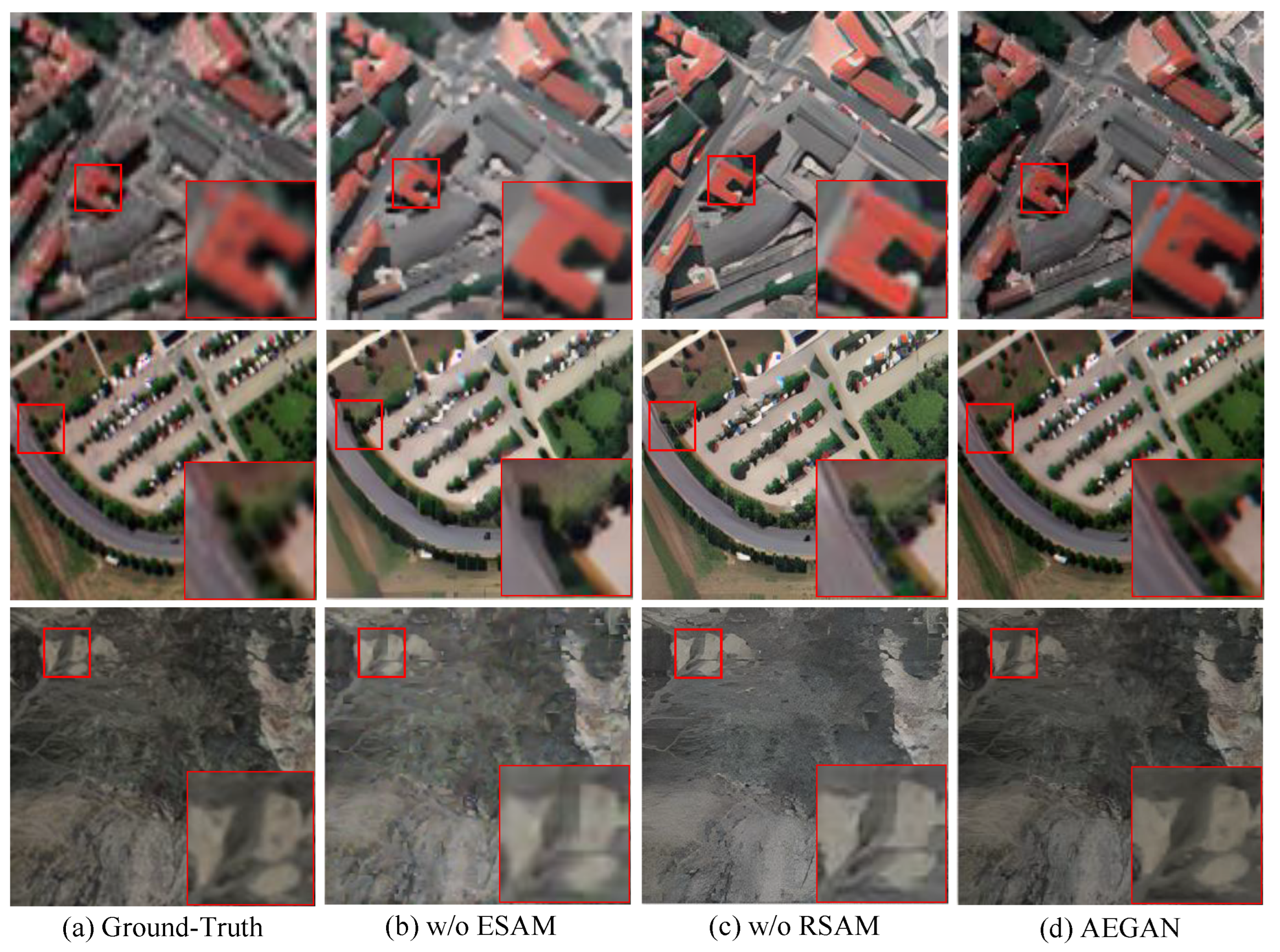
(1) Ablation study on ESAM or RSAM: To demonstrate the positive effect of ESAM and RSAM in the proposed method, ESAM or RSAM are removed from the attention-enhanced generator structure, denoted as w/o ESAM and w/o RSAM, respectively. It can be observed from Table 1 that both of them contribute to the performance improvement of the proposed approach. Particularly, without ESAM or RSAM in the attention-enhanced generator, the super-resolution performance severely deteriorates, i.e., MPSNR and MSSIM decrease by 0.3413dB and 0.0345, 0.1812dB and 0.0164, and 0.9498dB and 0.0553 on three HSI datasets, respectively. Moreover, the visual results of w/o ESAM and w/o RSAM are exhibited in Figure 6, as well as the reference ground truth. The result of w/o ESAM appears to be a little blurry, while the result of w/o RSAM seems too sharp, leading to a loss of detailed texture. The experimental results illustrate that ESAM is effective at improving and enhancing the feature representation ability of both low-frequency and high-frequency information, and RSAM is dedicated to finer texture detail reconstruction.
(2) Ablation study on U-Net discriminator: The U-Net discriminator (w/o U-Net) component is substituted with the simple convolutional layer. As shown in Table 1, it can be obviously seen that the performance of the proposed AEGAN approach is slightly better than that without the U-Net discriminator.
(3) Ablation study on Pseudo-real data generation: The pseudo-real data generation employs a high-order degradation model to better mimic the complicated authentic degradation procedure. To testify to its effectiveness, LR inputs obtained by bicubic interpolation are employed rather than the generated pseudo-real data (the corresponding method is denoted as w/o pseudo-real). From the results represented in Table 1, it can be observed with pseudo-real data generation that MPSNR and MSSIM are improved by 0.1397 dB and 0.0214, 0.1205 dB and 0.0095, and 0.0220 dB and 0.0217 for the three datasets, respectively.
(4) Ablation study on spatial attention and spectral attention: The core structures of ESAM and RSAM are the spatial attention block and spectral attention block in the residual connection of AEGAN. The influence of spatial attention and spectral attention of the proposed AEGAN model is also explored by removing spatial attention in ESAM (denoted as w/o SpaA) and removing spectral attention in RSAM (denoted as w/o SpeA), respectively. The corresponding experimental results on the Pavia Centre dataset at scale factor 4 are reported in Table 2. It can be observed that both spatial attention and spectral attention are conducive to improving the performance of ESAM and RSAM, in which MPSNR boosts 1.0282 dB and 1.1610 dB, MSSIM increases 0.0367 and 0.0439, SAM decreases 0.1474 and 0.1919, and ERGAS decreases 1.3486 and 1.4408 compared to the baseline model. Simultaneously, w/o ESAM differs from w/o SpaA with only 0.0015 in MPSNR, and w/o RSAM differs w/o SpeA with only 0.0032. Consequently, the construction and development of ESAM and RSAM in the proposed method exhibits a positive effect on the spatial-spectral characterization and improvement in HR HSI reconstruction.
(5) Ablation study on pre-training and fine-tuning: To demonstrate the effect of the pre-trained network model and fine-tuned network model, the pre-training and fine-tuning strategies are removed from the proposed network, respectively (denoted as w/o pre-training and w/o fine-tuning). The experimental results are tabulated in Table 3. It can be easily observed that the proposed AEGAN approach with the pre-training and fine-tuning strategies attains the superior results, avoiding the deterioration in both spatial and spectral evaluation. Concretely, with fine-tuning and pre-training strategies, the performance of the proposed AEGAN method is boosted by 0.7585 dB and 0.1874 dB in MPSNR and 0.0581 and 0.0294 in MSSIM, respectively. This reveals the fact that the pre-training and fine-tuning strategies are more beneficial for HSI SR and can remarkably improve the performance of the proposed approach.
(6) Ablation study on attention-enhanced generative loss function: To explore the effectiveness of different combination-based loss terms on the proposed network, ablation studies are carried out on the pixel-wise spatial-based loss term (), the perceptual-based loss term (), the adversarial-based loss term (), the attention-based loss term (), and the SAM-based loss term (). For HSI, the pixel-wise spatial-based loss term and SAM-based loss term can guarantee the fidelity and consistency of spatial-spectral structure information; therefore, the combination of and is regarded as the base in this paper. The quantitative experiment results using different combination-based loss terms on the Pavia Centre dataset at scale factor 4 are evaluated in Table 4. Clearly, combining the base with the adversarial-based loss function can promote the super-resolved performance of HSI by increasing 0.1457 dB and 0.0052 in MPSNR and MSSIM, respectively. The addition of perceptual loss term slightly improves the reconstruction performance of the network by boosting MPSNR with 0.0322 dB, making the reconstructed HSI perceptually approximate to the actual HR HSI. As shown in Table 4, coupled with attention-based loss term, the proposed method can acquire high-quality HR HSI estimation. This can be attributed to the accurate reconstruction of spectral information for each pixel and the finer expression of high-frequency spatial texture details spatially.
4.4. Comparison Experimental Results and Analysis
To illustrate the advancement of the proposed SR network, it is compared with different SR scenarios. The compared SR methods include the bicubic interpolation-based method [13], several representative CNN-based methods (SRCNN [26], 3D-FCNN [36], SSJSR [40], ERCSR [38], and HLNACNN [25]), and the GAN-based method (ESRGAN [16]).
Table 5 and Table 6 list the evaluation metrics of different SR approaches for the three benchmark hyperspectral datasets with a spatial upsampling factor of 2 and 4, respectively. It can be observed that the proposed AEGAN method outperforms all the other compared spatial SR approaches, producing SR results with the highest MPSNR and MSSIM and the lowest SAM and ERGAS. These demonstrate that the proposed AEGAN approach can well reconstruct the spatial texture and structural detail information of HSI.
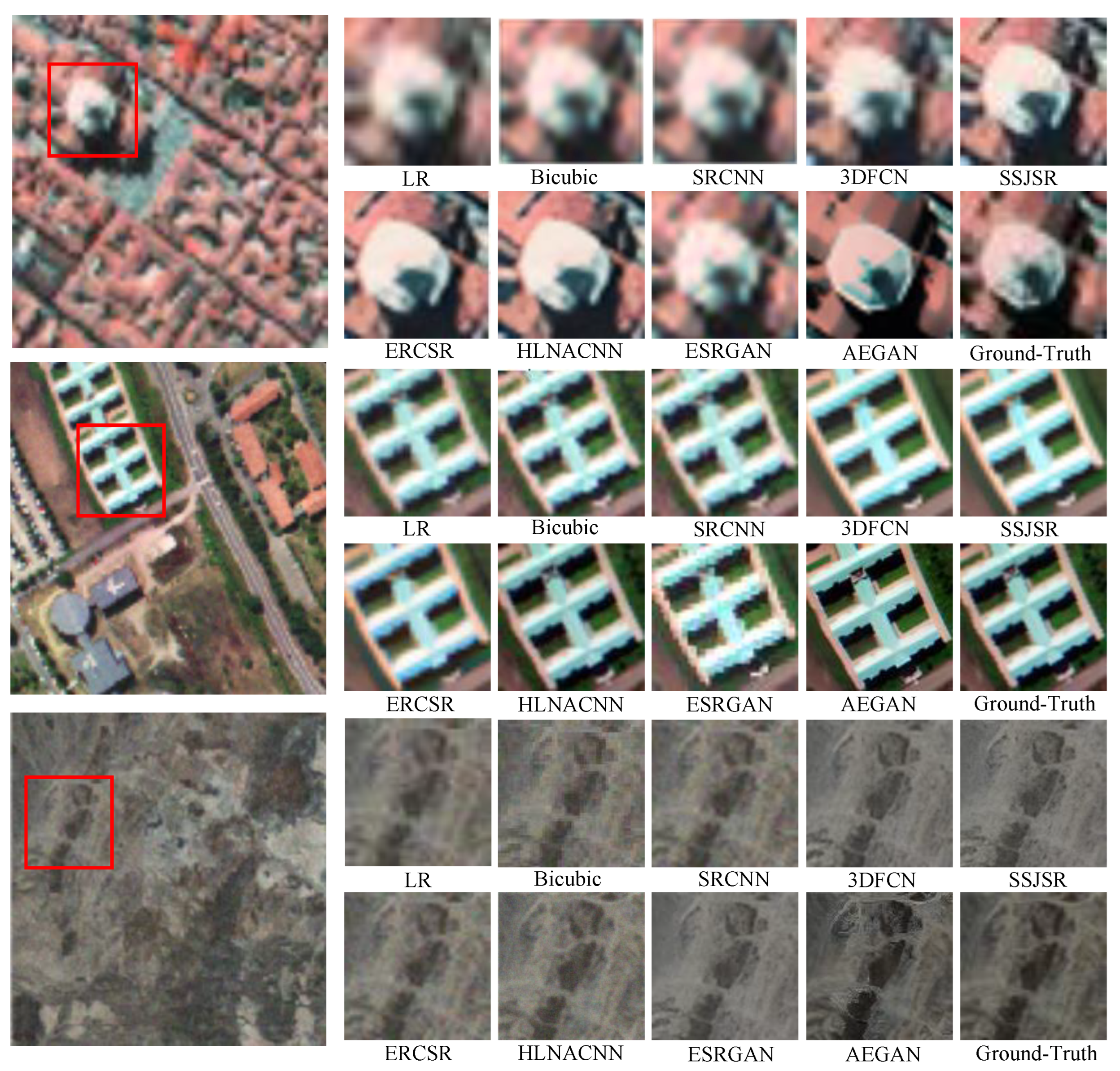
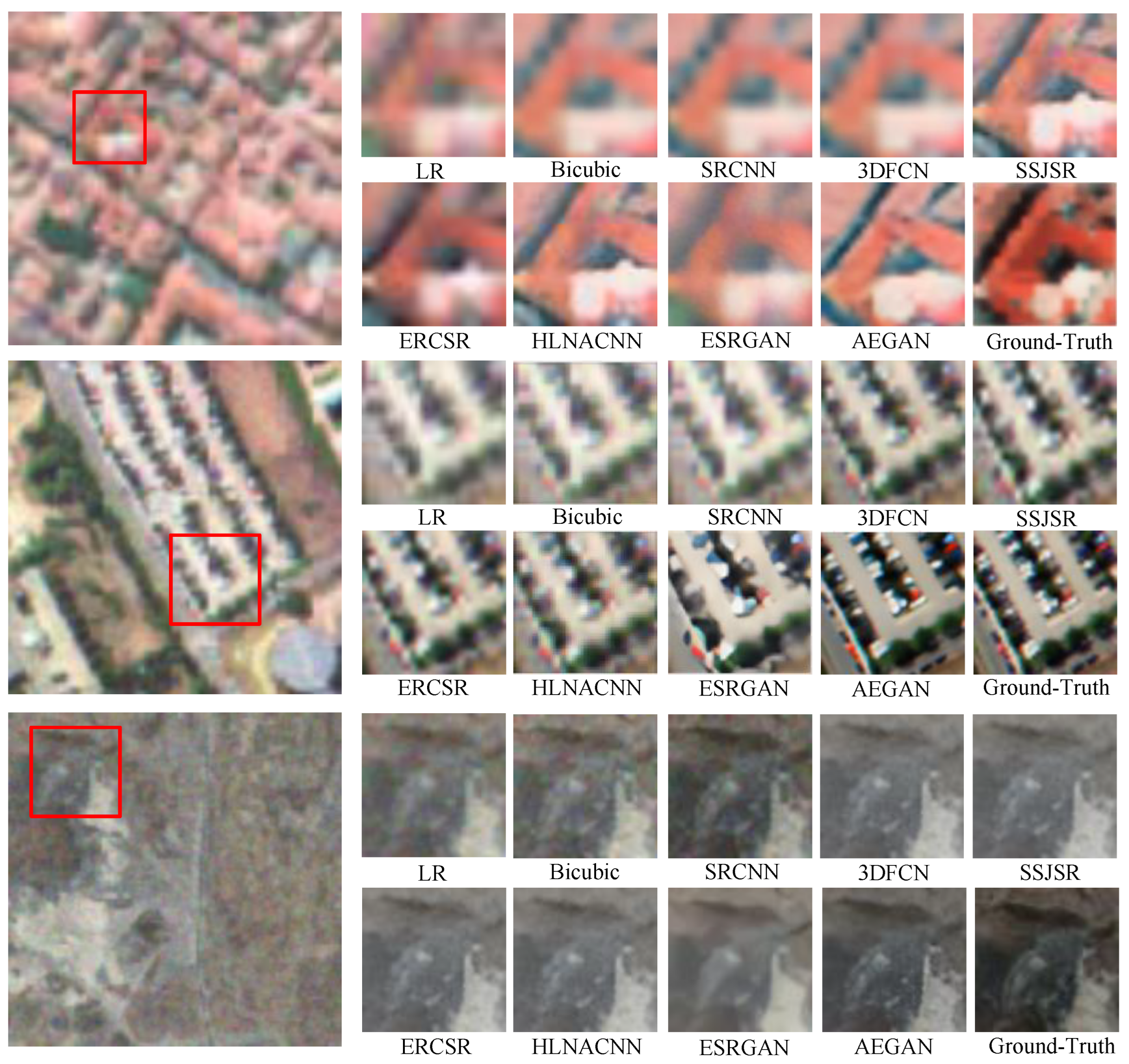
In order to better distinguish the reconstructed differences between the super-resolved HSI perceptually, parts of the super-resolved HSI generated by different methods are depicted in Figure 7 and Figure 8. It can be clearly observed that the proposed approach is capable of producing visually better HR HSI with finer textures and less blurring artifacts as well as distortion. Compared with the ground truth, the results generated by Bicubic, SRCNN, and 3DFCN suffer from severe blurring artifacts. SSJSR, ERCSR, and HLNACNN produce results lacking detailed information in some locations and introduce undesired noise. The results of ESRGAN are extreme and exhibit obvious distortion. By contrast, the proposed AEGAN approach can not only preserve the central structural information but also mitigate this distortion.
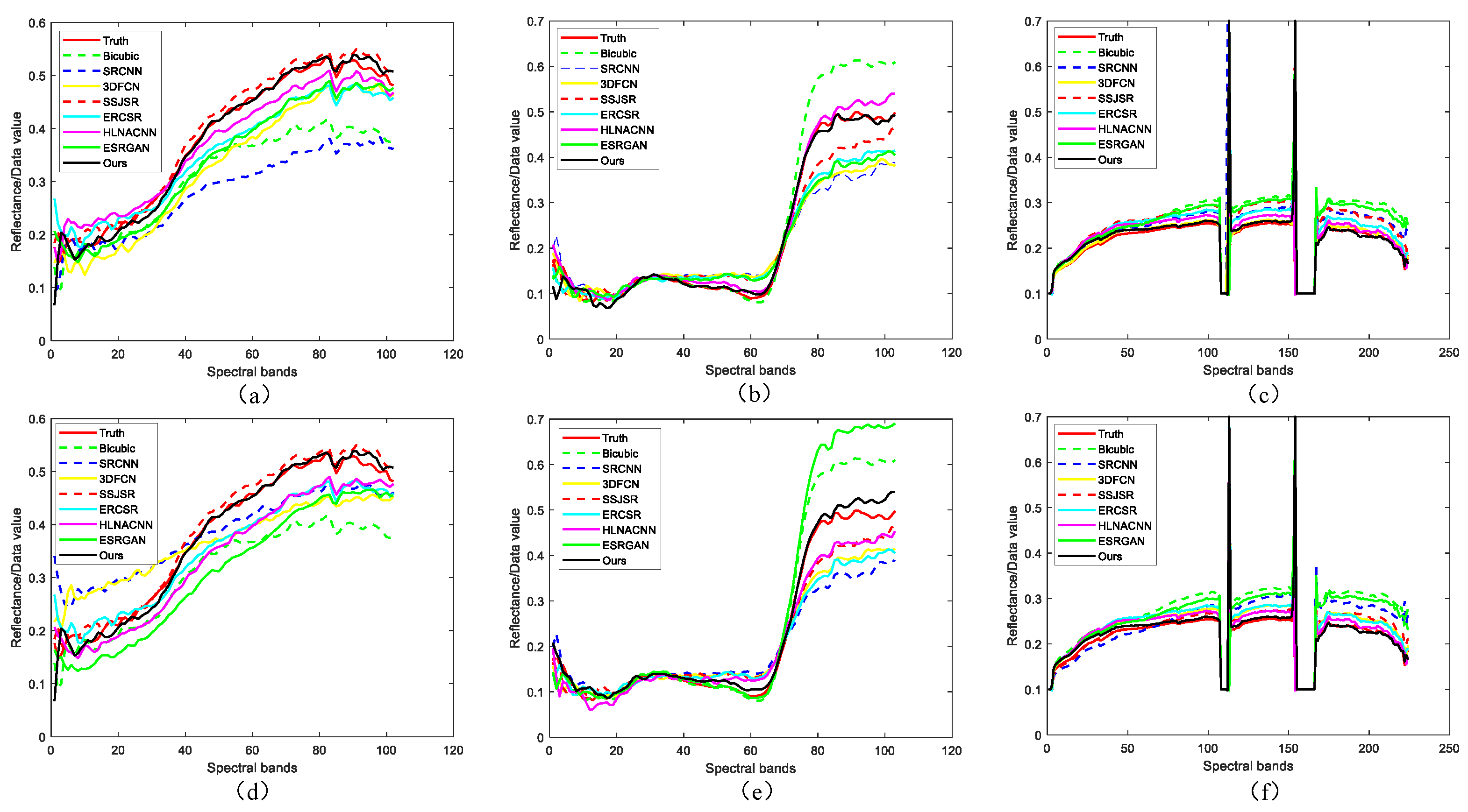
In addition, some reconstructed spectral curve graphs of different SR approaches are depicted in Figure 9. One pixel position is randomly selected for each dataset for spectral distortion analysis and discussion. It can be easily observed that all of the reconstructed spectral curves are consistent with the shape of ground-truth. In a few cases, the SRCNN approach and the ESRGAN approach have a certain degree of deviation, i.e., small spectral distortion, while the proposed AEGAN approach is the closest to the ground-truth, indicating its excellent performance in spectral information preservation.
We utilize the original codes of compared methods to calculate the parameter and complexity. Table 7 comprehensively shows the parameters, FLOPs, and inference time for different SR methods. We can see that our proposed method has the smallest computation burden.
5. Conclusions
In this paper, a new attention-enhanced generative adversarial network (AEGAN) for HSI spatial SR is proposed. The designed AEGAN contains an attention-enhanced generator architecture with an ESAM and an RSAM to effectively focus on and capture the more valuable and representative spatial-spectral characteristics of HSI. A special U-Net discriminator with spectral normalization is enclosed to stabilize the training and estimate the discriminative probability that the actual HR HSI is more similar to the fake generated image. Meanwhile, an attention-enhanced generative loss function is utilized to train the proposed model and investigate the high correlation of spatial context and spectral information, for the purpose of producing more realistic and detailed HSIs. Furthermore, to better simulate authentic degradation procedure, a high-order degradation model consisting of diverse degeneration estimation is also employed to produce the pseudo-real data for training. The experimental results on three benchmark HSI datasets illustrate its effectiveness and superiority in comparison with several existing state-of-the-art methods.
Although our proposed method exhibits advantages in hyperspectral image spatial super-resolution, it is still limited by the small number of data samples available for verifying network robustness. In future work, we plan to leverage the strengths of transformer models and integrate them into our network architecture to enhance its robustness and performance through extensive dataset training.
Author Contributions
Conceptualization, S.M.; methodology, B.W. and S.M.; validation, B.W. and S.M.; writing—original draft preparation, B.W., Y.Z. and S.M.; writing—review and editing, Y.F. and B.X.; supervision, B.W., Y.Z. and S.M.; and funding acquisition, S.M. All authors have read and agreed to the published version of the manuscript.
Funding
This research was supported by National Natural Science Foundation of China (No. 62171381).
Data Availability Statement
Publicly available datasets were analyzed in this study. This data can be found here: http://www.ehu.eus/ccwintco/index.php/Hyperspectral_Remote_Sensing_Scenes (accessed on 9 January 2021).
Conflicts of Interest
The authors declare no conflict of interest.
References
- Dian, R.; Li, S.; Kang, X. Regularizing hyperspectral and multispectral image fusion by CNN denoiser. IEEE Trans. Neural Netw. Learn. Syst. 2021, 32, 1124–1135. [Google Scholar] [CrossRef] [PubMed]
- Xie, W.; Shi, Y.; Li, Y.; Jia, X.; Lei, J. High-quality spectral-spatial reconstruction using saliency detection and deep feature enhancement. Pattern Recognit. 2019, 88, 139–152. [Google Scholar] [CrossRef]
- Cheng, G.; Lang, C.; Wu, M.; Xie, X.; Yao, X.; Han, J. Feature Enhancement Network for Object Detection in Optical Remote Sensing Images. J. Remote Sens. 2021, 1, 14. [Google Scholar] [CrossRef]
- Prasad, S.; Bruce, L.M. Limitations of Principal Components Analysis for Hyperspectral Target Recognition. IEEE Geosci. Remote Sens. Lett. 2008, 5, 625–629. [Google Scholar] [CrossRef]
- Zhang, L.; Zhang, L.; Tao, D.; Huang, X. A Multifeature Tensor for Remote-Sensing Target Recognition. IEEE Geosci. Remote Sens. Lett. 2011, 8, 374–378. [Google Scholar] [CrossRef]
- Xu, F.; Zhang, G.; Song, C.; Wang, H.; Mei, S. Multiscale and Cross-Level Attention Learning for Hyperspectral Image Classification. IEEE Trans. Geosci. Remote Sens. 2023, 61, 1–15. [Google Scholar] [CrossRef]
- Jia, S.; Zhan, Z.; Xu, M. Shearlet-Based Structure-Aware Filtering for Hyperspectral and LiDAR Data Classification. J. Remote Sens. 2021, 1, 25. [Google Scholar] [CrossRef]
- Mei, S.; Li, X.; Liu, X.; Cai, H.; Du, Q. Hyperspectral Image Classification Using Attention-Based Bidirectional Long Short-Term Memory Network. IEEE Trans. Geosci. Remote Sens. 2022, 60, 1–12. [Google Scholar] [CrossRef]
- Wang, B.; Zhang, S.; Feng, Y.; Mei, S.; Jia, S.; Du, Q. Hyperspectral Imagery Spatial Super-Resolution Using Generative Adversarial Network. IEEE Trans. Comput. Imaging 2021, 7, 948–960. [Google Scholar] [CrossRef]
- Li, J.; Cui, R.; Li, B.; Song, R.; Li, Y.; Dai, Y.; Du, Q. Hyperspectral Image Super-Resolution by Band Attention through Adversarial Learning. IEEE Trans. Geosci. Remote Sens. 2022, 58, 4304–4318. [Google Scholar] [CrossRef]
- Xu, Y.; Wu, Z.; Chanussot, J.; Wei, Z. Hyperspectral images super-resolution via learning high-order coupled tensor ring representation. IEEE Trans. Neural Netw. Learn. Syst. 2020, 31, 4747–4760. [Google Scholar] [CrossRef] [PubMed]
- Zhang, K.; Liang, J.; Van Gool, L.; Timofte, R. Designing a Practical Degradation Model for Deep Blind Image Super-Resolution. In Proceedings of the IEEE/CVF International Conference on Computer Vision (ICCV), Montreal, QC, Canada, 10–17 October 2021; pp. 4771–4780. [Google Scholar]
- Li, X.; Orchard, M.T. New edge-directed interpolation. IEEE Trans. Image Process. 2001, 10, 1521–1527. [Google Scholar] [PubMed] [Green Version]
- Goodfellow, I.J.; Pouget-Abadie, J.; Mirza, M.; Xu, B.; Warde-Farley, D.; Ozair, S.; Courville, A.; Bengio, Y. Generative Adversarial Networks. Adv. Neural Inf. Process. Syst. 2014, 3, 2672–2680. [Google Scholar] [CrossRef]
- Ledig, C.; Theis, L.; Huszár, F.; Caballero, J.; Aitken, A.P.; Tejani, A.; Totz, J.; Wang, Z.; Shi, W. Photo-realistic single image super-resolution using a generative adversarial network. In Proceedings of the IEEE Conference on Computer Vision and Pattern Recognition (CVPR), Honolulu, HI, USA, 21–26 July 2017; pp. 105–114. [Google Scholar]
- Wang, X.; Yu, K.; Wu, S.; Gu, J.; Tang, X. ESRGAN: Enhanced super-resolution generative adversarial networks. In Proceedings of the 15th European Conference on Computer Vision, Munich, Germany, 8–14 September 2018; pp. 63–79. [Google Scholar]
- Hu, J.; Shen, L.; Sun, G. Squeeze-and-excitation networks. In Proceedings of the IEEE Conference on Computer Vision and Pattern Recognition (CVPR), Salt Lake City, UT, USA, 18–22 June 2018; pp. 7132–7141. [Google Scholar]
- Woo, S.; Park, J.; Lee, J.-Y.; Kweon, I.S. CBAM: Convolutional block attention module. In Proceedings of the European Conference on Computer Vision (ECCV), GER, Munich, Germany, 8–14 September 2018; pp. 3–19. [Google Scholar]
- Irani, M.; Peleg, S. Improving resolution by image registration. Cvgip Graph. Model. Image Process. 1991, 53, 231–239. [Google Scholar] [CrossRef]
- Cao, Y.; Liu, X.; Wang, W.; Xing, Z. Super-resolution image reconstruction algorithm based on projection onto convex sets and wavelet fusion. J. Biomed. Eng. 2009, 26, 947–952. [Google Scholar]
- Schultz, R.R.; Stevenson, R.L. Improved definition image expansion. In Proceedings of the IEEE International Conference on Acoustics, Speech, and Signal Processing, San Francisco, CA, USA, 23–26 March 1992; pp. 173–176. [Google Scholar]
- Freeman, W.T.; Pasztor, E.C.; Carmichael, O.T. Learning low-level vision. Int. J. Comput. Vis. 2000, 40, 25–47. [Google Scholar] [CrossRef]
- Timofte, R.; De, V.; Gool, L.V. Anchored Neighborhood Regression for Fast Example-Based Super-Resolution. In Proceedings of the IEEE International Conference on Computer Vision, Sydney, NSW, Australia, 1–8 December 2013; pp. 1920–1927. [Google Scholar]
- Chang, H.; Yeung, D.Y.; Xiong, Y. Super-resolution through neighbor embedding. In Proceedings of the IEEE Computer Society Conference on Computer Vision and Pattern Recognition, Washington, DC, USA, 27 June–2 July 2004; pp. 275–282. [Google Scholar]
- Yang, J.; Xiao, L.; Zhao, Y.-Q.; Chan, J.C.-W. Hybrid Local and Nonlocal 3-D Attentive CNN for Hyperspectral Image Super-Resolution. IEEE Geosci. Remote Sens. Lett. 2021, 18, 1274–1278. [Google Scholar] [CrossRef]
- Dong, C.; Loy, C.C.; He, K.; Tang, X. Learning a deep convolutional network for image super-resolution. In Proceedings of the European Conference on Computer Vision, Zurich, Switzerland, 6–12 September 2014; Springer: Cham, Switzerland, 2014; pp. 184–199. [Google Scholar]
- Dong, C.; Loy, C.C.; Tang, X. Accelerating the super-resolution convolutional neural network. In Proceedings of the European Conference on Computer Vision, Amsterdam, The Netherlands, 11–14 October 2016; Springer: Cham, Switzerland, 2016; pp. 391–407. [Google Scholar]
- Shi, W.; Caballero, J.; Huszár, F.; Totz, J.; Aitken, A.P.; Bishop, R.; Rueckert, D.; Wang, Z. Real-time single image and video super-resolution using an efficient sub-pixel convolutional neural network. In Proceedings of the IEEE Conference on Computer Vision and Pattern Recognition, Las Vegas, NV, USA, 27–30 June 2016; pp. 1874–1883. [Google Scholar]
- Kim, J.; Lee, J.K.; Lee, K.M. Accurate image super-resolution using very deep convolutional networks. In Proceedings of the IEEE Conference on Computer Vision and Pattern Recognition (CVPR), Las Vegas, NV, USA, 27–30 June 2016; pp. 1646–1654. [Google Scholar]
- Lim, B.; Son, S.; Kim, H.; Nah, S.; Lee, K.M. Enhanced deep residual networks for single image super-resolution. In Proceedings of the IEEE Conference on Computer Vision and Pattern Recognition Work-Shops (CVPRW), Honolulu, HI, USA, 21–26 July 2017; pp. 1132–1140. [Google Scholar]
- He, K.; Zhang, X.; Ren, S.; Sun, J. Deep residual learning for image recognition. In Proceedings of the IEEE Conference on Computer Vision and Pattern Recognition (CVPR), Las Vegas, NV, USA, 27–30 June 2016; pp. 770–778. [Google Scholar]
- Tong, T.; Li, G.; Liu, X.; Gao, Q. Image super-resolution using dense skip connections. In Proceedings of the IEEE International Conference on Computer Vision (ICCV), Venice, Italy, 22–29 October 2017; pp. 4809–4817. [Google Scholar]
- Zhang, Y.; Tian, Y.; Kong, Y.; Zhong, B.; Fu, Y. Residual dense network for image super-resolution. In Proceedings of the IEEE Conference on Computer Vision and Pattern Recognition (CVPR), Salt Lake City, UT, USA, 18–22 June 2018; pp. 2472–2481. [Google Scholar]
- Yuan, Y.; Zheng, X.; Lu, X. Hyperspectral image super-resolution by transfer learning. IEEE J. Sel. Top. Appl. Earth Observ. Remote Sens. 2017, 10, 1963–1974. [Google Scholar] [CrossRef]
- Hu, J.; Li, Y.; Xie, W. Hyperspectral image super-resolution by spectral difference learning and spatial error correction. IEEE Geosci. Remote Sens. Lett. 2017, 14, 1825–1829. [Google Scholar] [CrossRef]
- Mei, S.; Yuan, X.; Ji, J.; Zhang, Y.; Wan, S.; Du, Q. Hyperspectral image spatial super-resolution via 3D full convolutional neural network. Remote Sens. 2017, 9, 1139. [Google Scholar] [CrossRef] [Green Version]
- Liu, D.; Li, J.; Yuan, Q. A spectral grouping and attention-driven residual dense network for hyperspectral image super-resolution. IEEE Trans. Geosci. Remote Sens. 2021, 59, 7711–7725. [Google Scholar] [CrossRef]
- Li, Q.; Wang, Q.; Li, X. Exploring the relationship between 2D/3D convolution for hyperspectral image super-resolution. IEEE Trans. Geosci. Remote. Sens. 2021, 59, 8693–8703. [Google Scholar] [CrossRef]
- Wang, X.; Ma, J.; Jiang, J. Hyperspectral image super-resolution via recurrent feedback embedding and spatial-spectral consistency regularization. IEEE Trans. Geosci. Remote. Sens. 2022, 60, 1–13. [Google Scholar] [CrossRef]
- Mei, S.; Jiang, R.; Li, X.; Du, Q. Spatial and Spectral Joint Super-Resolution Using Convolutional Neural Network. IEEE Trans. Geosci. Remote Sens. 2020, 99, 1–14. [Google Scholar] [CrossRef]
- Yang, J.; Zhao, Y.-Q.; Chan, J.C.-W.; Xiao, L. A multi-scale wavelet 3D-CNN for hyperspectral image super-resolution. Remote Sens. 2019, 11, 1557. [Google Scholar] [CrossRef] [Green Version]
- Jiang, J.; Sun, H.; Liu, X.; Ma, J. Learning Spatial-Spectral Prior for Super-Resolution of Hyperspectral Imagery. IEEE Trans. Comput. Imaging 2020, 6, 1082–1096. [Google Scholar] [CrossRef]
- Zhao, J.; Huang, T.; Zhou, Z. Hyperspectral image super-resolution using recursive densely convolutional neural network with spatial constraint strategy. Neural Comput. Appl. 2020, 32, 18. [Google Scholar] [CrossRef]
- Wang, Q.; Li, Q.; Li, X. Hyperspectral image super-resolution using spectrum and feature context. IEEE Trans. Ind. Electron. 2021, 68, 11276–11285. [Google Scholar] [CrossRef]
- Li, J.; Cui, R.; Li, Y.; Li, B.; Du, Q.; Ge, C. Multitemporal Hyperspectral Image Super-Resolution through 3D Generative Adversarial Network. In Proceedings of the 10th International Workshop on the Analysis of Multitemporal Remote Sensing Images (MultiTemp), Shanghai, China, 5–7 August 2019; pp. 1–4. [Google Scholar]
- Huang, Q.; Li, W.; Hu, T.; Tao, R. Hyperspectral Image Super-resolution Using Generative Adversarial Network and Residual Learning. In Proceedings of the IEEE International Conference on Acoustics, Speech and Signal Processing (ICASSP), Brighton, UK, 12–17 May 2019; pp. 3012–3016. [Google Scholar]
- Jiang, R.; Li, X.; Li, L.; Meng, H.; Yue, S.; Zhang, L. Learning Spectral and Spatial Features Based on Generative Adversarial Network for Hyperspectral Image Super-Resolution. In Proceedings of the IEEE International Geoscience and Remote Sensing Symposium, Yokohama, Japan, 28 July–2 August 2019; pp. 3161–3164. [Google Scholar]
- Liu, C.; Sun, D. On bayesian adaptive video super resolution. IEEE Trans. Pattern Anal. Mach. Intell. 2013, 36, 346–360. [Google Scholar] [CrossRef] [Green Version]
- Zhang, K.; Zhou, X.; Zhang, H.; Zuo, W. Revisiting single image super-resolution under internet environment: Blur kernels and reconstruction algorithms. In Proceedings of the Pacific Rim Conference on Multimedia, Gwangju, Republic of Korea, 16–18 September 2015; pp. 677–687. [Google Scholar]
- Wang, X.; Xie, L.; Dong, C.; Shan, Y. Real-ESRGAN: Training Real-World Blind Super-Resolution with Pure Synthetic Data. In Proceedings of the IEEE/CVF International Conference on Computer Vision Workshops (ICCVW), Montreal, BC, Canada, 11–17 October 2021; pp. 1905–1914. [Google Scholar]
- Liu, Y.; Du, X.; Shen, H.; Chen, S. Estimating generalized gaussian blur kernels for out-of-focus image deblurring. IEEE Trans. Circuits Syst. Video Technol. 2021, 31, 829–843. [Google Scholar] [CrossRef]
- Andrew, L.M.; Awni, Y.H.; Andrew, Y.N. Rectifier nonlinearities improve neural network acoustic models. In Proceedings of the International Conference Machine Learning, Atlanta, GA, USA, 16–21 June 2013; pp. 3–9. [Google Scholar]
- Schönfeld, E.; Schiele, B.; Khoreva, A. A U-Net Based Discriminator for Generative Adversarial Networks. In Proceedings of the IEEE/CVF Conference on Computer Vision and Pattern Recognition (CVPR), Seattle, WA, USA, 13–19 June 2020; pp. 8204–8213. [Google Scholar]
- Miyato, T.; Kataoka, T.; Koyama, M.; Yoshida, Y. Spectral normalization for generative adversarial networks. In Proceedings of the International Conference on Learning Representations (ICLR), Vancouver, BC, Canada, 30 April–3 May 2018. [Google Scholar]
- Yan, Y.; Liu, C.; Chen, C.; Sun, X.; Jin, L.; Zhou, X. Fine-Grained Attention and Feature-Sharing Generative Adversarial Networks for Single Image Super-Resolution. IEEE Trans. Multimed. 2022, 24, 1473–1487. [Google Scholar] [CrossRef]
- Qi, G.-J. Loss-sensitive generative adversarial networks on lipschitz densities. Int. J. Comput. Vis. (IJCV) 2017, 128, 1118–1140. [Google Scholar] [CrossRef] [Green Version]
- He, K.; Zhang, X.; Ren, S.; Sun, J. Delving Deep into Rectifiers: Surpassing Human-Level Performance on ImageNet Classification. In Proceedings of the IEEE International Conference on Computer Vision (ICCV), Santiago, Chile, 7–13 December 2015; pp. 1026–1034. [Google Scholar]
- Kingma, D.P.; Ba, J. Adam: A method for stochastic optimization. In Proceedings of the International Conference on Learning Representations, San Diego, CA, USA, 7–9 May 2015; pp. 1–15. [Google Scholar]
Figure 1.
The holistic framework of the proposed AEGAN method.

Figure 2.
Some examples of the LR HSIs generated by the high-order degradation model.

Figure 3.
The detailed architecture of attention-enhanced generator and U-Net discriminator.

Figure 4.
The architecture of the residual spatial attention block.

Figure 5.
The spatial attention map and the spectral attention map.

Figure 6.
The several visual results of the proposed approach with upsampling factor 2 for three hyperspectral image datasets. A red rectangular area is enlarged to display more clearly in reconstructed images. (a) the ground-truth, (b) the result of the proposed approach without ESAM, (c) the result of the proposed method without RSAM, and (d) the visual result of the AEGAN method.

Figure 7.
The visual results of super-resolved false-color comparisons of different SR methods with upsampling factor 2 for three hyperspectral image datasets (Pavia Center with spectral bands 65-30-25 as R-G-B channels, and Pavia University with spectral bands 55-30-15 as R-G-B channels and Cuprite with spectral bands 65-50-35 as R-G-B channels). Three demarcated areas (red frame) are zoomed for better visualization.

Figure 8.
The visual results of super-resolved false-color comparisons of different SR methods with upsampling factor 4 for three hyperspectral image datasets (Pavia Center with spectral bands 65-30-25 as R-G-B channels, Pavia University with spectral bands 55-30-15 as R-G-B channels, and Cuprite with spectral bands 65-50-35 as R-G-B channels). Three demarcated areas (red frame) are zoomed for better visualization.

Figure 9.
The recovered spectral curve graphs of different SR approaches with upsampling factor 2 (the top row) and 4 (the bottom row) for three hyperspectral image datasets. (a,d) the spectral curve graph at pixel position (360, 95) from Pavia Center dataset, (b,e) the spectral curve graph at pixel position (145, 85) from Pavia University dataset, and (c,f) the spectral curve graph at pixel position (190, 130) from Cuprite dataset.


Table 1.
Ablation investigations about different combinations of the pseudo-real data, ESAM or RSAM in generator, U-Net discriminator on Pavia Center, Pavia University, and Cuprite datasets, respectively, in which MPSNR, MSSIM, SAM, and ERGAS values over three HSI datasets are exhibited at scale factor 4.
| Model | Pavia Center | Pavia University | Cuprite | |||||||||
|---|---|---|---|---|---|---|---|---|---|---|---|---|
| MPSNR↑ | MSSIM↑ | SAM↓ | ERGAS↓ | MPSNR↑ | MSSIM↑ | SAM↓ | ERGAS↓ | MPSNR↑ | MSSIM↑ | SAM↓ | ERGAS↓ | |
| Baseline | 28.3193 | 0.7361 | 5.4927 | 7.9480 | 28.2258 | 0.7296 | 5.6180 | 8.0193 | 28.1752 | 0.8014 | 1.5931 | 7.4060 |
| w/o ESAM | 29.3490 | 0.7739 | 5.3490 | 6.5702 | 29.2803 | 0.7846 | 5.5901 | 7.3904 | 29.4018 | 0.8150 | 1.5700 | 6.3169 |
| w/o RSAM | 29.4835 | 0.7804 | 5.3015 | 6.4660 | 29.2951 | 0.7880 | 5.5784 | 7.1158 | 29.7064 | 0.8399 | 1.5587 | 6.0550 |
| w/o U-Net | 29.6360 | 0.7949 | 5.1803 | 6.4571 | 29.3790 | 0.7953 | 5.3759 | 6.9340 | 30.3350 | 0.8519 | 1.5380 | 5.5101 |
| w/o pseudo-real | 29.5506 | 0.7870 | 5.2164 | 6.4593 | 29.3410 | 0.7915 | 5.4020 | 7.0280 | 30.3296 | 0.8486 | 1.5401 | 5.5170 |
| AEGAN | 29.6903 | 0.8084 | 5.0217 | 6.4399 | 29.4615 | 0.8010 | 5.2823 | 6.6958 | 30.3516 | 0.8703 | 1.5245 | 5.5081 |
"↑: The higher MPSNR and MSSIM values denote better quality. ↓: The smaller SAM and ERGAS values denote better quality. The bold represent the best results.
Table 2.
The influence of spatial attention and spectral attention in the proposed approach on Pavia Centre dataset at scale factor 4.
Table 2.
The influence of spatial attention and spectral attention in the proposed approach on Pavia Centre dataset at scale factor 4.
| Evaluation Metrics | Baseline | w/o SpaA | w/o SpeA | AEGAN |
|---|---|---|---|---|
| MPSNR↑ | 28.3193 | 29.3475 | 29.4803 | 29.6903 |
| MSSIM↑ | 0.7361 | 0.7728 | 0.7800 | 0.8084 |
| SAM↓ | 5.4927 | 5.3453 | 5.3008 | 5.0217 |
| ERGAS↓ | 7.9480 | 6.5994 | 6.5072 | 6.4399 |
"↑: The higher MPSNR and MSSIM values denote better quality. ↓: The smaller SAM and ERGAS values denote better quality. The bold represent the best results.
Table 3.
The influence of pre-training and fine-tuning in the proposed network on Pavia Centre dataset at scale factor 4.
Table 3.
The influence of pre-training and fine-tuning in the proposed network on Pavia Centre dataset at scale factor 4.
| Evaluation Metrics | MPSNR↑ | MSSIM↑ | SAM↓ | ERGAS↓ |
|---|---|---|---|---|
| AEGAN (w/o pre-training) | 28.9318 | 0.7503 | 5.3962 | 7.3190 |
| AEGAN (w/o fine-tuning) | 29.5029 | 0.7790 | 5.1217 | 6.7035 |
"↑: The higher MPSNR and MSSIM values denote better quality. ↓: The smaller SAM and ERGAS values denote better quality.
Table 4.
Quantitative experiment results of different combination-based loss functions evaluated on the Pavia Centre dataset at the upsampling factor 4.
Table 4.
Quantitative experiment results of different combination-based loss functions evaluated on the Pavia Centre dataset at the upsampling factor 4.
| Losses | MPSNR↑ | MSSIM↑ | SAM↓ | ERGAS↓ |
|---|---|---|---|---|
| 29.5571 | 0.7899 | 5.0430 | 6.6407 | |
| 29.6028 | 0.7951 | 5.0394 | 6.5940 | |
| 29.6350 | 0.7990 | 5.0290 | 6.5105 | |
| 29.6903 | 0.8084 | 5.0217 | 6.4399 |
"↑: The higher MPSNR and MSSIM values denote better quality. ↓: The smaller SAM and ERGAS values denote better quality. The bold represent the best results.
Table 5.
Comparative results of different spatial SR methods for three different datasets are illustrated at the upsampling factor 2.
Table 5.
Comparative results of different spatial SR methods for three different datasets are illustrated at the upsampling factor 2.
| Method | Pavia Center | Pavia University | Cuprite | |||||||||
| MPSNR↑ | MSSIM↑ | SAM↓ | ERGAS↓ | MPSNR↑ | MSSIM↑ | SAM↓ | ERGAS↓ | MPSNR↑ | MSSIM↑ | SAM↓ | ERGAS↓ | |
| Bicubic | 31.8334 | 0.8762 | 4.1490 | 9.2563 | 31.5931 | 0.8650 | 4.2271 | 9.2834 | 33.3023 | 0.9188 | 1.2965 | 7.2471 |
| SRCNN [26] | 33.4803 | 0.9171 | 4.0370 | 7.1481 | 32.1961 | 0.9134 | 4.0119 | 7.2306 | 34.3151 | 0.9377 | 1.3075 | 6.4908 |
| 3DFCN [36] | 33.8109 | 0.9220 | 3.9908 | 6.9812 | 33.0397 | 0.9275 | 3.9974 | 6.9948 | 35.1075 | 0.9426 | 1.4437 | 5.8919 |
| SSJSR [40] | 34.6586 | 0.9405 | 4.3007 | 6.0348 | 33.7449 | 0.9392 | 3.8712 | 6.2589 | 33.9138 | 0.9532 | 1.8979 | 6.8116 |
| ERCSR [38] | 34.3492 | 0.9346 | 4.3841 | 6.5912 | 33.5091 | 0.9324 | 4.4627 | 6.3091 | 34.5042 | 0.9583 | 1.2896 | 6.2735 |
| HLNACNN [25] | 34.5916 | 0.9372 | 4.0158 | 6.2420 | 34.3278 | 0.9506 | 3.7057 | 6.0523 | 35.0258 | 0.9607 | 1.2841 | 6.0167 |
| ESRGAN [16] | 33.8358 | 0.9219 | 4.6385 | 6.9677 | 33.2963 | 0.9208 | 4.7425 | 6.9714 | 33.7046 | 0.9280 | 1.6013 | 7.0126 |
| AEGAN | 35.7450 | 0.9737 | 3.5860 | 5.2038 | 34.9816 | 0.9691 | 3.7029 | 5.6334 | 35.9002 | 0.9811 | 0.5497 | 5.0541 |
"↑: The higher MPSNR and MSSIM values denote better quality. ↓: The smaller SAM and ERGAS values denote better quality. The bold represent the best results.
Table 6.
Comparative results of different spatial SR methods for three benchmark hyperspectral datasets are illustrated at scale factor 4.
Table 6.
Comparative results of different spatial SR methods for three benchmark hyperspectral datasets are illustrated at scale factor 4.
| Method | Pavia Center | Pavia University | Cuprite | |||||||||
| MPSNR↑ | MSSIM↑ | SAM↓ | ERGAS↓ | MPSNR↑ | MSSIM↑ | SAM↓ | ERGAS↓ | MPSNR↑ | MSSIM↑ | SAM↓ | ERGAS↓ | |
| Bicubic | 28.1904 | 0.6979 | 5.2924 | 8.1943 | 28.0682 | 0.6775 | 5.9026 | 8.2901 | 27.5175 | 0.7588 | 1.8079 | 7.9346 |
| SRCNN [26] | 28.4791 | 0.7405 | 5.4873 | 8.0132 | 28.1932 | 0.7327 | 5.6707 | 8.1009 | 27.9950 | 0.7926 | 1.6017 | 7.5185 |
| 3DFCN [36] | 28.6176 | 0.7438 | 5.3806 | 7.8418 | 28.5122 | 0.7245 | 5.6144 | 7.9053 | 28.8556 | 0.8169 | 1.7338 | 7.0156 |
| SSJSR [40] | 29.0535 | 0.7747 | 5.2925 | 7.0927 | 29.0071 | 0.7790 | 5.5528 | 7.1054 | 28.7237 | 0.8247 | 1.9408 | 7.1918 |
| ERCSR [38] | 29.0302 | 0.7590 | 5.3915 | 7.3180 | 28.9518 | 0.7527 | 5.6446 | 7.9175 | 28.9061 | 0.8279 | 1.7174 | 7.0083 |
| HLNACNN [25] | 29.0469 | 0.7633 | 5.2641 | 7.1945 | 28.9933 | 0.7605 | 5.5915 | 7.3039 | 28.9810 | 0.8365 | 1.7090 | 6.8427 |
| ESRGAN [16] | 28.1514 | 0.7329 | 7.7107 | 8.2090 | 28.0365 | 0.7218 | 7.9254 | 8.2850 | 27.6203 | 0.7782 | 3.3764 | 7.8140 |
| AEGAN | 29.6903 | 0.8084 | 5.0217 | 6.4399 | 29.4615 | 0.8010 | 5.2823 | 6.6958 | 30.3516 | 0.8703 | 1.5245 | 5.5081 |
"↑: The higher MPSNR and MSSIM values denote better quality. ↓: The smaller SAM and ERGAS values denote better quality. The bold represent the best results.
Table 7.
The parameter and computation comparison with different SR models at scale factor 4.
| Model | SRCNN | 3DFCN | SSJSR | ERCSR | HLNACNN | ESRGAN | AEGAN |
|---|---|---|---|---|---|---|---|
| Params | 16.3 M | 21.7 M | 20.1 M | 17 M | 18.6 M | 15.4 M | 11.6 M |
| FLOPs | 215.7 G | 273.5 G | 244.1 G | 182.5 G | 202.3 G | 148.2 G | 109.7 G |
| Inference time | 0.585 s | 0.973 s | 0.814 s | 0.703 s | 0.752 s | 0.696 s | 0.731 s |
Disclaimer/Publisher’s Note: The statements, opinions and data contained in all publications are solely those of the individual author(s) and contributor(s) and not of MDPI and/or the editor(s). MDPI and/or the editor(s) disclaim responsibility for any injury to people or property resulting from any ideas, methods, instructions or products referred to in the content. |
© 2023 by the authors. Licensee MDPI, Basel, Switzerland. This article is an open access article distributed under the terms and conditions of the Creative Commons Attribution (CC BY) license (https://creativecommons.org/licenses/by/4.0/).
Share and Cite
MDPI and ACS Style
Wang, B.; Zhang, Y.; Feng, Y.; Xie, B.; Mei, S. Attention-Enhanced Generative Adversarial Network for Hyperspectral Imagery Spatial Super-Resolution. Remote Sens. 2023, 15, 3644. https://0-doi-org.brum.beds.ac.uk/10.3390/rs15143644
AMA Style
Wang B, Zhang Y, Feng Y, Xie B, Mei S. Attention-Enhanced Generative Adversarial Network for Hyperspectral Imagery Spatial Super-Resolution. Remote Sensing. 2023; 15(14):3644. https://0-doi-org.brum.beds.ac.uk/10.3390/rs15143644
Chicago/Turabian StyleWang, Baorui, Yifan Zhang, Yan Feng, Bobo Xie, and Shaohui Mei. 2023. "Attention-Enhanced Generative Adversarial Network for Hyperspectral Imagery Spatial Super-Resolution" Remote Sensing 15, no. 14: 3644. https://0-doi-org.brum.beds.ac.uk/10.3390/rs15143644
Note that from the first issue of 2016, this journal uses article numbers instead of page numbers. See further details here.