
Sea Surface Roughness Determination from Grazing Angle GPS Ocean Observations and Scatterometry Simulations

1
Department of Physics, University of Oslo, 0316 Oslo, Norway
2
Beyond Gravity Sweden, 415 05 Gothenburg, Sweden
*
Author to whom correspondence should be addressed.
Remote Sens. 2023, 15(15), 3794; https://0-doi-org.brum.beds.ac.uk/10.3390/rs15153794
Submission received: 31 May 2023
/
Revised: 11 July 2023
/
Accepted: 20 July 2023
/
Published: 30 July 2023
(This article belongs to the Special Issue Radio Occultation Climate Data Records and Application)
Abstract
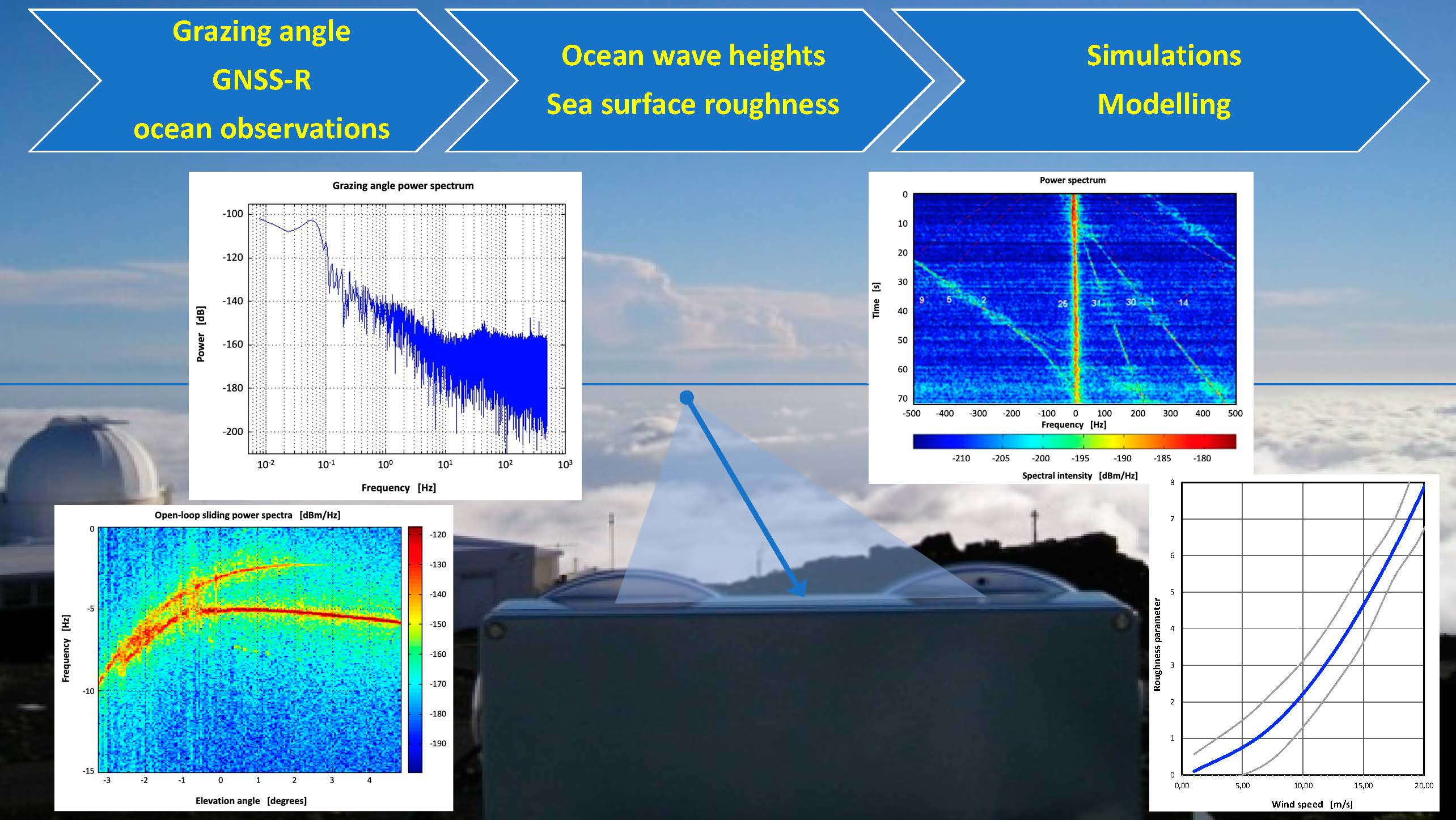
:Measurements of grazing angle GNSS-R ocean reflections combined with meteorological troposphere data are used for retrieval of ocean wave heights and surface roughness parameters. The observational results are compared to multiphase screen simulations for the same atmosphere conditions. The retrieved data from observations and simulations give equal results within the error bounds of the methods. The obtained ocean mean wave-heights are almost proportional to the square of the wind speed when applying a first-order approximation model to the high-wave-number part of the measured GNSS-R power spectra. The spectral variances from the measurements link directly to the ocean surface roughness, which is also verified by the performed multiple phase-screen wave propagation simulations. Thus, grazing angle GNSS-R techniques are an efficient method for determining the ocean state and the conditions in the boundary layer of the troposphere.

1. Introduction
The use of signals from the GNSS satellites in scatterometry constitutes a relatively new scientific area. Determination of parameters such as sea surface roughness, winds, ocean wave-heights, spectra, and tilts can be extracted from a spectral analysis of sea surface GNSS reflection measurements.
A number of measurement campaigns from mountain tops, airplanes, and satellites have shown results leading to some of these parameters [1,2,3]. International satellite missions, such as TDS-1, CYGNSS, COSMIC-2, the European satellite project proposals GEROS and G-TERN, and the ESA Scout mission proposal HydroGNSS, have underlined the need for simulation studies highlighting the assumptions for the data retrievals and the precision and the accuracy of such measurements [4,5,6,7,8,9,10,11].
Ocean reflected signals from the GNSS satellites (received at low Earth orbiting satellites, airplanes, and fixed mountain locations) describe the ocean surface mean height, waves, and sea surface roughness. The estimated accuracy of the average surface height is on the order of 10 cm for smooth and stable conditions. Thus, global observations could be an important contribution to long-term variations of the ocean mean height, as well as the monitoring of ocean mesoscale eddies (with spatial features of 100 km and temporal variability of the order of several days), which result in sea height changes much larger than the accuracy of the GNSS technique.
The ocean reflected signals can be divided into two set of measurements, (1) high-elevation measurements (equal to low incidence angles) and (2) low-elevation grazing angle measurements. For the first type, the ocean reflection cross-section has a limited extent. The reflected signal is coherent with smaller errors due to ocean waves, sampling rate, and the internal processing method of the receiver [6,11,12]. For low elevations, the signal reveals the incoherent scatter process in the reflection zone. Using open-loop high-precision GNSS receivers, it is possible to provide the in-phase I and quadrature Q components of the signal at high sample rates, which enables investigation of the spectral signatures of the received reflected GNSS signals.
The reflected signal is able to establish experimental knowledge on the influence of signal multipath interference and signal disturbances caused by the atmosphere and the ocean reflection. To quantify the potential, we performed a series of high-altitude ocean reflection measurements from the Haleakala Summit on Maui, Hawaii in 2004, revealing the spectral characteristics of the direct satellite signal and the ocean reflected signal for grazing elevation angles.
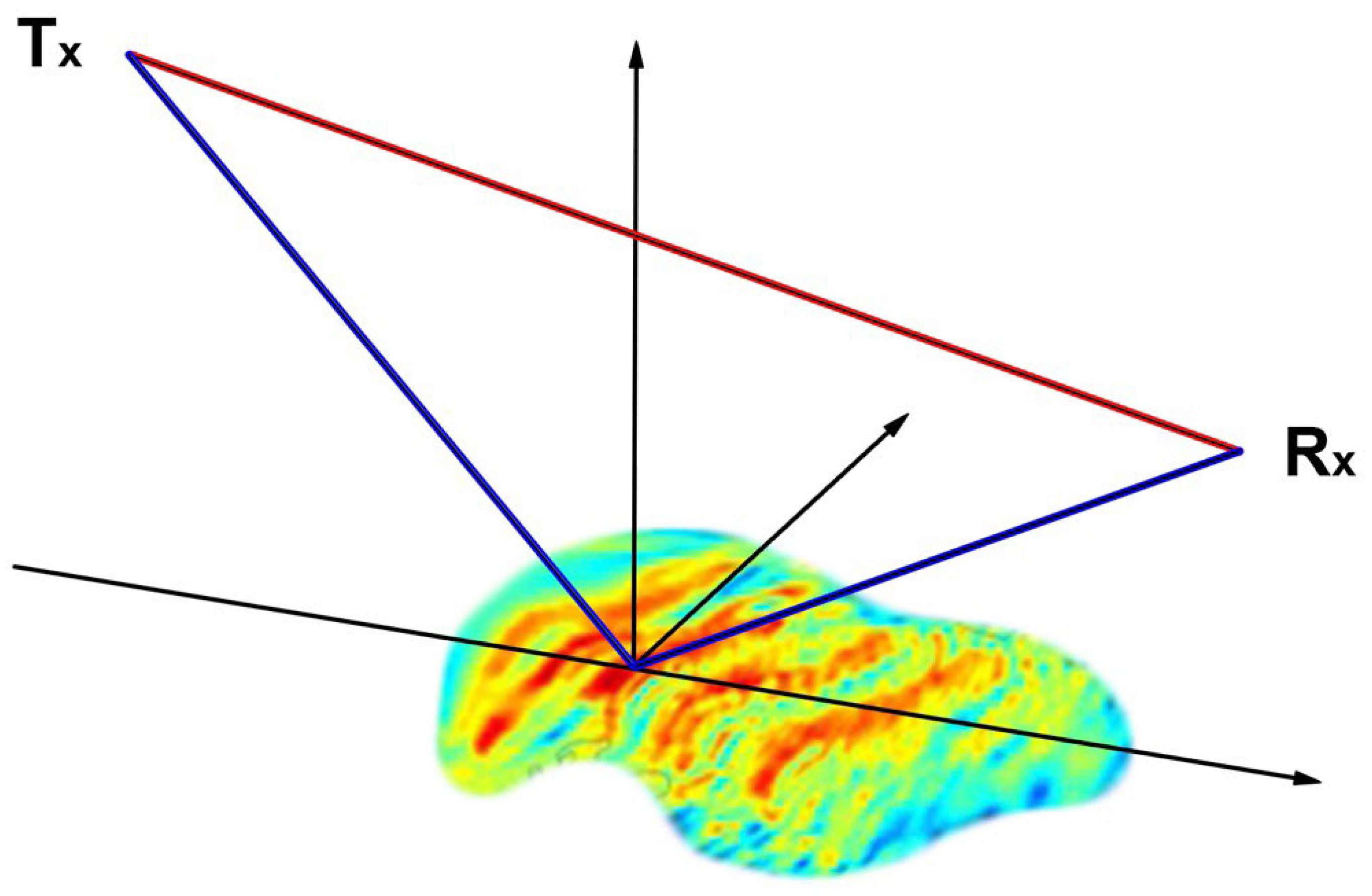
The experimental setup was a bistatic scattering system, consisting of a GPS satellite emitting electromagnetic waves, which are reflected by the ocean surface, and a GPS receiver at a low elevation angle. Both the direct wave and the reflected wave are collected by the receiver, as depicted in Figure 1.
The color-coded ocean surface heights in Figure 1 originate a retrieval of ocean and atmosphere conditions from a numerical weather prediction model (NWP). Large positive heights are colored red. While blue heights have lower surface altitudes compared to a mean ocean surface model for the area. Bands of higher wave heights are easy to identify with rather long scale sizes in the vertical plane containing Tx and Rx. Due to the resolution in the NWP calculation shorter wave lengths are smeared out in the plot. The bands of positive wave heights extend almost perpendicular to the plane containing the surface reflection observations, which could indicate a uniform atmosphere wind field in the region.
The characteristics of the reflected signal depend on the scattering properties of the sea surface and the footprint of the reflection zone. The footprint size and shape in turn depend on the geometry of the measurements and the relative velocities of transmitter and receiver with respect to the reflection zone. Thus, the characteristics of the scattering properties depend on several conditions for determining the roughness of the ocean.
The paper describes a wave propagator that can be used to simulate GNSS reflected signals from ocean surfaces. The wave propagator simulates the characteristics of a bi-static scattering system, where the transmitted wave from a GNSS satellite is detected by a GNSS receiver after the wave has been reflected by the ocean surface.
The theory of propagation of microwaves in the atmosphere is well established, and methods for the propagation range from ray tracing to numerical solutions to the wave equation. In addition to ray tracing, there are propagation methods that use mode theory [13] and a finite difference solution to the parabolic equation [14,15]. The presented propagator in this paper is based on the solution of the parabolic equation. The parabolic equation is solved using the split-step sine transformation. The Earth’s ocean surface is modeled using an impedance model. The concept gives an accurate lower boundary condition in the determination of the electromagnetic field and makes it possible to simulate reflections and the effects of transitions between different media [16].
This paper is divided into six separate sections: Section 1 introduces the GNSS-R measurement technique and the experimental setup for the observations; Section 2 explains the observations and the GNSS-R instrument used for obtaining the data; Section 3 describes the retrieval of ocean wave heights and sea surface roughness parameters from the measurements; Section 4 gives a description of the theory needed to perform the simulations of the bistatic scattering system and the retrieved estimates of wave heights and surface roughness, followed by a discussion in Section 5; Section 6 forms the conclusions.
2. Methods and Observations
High-altitude GPS measurements made at the Haleakala Summit on Maui, Hawaii, have revealed the spectral characteristics of the direct signal and the ocean reflected signal. The altitude of the observation site at 3040 m gave a long line-of-sight view over the ocean to the horizon with multiple paths primarily due to the ocean surface roughness. The chosen high altitude gives a signal only impacted by the ocean wave structures in the reflection zone at several hundred kilometers from the coast.
The receiving part of the instrument comprises separate L1 and L2 antennas both oriented with the main gain lobe toward the horizon. The two receiving antennas were directionally centered on the horizon toward south-southwest having an antenna opening angle of 50°. In this way, all ocean reflected measurements only sensed multiple paths due to ocean reflections since no other obstacles were in the field of view of the antennas. The use of directive antennas pointed toward the horizon enabled signal recordings down to the lowest layers of the atmosphere.
The instrumentation consisted of a prototype high-precision GNSS receiver, equivalent to the GNSS receiver flying on the EUMETSAT MetOp satellites, linked to an ultra-stable atomic clock [17,18]. The rubidium reference oscillator gave an improved temporal stability with an Allen deviation of 2 × 10⁻¹². This way timing errors were minimized to only the thermal noise of the instrument.
One of the key features of the instrument is the open-loop tracking mode. Since carrier tracking is not reliable, when turbulent conditions drive the measurements, code phase measurements are chosen to capture the signal at a prescribed frequency, named the Doppler model [17,19]. The open-loop tracking mode combined with high sampling rates of 100–1000 Hz identifies the navigation and atmosphere modulation, clock frequency errors, and errors caused by the Doppler model. It turns out that the Doppler model is independent of atmosphere conditions and the position of the observations on Earth (independent of polar, mid-latitudinal, and equatorial conditions) [17]. However, the Doppler model is a function of the straight-line tangent altitude between the GNSS satellite and the receiver, which in the spectral domain defines the center of the power spectrum. The lowest altitude between this straight-line and the ocean defines the straight-line tangent altitude for the applied time window used in the spectral analysis. The straight-line tangent altitude can be down to −35 km during grazing angle measurements.
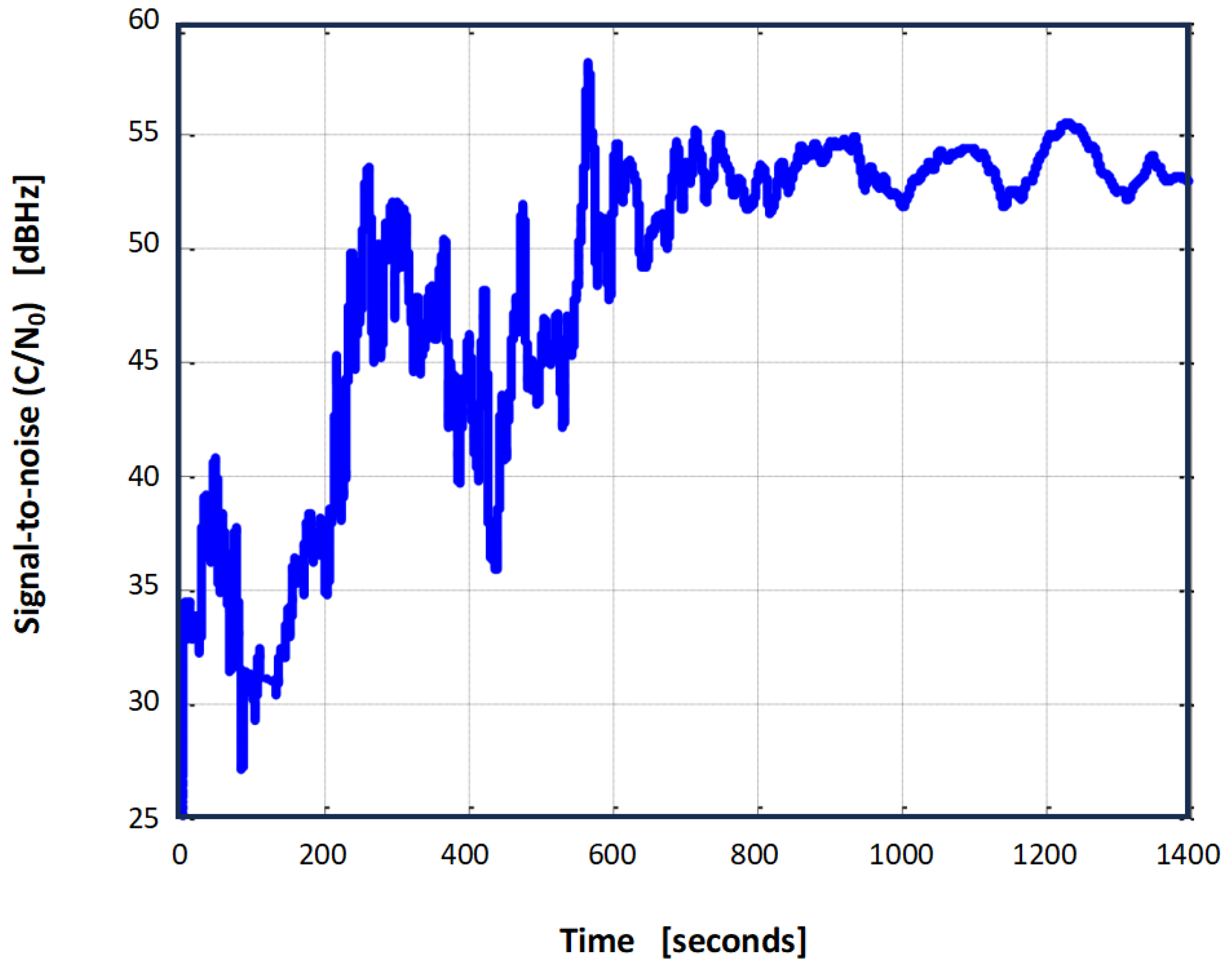
The acquisition of rising occultations is much more demanding than acquiring setting occultations measurements because the autonomous search for the GNSS signal is started before it exists in the receiver. Calculations based on the known GNSS satellite orbits, positions, and the applied Doppler model, leads to sets of code phase delays, which continuously are tested against the measured signal power. The code phase delay with the largest signal energy is then chosen and verified. This tracking strategy has a success rate of 97% once the signal-to-noise power density C/N0 is high enough. Figure 2 shows the measured C/N0 for a rising GNSS satellite. The instrument acquires the signal at 30 dBHz and keeps tracking L1 and L2 phase and code as long as the signal is larger than this value.
The receiver normally tracks the L1 (C/A)-code from below the surface defined by the measured signal-to-noise level and straight-line tangent altitude. This continues until the GNSS satellite disappears from within the opening angle of the receiving antenna. Measurements of the L1/L2 P(Y)-code signals are activated above the atmosphere boundary layer. The receiver tracks in parallel both L1 and L2 phase signals using semi-codeless tracking and L1 signals in open-loop mode. In open loop tracking, the signal is down-converted using a numerically controlled oscillator, which generates a frequency given by the onboard Doppler model. The baseband signal is then sampled at a rate of 1000 Hz.
The characteristics of the reflected signal depend on the scattering properties of the sea surface and the footprint of the reflection zone. The footprint shape and size in turn depend on the signal incidence angle and the relative velocities of the transmitter and the receiver. In our experiments, the receiver was fixed on the mountain, while the transmitter was moving slowly during the grazing angle measurements. Thus, scattering properties of the sea surface in this setup are directly related to the sea surface roughness, which again depends on sea wave characteristics. Due to the geometry, at low elevation grazing angles, the received GPS signals do also contain the incoherent scattering processes taking place in the lower boundary layer and the reflection zone [20]. A longer distance between the receiver and the reflection zone, and a higher altitude of the receiver reduce the effect of incoherent phenomena in the measurements. Additionally, when the receiver is at higher altitudes, the straight-line tangent altitude defining the power spectral information is less influenced by atmospheric turbulence.
The measurement campaign was conducted in the period from 4 October to 13 October 2004. A total of 95 occultations were successfully recorded during the campaign, having almost vertical tracks with respect to the ocean surface. According to a buoy, located southwest of Hawaii (17.14°N; 157.79°W), the mean surface wind speed (averaged over 5 min) varied between 2 m/s and 15 m/s during the period. All meteorological data for the reflection zone used in the paper originate from the US National Weather Service, NOAA.
The GPS receiver was operating in a 1000 Hz sampling mode using the open-loop approach [19,21]. In addition to the direct GPS signal, having the highest power, the calculated sliding power spectra also identified the ocean reflected signal. This occurred from elevation angles (lower than 3 degrees) down to −4 degrees, primarily due to the geometry of the experiment. The reflected signal from each GPS satellite was monitored in a time window of about 20–30 min. During this period, the ocean reflection zone moved horizontally by less than a few hundred meters. For the lower grazing angles and higher wind fields, the reflection zone widened, forming an elliptical shape of the interaction zone. Power spectra of the measured antenna in-phase (I) and quadrature (Q) amplitude components showed this effect as a spectral broadening of the main signal.
3. Determination of Sea Surface Roughness from Measurements
The Rayleigh roughness parameter is widely used to estimate the degree of roughness in ocean remote sensing of electromagnetic wave scattering from rough surfaces. It is a qualitative estimation of the processes in the reflection zone.
The electromagnetic roughness of a surface is directly related to the phase variations of the reflected field caused by surface height variations. Thus, it is the phase variations of the reflected field around its mean value that need be considered.
The electromagnetic scattered wave field Er can be split into the mean <Er> and fluctuating term δEr of the field, where the latter represents the incoherent part of the signal. The total wave field intensity scattered by the surface becomes:
The first term on the right-hand side represents the coherent intensity, corresponding to the reflection from an almost perfectly flat surface. The second term is the incoherent intensity, due to angular spreading and its weak correlation with the incident wave. The coherent term is largest for small surface height variations and the incoherent term vanishes. For larger ocean waves and winds fields, the coherent term is damped, while the incoherent term increases. Thus, for rough ocean surfaces the incoherent term dominates the electromagnetic scattered wave field, and the coherent term can be neglected.
The Rayleigh roughness parameter is related to the coherent scattered intensity (first term on the right-hand side of Equation (1)). It can be shown that the average reflected scattered field intensity |<Er >|2 can be expressed as follows [22]:
The term |E0|2 corresponds to the reflection from a perfectly flat surface, while the second term describes the surface electromagnetic roughness averaged over all surface heights in the reflection zone, equaling the attenuation of the coherent intensity due to the surface roughness.
For a Gaussian density probability distribution of the ocean heights in question, the second right-hand term becomes , with RA is the Rayleigh roughness parameter associated with the reflected wave. Thus, RA can be shown to be equal to:
The Rayleigh roughness parameter, obtained from the root mean square of the phase variations, is a useful and good estimator for assessing the surface roughness of the received electromagnetic signal [22,23,24].
A well-developed sea, forced by a wind speed U, generates a wave spectrum for the air–sea interaction [23,25,26]. A first-order approximation model to the high-wave-number part of the power spectra states that the mean ocean wave-height h is proportional to the square of the wind speed U as given in the Equation (4) [20,23,26,27]. However, short waves are also linked to intermediate and long-scale waves. Thus, a more elaborate spectral model needs to be applied for assessing these processes and the full development of high and low wave numbers of ocean waves. Here, it was omitted in order to simply the retrieval of the ocean sea roughness parameter.
C1 is a constant that, in our calculations, was set to 0.0051 [20]. On the basis of the geometry of the position of the GPS satellite and the GPS receiver, and through the use of Equation (4), it is possible to calculate the rough surface impedance and the rms Rayleigh roughness parameter from the wind speeds. The latter is directly related to the variances in the measured signal power spectra (Equation (3)).
The experimental geometry (Figure 1) limits the number of reflection zones that is visible for the receiver. The GPS receiver (Rx) is fixed on the Hawaiian mountain looking toward south-southwest with the main lobe of the antennas centered on the rim of the horizon. The GPS satellites (Tx) have rising and setting paths on the sky, which for most cases has a sloping angle with respect to the horizon. The time the GPS receiver is able measure GNSS-R signals varies from 20 min to several hours depending on the skewness of the track in the sky [28]. Satellite tracks off from the vertical result in movements of the reflection zone on the ocean. Thus, we selected only GPS satellite tracks that were close to the vertical with respect to the ocean surface. Such situations gave the shortest observation time of ocean reflected signals and made the temporal analysis of the observations more stringent. The data presented in Figure 3 is from such a situation.
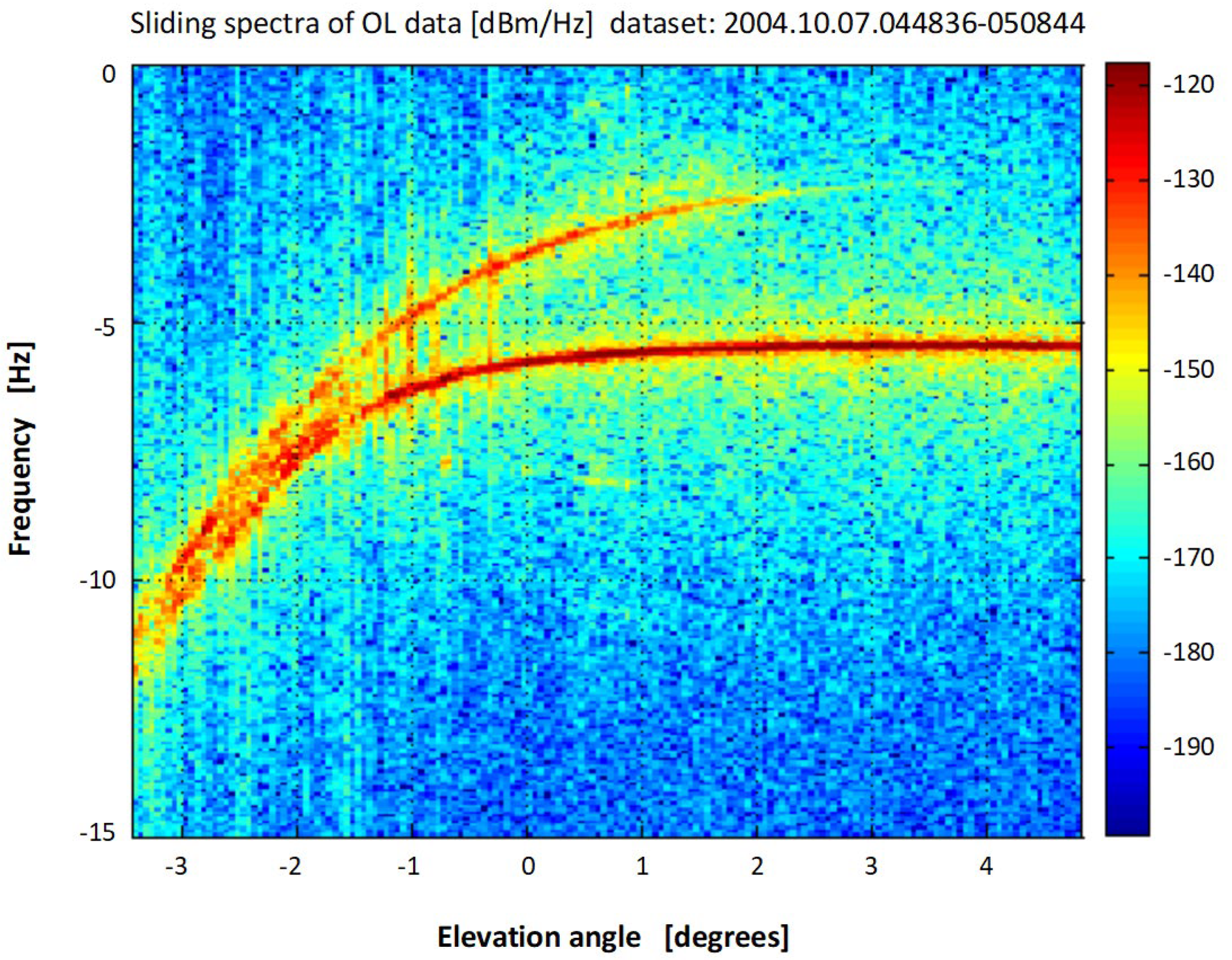
Figure 3 shows the measured signal power spectra as function of time for the direct and the reflected GPS signal. Here, time on the x-axis is transformed into elevation angle. The stack-plot presentation of the spectral content clearly identifies the direct signal for elevation angles spanning from −3.5° to 5.0°. The track of the direct GPS signal (Rx) is horizontal in the plot from 0.0° to 5.0°. The trace above the direct GPS trace is the ocean reflected signal, which shows up as a significant peak in the power spectra. The direct and reflected signals traces are observed for negative frequencies in the power spectra (y-axis of Figure 3). This delay is primarily due to the bending of the GNSS signal in the ionosphere and troposphere compared to the power at the straight-line tangent altitude [17,20]. A negative straight-line tangent altitude refers to the situation when the transmitting GNSS satellite is below the horizon with respect to the receiver. The negative offset in the Doppler model is continuously calculated based on real-time navigation and GNSS ephemerides, and it is included in the retrieval of the amplitude and phase of the sampled signal [17].
The atmospheric conditions in the troposphere during the measurement period in Figure 3 showed slowly varying surface wind fields of 5–10 m/s with high humidity in the boundary layer of the troposphere. Thus, it was a quiet period with constant wave height fields (in a statistical sense).
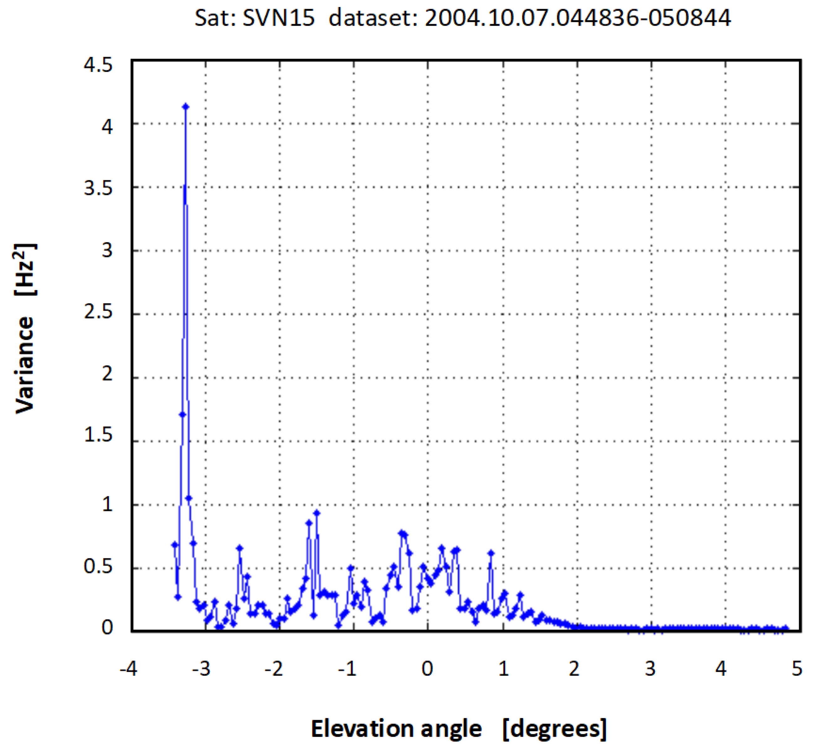
Figure 4 presents the associated variances, centered on the maximum mean power of the ocean reflected trace given in Figure 3. For all elevation angles the variances are below 1 Hz2 and no changes are observed due to the less than half a kilometer movement of the reflection zone during the observations. The power spectra show a distinct peak centered on the reflected signal trace following a Gaussian distribution function. This is the case for all elevations angles given in Figure 4.
The spike in the figure for elevation angles less than −3.1 degrees occurs when the peak of the reflected trace descends into or arises from the noise floor. The variances becomes large due to this effect independent of the frequency range. The power in the reflected signal is here low and of the order of the noise level.
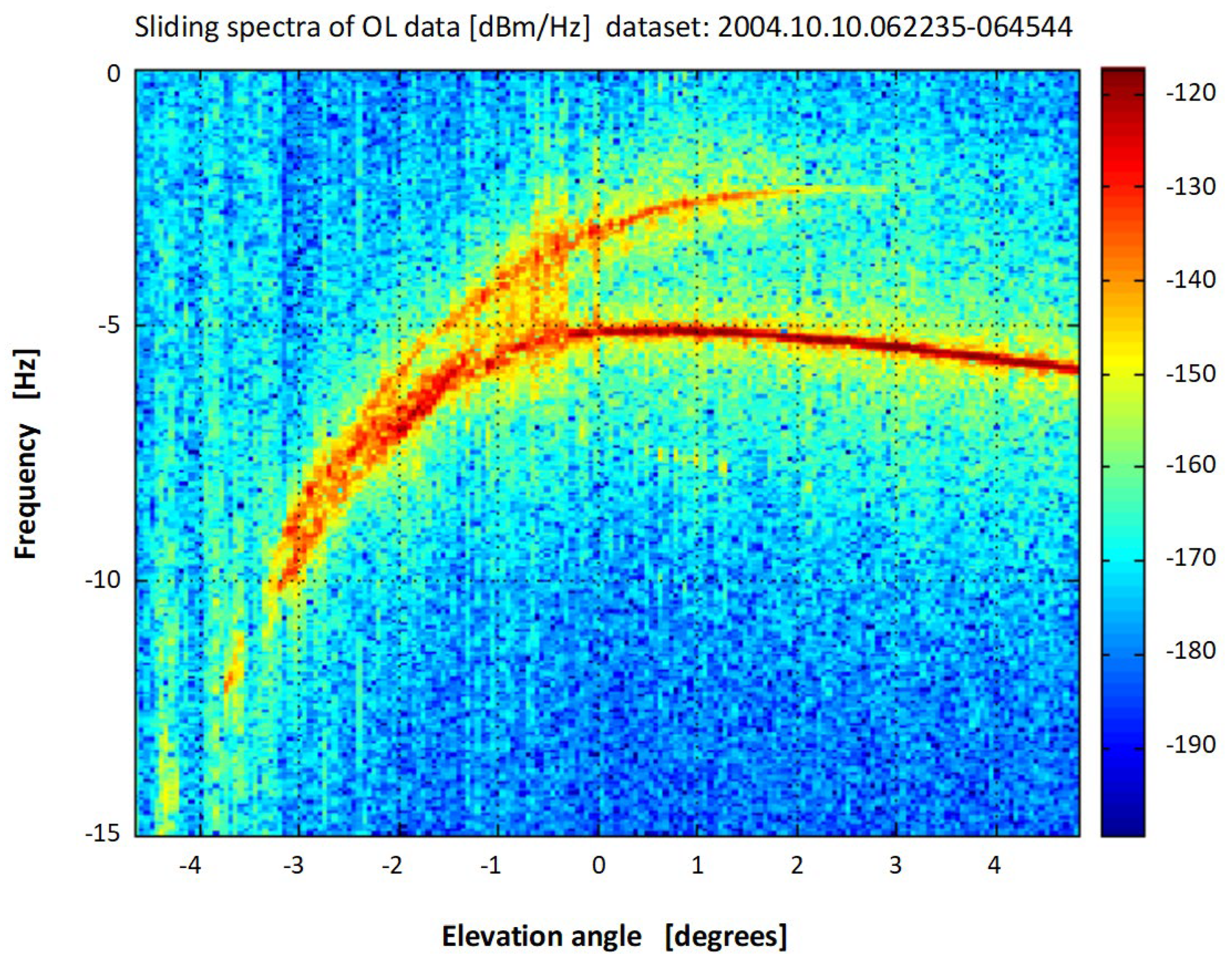
Figure 5 shows such conditions, where the reflected signal is submerged into the broad-band noise of the power spectra. This occurs for elevations from −3.2 degrees to −4.6 degrees. In this period the variance gave values from 7 Hz2 and up to 20 Hz2.
The obtained variances applied in all data retrievals have a temporal resolution of 0.1 Hz. Shorter sampling intervals for acquiring the variances have been tested too. Applying 1, 10, and 50 Hz sampling intervals for calculating the variances gave higher variance values mainly due the wide-band noise in the observations. Thus, a 0.1 Hz sampling rate were chosen to minimize this effect. For all the applied sampling intervals the envelope of the variances had the same fixed form and was only shifted by a constant value. Thus, the variance as function of the sampling interval gave only a constant increase independent of the elevation angle and the sea state.
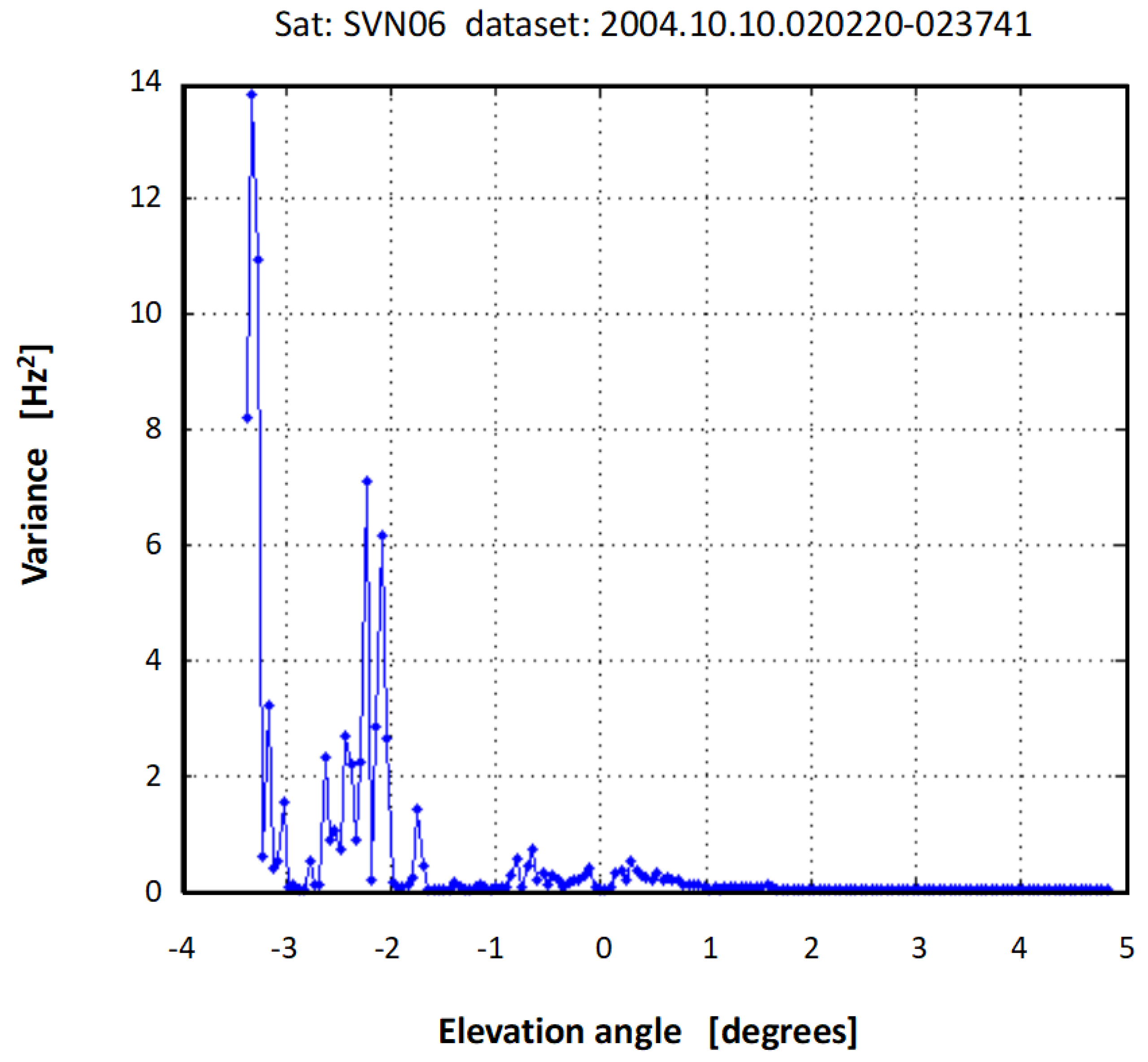
For higher ocean surface winds (larger above 10 m/s) the variances became significantly larger. Figure 6 shows the variances for conditions when the mean wind field ranges from 10 m/s to above 15 m/s. The large peak for elevation angles below −3.1 degrees are also here due to the fact that the maximum power of the reflected trace is of the order of the noise power in the measurements.
All datasets showing higher mean winds reveal also larger variations in the variances. For example, the variances in Figure 6 change from less than 1 Hz2 to 7 Hz2 during a five-minute period for elevation angles going from −1.5 degrees to −3.0 degrees. Here, this may be due to directional changes in the horizontal wind vectors. The meteorological observations and data from a nearby buoy partly support this explanation. But other phenomena need to be considered for understanding the full picture of these variations. Among them are, atmosphere turbulence in the lower boundary layer of the troposphere, ocean evaporation processes, and vertical components of the troposphere wind fields.
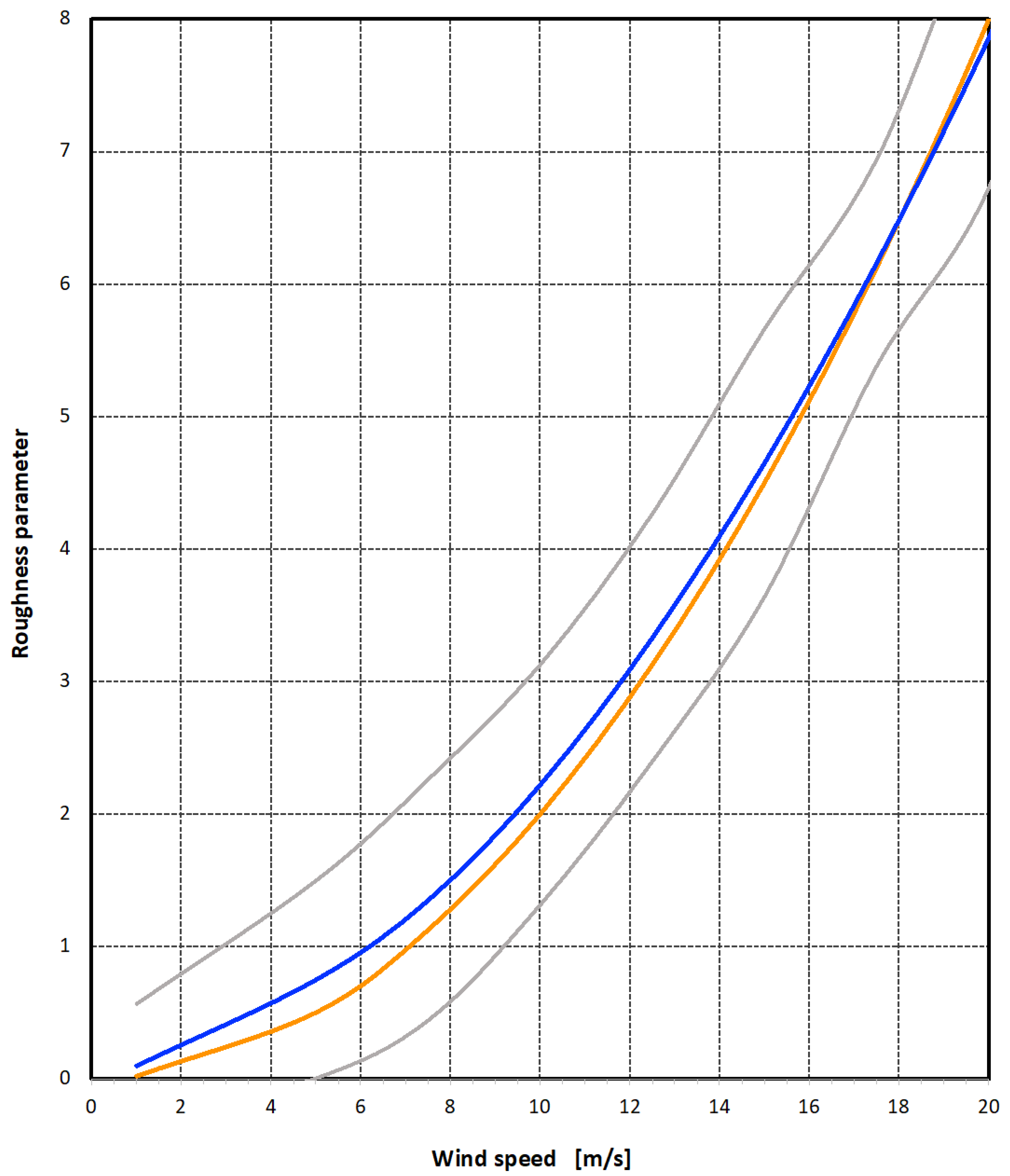
In the next step, we retrieved the roughness parameter from the mean variance ratio between the reflected and direct signals evaluated for elevation angles in the range from −3.0° to +2.0°. Figure 7 shows the derived rms Rayleigh roughness parameters as a function of wind speed based on all the GNSS-R measurements. The obtained curves are piecewise cubic polynomial fits to the calculated roughness parameter as a function of the atmospheric surface wind data from the meteorological forecast model. The measurements cover the observational period in October 2004.
The blue graph in Figure 7 represents the mean estimates of all variances from all observations used in the study, while the gray curves represent the envelopes of all variance retrievals. Next to the blue curve is the orange curve, which is the simple model stating that the roughness parameter is proportional to the square of the wind speed [20]. Both the latter graph (orange) and the derived graph for the rms roughness parameter (blue) show a similar shape for the surface wind speed and the ocean roughness.
Note that the agreement between the blue and the orange curve is well within the uncertainty margins indicated by the gray curves. However, for wind speeds up to 15 m/s, the simple relation seems to underestimate the Rayleigh roughness parameter (RA) compared to the observations presented here by the polynomial fit function (blue curve). This can be explained by the fact that RA is linked to the coherent part of the electromagnetic reflected signal, as described above. For the high-wind domain, the incoherent part of the signal is the dominant cause of GPS waves reflected from the ocean surface [22,24].
4. Scatterometry Simulations of Ocean Reflected GPS Signals, Sea Surface Roughness, and Wave Heights
The wave propagation is performed using a solution to the parabolic equation approximation to the electromagnetic wave equation [14,16,25,29,30]. The parabolic equation in the simulator is solved using the split-step sine transformation, where the Earth’s surface is modeled using an impedance model [20,27,30,31]. This impedance concept gives an accurate lower boundary condition in the determination of the electromagnetic field. The ocean waves are characterized by a semi-isotropic Phillips spectrum [23,26]. In the simulator, this field is represented as the amplitude and the phase of the waves as a function of time, corresponding to the in-phase I and the quadrature Q components [20,32].
The multiphase screen wave propagation uses a detailed refractivity model for the neutral atmosphere, the boundary layer, and the ionosphere. The ionosphere is modeled by the NeQuick model [33]. These models make it possible to simulate multipath phenomena in the neutral atmosphere and scintillations in the ionosphere.
The mixed Fourier transformation and the impedance for rough surfaces (ocean waves) are used to describe the interacting between the electromagnetic wave and the ocean [16]. Equation (5) relates the rough surface impedance δ to the smooth surface impedance δ0 [20].
Values of the smooth surface impedance can be found in the literature for different radio wave frequencies and polarizations [34]. θ in Equation (5) is the angle between the wave vector and ground, known as the grazing angle. The symbol for the roughness reduction factor is ρ. The roughness reduction factor can be expressed as a function of the Rayleigh roughness parameter using the following equation:
where I0 is the modified Bessel function of the first kind of order 0, while the Rayleigh roughness parameter γ is given by the following expression:
where k is the wave number of the electromagnetic wave, while h is the root-mean-square (rms) height of the ocean waves. It is possible to relate the rms of the ocean wave-heights to the wind speed. A detailed analysis of this can be found in [34].
The electromagnetic field at the antenna of the GPS receiver is composed of both a direct wave from the GPS satellite and an ocean reflected wave. The simulations in this study were performed using the L5 GPS signal, having a frequency of 1176.45 MHz. The output from the wave propagator constitutes the amplitudes and phases of the received GPS signal as function of time.
The observations presented in the previous section used the L1 and the L2 GPS signals for the data retrievals (L1: 1575.42 MHz; L2: 1227.60 MHz). Earlier studies have shown no significant changes when using L5 rather than L1 or L2 in the simulations for the estimated ocean wave heights and surface roughness.
Short-time Fourier transforms (spectrograms) were applied to the simulated I and Q signals using the meteorological conditions in the 95 cases [24,25,32,35]. The total field decrease as expected for an increasing elevation angle and the boundaries of the reflected field become relatively sharp [24,34,35,36]. It is also seen, for given spectral values, that the corresponding frequency increases as a function of wind speed and ocean wave-height [24,25,32].
The spectrograms reveal signs of both the reflected and the direct wave, due to a small difference in the frequencies of the direct and reflected waves, as also shown for the observations in Figure 3.
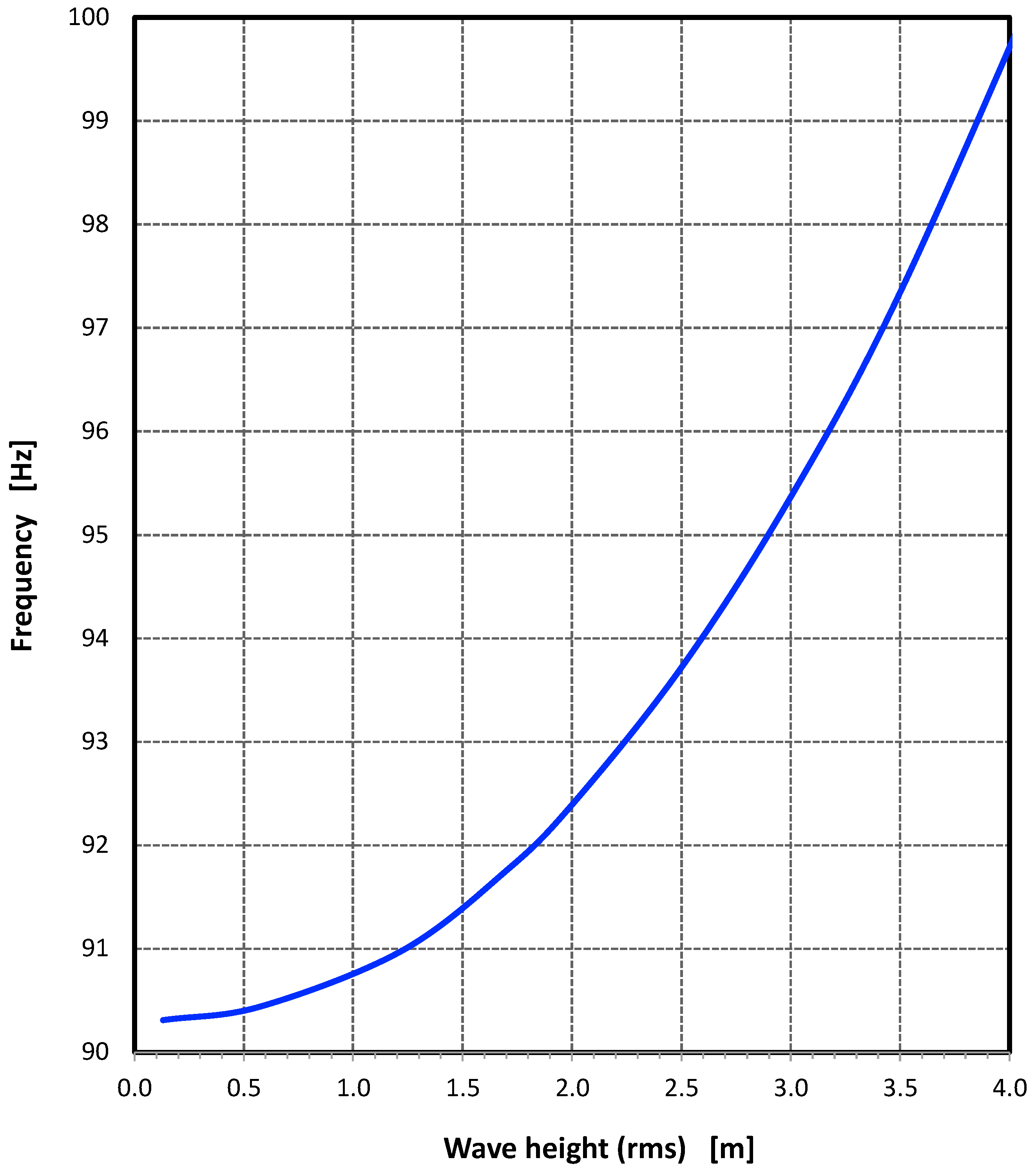
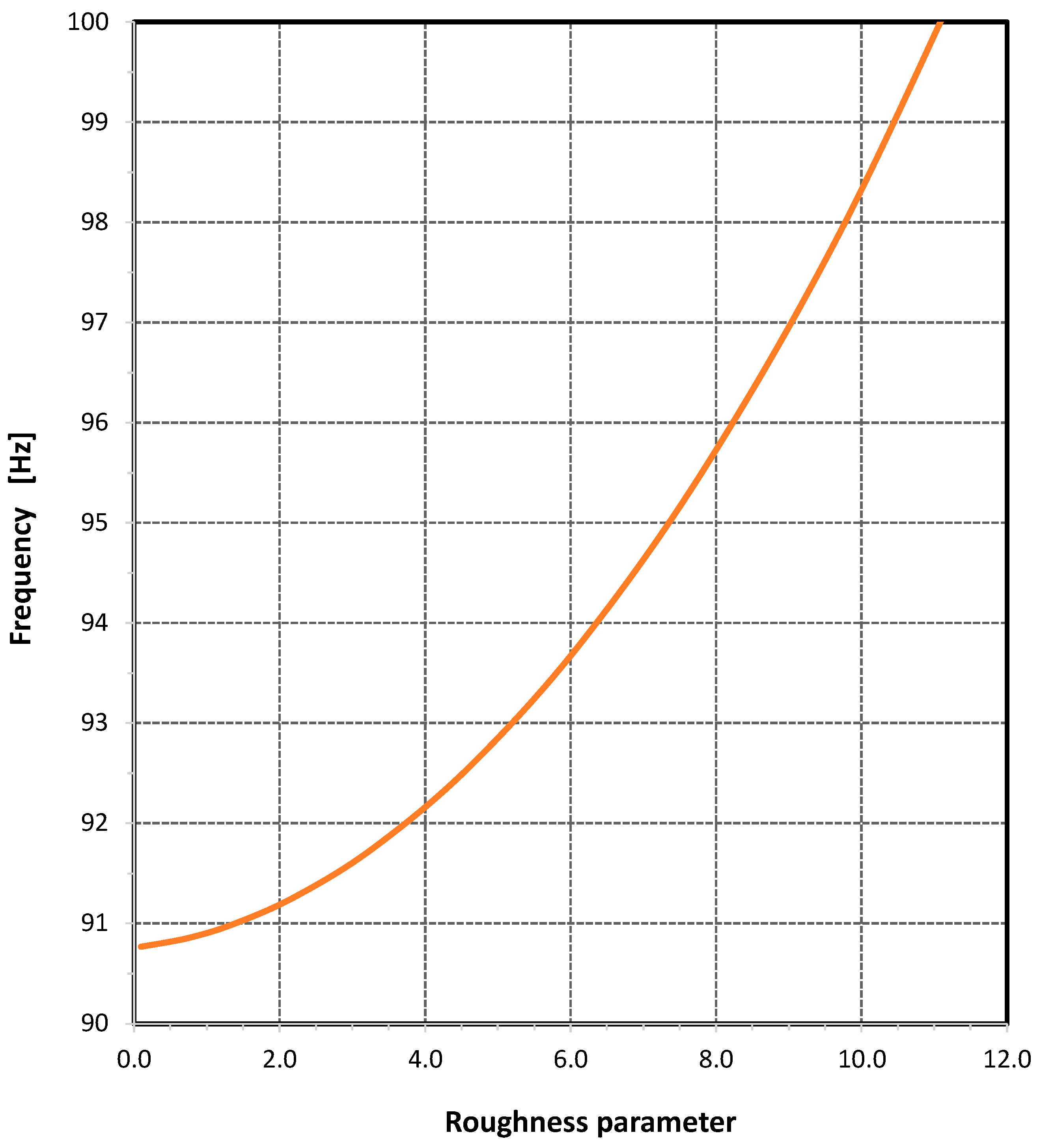
The power spectra in a semi-logarithmic presentation are very close to a straight line with decreasing power for increasing frequency. However, the ocean rms wave-height, as a function of the spectral frequency in a given spectral domain, shows increasing Rayleigh roughness as a function of frequency. Here the Rayleigh roughness parameters are calculated from the rms wave-heights [20,27,29]. Figure 8 and Figure 9 show how wave-heights and ocean roughness relate to the spectral frequency in the chosen frequency band.
The retrieval method builds on the knowledge that the power spectrum has an almost linear slope for the chosen frequency range [20]. The frequency f0 (in Equations (8) and (9)) becomes a constant (determined by the chosen frequency range in the power spectrum) and changes with respect to the used wave heights and surface winds (sea states). Thus, the simulated spectra can be fitted by the function W:
where f represents a frequency in the frequency band in question, and f0 is a constant frequency related to the parameters used in the simulations. The function W is similar to the spectrum model applied in the paper [29].
It should be noted that, when the spectrum model above is used to fit the simulated spectra, an extra constant value has to be added to the model. In our simulations, a spectral value of 33 dB was used for producing the results shown in Figure 8 and Figure 9. The outcome shows clearly that the power spectral values increase as function of wind speed and ocean wave-height.
A typical statistical value of R2 for the applied retrieval process was 0.988, meaning that approximately 98% of the variations can be explained by the spectrum model.
For most frequency bands (from 0.1 to 500 Hz), the relation of the rms wave-height, roughness, and the spectral frequency follows a hyperbolic relation of the following form:
where f and f0 are spectral frequencies in the frequency band as explained above, and C0 is a constant. The eccentricity, ε, of the hyperbola is given by the major axis, a, and the minor axis, b, of the hyperbolic function.
In the simulations, ε varies for increasing spectral frequency, and it is also a function of the distance between the phase screens. Thus, for the higher spectral frequencies, ε may be linked to the turbulence cascading process between the longer- and shorter-wavelength waves.
5. Discussion
The combination of GNSS-R data retrievals and computer simulations of ocean wave height and sea surface roughness supported our knowledge of the significance in identifying the characteristics of sea states by measuring GNSS reflected signals. For surface winds up to 20 m/s, the trace followed a close-to-Gaussian power density distribution. The associated variances based on the running mean value of the trace lead to the retrieval of ocean wave heights and surface roughness that are close to the theoretical values calculated from the equations and simulations. The changes in the variances of the reflected trace for higher wind fields seems to be driven by horizontal wind directional changes. This effect was partly supported by wind field data from an NWP model. But other phenomena as troposphere turbulence may also be a candidate for the changes, which occurs within minutes.
One of the advantages of the measurement setup is that the ocean reflection zone is observed for periods of up to 30 min, primarily due to the geometry of the experiment for each GNSS satellite in view of the antenna. Having more antennas, looking in different directions, and receiving signals from several global satellite systems would increase the knowledge of winds, ocean wave height spectra, surface heights (altimetry), and sea surface roughness over a larger area of the ocean. The GNSS-R observations could further be an important contribution to long-term variations of the ocean mean height, as well as the monitoring of ocean mesoscale eddies (with spatial features of 100 km and temporal variability of the order of several days), which result in sea height changes much larger than the accuracy of the GNSS-R technique.
The number of measurements in each wind speed bin is not equal. Most of the measurements lie in the wind velocity bins from 2 m/s to 10 m/s. Thus, the goodness of fit of the spectral information content results in skewed errors for the higher wind fields.
The paper also presented the theory and models needed to describe the interaction between the electromagnetic field emitted from a GNSS satellite and ocean waves. The interaction was modeled through a mixed Fourier transform and an Earth impedance concept [27]. Models of both the neutral atmosphere and the dispersive ionosphere were also included to further improve the simulations. These models play an important part in the simulations [20,27]. Especially the bending and the spectral broadening of the GNSS signal for grazing angle measurements impact the received signal at the receiver.
Simulations and GNSS-R measurements of the bistatic system (consisting of the transmitting GPS satellite, reflections from the ocean, and the GPS receiver) were performed for a total of 95 datasets. The slopes of the obtained power spectra were directly related to the sea states and, hence, the ocean wave-heights [27]. The simulations also pointed to the fact that the estimates of wave heights and roughness parameters are a function of the spectral domain used for the retrievals. Here, the calculations were done for the frequency range from 90 Hz to 100 Hz, which require an instrument capable of high sampling rates. The instrument in the experiments used an open-loop technique with a sampling rate of 1000 Hz. The advantage of this approach is very detailed I and Q measurements that is not hampered by internal instrumental clock errors or the chosen phase-locked loop approach in the receiver. At the same it is possible to analyze atmospheric modulation and GNSS co-channel interference from other GNSS satellites. The Doppler model guiding the open-loop measurements proved to be accurate enough for obtaining the needed spectral resolution that can distinguish the direct and the ocean reflected GNSS signals. To minimize clock errors in the instrument an atomic clock was applied to steer the oscillators of the receiver. Thus, ocean surface measurements can be dependent on the type and the quality of the applied GNSS-R receiver.
6. Conclusions
The GNSS-R ocean surface measurements were shown to be a good estimator of sea surface roughness and wave heights in the reflection zone. The grazing angle measurements additionally have the potential of delivering climate change input by monitoring the following ocean phenomena when including signal reception from more GNSS frequency bands from several global navigations systems (GPS, GALILEO, BEIDOU, and GLONASS) [7]:
- Ocean mesoscale eddies and fronts (with horizontal spatial scales of 5–1000 km and temporal scales of 1 day–1 year),
- Mean ocean height variations (horizontal scales of 10–1000 m and temporal scales of 1 h–1 week),
- Ocean surface mean-square slopes/tilts (horizontal scales of 1–100 km and temporal scales of 5–50 h),
- Directional changes in the wind field patterns (horizontal scales of 10 m–100 km and temporal scales of 1 min–10 h).
Combining all these measurements in the field of view of the receiving antennas leads to a range of reflection zones in the vicinity of the reflection zones from the GPS signals, which will have enough resolution to identify the abovementioned parameters and sea conditions.
It was also shown that the signal spectra can be approximated by a relatively simple model, where the model constant is a function of the sea state. The retrieved mean wave-heights are almost proportional to the square of the wind speed, and the spectral variances from the measurements of setting and rising GNSS satellites link directly to the ocean surface roughness. Similar results were obtained in the performed multiphase screen wave propagation simulations. The relationships presented here can be used in practice to estimate sea states and wave-heights.
The field of reflectometry is a relatively new research area with great potential for the retrieval of new and more precise geophysical parameters such as sea surface roughness, wave height, horizontal and vertical wind patterns, ocean tilt, ocean water salinity, ocean heat dissipation and evaporation transport, boundary layer humidity, and lower-troposphere turbulence. This great potential can also be seen from the relatively large number of satellite missions emerging in the near future. Thus, it is important to have the necessary tools to perform appropriate simulations and algorithms for assessing the actual performance of the technique, deriving the mentioned geophysical parameters.
The spectral surface model, used here to represent the air–sea interaction, is a relatively simple model. More accurate models should be developed as in [23], making the relationship between wind speed and ocean wave-heights more accurate for both high and low wave numbers. It should also be mentioned that the relations for the smooth and rough impedances given in the paper are approximations to more general expressions. Further measurement campaigns under different geophysical conditions and locations than presented here would strengthen the validating and performance of the presented models and simulation tools.
Author Contributions
Both authors contributed to the preparation of the article. Conceptualization, P.H. and A.C.; methodology, P.H. and A.C.; software, P.H. and A.C.; validation, P.H.; formal analysis, P.H.; investigation, P.H.; resources, P.H. and A.C.; data curation, P.H. and A.C.; writing—original draft preparation, P.H. and A.C.; writing—review and editing, P.H. and A.C.; visualization, P.H.; supervision, P.H.; project administration, P.H.; funding acquisition, P.H. and A.C. All authors have read and agreed to the published version of the manuscript.
Funding
The research was made available by internal grants at University of Oslo, Norway, and the company Beyond Gravity, Sweden.
Data Availability Statement
Measurements from the five datasets are available upon request to the authors.
Acknowledgments
The authors want to acknowledge Wojciech Miloch, University of Oslo, Department of Physics, in Norway for his support to the research necessary for obtaining the results in the article. The assistance of the University of Hawaii in realizing the observations is very much appreciated. This work was supported by the Swedish National Space Board and the Danish Technical Research Council. The authors also acknowledge the Swedish National Testing and Research Institute for providing the rubidium atomic clock.
Conflicts of Interest
The authors declare no conflict of interest.
References
- Cardellach, E.; Fabra, F.; Noguès-Correig, O.; Oliveras, S.; Ribò, S.; Rius, A. GNSS-R ground based and airborne campaigns for ocean, land, ice, and snow techniques: Application to the GOLD-RTR data sets. Radio Sci. 2011, 46, RS0C04. [Google Scholar] [CrossRef] [Green Version]
- Cardellach, E.; Ao, C.O.; de la Torre Juàrez, M.; Hajj, G.A. Carrier phase delay altimetry with GPS-reflection/occultation interferometry from low Earth orbiters. Geophys. Res. Lett. 2004, 31, L10402. [Google Scholar] [CrossRef]
- Rius, A.; Aparicio, J.M.; Cardellach, E.; Martin-Neira, M.; Chapron, B. Sea surface state measured using GPS reflected signals. Geophys. Res. Lett. 2002, 29, 2122. [Google Scholar] [CrossRef] [Green Version]
- Rodriguez-Alvarez, N.; Munoz-Martin, J.F.; Morris, M. Latest Advances in the Global Navigation Satellite System-Reflectometry (GNSS-R) Field. Remote Sens. 2023, 8, 2157. [Google Scholar] [CrossRef]
- Unwin, M.J.; Pierdicca, N.; Cardellach, E.; Rautiainen, K.; Foti, G.; Blunt, P.; Guerriero, L.; Santi, E.; Tossaint, M. An Introduction to the HydroGNSS GNSS Reflectometry Remote Sensing Mission. IEEE J. Sel. Top. Appl. Earth Obs. Remote Sens. 2021, 14, 6987–6999. [Google Scholar] [CrossRef]
- Unwin, M.; Jales, P.; Tye, J.; Gommenginger, C.; Foti, G.; Rosello, J. Spaceborne GNSS-Reflectometry on TechDemoSat-1: Early Mission Operations and Exploitation. IEEE J. Sel. Top. Appl. Earth Obs. Remote Sens. 2016, 9, 4525–4539. [Google Scholar] [CrossRef]
- Wickert, J.; Cardellach, E.; Martin-Neira, M.; Bandeiras, J.; Bertino, L.; Andersen, O.B.; Camps, A.; Catarino, N.; Chapron, B.; Fabra, F.; et al. GEROS-ISS: GNSS Reflectometry, Radio Occultation and Scatterometry onboard the International Space Station. IEEE J. Sel. Top. Appl. Earth Obs. Remote Sens. 2016, 9, 4552–4581. [Google Scholar] [CrossRef] [Green Version]
- Foti, G.; Gommenginger, C.; Jales, P.; Unwin, M.; Shaw, A.; Robertson, C.; Rosello, J. Spaceborne GNSS reflectometry for ocean winds: First results from the UK TechDemoSat-1 mission. Geophys. Res. Lett. 2015, 42, 5435–5441. [Google Scholar] [CrossRef] [Green Version]
- Ruf, C.; Lyons, A.; Unwin, M.; Dickinson, J.; Rose, R.; Rose, D.; Vincent, M. CYGNSS: Enabling the Future of Hurricane Prediction. IEEE Geosci. Remote Sens. Mag. 2013, 1, 52–67. [Google Scholar] [CrossRef]
- Fong, C.-J.; Yen, N.L.; Chang, G.-S.; Cook, K.; Wilczynski, P. Future Low Earth Observation Radio Occultation Mission: From Research to Operations. In Proceedings of the 2012 IEEE Aerospace Conference, Big Sky, MT, USA, 3–10 March 2012. [Google Scholar]
- Wickert, J.; Beyerle, G.; Cardellach, E.; Förste, C.; Gruber, T.; Helm, A.; Hess, M.P.; Høeg, P.; Jakowski, N.; Montenbruck, O.; et al. GNSS Reflectometry, Radio Occultation and Scatterometry onboard ISS for long-term monitoring of climate observations using innovative space geodetic techniques on-board the International Space Station. In Proposal in Response to Call: ESA Research Announcement for ISS Experiments Relevant to Study of Global Climate Change; European Space Agency (ESA): Noordwijk, The Netherlands, 2011. [Google Scholar]
- Beyerle, G.; Hocke, K. Observation and simulation of direct and reflected GPS signals in radio occultation experiments. Geophys. Res. Lett. 2001, 28, 1895–1898. [Google Scholar] [CrossRef]
- Wait, J.R. Review of mode theory of radio propagation in terrestrial waveguides. Rev. Geophys. 1963, 1, 481–505. [Google Scholar] [CrossRef]
- Kerr, D.E. Propagation of Short Radio Waves; Dover Publications: New York, NY, USA, 1951. [Google Scholar]
- Tatarskii, V.I. Wave Propagation in a Turbulent Medium; MacGraw-Hill: New York, NY, USA, 1961. [Google Scholar]
- Kuttler, J.R.; Dockery, G.D. Theoretical description of the parabolic approximation/Fourier split-step method of representing electromagnetic propagation in the troposphere. Radio Sci. 1991, 26, 381–393. [Google Scholar] [CrossRef]
- Bonnedal, M.; Christensen, J.; Carlström, A.; Berg, A. METOP-GRAS in-orbit instrument performance. GPS Solut. 2009, 14, 109–120. [Google Scholar] [CrossRef]
- Olsen, L.; Carlström, A.; Høeg, P. Ground Based Radio Occultation Measurements Using the GRAS Receiver. In Proceedings of the Proceedings of the 17th International Technical Meeting of the Satellite Division of The Institute of Navigation (ION GNSS 2004), Long Beach, CA, USA, 21–24 September 2004; pp. 2370–2377. [Google Scholar]
- Carlstrom, A.; Emardson, R.; Christensen, J.; Sinander, P.; Zangerl, F.; Larsen, G.B.; Hoeg, P. The GPS Occultation Sensor for NPOESS. In Proceedings of the IEEE International Geoscience and Remote Sensing Symposium, Toronto, ON, Canada, 24–28 June 2002; Volume 1, pp. 553–555. [Google Scholar]
- Benzon, H.-H.; Høeg, P.; Durgonics, T. Analysis of satellite-based navigation signal reflectometry: Simulations and observations. IEEE J. Sel. Top. Appl. Earth Obs. Remote Sens. 2015, 9, 4879–4883. [Google Scholar] [CrossRef]
- Høeg, P.; Prasad, R.; Borre, K. Impact of atmosphere turbulence on satellite navigation signals. In Satellite Communications and Navigation Systems; Del Re, E., Ruggieri, M., Eds.; Springer: Berlin/Heidelberg, Germany, 2008; pp. 231–239. [Google Scholar] [CrossRef]
- Pinel, N.; Bourlier, C.; Saillard, J. Degree of roughness of rough layers: Extensions of the Rayleigh roughness criterion and some applications. Prog. Electromagn. Res. B 2010, 19, 41–63. [Google Scholar] [CrossRef] [Green Version]
- Elfouhaily, T.; Chapron, B.; Katsaros, K. A unified directional spectrum for long and short wind-driven waves. J. Geophys. Res. 1997, 102, 15781–15796. [Google Scholar] [CrossRef] [Green Version]
- Beckmann, P.; Spizzchino, A. The Scattering of Electromagnetic Waves from Rough Surfaces; Artech House: London, UK, 1987. [Google Scholar]
- Zavorotny, V.U.; Voronovich, A.G. Scattering of GPS Signals from the Ocean with Wind Remote Sensing Application. IEEE Trans. Geosci. Remote Sens. 2000, 38, 2. [Google Scholar] [CrossRef] [Green Version]
- Phillips, O.M. On the generation of waves by turbulent wind. J. Fluid Mech. 1957, 2, 417–445. [Google Scholar] [CrossRef]
- Benzon, H.-H.; Høeg, P. Wave propagation simulation of radio occultations based on ECMWF refractivity profiles. Radio Sci. 2015, 50, 778–788. [Google Scholar] [CrossRef]
- Høeg, P.; Carlström, A. Information content in reflected global navigation satellite system signals. In Proceedings of the 2011 2nd International Conference on Wireless Communication, Vehicular Technology, Information Theory and Aerospace & Electronic Systems Technology (Wireless VITAE), Chennai, India, 28 February–3 March 2011; IEEE: New York City, NY, USA, 2011; Volume 1. Available online: https://0-ieeexplore-ieee-org.brum.beds.ac.uk/abstract/document/5940894 (accessed on 19 July 2023).
- Ungan, B.U.; Johnson, J.T. Time Statistics of Propagation over the Ocean Surface: A Numerical Study. IEEE Trans Geosci. Remote Sens. 2000, 38, 4. [Google Scholar] [CrossRef]
- Collins, M.D. A two-way parabolic equation for acoustic backscattering in the ocean. J. Acoust. Soc. Am. 1992, 91, 1357–1358. [Google Scholar] [CrossRef]
- Barclay, L. Propagation of Radiowaves; The Institution of Engineering and Technology: London, UK, 2003. [Google Scholar]
- Pavelyev, A.G.; Zhang, K.; Matyugov, S.S.; Liou, Y.A.; Wang, C.S.; Yakovlev, O.I.; Kucherjavenkou, I.A.; Kuleshov, Y. Analytical model of bi-static reflections and radio occultation signals. Radio Sci. 2011, 46, RS1009. [Google Scholar] [CrossRef]
- Nava, B.; Coisson, P.; Radicella, S.M. A new version of the NeQuick ionosphere electron density model. J. Atmos. Sol.-Terr. Phys. 2008, 83, 47–53. [Google Scholar] [CrossRef]
- Haynes, W.M. CRC Handbook of Chemistry and Physics, 93rd ed.; CRC Press: Boca Raton, FL, USA, 2012; ISBN 9781439880494. [Google Scholar]
- Beyerle, G.; Hocke, K.; Wickert, J.; Schmidt, T.; Marquardt, C.; Reigber, C. GPS radio occultations with CHAMP: A radio holographic analysis of GPS signal propagation in the troposphere and surface reflections. J. Geophys. Res. 2002, 107, 4802. [Google Scholar] [CrossRef] [Green Version]
- Boashash, B. Time Frequency Signal Analysis and Processing: A Comprehensive Reference; Elsevier: Oxford, UK, 2003. [Google Scholar]
Figure 1.
The transmitted wave from the GNSS satellite (Tx) in blue is reflected at the ocean surface and received by the GNSS receiver (Rx). The red line represents the direct GNSS signal path.
Figure 1.
The transmitted wave from the GNSS satellite (Tx) in blue is reflected at the ocean surface and received by the GNSS receiver (Rx). The red line represents the direct GNSS signal path.

Figure 2.
Signal-to-noise ratio (C/N0) as function of time for a rising GPS satellite. The measurements originate from 4 October 2004 (6:56–7:21 UTC).
Figure 2.
Signal-to-noise ratio (C/N0) as function of time for a rising GPS satellite. The measurements originate from 4 October 2004 (6:56–7:21 UTC).

Figure 3.
Stacked power spectra as function of the elevation (GPS SVN15). The spectra reveal the direct GPS signal and the ocean reflected backscattered GPS signal. The latter is here observed for elevations angles from −3.5° to 3.0°. Observations originate from 7 October 2004 (4:48–5:09 UTC).
Figure 3.
Stacked power spectra as function of the elevation (GPS SVN15). The spectra reveal the direct GPS signal and the ocean reflected backscattered GPS signal. The latter is here observed for elevations angles from −3.5° to 3.0°. Observations originate from 7 October 2004 (4:48–5:09 UTC).

Figure 4.
Retrieved averaged variances (0.1 Hz) for the measurements shown in Figure 3 as a function of the elevation angle.
Figure 4.
Retrieved averaged variances (0.1 Hz) for the measurements shown in Figure 3 as a function of the elevation angle.

Figure 5.
Sliding power spectra as function of the elevation (GPS SVN15). The observations originate from October 10, 2004 (6:22–6:46 a.m. UTC).
Figure 5.
Sliding power spectra as function of the elevation (GPS SVN15). The observations originate from October 10, 2004 (6:22–6:46 a.m. UTC).

Figure 6.
Variances for sea surface states with higher wind fields ranging from 10 m/s to 15 m/s.

Figure 7.
Calculated surface roughness parameters as a function of the observed wind fields for all datasets. The blue curve is the mean estimate of the relation, based on all the observed GPS surface reflection signals and meteorological wind fields in the reflection zone. The gray curves represent the envelopes of all retrieved roughness parameters for all datasets. The orange curve is the relation derived from the above equations.

Figure 8.
Ocean rms wave-height as a function of the spectral frequency in the frequency domain from 90 to 100 Hz.
Figure 8.
Ocean rms wave-height as a function of the spectral frequency in the frequency domain from 90 to 100 Hz.

Figure 9.
The relation between the Rayleigh roughness parameter and the spectral frequency for the same frequency range as in Figure 8. The Rayleigh roughness parameters were calculated for a grazing angle of −1.5°.
Figure 9.
The relation between the Rayleigh roughness parameter and the spectral frequency for the same frequency range as in Figure 8. The Rayleigh roughness parameters were calculated for a grazing angle of −1.5°.

Disclaimer/Publisher’s Note: The statements, opinions and data contained in all publications are solely those of the individual author(s) and contributor(s) and not of MDPI and/or the editor(s). MDPI and/or the editor(s) disclaim responsibility for any injury to people or property resulting from any ideas, methods, instructions or products referred to in the content. |
© 2023 by the authors. Licensee MDPI, Basel, Switzerland. This article is an open access article distributed under the terms and conditions of the Creative Commons Attribution (CC BY) license (https://creativecommons.org/licenses/by/4.0/).
Share and Cite
MDPI and ACS Style
Høeg, P.; Carlström, A. Sea Surface Roughness Determination from Grazing Angle GPS Ocean Observations and Scatterometry Simulations. Remote Sens. 2023, 15, 3794. https://0-doi-org.brum.beds.ac.uk/10.3390/rs15153794
AMA Style
Høeg P, Carlström A. Sea Surface Roughness Determination from Grazing Angle GPS Ocean Observations and Scatterometry Simulations. Remote Sensing. 2023; 15(15):3794. https://0-doi-org.brum.beds.ac.uk/10.3390/rs15153794
Chicago/Turabian StyleHøeg, Per, and Anders Carlström. 2023. "Sea Surface Roughness Determination from Grazing Angle GPS Ocean Observations and Scatterometry Simulations" Remote Sensing 15, no. 15: 3794. https://0-doi-org.brum.beds.ac.uk/10.3390/rs15153794
Note that from the first issue of 2016, this journal uses article numbers instead of page numbers. See further details here.