
Real-Time Terrain Correction of Satellite Imagery-Based Solar Irradiance Maps Using Precomputed Data and Memory Optimization

Abstract
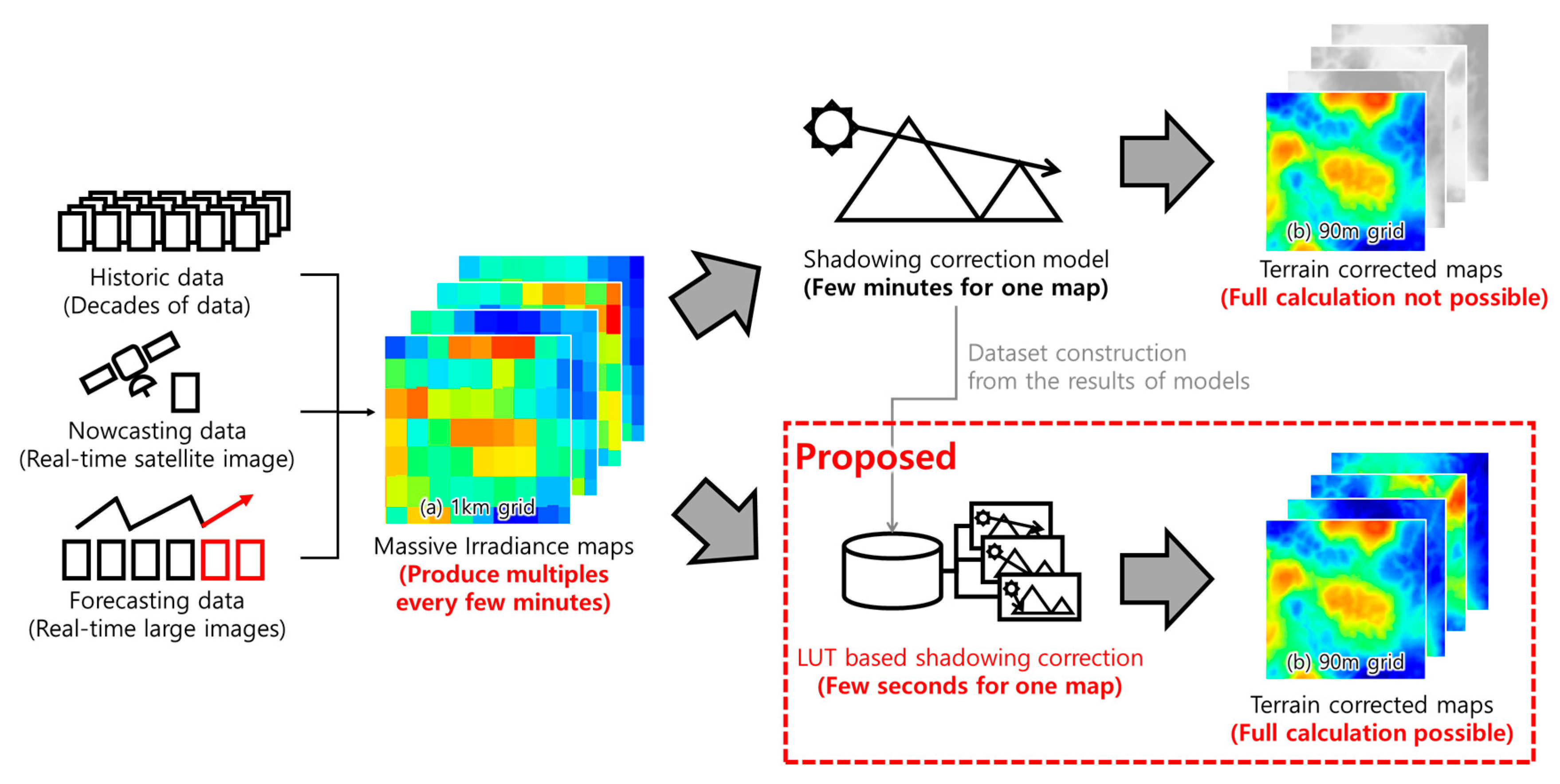
:1. Introduction
2. Materials and Methods
2.1. Data
2.1.1. Low-Resolution Solar Irradiance Maps
2.1.2. High-Resolution Terrain Maps
2.2. Shadow Calculation Algorithms
2.2.1. Equations and Numerical Calculations
2.2.2. Regional Calculations
2.2.3. Calculation Process and Lookup Table
2.3. Proposed Real-Time Calculation Model
2.3.1. Lookup Table-Based Dataset Composition
2.3.2. Fast Interpolation Method
2.3.3. Memory Optimization
2.4. Methodology
2.4.1. Terrain Correction Verification
2.4.2. Memory Analysis
2.4.3. Calculation Time Analysis
3. Results
3.1. Terrain Correction
3.2. Required Memory and Optimization
3.3. Calculation Time
4. Discussion
4.1. Application of Fast Terrain Correction
4.2. Influence of Terrain Correction
4.3. Accuracy of the Model
5. Conclusions
Author Contributions
Funding
Data Availability Statement
Conflicts of Interest
References
- Kim, C.K.; Kim, H.G.; Kang, Y.H.; Yun, C.Y.; Lee, Y.G. Intercomparison of satellite-derived solar irradiance from the GEO-KOMSAT-2A and HIMAWARI-8/9 satellites by the evaluation with ground observations. Remote Sens. 2020, 12, 2149. [Google Scholar] [CrossRef]
- Huang, G.; Li, Z.; Li, X.; Liang, S.; Yang, K.; Wang, D.; Zhang, Y. Estimating surface solar irradiance from satellites: Past, present, and future perspectives. Remote Sens. Environ. 2019, 233, 111371. [Google Scholar] [CrossRef]
- Perez, R.; Ineichen, P.; Moore, K.; Kmiecik, M.; Chain, C.; George, R.; Vignola, F. A new operational model for satellite-derived irradiances: Description and validation. Sol. Energy 2002, 73, 307–317. [Google Scholar] [CrossRef] [Green Version]
- Dubayah, R.; Rich, P.M. Topographic Solar-Radiation Models for Gis. Int. J. Geogr. Inf. Sci. 1995, 9, 405–419. [Google Scholar] [CrossRef]
- Corripio, J.G. Vectorial algebra algorithms for calculating terrain parameters from dems and solar radiation modelling in mountainous terrain. Int. J. Geogr. Inf. Sci. 2003, 17, 1–23. [Google Scholar] [CrossRef]
- Bosch, J.L.; Batlles, F.J.; Zarzalejo, L.F.; López, G. Solar resources estimation combining digital terrain models and satellite images techniques. Renew. Energy 2010, 35, 2853–2861. [Google Scholar] [CrossRef]
- Ruiz-Arias, J.A.; Cebecauer, T.; Tovar-Pescador, J.; Šúri, M. Spatial disaggregation of satellite-derived irradiance using a high-resolution digital elevation model. Sol. Energy 2010, 84, 1644–1657. [Google Scholar] [CrossRef]
- Zhang, S.; Li, X.; She, J.; Peng, X. Assimilating remote sensing data into GIS-based all sky solar radiation modeling for mountain terrain. Remote Sens. Environ. 2019, 231, 111239. [Google Scholar] [CrossRef]
- Ma, Y.; He, T.; Liang, S.; Mcvicar, T.R.; Hao, D.; Liu, T.; Jiang, B. Estimation of fine spatial resolution all-sky surface net shortwave radiation over mountainous terrain from Landsat 8 and Sentinel-2 data. Remote Sens. Environ. 2023, 285, 113364. [Google Scholar] [CrossRef]
- Romero, L.F.; Tabik, S.; Vías, J.M.; Zapata, E.L. Fast clear-sky solar irradiation computation for very large digital elevation models. Comput. Phys. Commun. 2008, 178, 800–808. [Google Scholar] [CrossRef]
- Oh, M.; Park, H.D. A new algorithm using a pyramid dataset for calculating shadowing in solar potential mapping. Renew. Energy 2018, 126, 465–474. [Google Scholar] [CrossRef]
- Tabik, S.; Villegas, A.; Zapata, E.L.; Romero, L.F. A fast GIS-tool to compute the maximum solar energy on very large terrains. Procedia Comput. Sci. 2012, 9, 364–372. [Google Scholar] [CrossRef]
- Lukač, N.; Žalik, B. GPU-based roofs’ solar potential estimation using LiDAR data. Comput. Geosci. 2013, 52, 34–41. [Google Scholar] [CrossRef]
- Huang, Y.; Chen, Z.; Wu, B.; Chen, L.; Mao, W.; Zhao, F.; Wu, J.; Wu, J.; Yu, B. Estimating roof solar energy potential in the downtown area using a GPU-accelerated solar radiation model and airborne LiDAR data. Remote Sens. 2015, 7, 17212–17233. [Google Scholar] [CrossRef] [Green Version]
- Stendardo, N.; Desthieux, G.; Abdennadher, N.; Gallinelli, P. GPU-enabled shadow casting for solar potential estimation in large urban areas. Application to the solar cadaster of Greater Geneva. Appl. Sci. 2020, 10, 5361. [Google Scholar] [CrossRef]
- Geraldi, E.; Larosa, S.; Romano, F.; Cersosimo, A.; Cimini, D.; Di Paola, F.; Gallucci, D.; Gentile, S.; Nilo, S.T.; Ricciardelli, E.; et al. The analysis of static boundary condition in solar resource assessment by satellite: The role of high-resolution Digital Terrain Model in irradiance downscaling process. In Proceedings of the 4th International Conference on Energy & Meteorology (ICEM), Bari, Italy, 27–29 June 2017. [Google Scholar]
- Šúri, M.; Huld, T.A.; Dunlop, E.D. PV-GIS: A web-based solar radiation database for the calculation of PV potential in Europe. Int. J. Sustain. Energy 2005, 24, 55–67. [Google Scholar] [CrossRef]
- Suri, M.; Cebecauer, T. SolarGIS: New Web Based Service Offering Solar Radiation Data and Tools for Europe, North Africa and Middle East; International Solar Energy Society: Freiburg im Breisgau, Germany, 2016; pp. 1–7. [Google Scholar]
- Calcabrini, A.; Ziar, H.; Isabella, O.; Zeman, M. A simplified skyline-based method for estimating the annual solar energy potential in urban environments. Nat. Energy 2019, 4, 206–215. [Google Scholar] [CrossRef] [Green Version]
- Vartholomaios, A. A machine learning approach to modelling solar irradiation of urban and terrain 3D models. Comput. Environ. Urban Syst. 2019, 78, 101387. [Google Scholar] [CrossRef]
- Lin, S.; Chen, N.; Zhou, Q.; Lin, T.; Li, H. A Scheme for Quickly Simulating Extraterrestrial Solar Radiation over Complex Terrain on a Large Spatial-Temporal Span—A Case Study over the Entirety of China. Remote Sens. 2022, 14, 1753. [Google Scholar] [CrossRef]
- Şen, Z.; Şahin, A.D. Spatial interpolation and estimation of solar irradiation by cumulative semivariograms. Sol. Energy 2001, 71, 11–21. [Google Scholar] [CrossRef]
- Chelbi, M.; Gagnon, Y.; Waewsak, J. Solar radiation mapping using sunshine duration-based models and interpolation techniques: Application to Tunisia. Energy Convers. Manag. 2015, 101, 203–215. [Google Scholar] [CrossRef]
- Leirvik, T.; Yuan, M. A Machine Learning Technique for Spatial Interpolation of Solar Radiation Observations. Earth Space Sci. 2021, 8, 1–22. [Google Scholar] [CrossRef]
- Kim, C.K.; Kim, H.G.; Kang, Y.H.; Yun, C.Y. Toward Improved Solar Irradiance Forecasts: Comparison of the Global Horizontal Irradiances Derived from the COMS Satellite Imagery Over the Korean Peninsula. Pure Appl. Geophys. 2017, 174, 2773–2792. [Google Scholar] [CrossRef]
- Dozier, J. Rapid Calculation of Terin Parameters for Radiation Modeling From Digital Elevation Data. IEEE Trans. Geosci. Remote Sens. 1990, 28, 963–969. [Google Scholar] [CrossRef]
- Fu, P.; Rich, P. Design and implementation of the Solar Analyst: An ArcView extension for modeling solar radiation at landscape scales. In Proceedings of the 19th Annual ESRI User Conference, San Diego, CA, USA, 26–30 July 1999. [Google Scholar]
- Perez, R.; Ineichen, P.; Seals, R.; Michalsky, J.; Stewart, R. Modeling daylight availability and irradiance components from direct and global irradiance. Sol. Energy 1990, 44, 271–289. [Google Scholar] [CrossRef] [Green Version]
- Palz, W.; Page, J.; Flynn, R.; Dogniaux, R.; Preuveneers, G.; Palz, W. European Solar Radiation Atlas. Volume II, Global and Diffuse Radiation on Vertical and Inclined Surfaces; Palz, W., Ed.; Verlag TÜV Rheinland GmbH: Köln, Germany, 1996. [Google Scholar]
- Freitas, S.; Catita, C.; Redweik, P.; Brito, M.C. Modelling solar potential in the urban environment: State-of-the-art review. Renew. Sustain. Energy Rev. 2015, 41, 915–931. [Google Scholar] [CrossRef]
- SciPy Documentation. Available online: https://docs.scipy.org/doc/scipy/ (accessed on 9 February 2022).
- Oh, M.; Park, H.D. Optimization of solar panel orientation considering temporal volatility and scenario-based photovoltaic potential: A case study in Seoul National University. Energies 2019, 12, 3262. [Google Scholar] [CrossRef] [Green Version]
- Yu, W.; Patros, P.; Young, B.; Klinac, E.; Walmsley, T.G. Energy digital twin technology for industrial energy management: Classification, challenges and future. Renew. Sustain. Energy Rev. 2022, 161, 112407. [Google Scholar] [CrossRef]
- Deng, T.; Zhang, K.; Shen, Z.J. (Max) A systematic review of a digital twin city: A new pattern of urban governance toward smart cities. J. Manag. Sci. Eng. 2021, 6, 125–134. [Google Scholar] [CrossRef]
- Francisco, A.; Mohammadi, N.; Taylor, J.E. Smart City Digital Twin-Enabled Energy Management: Toward Real-Time Urban Building Energy Benchmarking. J. Manag. Eng. 2020, 36, 04019045. [Google Scholar] [CrossRef]
- Kakimoto, M.; Endoh, Y.; Shin, H.; Ikeda, R.; Kusaka, H. Probabilistic Solar Irradiance Forecasting by Conditioning Joint Probability Method and Its Application to Electric Power Trading. IEEE Trans. Sustain. Energy 2019, 10, 983–993. [Google Scholar] [CrossRef]
- Libra, M.; Mrázek, D.; Tyukhov, I.; Severová, L.; Poulek, V.; Mach, J.; Šubrt, T.; Beránek, V.; Svoboda, R.; Sedláček, J. Reduced real lifetime of PV panels—Economic consequences. Sol. Energy 2023, 259, 229–234. [Google Scholar] [CrossRef]


| Algorithm Category | Required Calculations | Changes According to the Sun’s Position | Examples | Each Calculation Time |
|---|---|---|---|---|
| Static | Once | X | SVF, DHI ratio, etc. | High |
| Dynamic | Every case | O | Shadows, DNI ratio, etc. | Relatively low |
| Calculation Method | Direct (Beam) Irradiance Shadowing | Diffuse Irradiance Shadowing | Point Calculation | Regional Calculation | Required Memory |
|---|---|---|---|---|---|
| Equation | Fast | Difficult | Fast | Very difficult | Low |
| Numerical | Fast | Slow | Fast | Very slow | Medium |
| Lookup table | Fast | Fast | Fast | Fast | High |
| Calculation Time for One Satellite-Based Solar Map (s) | Calculation Time for Processing 1 Year of Past Data with 15 Min Intervals (h) | |
|---|---|---|
| GRASS GIS r.horizon | 70,000 (20 h) | 400,000 (43 years) |
| VIEWMAP with the pyramid dataset | 4000 (1 h) | 20,000 (2 years) |
| LUT-based dataset | 40 | 210 |
| LUT DB + Fast interpolation model | 6 | 32 |
Disclaimer/Publisher’s Note: The statements, opinions and data contained in all publications are solely those of the individual author(s) and contributor(s) and not of MDPI and/or the editor(s). MDPI and/or the editor(s) disclaim responsibility for any injury to people or property resulting from any ideas, methods, instructions or products referred to in the content. |
© 2023 by the authors. Licensee MDPI, Basel, Switzerland. This article is an open access article distributed under the terms and conditions of the Creative Commons Attribution (CC BY) license (https://creativecommons.org/licenses/by/4.0/).
Share and Cite
Oh, M.; Kim, C.K.; Kim, B.; Kang, Y.; Kim, H.-G. Real-Time Terrain Correction of Satellite Imagery-Based Solar Irradiance Maps Using Precomputed Data and Memory Optimization. Remote Sens. 2023, 15, 3965. https://0-doi-org.brum.beds.ac.uk/10.3390/rs15163965
Oh M, Kim CK, Kim B, Kang Y, Kim H-G. Real-Time Terrain Correction of Satellite Imagery-Based Solar Irradiance Maps Using Precomputed Data and Memory Optimization. Remote Sensing. 2023; 15(16):3965. https://0-doi-org.brum.beds.ac.uk/10.3390/rs15163965
Chicago/Turabian StyleOh, Myeongchan, Chang Ki Kim, Boyoung Kim, Yongheack Kang, and Hyun-Goo Kim. 2023. "Real-Time Terrain Correction of Satellite Imagery-Based Solar Irradiance Maps Using Precomputed Data and Memory Optimization" Remote Sensing 15, no. 16: 3965. https://0-doi-org.brum.beds.ac.uk/10.3390/rs15163965