
Spatial Statistical Prediction of Solar-Induced Chlorophyll Fluorescence (SIF) from Multivariate OCO-2 Data

School of Mathematics and Applied Statistics, University of Wollongong, Wollongong, NSW 2522, Australia
*
Author to whom correspondence should be addressed.
Remote Sens. 2023, 15(16), 4038; https://0-doi-org.brum.beds.ac.uk/10.3390/rs15164038
Submission received: 30 June 2023
/
Revised: 2 August 2023
/
Accepted: 8 August 2023
/
Published: 15 August 2023
(This article belongs to the Special Issue Spatial and Spatio-Temporal Statistics: Methods and Applications in Remote Sensing)
Abstract
:Solar-induced chlorophyll fluorescence, or SIF, is a part of the natural process of photosynthesis. SIF can be measured from space by instruments such as the Orbiting Carbon Observatory-2 (OCO-2), making it a useful proxy for monitoring gross primary production (GPP), which is a critical component of Earth’s carbon cycle. The complex physical relationship between SIF and GPP is frequently studied using OCO-2 observations of SIF since they offer the finest spatial resolution available. However, measurement error (noise) and large gaps in spatial coverage limit the use of OCO-2 SIF to highly aggregated scales. To study the relationship between SIF and GPP across varying spatial scales, de-noised and gap-filled (i.e., Level 3) SIF data products are needed. Using a geostatistical methodology called cokriging, which includes kriging as a special case, we develop coSIF: a Level 3 SIF data product at a 0.05-degree resolution. As a natural secondary variable for cokriging, OCO-2 observes column-averaged atmospheric carbon dioxide concentrations (XCO) simultaneously with SIF. There is a suggested lagged spatio-temporal dependence between SIF and XCO, which we characterize through spatial covariance and cross-covariance functions. Our approach is highly parallelizable and accounts for non-stationary measurement errors in the observations. Importantly, each datum in the resulting coSIF data product is accompanied by a measure of uncertainty. Extant approaches do not provide formal uncertainty quantification, nor do they leverage the cross-dependence with XCO.
1. Introduction
Quantifying the spatio-temporal patterns of gross primary production (GPP), which is the total amount of carbon dioxide (CO) absorbed through photosynthesis, is an important aspect of studying ecosystem function and the carbon cycle. While GPP cannot be directly measured on global scales, remote sensing observations of solar-induced chlorophyll fluorescence (SIF) provide a reliable proxy for quantifying GPP globally [1,2,3,4]. SIF occurs when chlorophyll molecules return from excited to non-excited states and dissipate the light energy absorbed during photosynthesis, in part, through re-emission of fluorescent photons in the spectral range between 650 nm (red) and 800 nm (far red) with varying intensity [5]. Hence, there is a complex physical relationship between SIF and GPP [6]. An accurate characterization of this relationship relies on the availability of high-quality, spatially complete SIF data [7].
Measurements of SIF have been examined in laboratory and field studies, from the sub-cellular scale up to the leaf scale, for decades [8], although more recently it has become possible to measure SIF from satellite instruments at the global scale [9,10,11,12]. Different satellites collect global remote-sensing observations of SIF at different spatial and temporal resolutions. Available records of these observations, sometimes called Level 2 data products (e.g., [13]), are of limited use in analyzing the physical relationship with GPP due to large measurement errors, coarse spatial resolutions, and/or sparse spatial observations [14]. These issues are less prevalent in the fine-resolution, high-density observations recently available from the Tropospheric Monitoring Instrument (TROPOMI), but gaps in coverage are still present [15,16]. To examine the relationship between SIF and GPP across different spatial scales, de-noised and gap-filled (i.e., Level 3) data products with quantified uncertainties are required.
Several studies have proposed methods to produce Level 3 SIF data products with enhanced spatial resolution, typically at 0.05 degrees and as fine as 500 m in longitude and latitude. These methods are based on a variety of Level 2 SIF data products, but they are categorized into two general approaches: (1) physiologically motivated approaches that leverage relationships between SIF and other explanatory variables to downscale SIF from coarser resolutions [17,18,19,20,21], and (2) machine learning approaches that either downscale coarse-resolution SIF using ancillary datasets available at a finer resolution [22,23,24], or gap-fill fine-resolution but spatially sparse SIF observations [25,26,27]. Though these Level 3 data products have demonstrated overall capability in capturing the spatial patterns in SIF [7], none are accompanied by formally quantified uncertainties of each gap-filled SIF value. As a consequence, validation procedures for estimated Level 3 SIF fields are lacking.
Spatial statistical prediction (e.g., kriging) is another approach for producing Level 3 data products. As highlighted by [28], a key advantage of a statistical approach is the full quantification of uncertainty that is immediately available with the spatial predictions. Locally constructed kriging models were developed in [29,30] to produce coarse-resolution Level 3 data products for multiple remotely sensed processes, including SIF. However, a problematic feature of local kriging is that the spatial union of multiple local models can result in an incoherent global probability structure and, hence, in invalid prediction uncertainties [28]. Instead, spatial-statistical methods that consider satellite observations as realizations from an underlying spatial stochastic process that covers the domain of interest result in coherent uncertainty quantifications of all upscaled SIF estimates.
When observations of multivariate processes are available, as is often the case in remote sensing, the additional information can be leveraged for prediction of a primary process of interest through cokriging [31,32]. For instance, NASA’s Orbiting Carbon Observatory-2 (OCO-2) satellite observes both SIF and column-averaged atmospheric carbon dioxide concentrations (XCO). Since CO is a reactant in the process of photosynthesis, for which SIF is a proxy, dependence between SIF and XCO is expected.
In this article, we propose a cokriging-based method that leverages any dependence between SIF and XCO to produce de-noised and gap-filled predictions for SIF with quantified uncertainties. This reduces to a kriging-based method when SIF has no dependence on XCO, which can happen during non-productive seasons. Our cokriging method is highly parallelizable, directly accounts for non-stationary measurement errors, and offers flexible spatial resolution through aggregation of the fine-resolution Level 3 data product. Here, we apply the cokriging method to multivariate OCO-2 data over a large region in North America to illustrate coSIF, which is our 0.05-degree, monthly resolution Level 3 SIF data product that includes coherent uncertainty quantification of each SIF estimate. Compared to kriging with SIF observations only, we find that our cokriging method can reduce prediction uncertainty and improve prediction accuracy when there is dependence between SIF and XCO.
The remainder of this article is organized as follows. In Section 2, we describe how OCO-2 observations of SIF and XCO are used in the construction of a bivariate spatial-statistical model, and how this model is used to produce cokriging predictions with their uncertainties quantified. Validation strategies are described in Section 2.5, and in Section 3 the strategies are applied to the coSIF data product. We give conclusions and discuss future research directions in Section 4.
2. Materials and Methods
Our multivariate spatial-statistical-prediction framework involves four major steps: (1) Obtain multivariate, monthly remote sensing datasets that are spatially indexed (Section 2.1 and Section 2.2). (2) Use the multivariate spatial data to estimate covariance and cross-covariance functions of a multivariate spatial-statistical model (Section 2.3). (3) Use the multivariate spatial (cross-) covariance functions to predict the process of interest along with uncertainties (root-mean-squared prediction errors) on a fine-resolution () regular grid (Section 2.4). (4) Evaluate the predictions and their uncertainties using a variety of statistical validation metrics (Section 2.5). When applied to SIF and XCO, we obtain an estimated, de-noised, gap-filled SIF data product, coSIF, which includes uncertainty quantification. These methods and the specific datasets used to create coSIF are detailed in the following subsections.
2.1. Datasets Used
Production of the coSIF data product requires both observational and auxiliary datasets.
- Observational Datasets: OCO-2 SIF and XCO
OCO-2 is a NASA satellite that launched in July 2014 and actively observes two main quantities: SIF and XCO [3,33]. Currently, OCO-2 yields the finest spatial resolution of all spaceborne SIF observations [13], and it is often used as a benchmark for the validation of SIF data products (e.g., [14,20,24]). The OCO-2 satellite has a sun-synchronous, 98.8-min polar orbit with roughly a 13:36 local crossing time and a 16-day ground-track repeat cycle [34]. Observations are made in one of three modes: “nadir”, “glint”, and “target”. In nadir mode, the viewing zenith angle (VZA) is near zero, and the instrument views the ground directly beneath the satellite, while the glint mode generally has higher VZAs as it tracks high reflectance from Earth’s surface. Target mode has VZAs that can vary substantially, since various locations on Earth’s surface are targeted when in this mode. Each mode operates at a fine spatial resolution; for example, swath widths are approximately 10 km with eight measurements across the track, each about 1.3 km × 2.25 km (across × along track) in nadir mode [33].
For use among the broader scientific community, NASA publishes OCO-2 datasets as collections of “Lite” files. Lite files contain bias-corrected, daily Level 2 (non-gridded) data at the same spatio-temporal resolution as that of the original observations. We obtained version 10r Lite files for SIF [35] and XCO [36], which are available through NASA’s Goddard Earth Sciences Data and Information Services Center (GES DISC), each from September 2014 to February 2022 inclusive. SIF measurements are retrieved in Watts per square meter, per steradian, and per micrometer (hereafter W m srm) at wavelengths of 757 nm and 771 nm. From these wavelengths, estimates of SIF are produced at a wavelength of 740 nm. As recommended in [13], we use the SIF estimates at 740 nm, which have a lower error overall than the measurements at the 757 nm and 771 nm wavelengths [3]. Further, we only retain observations associated with quality flags 0 and 1 for the Level 2 SIF data. With regard to the Level 2 XCO data, which are available in parts per million (ppm), we only retain those associated with quality flag 0. Estimates of measurement error standard deviations accompany both the SIF measurements and the XCO measurements; we square these measurement error standard deviations to obtain the corresponding measurement error variances.
- Auxiliary Dataset: MODIS LCC
From 2001, the Terra and Aqua combined Moderate Resolution Imaging Spectroradiometer (MODIS) Land Cover Climate Modeling Grid (MCD12C1) provides yearly land-cover classification (LCC) at a 0.05-degree spatial resolution over the globe. We obtained MCD12C1 Version 6.1 [37] for 2021 to produce a binary mask of land-based prediction locations. Following the International Geosphere-Biosphere Programme (IGBP) classification scheme, we use values not marked as “water” to create the land mask over North America.
2.2. Data Preparation
We first group the daily, spatially irregular SIF and XCO measurements and their corresponding measurement error variances by month and average both the measurements and the measurement error variances onto a regular grid with a 0.05-degree spatial resolution (around 5.6 km × 5.6 km at the Equator), which aligns with the MODIS Climate Modeling Grid. This resolution is the same order of magnitude as that of the OCO-2 footprint and, by averaging multiple measurements, we effectively reduce the measurement error at this resolution [1]. For illustration purposes, we restrict the gridded data used in our analysis to a large region over North America within latitude and longitude boundaries of 22 to 58 degrees North and −125 to −65 degrees East, respectively. This region, which includes the conterminous United States, is similar to that considered by [24], and features heterogeneous land-cover types over which to evaluate the coSIF data product.
As an indicator of photosynthetic activity, SIF is expected to exhibit an inverse relationship with XCO. Indeed, the monthly time series in Figure 1 show that SIF and XCO follow strong seasonal patterns that are shifted relative to one another, with the annual maxima in SIF occurring about one month before the annual minima in XCO. To leverage this dependence, we use both SIF data and XCO data one month ahead in a multivariate spatial statistical model. We present our results for four months in 2021 to represent the four seasons in North America. For SIF, we use February, April, July, and October 2021, and hence we group these with the XCO data from March, May, August, and November 2021, respectively. For each pair of months, the columns of Figure 2 offer histograms of the OCO-2 data at a 0.05-degree resolution, along with the number of data points available in each month. As in Figure 1, Figure 2 shows that larger XCO values follow months in which SIF values are small, and that XCO decreases after months in which SIF values are larger. Additionally, Figure 2 shows that there is more variability in the summer months: July (SIF) and August (XCO). This variability is due to increased SIF activity in certain productive regions, which in turn leads to additional spatial variability in XCO. Figure 3 shows the spatial distribution of the OCO-2 data at a 0.05-degree resolution for the summer months. Notice the spatial variability in both SIF and XCO, as well as the large gaps where there are no data.
2.3. Modeling Multivariate Spatial Dependence between SIF and XCO
In what follows, we discuss the modeling approach for a single pair of months (e.g., SIF in July and XCO in August). Let D be the spatial region of interest shown in Figure 3 and described in Section 2.2, tessellated by 0.05-degree-resolution grid cells. Then, refers to the centroid of a grid cell in D. The true SIF process averaged over a given month is , and the true XCO process averaged over the following month is , but the OCO-2 satellite observations are imperfect and incomplete on D. We denote the gridded and monthly averaged SIF and XCO data (subsequently simply referred to as “data”) by the vectors and , respectively, with , , where there are grid cells that contain SIF data and grid cells that contain XCO data. In Figure 3 (Top), , and in Figure 3 (Bottom), ; see also Figure 2. In the spatial domain D, we model the noisy data value at grid cell location as
where is a set of (non-stationary) independent measurement errors, with mean zero and variances obtained from the Lite files and averaged as described in Section 2.2. The latent processes and are defined on all and are modeled as
Here, represents the deterministic trend component, which can be thought of as large-scale variation, while is a random process with zero mean that accounts for any remaining spatial variation. For , we write
where is a mean-zero Gaussian process that captures the smooth small-scale variation, and is a process uncorrelated at the grid scale with mean zero and constant variance that accounts for micro-scale variation.
Because our objective is spatial prediction, we take a relatively parsimonious approach for modeling to avoid over-fitting the data. At each location , estimates for the deterministic trend components, , , are obtained through regression on a vector of covariates, , as follows:
where is a vector of ordinary-least-squares-estimated regression coefficients obtained from fitting to separately for . For each , the elements of include an intercept term, and spatial bisquare basis functions (e.g., [38]), here used to express a spatial trend. We obtained the bisquare basis functions from the package FRK in R [39] and chose them such that their spatial supports cover the data region with centers arranged in a regular, grid. Some basis functions over water were not appropriate for the land-based SIF data; three were identified and withheld from , the vector of covariates for SIF. Hence, and . The locations of the basis functions and the extent of their spatial supports are displayed in Figure 4.
After the estimated spatial trend is removed, the behavior of the small-scale spatial variation is modeled based on the vectors of spatial residuals , with elements computed from the data as
To mitigate bias and trend contamination often found in the residuals ([40], Section 2.2.5), we standardize each set of values using the empirical mean, , and standard deviation, , as follows:
, and . We then model the standardized spatial residuals as
where is the smooth small-scale variation and is the micro-scale variation with mean zero and variance on the standardized scale for the standardized residuals , and are spatially varying independent measurement errors on the standardized scale, obtained from the spatially varying independent measurement errors as defined for Equation (1).
The smooth small-scale-variation processes (for SIF) and (for XCO) are the focus of our multivariate spatial modeling efforts. Between any two spatial locations , we model the underlying spatial dependence and cross-dependence in the standardized small-scale-variation processes with a bivariate covariance function , for . For , we selected the full bivariate Matérn model [41,42], popular for its flexible parameterization of spatial smoothness. For spatial lag , the model is symmetric and isotropic:
for , where is a scale parameter and is a (cross-) correlation coefficient, with when and otherwise. The function is the Matérn correlation function [43,44], with and denoting the smoothness and correlation length, respectively. Further, is the gamma function and is a modified Bessel function of the second kind of order ([45], Section 10.2). As detailed in [41], the values of , , and that result in a positive-semidefinite bivariate covariance function belong to a constrained parameter space. Finally, note that since and are locations on Earth’s surface, we avoid Euclidean distance and let be the chordal distance between and (e.g., [46]).
To estimate the parameters of the full bivariate Matérn covariance model, we use the standardized residuals, , , given by Equation (6). We first compute empirical semivariograms and cross-semivariograms, and then we fit the parameters of the covariance and cross-covariance functions simultaneously using a multivariate extension of the weighted-least-squares approach developed in [47]. This process is described in Appendix A.1; a check for the validity of the fitted parameters is also established there.
2.4. Generating the Spatially Contiguous coSIF Data Product with Quantified Uncertainties Based on Cokriging
From the noisy and relatively sparse spatial data (SIF) and (XCO), we seek the optimal spatial prediction, , and its root-mean-squared prediction error, , for the latent SIF process, , at each of the 0.05-degree land-based grid cell locations , , in the domain D spanning North America, shown in Figure 3. In generating our SIF data product, we produce spatial predictions at the 0.05-degree resolution for two main reasons: (1) 0.05 degrees is emerging as the standard for Level 3 SIF data products (e.g., [20,23,25,26,27]); (2) predictions are at the same resolution as the pre-processed data (Section 2.2). Since the spatial covariance model is formulated at the 0.05-degree resolution, upscaling to coarser resolutions is straightforward (e.g., [48]).
The practice of leveraging interdependence between multiple related processes to optimally predict one of those processes is known in geostatistics as cokriging (e.g., [32]). Recall from Equation (2) that we model the spatial process as the combination of large-scale variation and any remaining spatial variation through the decomposition , for . Having standardized the SIF and XCO data as in Equation (6), our task in cokriging is to optimally predict , which is the standardized version of defined in Equation (3). From predictions of , we can obtain predictions of on the original scale by reversing the standardization with a simple linear transformation.
As in Section 2.3, information about the behavior of (for SIF) and (for XCO) is taken from the standardized spatial residuals and described in Equation (6). For a given set of months, and have a combined size on the order of 50,000 elements (see Figure 2), so that traditional cokriging is computationally intractable due to a required matrix inversion that is shown in Equation (11) below. However, spatial prediction is a relatively local operation ([40], Section 3.4), so for a given prediction location , we use a local neighborhood defined by the 150 values whose corresponding locations are closest in chordal distance to , respectively, in and . Let and be these 150-dimensional vectors of local residuals, and define . The bivariate spatial variation across the locations associated with and , , is described by the variance-covariance matrix,
where each block is a 150 × 150 (cross-) covariance matrix having elements given by from Equation (8) with estimated parameters substituted in; is the 150 × 150 identity matrix; and has elements from the definition of in Equation (7), corresponding to locations associated with . Similarly, we obtain the covariance vector , with elements of the j-th sub-vector () given by , where
; is the spatial location associated with ; denotes chordal distance; and is the indicator function. Notice the absence of measurement error variances in Equation (10), since we are predicting the (noiseless) residual process.
Then, by minimizing the mean squared prediction error (MSPE) over all linear predictors of given , we obtain the cokriging prediction and minimized MSPE (Equations (6) and (7) in [32])):
The estimator given in Equation (11) is an unbiased linear predictor for under squared error loss, and the uncertainty measure we use is the square root of the MSPE given in Equation (12); notice that is an approximation to the optimal predictor, , since it is based on a subset of the available data. To obtain predictions and uncertainty quantification on the original scale of the latent SIF process, we reverse the standardization to yield
Operationally, these predictions and their root-mean-squared prediction errors, given by Equations (13) and (14), respectively, can be produced at each location in a highly parallelizable manner. Hence, for each month, our 0.05-degree resolution coSIF data product consists of and .
2.5. Statistical Validation of the coSIF Data Product
Cross-validation is a widely used method for evaluating the predictive performance of statistical models [49]. The method seeks to evaluate model predictions by withholding some subset of the available data when fitting the model and making predictions, using the withheld subset for validation, and repeating with other subsets. Often, one does leave-one-out cross-validation, where data are withheld one at a time, or K-fold cross-validation, where data are withheld in “folds”. However, there are two important considerations in the spatial setting. First, fitting multiple spatial models to different subsets of data can quickly become computationally prohibitive if the number of subsets is large. Second, the spatial arrangement of the withheld validation data is important. For example, the locations of the withheld data may be chosen at random, or they may be chosen so that a region or block of data are missing. The latter reflects a common scenario in remote-sensing applications where a satellite’s observations are hindered by blocks of clouds or retrieval malfunctions. In a spatial context, missing blocks of data also lead to a more rigorous validation test, since spatial prediction over large spans of unobserved regions is generally a harder problem than that over small unobserved regions [50].
Given the challenges of cross-validation in the spatial setting, we instead evaluate the performance of geostatistical methods (cokriging and kriging) for producing our data product through validation (rather than cross-validation) within blocks of withheld SIF data. Specifically, for a given block with spatial support A, the SIF validation data associated with spatial locations are withheld from the available data, leaving , of dimension , for use in the prediction framework. Because the withheld validation data, , contain measurement error, we seek to predict rather than the noiseless latent vector in the validation setting [28]. It is easy to see that the predicted values, , are identical to given by Equation (13). However, the RMSPEs of the elements of are different from those of . Specifically,
To assess the advantage of leveraging geostatistical dependence between SIF and XCO, we use both a cokriging and a kriging version of this procedure to produce predictions of the withheld data. To assess the advantage of incorporating spatial dependence within SIF in the cokriging and kriging models, we compare the validation predictions from these geostatistical models to those from a trend-surface-only model (a special case of kriging) that does not leverage spatial dependence. Kriging and trend-surface predictions are based on SIF data alone, whereas cokriging predictions are based on SIF and XCO data. Further details are given in Appendix A.2.
We select a number of criteria to evaluate these predictions at validation locations. To characterize the marginal accuracy of the predictions, we consider average prediction error, or bias (BIAS), and root-average-squared prediction error (RASPE), given by
A benefit of a geostatistical prediction framework is that, at each prediction location , we obtain a predictive distribution, say , rather than a predicted value alone. Because we assume the data are Gaussian, each is a Gaussian distribution with mean and variance ; see Equations (13) and (15), respectively. Recall that the approximations are due to the predictor using only the nearest 150 data points for SIF and for XCO, and that the 150 data points for SIF are outside of the validation block A.
Through the predictive distribution, , we can quantify the uncertainty in our Level 3 coSIF data product. We compare these quantified uncertainties to analogous ones obtained from the univariate kriging model and the trend-surface-only model using scoring rules, which measure how well a probabilistic prediction aligns with what is actually observed. Here, we consider the interval score which assesses calibration and sharpness by favoring narrow prediction intervals and penalizing those that do not contain the true observation. With a two-sided prediction interval given by for at validation location , the interval score (INT) is given by
for , where and is the indicator function [51]. Another scoring rule that assesses both the first and second moments of a predictive distribution is the Dawid-Sebastiani score (DSS; [52]) defined as
for , where recall that is a distribution with mean and variance . Because is Gaussian, Equation (19) is functionally equivalent to the logarithmic score, which is one of the most-used proper scoring rules [53]. The INT and DSS are computed pointwise, for each validation location, and typically the average of each collection of scores is used to compare the different prediction frameworks, without any regard to the spatial dependence between them.
The validation summaries introduced above focus on an average of pointwise predictions, but since the predictions are spatially correlated within a given block A, it is also important to consider multivariate scoring rules. These scoring rules assess as a single multivariate prediction of through the corresponding multivariate predictive distribution denoted as . Again, because the process model in Equation (2) is Gaussian, is a multivariate Gaussian distribution with conditional mean vector and conditional variance-covariance matrix . Hence, can be assessed using the multivariate DSS:
The MDSS provides a scoring metric to assess multivariate predictive distributions (e.g., [51], Equation (25)). Our evaluation of Equation (20) in Section 3.3 uses to approximate , and we obtain an approximation of the diagonal elements of , which are needed for the pointwise scores, from the square of Equation (15). The whole variance-covariance matrix is approximated in Appendix A.3.
3. Results and Discussion
In this section, we provide an overview of our coSIF data product by considering a large region over North America that is within the latitude and longitude boundaries of 22 to 58 degrees North and −125 to −65 degrees East, respectively. We illustrate coSIF for North America in this article, but our framework applies equally to other large continental regions, albeit with different estimates of spatial dependence parameters. In Section 3.1, we present fitted bivariate spatial dependence models for February, April, July, and October 2021 (representing the four seasons), and we find strong spatial cross-dependence between SIF and XCO in July, the month with the most prominent SIF activity. In Section 3.2, we consider the spatial and seasonal patterns of the coSIF-derived predictions and their corresponding prediction uncertainties, with a focus on July 2021. Section 3.3 presents validation metrics for July 2021 where bivariate cokriging, univariate kriging, and trend-surface-only predictions of SIF are compared.
We produce all results on a high-end server with 56 physical cores and 376 gigabytes of memory. For reference, compute times using this architecture are as follows. Fitting the bivariate spatial model takes roughly 10 min for each pair of months. Production of the coSIF data product takes on the order of 12 h for each pair of months; however, the procedure is highly parallelizable and this compute time could be reduced by using multiple servers. In a given validation block, procuring validation predictions and approximating their corresponding multivariate variance-covariance matrix (see Appendix A.3) takes 15 to 30 min, depending on the amount of data in the block.
3.1. Evaluation of Fitted Spatial Models
Recall from Section 2.2 that we consider bivariate spatial models for SIF and XCO (with XCO one month ahead of SIF) for four months in 2021 to represent the four seasons in North America. These models are constructed for SIF in February, April, July, and October 2021, and grouped with the secondary variable XCO in March, May, August, and November 2021. Figure 5 shows the empirical and fitted (cross-) semivariogram models based on the standardized spatial residuals and , for each of the four months; the fitted model parameters for all four months are available in the Supplementary Material.
In Figure 5, the empirical semivariograms clearly indicate the presence of small-scale spatial dependence in SIF (and XCO) not captured by the basis function trend surface. The fitted semivariogram models exhibit relatively small correlation lengths (on the order of 50 to 100 km in all cases). In July 2021, the empirical cross-semivariogram indicates pronounced spatial cross-dependence between the small-scale SIF and XCO latent processes, and this is captured by the fitted cross-semivariogram model with cross-correlation coefficient, , and cross-correlation length, km. The smaller cross-correlation coefficients and/or cross-correlation lengths in the other three months considered suggest that the cross-dependence between SIF and XCO decreases when GPP, and hence SIF, is small. This suggests that when SIF activity is not prominent (e.g., when SIF values are small in Figure 1), it may be sufficient to de-noise and gap-fill SIF using the special case of kriging. Still, for many applications (e.g., agricultural planning and yield estimation), seasons of prominent SIF activity, such as the late spring and summer, are of primary interest. For months when SIF activity is prominent, we suggest operational decisions between cokriging and kriging be made based on the presence of dependence in the empirical cross-semivariogram for SIF and XCO. In what follows, we consider summer SIF activity through a focus on July 2021 where we have identified cross-dependence between SIF and XCO; results for the other three months shown in Figure 5 are provided in the Supplementary Material.
3.2. Level 3 coSIF Predictions and Quantified Uncertainties
Next, we consider the spatial characteristics of coSIF across D, the North American region of interest. Figure 6 shows the de-noised and gap-filled coSIF data product in July 2021, with SIF predictions given at a 0.05-degree resolution in the top panel, and the corresponding RMSPEs (i.e., prediction standard errors) in the bottom panel. The spatial predictions show that coSIF is prominent across the eastern half of the region, particularly in the North American Corn Belt, and less so across the western half of the region. The striped diagonal pattern of the prediction standard errors are representative of the OCO-2 orbit tracks (e.g., Figure 3). This is expected from the local behavior of cokriging, which leads to smaller prediction standard errors at grid locations in areas where the data are dense and larger prediction standard errors at grid locations where the data are sparse or non-existent.
The observed seasonal variation of SIF in Figure 1 is reproduced in the coSIF data product. When comparing Figure 6 to similar figures for different months (given in Figures S1–S3 in the Supplementary Material), coSIF predictions are lower in the spring (April), fall (October) and winter (February), and higher in the summer (July). This seasonal variation is also reflected in the prediction standard errors, which scale with the coSIF predictions; there is more variability in the residuals given by Equation (5) in the summer (July), so the prediction standard errors are larger. Still, for all months considered here, the coSIF RMSPEs are on average about four times smaller than the gridded measurement-error standard deviations obtained from the Level 2 Lite files as described for Equation (1) (see Table S1 in the Supplementary Material for uncertainty reduction estimates in all four months).
3.3. Validation of coSIF and Comparison with Simpler Methods
We evaluate the cokriging method for producing the coSIF data product by performing validation on data withheld in spatially contiguous blocks. As discussed in Section 2.3, the bivariate spatial covariance model used for cokriging is able to leverage cross-spatial dependence between SIF and XCO, beyond the spatial dependence within SIF alone. Hence, we perform the same validation procedure for the special case of kriging predictions of SIF (where no relationship between SIF and XCO is assumed). Prior to obtaining kriging predictions, we re-fit the univariate spatial covariance model for SIF using the SIF-only semivariogram. We also compare these geostatistical predictions to the special case of trend-surface-only predictions (where it is assumed further that there is no spatial dependence in the SIF residuals); see Appendix A.2.
As opposed to leave-one-out cross-validation, or K-fold cross-validation with subsets of validation data selected at random, validation with subsets of data missing in blocks is especially challenging in the geostatistical setting, since spatial predictions depend heavily on the quantity, proximity, and precision of nearby data. Here, we separately consider two 5-degree by 5-degree validation blocks outlined by the red squares in Figure 3. One of these blocks has extents [E, E, N, N] and covers a large section of Iowa in the center of the North American Corn Belt where SIF activity is especially prominent in July. The other block has extents [E, E, N, N] and consists predominately of cropland in the plains of Colorado and Kansas where SIF activity is more moderate in July. The spatial supports of these two validation blocks (Corn Belt and Cropland) are representative of large unobserved regions that realistically can occur in OCO-2 datasets (e.g., Figure 3).
Recall from Section 2.5 that we produce a prediction, , and prediction standard error, , at each validation location , for , in a given validation block with spatial support A where data are withheld from predictions. The validation standardized residuals are given by
As a diagnostic check, it is important to explore whether these residuals are standard-Gaussian distributed, which is an indicator that the model is a good fit to the data in our setting. Quantile-quantile (Q–Q) plots of validation standardized residuals in July 2021 are shown in Appendix B (Figure A1) for the two validation blocks. For both blocks, the Q–Q plots that result from using the cokriging, kriging, and trend-surface-only methods are all quite similar and show that the residuals are approximately Gaussian, although each set of residuals exhibits slightly heavy-tailed behavior relative to the standard Gaussian distribution. This initial diagnostic result indicates that more sensitive validation metrics are needed to distinguish between the different prediction methods.
We now evaluate the validation metrics outlined in Section 2.5 (BIAS, RASPE, INT, DSS, and MDSS). Table 1 presents these metrics for the validation predictions and prediction standard errors produced for July 2021 using the cokriging, kriging, and trend-surface-only methods in both validation blocks. With the exception of average prediction error (BIAS), which should be as close to zero as possible, all metrics are negatively oriented scores (lower is better). We find that BIAS is reasonably negligible for all methods in both validation blocks. The root-average-squared prediction error (RASPE) also exhibits similar results across the different prediction methods. The RASPE for cokriging and kriging is slightly lower than that for the trend-surface-only method, suggesting that leveraging the spatial dependence identified in Section 3.1 yields slightly improved prediction accuracy.
While prediction accuracy is important, prediction uncertainty must also be considered when performing probabilistic prediction. We summarize the distribution of our predictions using the average interval score (INT) and the average Dawid-Sebastiani score (DSS), which offer different assessments on the quality of the prediction uncertainties. Between the two validation blocks, INT differs slightly as follows: the 95% prediction intervals are best calibrated when using cokriging for the Corn Belt validation block and when using kriging for the Cropland validation block. However, cokriging is found to offer the best characterization of uncertainty with respect to DSS in both blocks. While cokriging and kriging are similar with respect to INT and DSS, the performance of the trend-surface-only method is noticeably worse.
In different ways, the BIAS, RASPE, INT, and DSS are all summary statistics of the validation standardized residuals given in Equation (21), averaged over all the residuals in the validation block. Thus, these metrics assess the individual predictive distributions at each validation location, and they weight each result equally. However, because spatial dependence is present in the residuals (see Figure A2 in Appendix B), we also consider a multivariate extension of the Dawid-Sebastiani score (MDSS) to evaluate the multivariate predictive distribution at all validation locations simultaneously. The MDSS metric clearly favors the methods that leverage spatial dependence (cokriging and kriging), which provide superior multivariate predictive distributions. Compared to kriging, cokriging achieves a slightly better MDSS in both validation blocks, suggesting there is an advantage to leveraging the dependence between SIF and XCO identified in Section 3.1.
The validation metrics presented in Table 1 suggest that proper characterization of uncertainty requires that the prediction method accounts for spatial dependence in the data. Cokriging and kriging both account for spatial dependence, but cokriging offers smaller prediction uncertainty when there is cross-dependence between SIF and XCO. The validation metrics in Table 1 are available for each of the other three months considered in this study in Tables S2–S4 in the Supplementary Material. There, we find that when there is weak dependence between SIF and XCO, there is little advantage in cokriging. Instead, modeling the univariate SIF covariance function and predicting using kriging is more efficient and provides comparable results to cokriging when there is weak dependence between SIF and XCO.
4. Conclusions, Limitations, and Future Research
Satellite observations of SIF provide a viable proxy for GPP at the global scale [3,6]. However, these observational data are noisy and spatially incomplete so scientists need de-noised and gap-filled Level 3 data products to better characterize the relationship between SIF and GPP. Here, we use a geostatistical methodology called cokriging to produce coSIF, a Level 3 SIF data product at a 0.05-degree, monthly resolution with uncertainty quantification. Our highly parallelizable approach leverages OCO-2 observations of both SIF and XCO, which we show helps to reduce the uncertainty of the Level 3 data product in months of high GPP. It achieves this by modeling the cross-dependence between SIF and XCO one month later and, moreover, it accounts for non-stationary measurement errors in the observations. Due to its fine resolution, coSIF can be aggregated to coarser resolutions, along with coherent uncertainty quantification, which enables statistical comparison with other SIF products at varying resolutions.
We limit our analysis of coSIF to a large region over North America, but by splitting global land into contiguous regions where geostatistical stationarity assumptions and the use of chordal distances are appropriate, our approach can yield a global data product, albeit with different estimates of spatial dependence parameters in different regions. Though we do not formally incorporate temporal dependence in the bivariate covariance model, this is the subject of future research. Incorporating dependence with additional environmental processes in a higher-dimensional multivariate covariance model is another promising extension. The cokriging method could also be used to produce improved predictions of XCO; one would simply swap the roles of and to produce a de-noised, gap-filled data product for XCO with SIF as the secondary variable, and with uncertainty quantification of XCO.
Supplementary Materials
The following supporting information can be downloaded at: https://0-www-mdpi-com.brum.beds.ac.uk/article/10.3390/rs15164038/s1, Dataset S1: Fitted parameters of the bivariate spatial models for February, April, July, and October 2021; Table S1: Average ratio of the coSIF RMSPE to the measurement error standard deviation for February, April, July, and October 2021; Figures S1–S3: The coSIF data product (predictions and corresponding RMSPEs) for February, April, and October 2021; Tables S2–S4: Validation metrics for cokriging, kriging, and trend-surface-only prediction in February, April, and October 2021.
Author Contributions
Conceptualization, N.C., J.J. and A.Z.-M.; methodology, J.J., N.C. and A.Z.-M.; software, J.J.; validation, J.J., N.C. and A.Z.-M.; formal analysis, J.J.; investigation, J.J.; resources, A.Z.-M. and N.C.; data curation, J.J.; writing—original draft preparation, J.J.; writing—review and editing, J.J., N.C. and A.Z.-M.; visualization, J.J.; supervision, N.C. and A.Z.-M.; project administration, J.J., N.C. and A.Z.-M.; funding acquisition, N.C. and A.Z.-M. All authors have read and agreed to the published version of the manuscript.
Funding
J.J. was supported by a University Postgraduate Award from the University of Wollongong, Australia. N.C. was supported by Australian Research Council Discovery Project DP190100180. A.Z.-M was supported by an Australian Research Council Discovery Early Career Research Award (DECRA) DE180100203 and by Discovery Project DP190100180. All authors were additionally supported by NASA ROSES grant 20-OCOST.
Data Availability Statement
The coSIF data product for February, April, July, and October 2021 is openly available from Zenodo at: https://0-doi-org.brum.beds.ac.uk/10.5281/zenodo.8078592. The supplementary dataset of fitted model parameters is openly available from Zenodo at: https://0-doi-org.brum.beds.ac.uk/10.5281/zenodo.8078560. The input data presented in this study are collected in a compressed file that is openly available from Zenodo at: https://0-doi-org.brum.beds.ac.uk/10.5281/zenodo.8078476. These input data are a subset of the openly available data in [35,36,37]. The code repository can be found at: https://github.com/joshhjacobson/coSIF.
Acknowledgments
We are grateful for helpful comments from two referees and the Academic Editor. We thank Yi Cao for his assistance with maintaining the high-performance computing architecture on which the results in this article were produced. We would also like to acknowledge Fabio Crameri for developing the Scientific Colour Maps package [54], which was used for Figure 3, Figure 6, and Figure A2.
Conflicts of Interest
The authors declare no conflict of interest. The funders had no role in the design of the study; in the collection, analyses, or interpretation of data; in the writing of the manuscript; or in the decision to publish the results.
Abbreviations
The following abbreviations are used in this manuscript:
| BIAS | Average Prediction Error |
| CMG | Climate Modeling Grid |
| CO | Carbon Dioxide |
| DSS | Dawid-Sebastiani Score |
| GES DISC | Goddard Earth Sciences Data and Information Services Center |
| GPP | Gross Primary Production |
| IGBP | International Geosphere-Biosphere Programme |
| INT | Interval Score |
| LCC | Land-Cover Classification |
| MDSS | Multivariate Dawid-Sebastiani Score |
| MODIS | Moderate Resolution Imaging Spectroradiometer |
| MSPE | Mean Squared Prediction Error |
| NASA | National Aeronautics and Space Administration (United States) |
| OCO-2 | Orbiting Carbon Observatory-2 |
| RASPE | Root-Average-Squared Prediction Error |
| RMSPE | Root-Mean-Squared Prediction Error |
| SIF | Solar-Induced Chlorophyll Fluorescence |
| TROPOMI | Tropospheric Monitoring Instrument |
| XCO | Column-Averaged Atmospheric Carbon Dioxide Concentrations |
Appendix A. Methodological Detail
Appendix A.1. Parameter Estimation: Fitting (Cross-) Semivariograms
Let , , be the standardized version of the de-trended random process defined in Equation (3). The empirical estimator of a stationary (cross-) covariance function, , for , is known as the covariogram for and the cross-covariogram for . The (cross-) covariogram is a method-of-moments estimator that is highly susceptible to bias and trend contamination ([40], Section 2.4.1). Instead, another measure of multivariate spatial dependence is advocated in [32], namely the (cross-) semivariogram function given by
for any . This is sometimes called the pseudo cross-semivariogram when [31]. To study spatial variation in and , the empirical (cross-) semivariogram can be found in terms of residuals calculated from the data as in Equations (5) and (6) ([40], Section 3.4.3). Under isotropy, the empirical (cross-) semivariogram is given by
where , , , and . Here, subtracting removes any remaining constant-mean variation, and is the cardinality of , for . The set represents all pairs of points whose chordal distance, , is in the spatial bin .
We obtain a bivariate semivariogram model to fit to the empirical estimator given in Equation (A2) from a convenient relationship between semivariogram functions and covariance functions given in Equation (A3) below. Under second-order stationarity assumptions, it is shown in [32] that (cross-) semivariogram functions at spatial lag h can be obtained from (cross-) covariance functions. The relationship is modified here to account for information about the stochastic micro-scale variation and measurement error that are also contained in the residuals:
for , where is the variability due to micro-scale variation and measurement error, with given in Equation (6); is as described for Equation (3); and is the median of the measurement error variances given as described for Equation (1). Here, is the set of parameters that completely characterizes , , the full bivariate Matérn covariance model given in Equation (8), and is the set of parameters that completely characterizes the spatial dependence model. The result in Equation (A3) follows because the two sets of standardized measurement errors, , , are independent of one another; and they are each independent of the standardized small-scale-variation processes and , and of the standardized micro-scale-variation processes and .
Weighted least squares is a popular approach for fitting univariate semivariogram models to their empirical estimates [47] since the method automatically favors lags where the (cross-) spatial dependence is strongest and downweights those lags associated with the fewest spatial pairs. An extension to fitting bivariate semivariogram models is now given. Let be a set containing the valid parameter space of the full bivariate Matérn covariance model, as established in [41]. Taking the sum of the weighted squared differences between the empirical and model (cross-) semivariograms as the argument to be minimized, we minimize over . For a fixed set of spatial bins centered on and a fixed tolerance , a multivariate weighted-least-squares estimate of is given by
where r is the number of spatial bins, is given in Equation (A2), and is given in Equation (A3). Note that Equation (A4) can be easily generalized from the bivariate to the multivariate setting. For our purposes, each set contains all pairs of points in one of the 30 equally spaced bins centered on , which span between 0 km and a maximum distance of 1000 km. The tolerance is determined such that the sets , , are contiguous and non-overlapping. This approach yields numbers of pairs that are well beyond the recommended minimum number of 30 pairs in each set ; the importance of this is emphasized in [40], Section 2.4. To preserve total variation in prediction using Equations (11) and (12), each micro-scale-variation component, , is estimated as
where recall that is an element of , is given in Equation (6), and is the indicator function, which ensures that the estimated variance is non-negative.
Recall that the values of , , and that result in a positive-semidefinite bivariate covariance function belong to a constrained parameter space [41]. Accordingly, we check a necessary condition for validity of the spatial model given by Equation (8). At each prediction location, , in the spatial domain, D, we check that the joint covariance matrix
is positive-semidefinite. Here, is given by Equation (8); is a covariance matrix given by Equation (9); and is a 300-dimensional vector with elements given as described by Equation (10).
Appendix A.2. Kriging and Trend-Surface-Only Prediction for Validation Comparisons
The cokriging method described in Section 2.3 and Section 2.4 is able to leverage dependence between the latent SIF and XCO processes, respectively, and , for prediction and uncertainty quantification using the noisy data and . Now, through two successive simplifications of cokriging, we describe two special cases for producing predictions and corresponding prediction standard errors. In the first simplification, we assume there is no cross-dependence between and , and hence we seek to model using alone; we refer to this model as a univariate spatial dependence model. Recall that at each data location , we model the elements of as
where is a set of (non-stationary) independent measurement errors, assumed to have mean zero and variances given as described for Equation (1). Estimates for the large-scale trend-surface, , are obtained identically to Equation (4) when . The process is a combination of smooth small-scale variation and micro-scale variation on the standardized scale and is the focus of the univariate spatial dependence model, from which the optimal linear predictor known as the kriging predictor is derived.
As in the cokriging method, the micro-scale-variation term, , is a process uncorrelated at the grid scale with mean zero and variance , where is given in Equation (6) when . To model small-scale spatial variation in only, the spatial dependence captured in Equation (8) can be simplified to
for chordal distance , scale parameter , and the Matérn correlation function [43,44] given in Equation (8) with smoothness parameter and correlation length . For inference, we obtain an empirical semivariogram using the standardized spatial residuals, , given by Equation (6) when . Using the (univariate) relationship between semivariograms and covariance functions given in Equation (A3) when , we obtain an estimate, , for through fitting the empirical semivariogram by weighted least squares [47].
As a simplification of cokriging, the kriging prediction at validation location , , and corresponding root-mean-squared prediction error, , use only the noisy SIF data . Let be the 150-dimensional subset of whose values correspond to the 150 data locations found in D but not in A that are closest in chordal distance to . We model the spatial variation across the locations associated with by the covariance matrix
where is a 150 × 150 covariance matrix having elements given by from Equation (A8) with estimated parameters substituted in; is the 150 × 150 identity matrix; is a 150-dimensional vector with elements corresponding to locations associated with ; and is a diagonal matrix with the elements of along the diagonal. Similarly, we define the vector , where
for , the spatial location associated with ; denotes chordal distance; and is the indicator function. After updating through (see also Equations (11) and (12))
we obtain the kriging validation prediction, , and its root-mean-squared prediction error, , using Equations (13)–(15). It should be noted that the kriging predictor, , can be considered a special case of cokriging where the XCO residuals, , are given zero weight; hence, kriging is a simplification of cokriging.
As a further simplification, the trend-surface-only prediction at validation location , , and the corresponding root-mean-squared prediction error, , use only the SIF data but assume no spatial dependence in . In particular, the trend-surface-only prediction is simply given by , for , where is defined in Equation (4) when . Since the trend-surface-only predictions do not account for spatial dependence, their associated prediction errors depend only on the micro-scale variation and the measurement errors , and consequently the covariance as a function of distance from prediction location to data locations is identically zero. Recall that is a process uncorrelated at the grid scale with mean zero and variance , and that is a set of (non-stationary) independent measurement errors with mean zero and variances ; see Equation (1). To obtain an estimate of , we take an average of the squared residuals given in Equation (6). Define
which is an estimate of the total variation at data locations. We then use the median of the measurement error variances, , to obtain from , according to Equation (A5). Hence, Equation (15) simplifies to
Appendix A.3. Multivariate Predictive Covariance Matrix Approximation
Recall that for spatial locations in a validation block A, is the multivariate Gaussian predictive distribution with conditional mean vector and conditional variance-covariance matrix (Section 2.5). In what follows, we approximate by the localized predictor , with elements given by the right-hand-side of Equation (13), and by the matrix whose elements we now derive. The diagonal elements of can be obtained via the square of Equation (15); here, we derive the off-diagonal elements of . Each element is given by
where the vector is composed of sub-vectors and . Here, the sub-vector is a subset of the SIF values in corresponding to the 150 locations not in A that are closest to , and the 150 locations not in A that are closest to . Note that there may be overlap in each set of 150 locations, resulting in a vector of dimension smaller than 300. The sub-vector is defined similarly, but it does not exclude the locations in the validation region A because its entries are XCO data, not SIF. Using the definition of the noisy data value, , from Equation (A7), Equation (A15) becomes
where is the indicator function and the variances are given as described for Equation (1). The vector has sub-vectors and , with elements obtained, respectively, from and , by the standardization process involving , , , and as described in Equation (6).
Because the joint distribution of is Gaussian, . Then, by the law of total expectation,
where the final equality uses that , for . By the properties of the multivariate Gaussian distribution (e.g., [55], Chapter 4),
with components as defined for Equation (11). The vector has 150-dimensional sub-vectors (for SIF residuals) and (for XCO residuals), and since each sub-vector is determined with respect to only, is potentially a subset of , in which case Equation (A18) is an approximation. Denote the cokriging weights in Equation (A18) by . Then, from Equation (A17) and the approximation in Equation (A18), we obtain
where is the covariance function given in Equation (8); is the chordal distance between validation locations and ; is the variance of the micro-scale process ; is given in Equation (6) when ; and is the indicator function. The vector is made up of sub-vectors and , where
We obtain the vector similarly. The covariance matrix in Equation (A19) is given by
where each block , , is a 150 × 150 (cross-) covariance matrix having elements for given in Equation (8) with estimated parameters substituted in, and the chordal distance between data locations and . The locations used in the predictor are associated with the values of sub-vector (when ) or (when ); and the locations used in the predictor are associated with the values of sub-vector (when ) or (when ). Additionally, each block , , is a 150 × 150 matrix with elements
where the measurement error variances correspond to locations associated with (when ) or (when ).
The matrix has elements given by Equation (A16), which we approximate using the result in Equation (A19). In fact, we need only compute the upper triangular elements since is symmetric. Note that together, and fully characterize , the multivariate Gaussian predictive distribution we use for the cokriging prediction at each prediction location based on the nearest 150 values of SIF (not in A) and the nearest 150 values of XCO.
In the simpler case of kriging prediction, Equation (A18) (and hence the weight vector ) is updated using Equation (A11). Then, to obtain the variance-covariance matrix for kriging prediction, , the result in Equation (A19) is updated by replacing with , with , and with The superscript (kr) is used to highlight that the elements of these components are obtained using the univariate covariance model given by Equation (A8), rather than the bivariate covariance model given by Equation (8).
In the simplest case, trend-surface-only prediction assumes no spatial dependence in , so the off-diagonal elements of Equation (A15) are identically zero. Hence, the variance-covariance matrix for trend-surface-only prediction, , is a diagonal matrix with diagonal elements given by the square of Equation (A14).
Appendix B. Model Diagnostics
Graphical diagnostics are an important consideration in any modeling framework; they offer an initial evaluation of whether modeling assumptions have been upheld and can provide a general assessment of the quality of the fitted model. Here, we consider diagnostics for the validation standardized residuals given by Equation (21). Quantile-quantile (Q–Q) plots for the validation standardized residuals in July 2021 are shown in Figure A1 for the Corn Belt and Cropland validation blocks. For the Cropland validation block, the Q–Q plots that result from using the cokriging, kriging, and trend-surface-only methods are all slightly heavy-tailed relative to the standard Gaussian distribution. Still, for both validation blocks, the validation standardized residuals are reasonably Gaussian distributed.
Figure A1.
Quantile-quantile plots for validation standardized residuals in the Corn Belt and Cropland validation blocks for each prediction method in July 2021. The dotted reference line has unit slope and is constrained to pass through the origin. Locations of the validation blocks are shown in Figure 3.

Figure A2 shows the spatial distribution of the validation standardized residuals given in Equation (21) produced from the cokriging, kriging, and trend-surface-only methods for both validation blocks in July 2021. Values in the range of are withheld to reduce clutter and illustrate spatial patterns; hence, the depicted residuals represent the upper and lower tails of each distribution. The percentages of retained residuals (those depicted) are given in the panel titles. In both validation blocks, there are fewer residuals (on the order of five percentage points fewer) plotted for the cokriging and kriging methods than for the trend-surface-only method, suggesting that by accounting for spatial dependence, cokriging and kriging lower the dispersion of the residuals. Nonetheless, spatial dependence is present in each set of residuals, as seen through the clustering of positive or negative values. This is expected given that the SIF validation data, , are spatially correlated, and highlights the need for the MDSS validation metric in Table 1.
Figure A2.
Spatial patterns of standardized residuals given by Equation (21) for each prediction method. Top panels: Standardized residuals for the Corn Belt validation block in July 2021. Bottom panels: Standardized residuals for the Cropland validation block in July 2021. The 0.05-degree cells containing the residuals are enlarged for visibility. To reduce clutter and illustrate spatial patterns, values in the range of are not shown. Panel titles indicate the spatial prediction method used and the percentage of total values displayed. Locations of the validation blocks are shown in Figure 3.

References
- Frankenberg, C.; O’Dell, C.; Berry, J.; Guanter, L.; Joiner, J.; Köhler, P.; Pollock, R.; Taylor, T.E. Prospects for Chlorophyll Fluorescence Remote Sensing from the Orbiting Carbon Observatory-2. Remote Sens. Environ. 2014, 147, 1–12. [Google Scholar] [CrossRef] [Green Version]
- Sun, Y.; Frankenberg, C.; Wood, J.D.; Schimel, D.S.; Jung, M.; Guanter, L.; Drewry, D.T.; Verma, M.; Porcar-Castell, A.; Griffis, T.J.; et al. OCO-2 Advances Photosynthesis Observation from Space via Solar-Induced Chlorophyll Fluorescence. Science 2017, 358, eaam5747. [Google Scholar] [CrossRef] [Green Version]
- Sun, Y.; Frankenberg, C.; Jung, M.; Joiner, J.; Guanter, L.; Köhler, P.; Magney, T. Overview of Solar-Induced Chlorophyll Fluorescence (SIF) from the Orbiting Carbon Observatory-2: Retrieval, Cross-Mission Comparison, and Global Monitoring for GPP. Remote Sens. Environ. 2018, 209, 808–823. [Google Scholar] [CrossRef]
- Li, X.; Xiao, J.; He, B.; Altaf Arain, M.; Beringer, J.; Desai, A.R.; Emmel, C.; Hollinger, D.Y.; Krasnova, A.; Mammarella, I.; et al. Solar-Induced Chlorophyll Fluorescence Is Strongly Correlated with Terrestrial Photosynthesis for a Wide Variety of Biomes: First Global Analysis Based on OCO-2 and Flux Tower Observations. Glob. Chang. Biol. 2018, 24, 3990–4008. [Google Scholar] [CrossRef] [PubMed]
- Frankenberg, C.; Berry, J. Solar Induced Chlorophyll Fluorescence: Origins, Relation to Photosynthesis and Retrieval. In Comprehensive Remote Sensing; Liang, S., Ed.; Elsevier: Oxford, UK, 2018; pp. 143–162. [Google Scholar] [CrossRef]
- Porcar-Castell, A.; Tyystjärvi, E.; Atherton, J.; van der Tol, C.; Flexas, J.; Pfündel, E.E.; Moreno, J.; Frankenberg, C.; Berry, J.A. Linking Chlorophyll a Fluorescence to Photosynthesis for Remote Sensing Applications: Mechanisms and Challenges. J. Exp. Bot. 2014, 65, 4065–4095. [Google Scholar] [CrossRef]
- Sun, Y.; Wen, J.; Gu, L.; Joiner, J.; Chang, C.Y.; van der Tol, C.; Porcar-Castell, A.; Magney, T.; Wang, L.; Hu, L.; et al. From Remotely-Sensed Solar-Induced Chlorophyll Fluorescence to Ecosystem Structure, Function, and Service: Part II—Harnessing Data. Glob. Chang. Biol. 2023, 29, 2893–2925. [Google Scholar] [CrossRef] [PubMed]
- Baker, N.R. Chlorophyll Fluorescence: A Probe of Photosynthesis in Vivo. Annu. Rev. Plant Biol. 2008, 59, 89–113. [Google Scholar] [CrossRef] [PubMed] [Green Version]
- Guanter, L.; Alonso, L.; Gómez-Chova, L.; Amorós-López, J.; Vila, J.; Moreno, J. Estimation of Solar-Induced Vegetation Fluorescence from Space Measurements. Geophys. Res. Lett. 2007, 34, L08401. [Google Scholar] [CrossRef]
- Frankenberg, C.; Fisher, J.B.; Worden, J.; Badgley, G.; Saatchi, S.S.; Lee, J.E.; Toon, G.C.; Butz, A.; Jung, M.; Kuze, A.; et al. New Global Observations of the Terrestrial Carbon Cycle from GOSAT: Patterns of Plant Fluorescence with Gross Primary Productivity. Geophys. Res. Lett. 2011, 38, L17706. [Google Scholar] [CrossRef] [Green Version]
- Joiner, J.; Yoshida, Y.; Vasilkov, A.P.; Yoshida, Y.; Corp, L.A.; Middleton, E.M. First Observations of Global and Seasonal Terrestrial Chlorophyll Fluorescence from Space. Biogeosciences 2011, 8, 637–651. [Google Scholar] [CrossRef] [Green Version]
- Mohammed, G.H.; Colombo, R.; Middleton, E.M.; Rascher, U.; van der Tol, C.; Nedbal, L.; Goulas, Y.; Pérez-Priego, O.; Damm, A.; Meroni, M.; et al. Remote Sensing of Solar-Induced Chlorophyll Fluorescence (SIF) in Vegetation: 50 Years of Progress. Remote Sens. Environ. 2019, 231, 111177. [Google Scholar] [CrossRef]
- Doughty, R.; Kurosu, T.P.; Parazoo, N.; Köhler, P.; Wang, Y.; Sun, Y.; Frankenberg, C. Global GOSAT, OCO-2, and OCO-3 Solar-Induced Chlorophyll Fluorescence Datasets. Earth Syst. Sci. Data 2022, 14, 1513–1529. [Google Scholar] [CrossRef]
- Parazoo, N.C.; Frankenberg, C.; Köhler, P.; Joiner, J.; Yoshida, Y.; Magney, T.; Sun, Y.; Yadav, V. Towards a Harmonized Long-Term Spaceborne Record of Far-Red Solar-Induced Fluorescence. J. Geophys. Res. Biogeosci. 2019, 124, 2518–2539. [Google Scholar] [CrossRef] [Green Version]
- Köhler, P.; Frankenberg, C.; Magney, T.S.; Guanter, L.; Joiner, J.; Landgraf, J. Global Retrievals of Solar-Induced Chlorophyll Fluorescence with TROPOMI: First Results and Intersensor Comparison to OCO-2. Geophys. Res. Lett. 2018, 45, 10456–10463. [Google Scholar] [CrossRef] [Green Version]
- Guanter, L.; Bacour, C.; Schneider, A.; Aben, I.; van Kempen, T.A.; Maignan, F.; Retscher, C.; Köhler, P.; Frankenberg, C.; Joiner, J.; et al. The TROPOSIF Global Sun-Induced Fluorescence Dataset from the Sentinel-5P TROPOMI Mission. Earth Syst. Sci. Data 2021, 13, 5423–5440. [Google Scholar] [CrossRef]
- Duveiller, G.; Cescatti, A. Spatially Downscaling Sun-Induced Chlorophyll Fluorescence Leads to an Improved Temporal Correlation with Gross Primary Productivity. Remote Sens. Environ. 2016, 182, 72–89. [Google Scholar] [CrossRef]
- Duveiller, G.; Filipponi, F.; Walther, S.; Köhler, P.; Frankenberg, C.; Guanter, L.; Cescatti, A. A Spatially Downscaled Sun-Induced Fluorescence Global Product for Enhanced Monitoring of Vegetation Productivity. Earth Syst. Sci. Data 2020, 12, 1101–1116. [Google Scholar] [CrossRef]
- Turner, A.J.; Köhler, P.; Magney, T.S.; Frankenberg, C.; Fung, I.; Cohen, R.C. A Double Peak in the Seasonality of California’s Photosynthesis as Observed from Space. Biogeosciences 2020, 17, 405–422. [Google Scholar] [CrossRef] [Green Version]
- Chen, X.; Huang, Y.; Nie, C.; Zhang, S.; Wang, G.; Chen, S.; Chen, Z. A Long-Term Reconstructed TROPOMI Solar-Induced Fluorescence Dataset Using Machine Learning Algorithms. Sci. Data 2022, 9, 427. [Google Scholar] [CrossRef] [PubMed]
- Wang, X.; Biederman, J.A.; Knowles, J.F.; Scott, R.L.; Turner, A.J.; Dannenberg, M.P.; Köhler, P.; Frankenberg, C.; Litvak, M.E.; Flerchinger, G.N.; et al. Satellite Solar-Induced Chlorophyll Fluorescence and near-Infrared Reflectance Capture Complementary Aspects of Dryland Vegetation Productivity Dynamics. Remote Sens. Environ. 2022, 270, 112858. [Google Scholar] [CrossRef]
- Gentine, P.; Alemohammad, S.H. Reconstructed Solar-Induced Fluorescence: A Machine Learning Vegetation Product Based on MODIS Surface Reflectance to Reproduce GOME-2 Solar-Induced Fluorescence. Geophys. Res. Lett. 2018, 45, 3136–3146. [Google Scholar] [CrossRef] [PubMed]
- Wen, J.; Köhler, P.; Duveiller, G.; Parazoo, N.; Magney, T.; Hooker, G.; Yu, L.; Chang, C.; Sun, Y. A Framework for Harmonizing Multiple Satellite Instruments to Generate a Long-Term Global High Spatial-Resolution Solar-Induced Chlorophyll Fluorescence (SIF). Remote Sens. Environ. 2020, 239, 111644. [Google Scholar] [CrossRef]
- Gensheimer, J.; Turner, A.J.; Köhler, P.; Frankenberg, C.; Chen, J. A Convolutional Neural Network for Spatial Downscaling of Satellite-Based Solar-Induced Chlorophyll Fluorescence (SIFnet). Biogeosciences 2022, 19, 1777–1793. [Google Scholar] [CrossRef]
- Zhang, Y.; Joiner, J.; Alemohammad, S.H.; Zhou, S.; Gentine, P. A Global Spatially Contiguous Solar-Induced Fluorescence (CSIF) Dataset Using Neural Networks. Biogeosciences 2018, 15, 5779–5800. [Google Scholar] [CrossRef] [Green Version]
- Li, X.; Xiao, J. A Global, 0.05-Degree Product of Solar-Induced Chlorophyll Fluorescence Derived from OCO-2, MODIS, and Reanalysis Data. Remote Sens. 2019, 11, 517. [Google Scholar] [CrossRef] [Green Version]
- Yu, L.; Wen, J.; Chang, C.Y.; Frankenberg, C.; Sun, Y. High-Resolution Global Contiguous SIF of OCO-2. Geophys. Res. Lett. 2019, 46, 1449–1458. [Google Scholar] [CrossRef]
- Zammit-Mangion, A.; Cressie, N.; Shumack, C. On Statistical Approaches to Generate Level 3 Products from Satellite Remote Sensing Retrievals. Remote Sens. 2018, 10, 155. [Google Scholar] [CrossRef] [Green Version]
- Tadić, J.M.; Qiu, X.; Yadav, V.; Michalak, A.M. Mapping of Satellite Earth Observations Using Moving Window Block Kriging. Geosci. Model Dev. 2015, 8, 3311–3319. [Google Scholar] [CrossRef] [Green Version]
- Tadić, J.M.; Qiu, X.; Miller, S.; Michalak, A.M. Spatio-Temporal Approach to Moving Window Block Kriging of Satellite Data v1.0. Geosci. Model Dev. 2017, 10, 709–720. [Google Scholar] [CrossRef] [Green Version]
- Myers, D.E. Pseudo-Cross Variograms, Positive-Definiteness, and Cokriging. Math. Geol. 1991, 23, 805–816. [Google Scholar] [CrossRef]
- Ver Hoef, J.M.; Cressie, N. Multivariable Spatial Prediction. Math. Geol. 1993, 25, 219–240, Errata in Math. Geol. 1994, 26, 273–275. [Google Scholar] [CrossRef]
- Eldering, A.; Wennberg, P.O.; Crisp, D.; Schimel, D.S.; Gunson, M.R.; Chatterjee, A.; Liu, J.; Schwandner, F.M.; Sun, Y.; O’Dell, C.W.; et al. The Orbiting Carbon Observatory-2 Early Science Investigations of Regional Carbon Dioxide Fluxes. Science 2017, 358, eaam5745. [Google Scholar] [CrossRef] [PubMed] [Green Version]
- Crisp, D.; Pollock, H.R.; Rosenberg, R.; Chapsky, L.; Lee, R.A.M.; Oyafuso, F.A.; Frankenberg, C.; O’Dell, C.W.; Bruegge, C.J.; Doran, G.B.; et al. The On-Orbit Performance of the Orbiting Carbon Observatory-2 (OCO-2) Instrument and Its Radiometrically Calibrated Products. Atmos. Meas. Tech. 2017, 10, 59–81. [Google Scholar] [CrossRef] [Green Version]
- OCO-2 Science Team; Gunson, M.; Eldering, A. OCO-2 Level 2 Bias-Corrected Solar-Induced Fluorescence and Other Select Fields from the IMAP-DOAS Algorithm Aggregated as Daily Files, Retrospective Processing V10r. 2020. Available online: https://disc.gsfc.nasa.gov/datasets/OCO2_L2_Lite_SIF_10r/summary (accessed on 1 March 2022). [CrossRef]
- OCO-2 Science Team; Gunson, M.; Eldering, A. OCO-2 Level 2 Bias-Corrected XCO2 and Other Select Fields from the Full-Physics Retrieval Aggregated as Daily Files, Retrospective Processing V10r. 2020. Available online: https://disc.gsfc.nasa.gov/datasets/OCO2_L2_Lite_FP_10r/summary (accessed on 1 March 2022). [CrossRef]
- Friedl, M.; Sulla-Menashe, D. MODIS/Terra+Aqua Land Cover Type Yearly L3 Global 0.05Deg CMG V061. 2022. Available online: https://lpdaac.usgs.gov/products/mcd12c1v061/ (accessed on 1 March 2022). [CrossRef]
- Cressie, N.; Johannesson, G. Fixed Rank Kriging for Very Large Spatial Data Sets. J. R. Stat. Soc. Ser. B (Stat. Methodol.) 2008, 70, 209–226. [Google Scholar] [CrossRef]
- Zammit-Mangion, A.; Cressie, N. FRK: An R Package for Spatial and Spatio-Temporal Prediction with Large Datasets. J. Stat. Softw. 2021, 98, 1–42. [Google Scholar] [CrossRef]
- Cressie, N. Statistics for Spatial Data, revised ed.; Wiley Series in Probability and Statistics; Wiley: Hoboken, NJ, USA, 1993. [Google Scholar] [CrossRef]
- Gneiting, T.; Kleiber, W.; Schlather, M. Matérn Cross-Covariance Functions for Multivariate Random Fields. J. Am. Stat. Assoc. 2010, 105, 1167–1177. [Google Scholar] [CrossRef]
- Apanasovich, T.V.; Genton, M.G.; Sun, Y. A Valid Matérn Class of Cross-Covariance Functions for Multivariate Random Fields with Any Number of Components. J. Am. Stat. Assoc. 2012, 107, 180–193. [Google Scholar] [CrossRef]
- Matérn, B. Spatial Variation—Stochastic Models and Their Application to Some Problems in Forest Surveys and Other Sampling Investigations; Meddelanden från Statens Skogsforskningsinstitut: Stockholm, Sweden, 1960; Volume 49. [Google Scholar]
- Stein, M.L. Interpolation of Spatial Data: Some Theory for Kriging; Springer Series in Statistics; Springer: New York, NY, USA, 1999. [Google Scholar]
- Abramowitz, M.; Stegun, I.A. (Eds.) Handbook of Mathematical Functions: With Formulas, Graphs, and Mathematical Tables, 9th ed.; Dover Books on Mathematics; Dover Publications: New York, NY, USA, 1965. [Google Scholar]
- Jeong, J.; Jun, M.; Genton, M.G. Spherical Process Models for Global Spatial Statistics. Stat. Sci. 2017, 32, 501–513. [Google Scholar] [CrossRef]
- Cressie, N. Fitting Variogram Models by Weighted Least Squares. J. Int. Assoc. Math. Geol. 1985, 17, 563–586. [Google Scholar] [CrossRef]
- Cressie, N. Change of Support and the Modifiable Areal Unit Problem. Geogr. Syst. 1996, 3, 159–180. [Google Scholar]
- Arlot, S.; Celisse, A. A Survey of Cross-Validation Procedures for Model Selection. Stat. Surv. 2010, 4, 40–79. [Google Scholar] [CrossRef]
- Roberts, D.R.; Bahn, V.; Ciuti, S.; Boyce, M.S.; Elith, J.; Guillera-Arroita, G.; Hauenstein, S.; Lahoz-Monfort, J.J.; Schröder, B.; Thuiller, W.; et al. Cross-Validation Strategies for Data with Temporal, Spatial, Hierarchical, or Phylogenetic Structure. Ecography 2017, 40, 913–929. [Google Scholar] [CrossRef] [Green Version]
- Gneiting, T.; Raftery, A.E. Strictly Proper Scoring Rules, Prediction, and Estimation. J. Am. Stat. Assoc. 2007, 102, 359–378. [Google Scholar] [CrossRef]
- Dawid, A.P.; Sebastiani, P. Coherent Dispersion Criteria for Optimal Experimental Design. Ann. Stat. 1999, 27, 65–81. [Google Scholar] [CrossRef]
- Gneiting, T.; Katzfuss, M. Probabilistic Forecasting. Annu. Rev. Stat. Its Appl. 2014, 1, 125–151. [Google Scholar] [CrossRef]
- Crameri, F. Scientific Colour Maps. Zenodo. 2023. Available online: https://zenodo.org/record/8035877 (accessed on 14 June 2023). [CrossRef]
- Johnson, R.A.; Wichern, D.W. Applied Multivariate Statistical Analysis, 6th ed.; Pearson Prentice Hall: Upper Saddle River, NJ, USA, 2007. [Google Scholar]
Figure 1.
Time series of OCO-2 SIF and XCO averaged by month for data available between September 2014 and February 2022 over North America. The gap in both datasets near the middle of 2017 is due to a time period when the OCO-2 satellite was offline.
Figure 1.
Time series of OCO-2 SIF and XCO averaged by month for data available between September 2014 and February 2022 over North America. The gap in both datasets near the middle of 2017 is due to a time period when the OCO-2 satellite was offline.

Figure 2.
Histograms of OCO-2 data over North America averaged over a month and gridded to 0.05-degree resolution. Top panels: SIF in February, April, July, and October 2021. Bottom panels: XCO in March, May, August, and November 2021. Panel legends indicate the number of data points available in each month.

Figure 3.
OCO-2 data over North America averaged over a month and gridded to 0.05-degree resolution. Top: SIF in July 2021. Bottom: XCO in August 2021. The 0.05-degree cells containing the data are enlarged for visibility. The red squares outline two validation blocks considered in Section 3.3.
Figure 3.
OCO-2 data over North America averaged over a month and gridded to 0.05-degree resolution. Top: SIF in July 2021. Bottom: XCO in August 2021. The 0.05-degree cells containing the data are enlarged for visibility. The red squares outline two validation blocks considered in Section 3.3.

Figure 4.
Solid lines outline the spatial supports of the bisquare basis functions for the spatial trend that we use for the large-scale variation of both SIF and XCO, while dashed lines outline the spatial supports of additional basis functions that we use for XCO. Note that the spatial supports are circular (the bisquare function is radially symmetric), but they appear as ovals due to the mapping projection. The red rectangle outlines the spatial domain from which OCO-2 data are taken.

Figure 5.
Solid dots show the empirical (cross-) semivariograms and dashed lines show the corresponding fitted models. Top panels: Semivariograms for standardized SIF residuals (February, April, July, October) and standardized XCO residuals (March, May, August, November) in 2021. Bottom panels: The corresponding cross-semivariograms. Column titles give the estimated cross-correlation coefficient () and cross-correlation length () for each model. Chordal distance is shown on the horizontal axes (in km).

Figure 6.
The coSIF data product for July 2021 at 0.05-degree resolution. Top: The coSIF predictions given by Equation (13). Bottom: The corresponding root-mean-squared prediction errors given by Equation (14). All units are W m srm. The color white indicates the absence of predictions over large bodies of water.


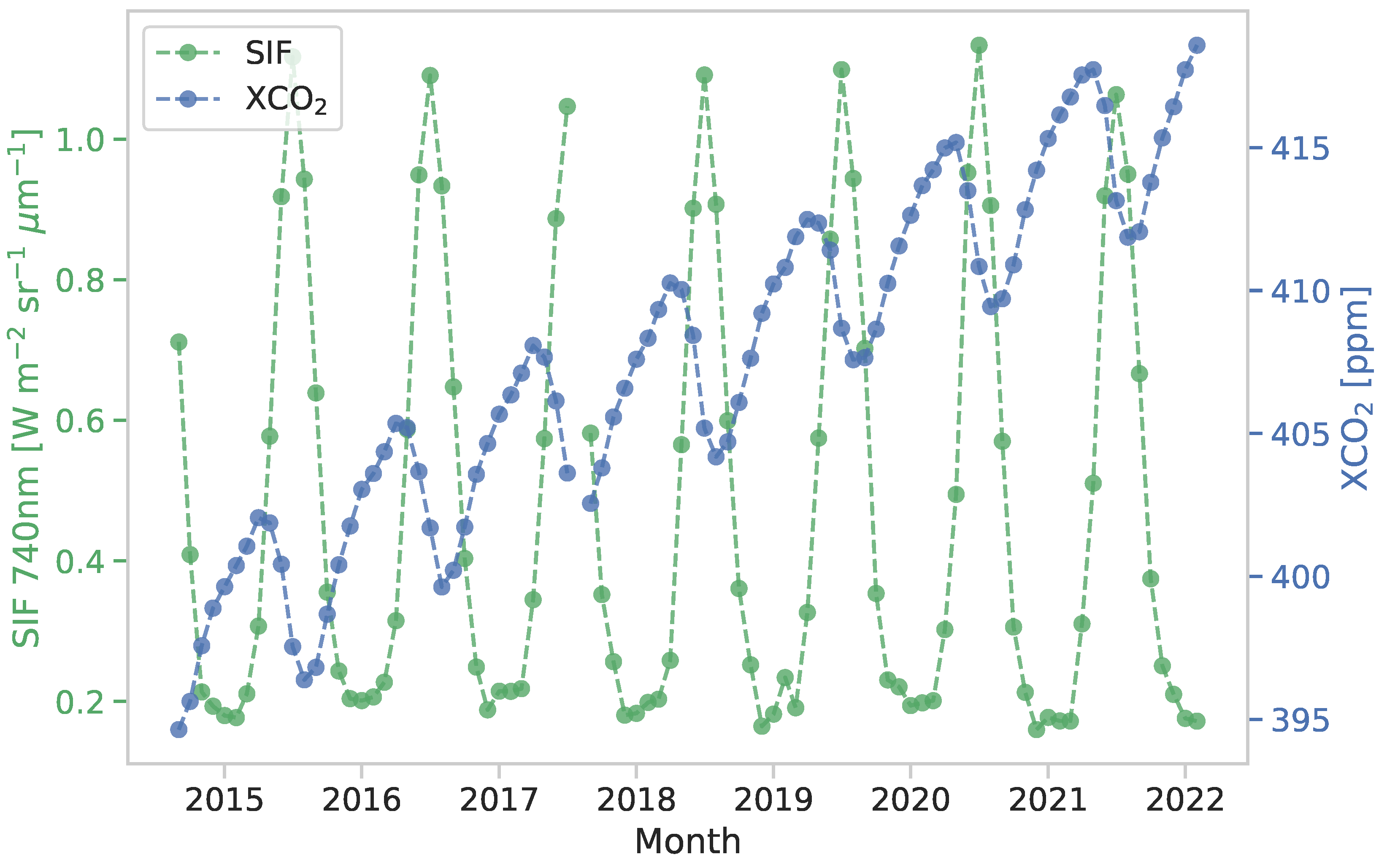
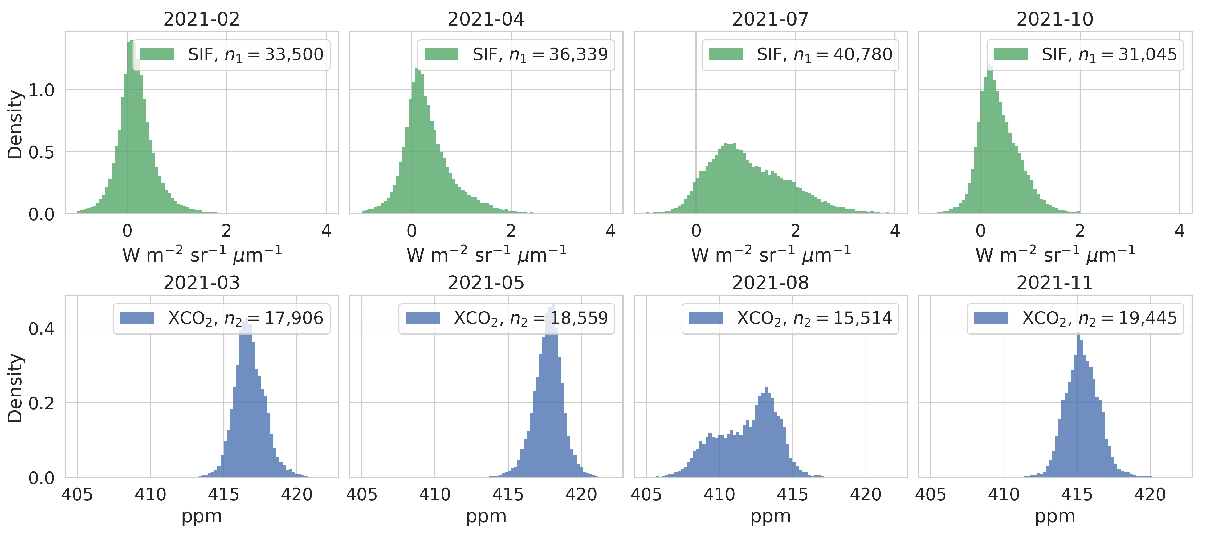
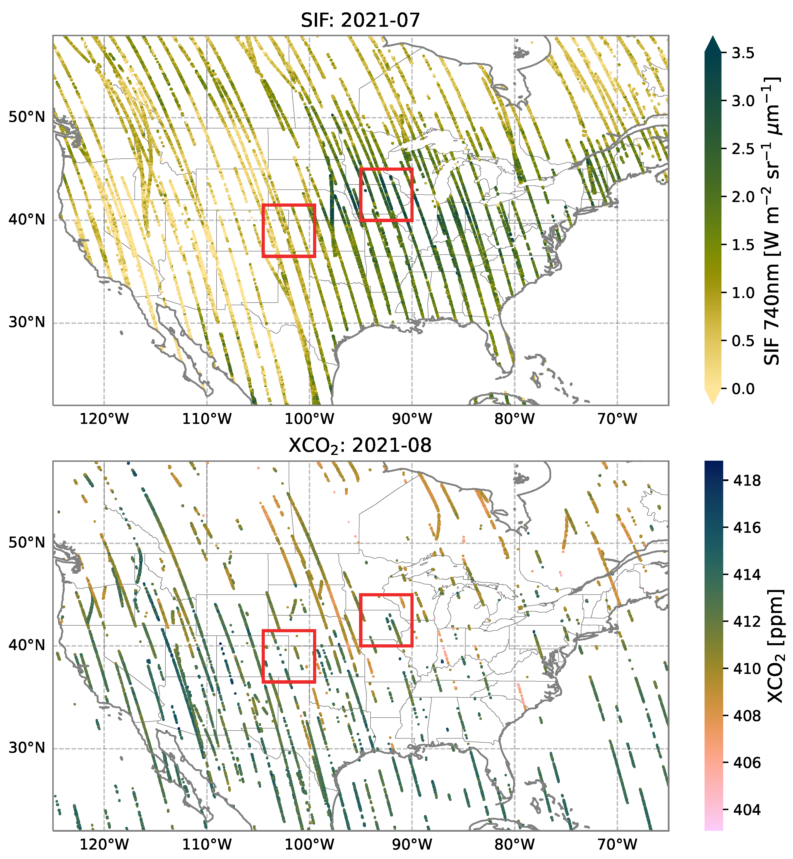
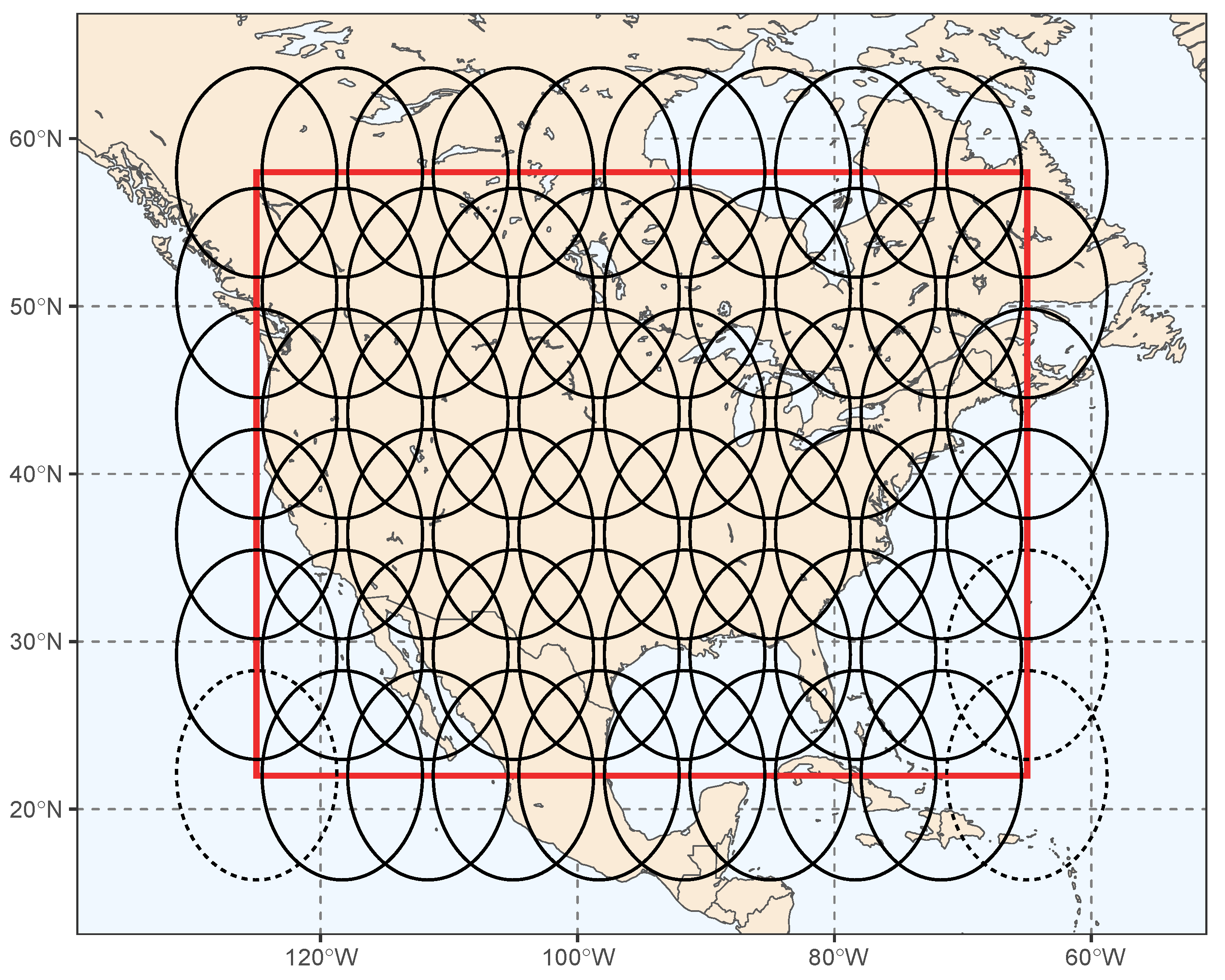
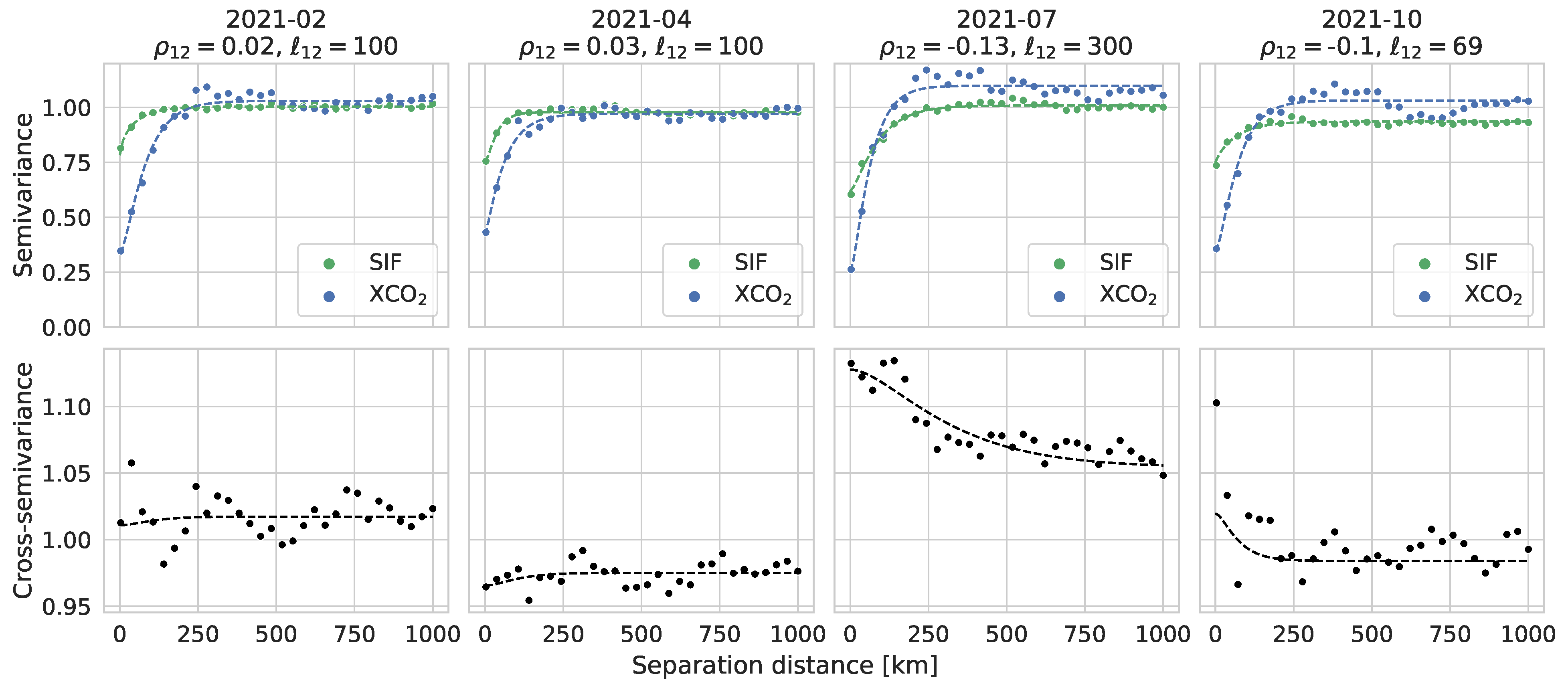
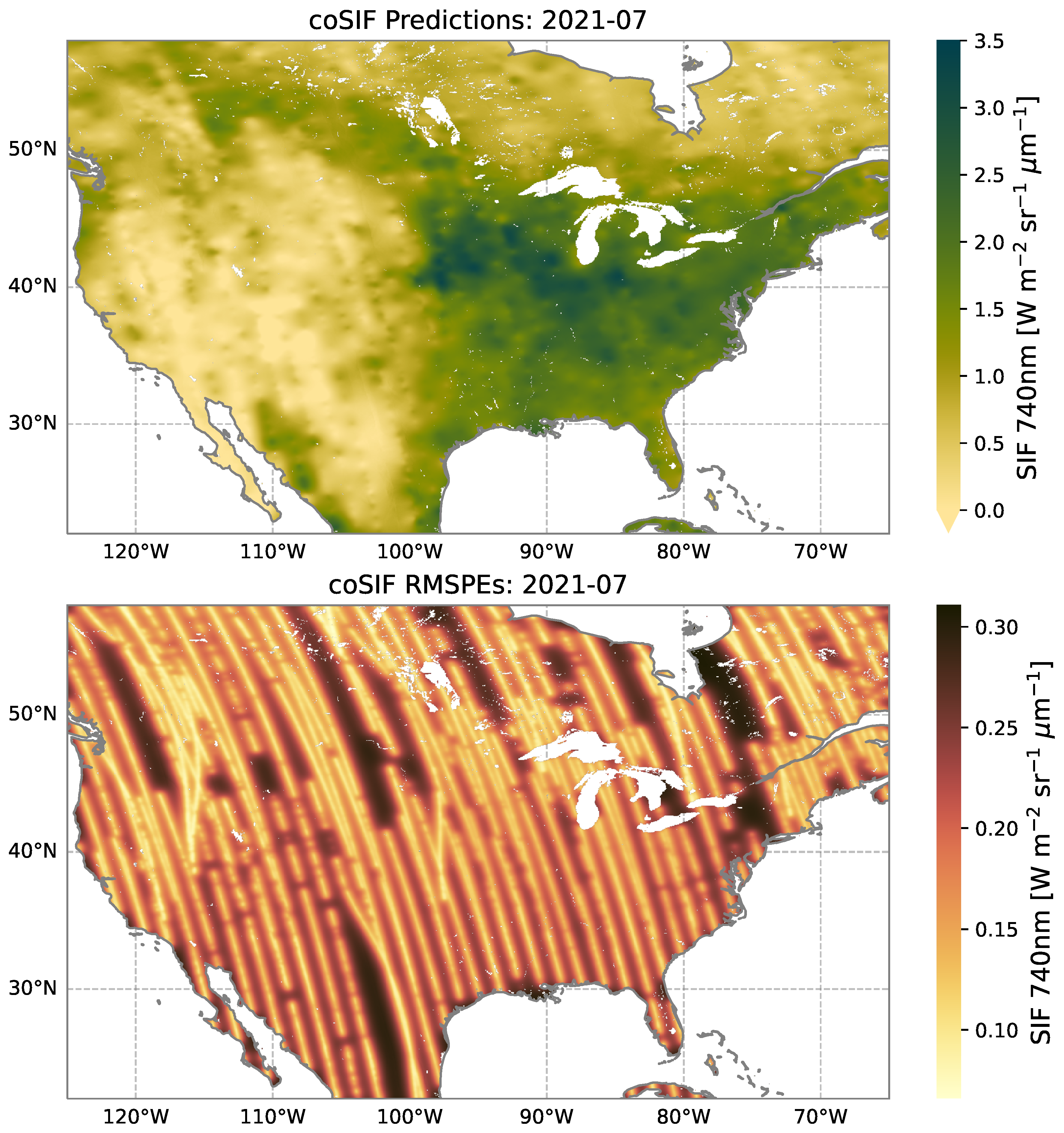
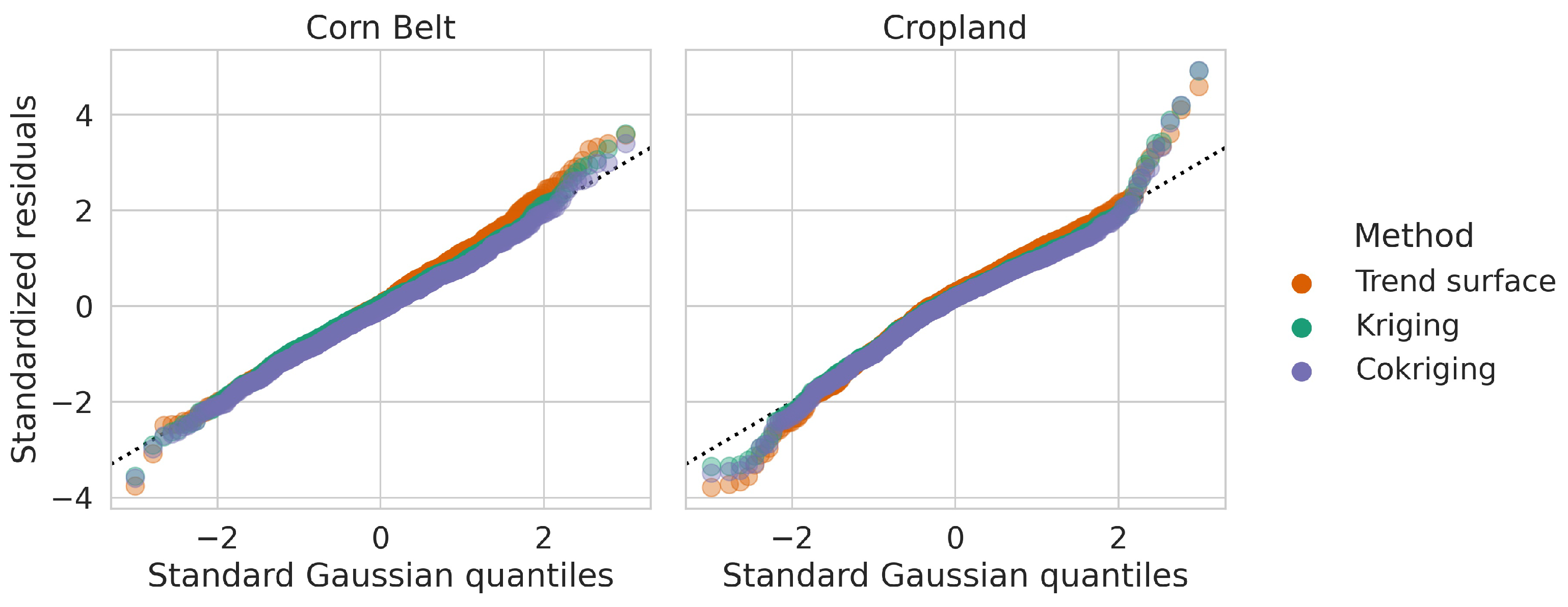
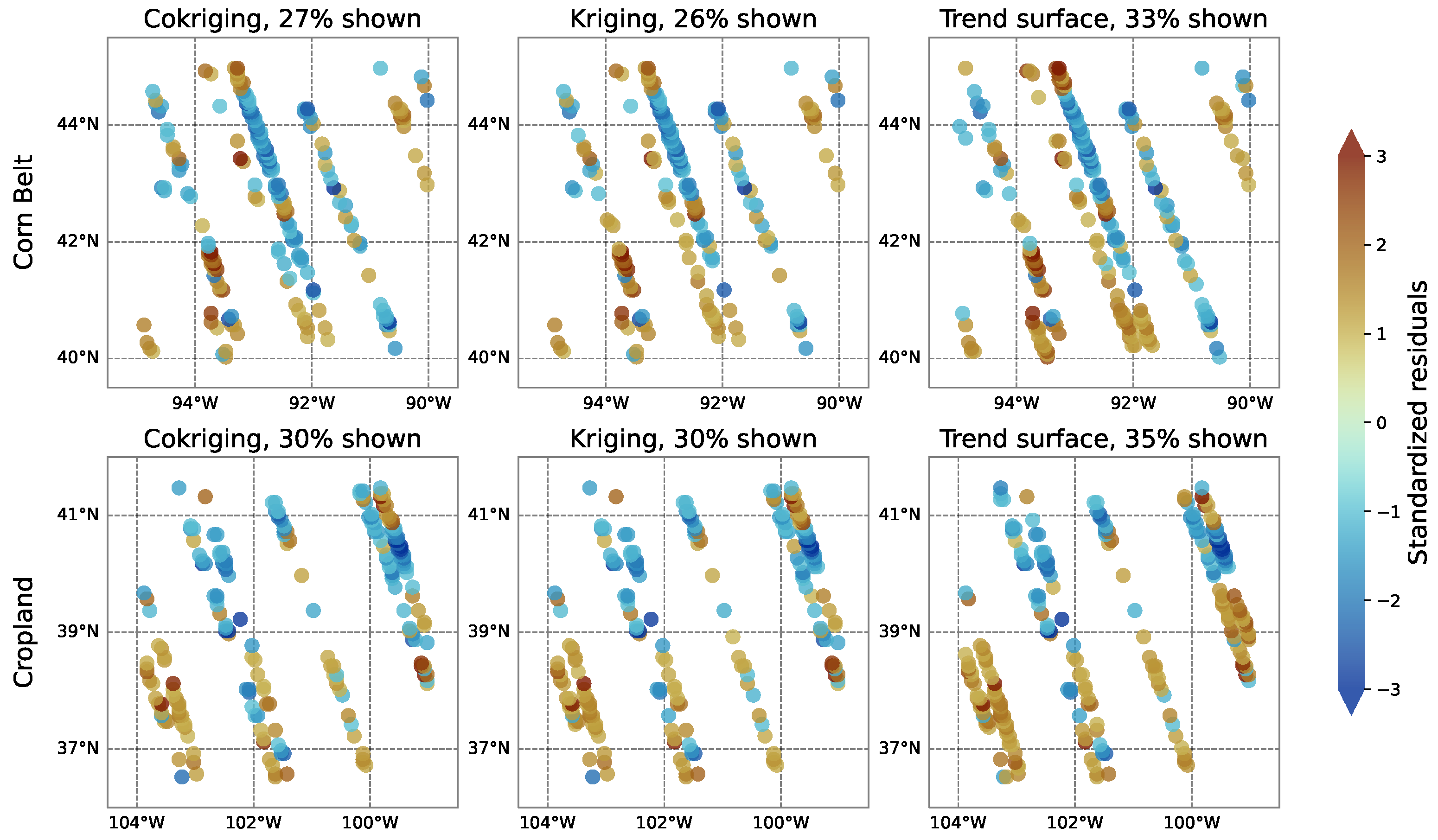
Table 1.
Validation metrics for the Corn Belt and Cropland validation blocks in July 2021. Bold typeface indicates the best performing method according to each metric. Locations of the validation blocks are shown in Figure 3.
Table 1.
Validation metrics for the Corn Belt and Cropland validation blocks in July 2021. Bold typeface indicates the best performing method according to each metric. Locations of the validation blocks are shown in Figure 3.
| Block | Method | BIAS | RASPE | INT | DSS | MDSS |
|---|---|---|---|---|---|---|
| Corn Belt | Cokriging | −0.06 | 0.58 | 2.85 | −0.13 | −311.94 |
| Kriging | −0.01 | 0.59 | 2.93 | −0.12 | −308.63 | |
| Trend surface | 0.03 | 0.62 | 3.03 | 0.03 | 21.32 | |
| Cropland | Cokriging | 0.01 | 0.56 | 2.95 | −0.22 | −356.18 |
| Kriging | 0.03 | 0.56 | 2.93 | −0.20 | −355.44 | |
| Trend surface | 0.07 | 0.60 | 3.05 | −0.08 | −57.77 |
Disclaimer/Publisher’s Note: The statements, opinions and data contained in all publications are solely those of the individual author(s) and contributor(s) and not of MDPI and/or the editor(s). MDPI and/or the editor(s) disclaim responsibility for any injury to people or property resulting from any ideas, methods, instructions or products referred to in the content. |
© 2023 by the authors. Licensee MDPI, Basel, Switzerland. This article is an open access article distributed under the terms and conditions of the Creative Commons Attribution (CC BY) license (https://creativecommons.org/licenses/by/4.0/).
Share and Cite
MDPI and ACS Style
Jacobson, J.; Cressie, N.; Zammit-Mangion, A. Spatial Statistical Prediction of Solar-Induced Chlorophyll Fluorescence (SIF) from Multivariate OCO-2 Data. Remote Sens. 2023, 15, 4038. https://0-doi-org.brum.beds.ac.uk/10.3390/rs15164038
AMA Style
Jacobson J, Cressie N, Zammit-Mangion A. Spatial Statistical Prediction of Solar-Induced Chlorophyll Fluorescence (SIF) from Multivariate OCO-2 Data. Remote Sensing. 2023; 15(16):4038. https://0-doi-org.brum.beds.ac.uk/10.3390/rs15164038
Chicago/Turabian StyleJacobson, Josh, Noel Cressie, and Andrew Zammit-Mangion. 2023. "Spatial Statistical Prediction of Solar-Induced Chlorophyll Fluorescence (SIF) from Multivariate OCO-2 Data" Remote Sensing 15, no. 16: 4038. https://0-doi-org.brum.beds.ac.uk/10.3390/rs15164038
Note that from the first issue of 2016, this journal uses article numbers instead of page numbers. See further details here.