Article

Classification of Coniferous and Broad-Leaf Forests in China Based on High-Resolution Imagery and Local Samples in Google Earth Engine

1
Department of Remote Sensing Science and Technology, School of Electronic Engineering, Xidian University, Xi’an 710071, China
2
Xi’an Key Laboratory of Advanced Remote Sensing, Xi’an 710071, China
3
Key Laboratory of Collaborative Intelligence Systems, Ministry of Education, Xidian University, Xi’an 710071, China
4
Key Laboratory of State Forestry Administration on Soil and Water Conservation & Ecological Restoration of Loess Plateau, Shaanxi Academy of Forestry, Xi’an 710082, China
*
Author to whom correspondence should be addressed.
Remote Sens. 2023, 15(20), 5026; https://0-doi-org.brum.beds.ac.uk/10.3390/rs15205026
Submission received: 21 September 2023 / Revised: 12 October 2023 / Accepted: 15 October 2023 / Published: 19 October 2023
(This article belongs to the Collection Feature Paper Special Issue on Forest Remote Sensing)

Abstract

:
As one of the world’s major forestry countries, accurate forest-type maps in China are of great importance for the monitoring and management of forestry resources. Classifying and mapping forest types on a large scale across the country is challenging due to the complex composition of forest types, the similarity of spectral features among forest types, and the need to collect and process large amounts of data. In this study, we generated a medium-resolution (30 m) forest classification map of China using multi-source remote sensing images and local samples. A mapping framework based on Google Earth Engine (GEE) was constructed mainly using the spectral, textural, and structural features of Sentinel-1 and Sentinel-2 remote sensing images, while local acquisition data were utilized as the mapping channel for training. The proposed method includes the following steps. First, local data processing is performed to obtain training and validation samples. Second, Sentinel-1 and Sentinel-2 data are processed to improve the classification accuracy by using the enhanced vegetation index (EVI) and the red-edge position index (REPI) computed based on the S2A data. Third, to improve classification efficiency, useless bands are removed and important bands are retained through feature importance analysis. Finally, random forest (RF) is used as a classifier to train the above features, and the classification results are used for mapping and accuracy evaluation. The validation of the samples showed an accuracy of 82.37% and a Kappa value of 0.72. The results showed that the total forest area in China is 21,662,261.17 km 2 , of which 1,127,294.42 km 2 of coniferous forests account for 52% of the total area, 981,690.98 km 2 of broad-leaf forests account for 45.3 % of the total area, and 57,275.77 km 2 of mixed coniferous and broad-leaf forests account for 2.6% of the total area. Upon further evaluation, we found that textural and structural features play a greater role in classification compared to spectral features. Our study shows that combining multi-source high-resolution remote sensing imagery with locally collected samples can produce forest maps for large areas. Our maps can accurately reflect the distribution of forests in China, which is conducive to forest conservation and development.

1. Introduction

Forests cover almost one-third of the world’s land area and constitute the main body of the terrestrial ecosystem with the largest coverage, the widest distribution, the most complex composition, the richest biodiversity, and the highest primary productivity [1,2]. As one of the world’s largest developing countries, China’s rich and diverse forest resources are of great significance to the country’s sustainable development and the protection of the ecological environment. Forest classification plays an important role in the management and conservation of forest resources and carbon storage [3]. Coniferous forests are usually considered the early stage of forest succession, broad-leaf forests the late stage of forest succession, and mixed coniferous and broad-leaf forests the transitional stage of forest succession [4,5]. Coniferous and broad-leaf forests have different characteristics above and below ground. Coniferous forests are characterized by tree species with needle-like foliage, a leaf pattern that helps reduce water evaporation in cold climates. Broad-leaf forest species, on the other hand, usually have broad, spreading leaves; are more sensitive to light; and are usually found in warmer regions [6]. However, most existing forest studies do not distinguish between coniferous forests, broad-leaf forests, and mixed coniferous and broad-leaf forests on a large scale. Therefore, in order to better understand the specific distribution of forests in China, a nationwide mapping of coniferous, broad-leaf, and mixed coniferous and broad-leaf forests in China is needed.
China has a vast land area and a diverse geomorphologic environment that provides a wide variety of habitats for different vegetation types [7,8]. As a result, there is a great deal of variation in the composition and distribution range of China’s forests, and these factors make it extremely difficult to obtain ground vegetation information [9,10]. Traditional methods of obtaining vegetation information such as ground surveys and sampling are inefficient, laborious, and costly, and they fail to provide a continuous spatial data distribution of ground vegetation [11]. Moreover, the scale of the survey samples is inconsistent with the scale of the actual forest, making it difficult to meet accuracy requirements. Therefore, technologies such as big data, machine learning, and remote sensing are increasingly applied in intelligent forestry [12,13].
Remote sensing data have provided increasing amounts of multispectral data since the launch of the Sentinel mission [14]. Earth observation satellites not only monitor and periodically revisit the ground but can also provide complete spatial details for forest mapping. In early studies, supervised maximum likelihood classifiers (MLC) and unsupervised clustering (K-means) were generally used [15,16]. After 1995, classifiers based on nonparametric decision trees and neural networks, among others, gradually replaced traditional methods and were able to better cope with the complexity of remotely sensed data [17,18]. In recent years, remote sensing research has increasingly favored the use of nonparametric machine learning methods such as random forest (RF) and support vector machine (SVM) [19]. These methods are able to handle mixed sets of input variables (spectral, texture, ensemble, exponential, etc.), and the improvement of hardware and software capabilities has facilitated the application of these methods [20]. Therefore, machine learning classification methods are currently regarded as effective for remote sensing image classification and processing. Many studies have utilized sets of input variables, i.e., features, to map forests. For example, Descals et al. combined spectral and textural features to map closed-canopy oil palm plantations globally [21]. Zhao et al. combined optimal phenological period, spectral, and topographic features to map grassland classifications in Zambia. Despite the rapid development of the hyperspectral remote sensing of vegetation, it has not been widely explored for large-scale forest remote sensing classification [22].
The aim of this study is to produce a national forest classification map with a resolution of 30m. The work was realized on the Google Earth Engine platform, which is a computing cloud platform provided free of charge by Google since 2010 that archives a large amount of satellite imagery and provides geographic cloud computing for geoscience applications on a global scale [23]. Since the remote sensing datasets on the GEE platform are very large, the selection of datasets is also important. Remote sensors have their own characteristics, and using different remote sensing images may lead to different results, even if the study objectives are the same. We chose Sentinel data as the remote sensing data for this study. The Sentinel-1 satellites are a crucial component of Earth observations that are equipped with C-band synthetic aperture radar (SAR) technology, which offers a unique capability to provide continuous imagery regardless of lighting conditions or weather patterns, making them exceptionally valuable for a wide range of applications. The satellites provide imagery with a revisit period of 12 days during frequent monitoring of the Earth’s surface [24,25]. Each scene captures imagery at multiple resolutions, offering users flexibility in selecting the level of detail required for their specific applications. The available resolutions include 10 m, 25 m, and 40 m, enabling fine- to medium-scale monitoring and analysis. The scenes are also characterized by different polarization options, which enable the collection of data on how radar waves interact with the Earth’s surface. Both single-polarization (HH or VV) and dual-polarization (HH+HV or VV+VH) operations are supported, and they are implemented via a transmitter chain (switchable to H or V) and two parallel receiver chains for H and V polarizations. Sentinel-2 was launched on 23 June 2015 as the second satellite of the Global Monitoring for Environment and Security (GMES) program. The satellite carries a multispectral imager covering 13 spectral bands with a width of 290 km and monitors the Earth at three resolutions (10, 20, and 60 m). One satellite has a revisit period of 10 days, and two satellites have a revisit period of 5 days, opening up a completely new way of specialized forest monitoring [26]. The relatively short revisit period enables the collection of more detailed information on individual forest types. Due to a variety of satellites and sensors, S2 data have led to innovations in the field of remote sensing and have seen a wide range of applications.
The noteworthy contributions of this study are as follows: (1) Optimal feature combination—Based on all bands of the original Sentinel-2 image, the EVI and REPI indices are calculated, and texture feature extraction is completed. (2) Feature importance analysis—In order to ensure the computational efficiency of the network, we verify the accuracy according to the order of importance of the band features, retaining the high-quality feature bands and removing the redundant bands. (3) Combination of multi-source high-resolution remote sensing data and local samples to construct a framework for the large-scale drawing of classification maps on the GEE platform. (4) Generation of a classification map of coniferous forests, broad-leaf forests, and mixed coniferous and broad-leaf forests in China in 2020 with a resolution of 30m. The resulting classification map has significant implications for forest protection, conservation, and development efforts in China. It provides a comprehensive overview of forest types and their distribution, serving as a crucial resource for policymakers, researchers, and conservationists. Additionally, the map facilitates informed decision making in sustainable forest management, ecosystem conservation, and land-use planning. In summary, this study’s outcomes contribute to the better understanding and responsible management of China’s diverse and vital forest resources.

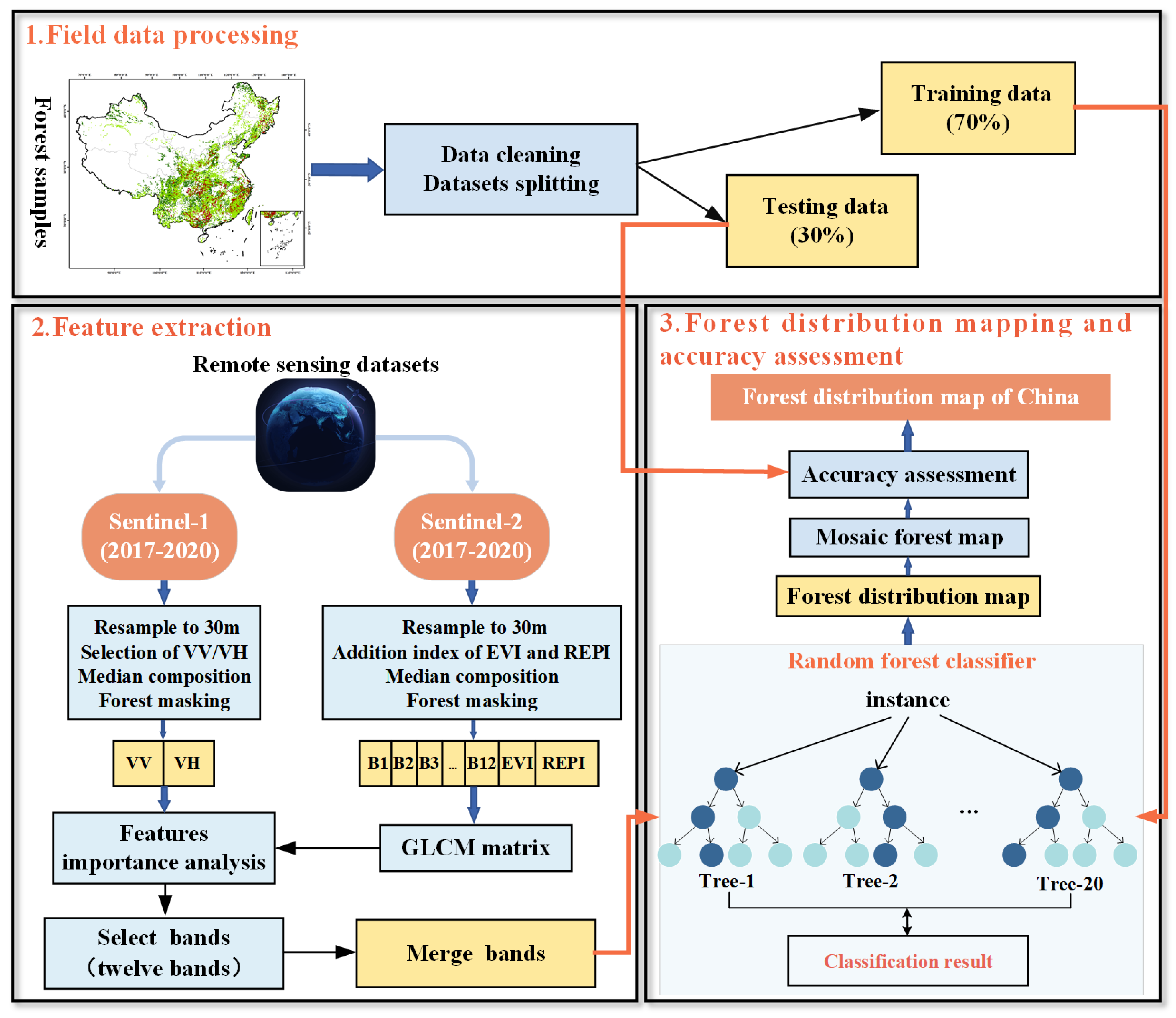
2. Materials and Methods
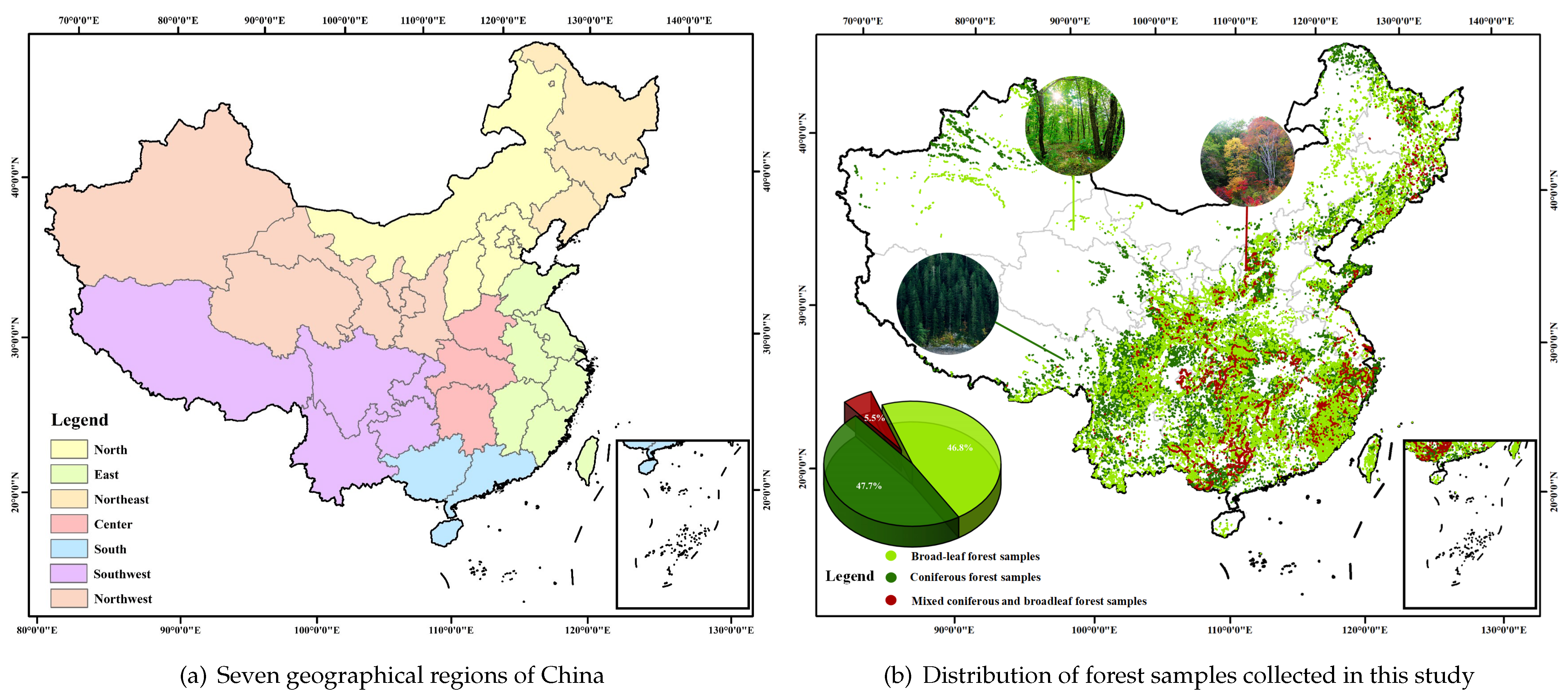
The forest classification process (Figure 1) encompasses the following three distinct steps, each playing a critical role in achieving accurate and reliable results: Step 1—preprocessing and categorization of forest collection samples. Step 2—feature extraction using remote sensing datasets. Step 3—mapping and accuracy assessment of Chinese forest classifications. The detailed process of each step is described below.

2.1. Field Data

We used a mobile phone application (LiVegetation) and forest data collected from the literature [27]. This application enabled the systematic recording of vegetation attributes, along with their corresponding geographical coordinates. Importantly, all the data collected through LiVegetation were meticulously gathered by scholars or experts in vegetation ecology. This ensured the quality and accuracy of the recorded information. To enrich our dataset, we reviewed scientific papers related to nature reserves and recent biodiversity research books published within the last five years. Our selection retained records that contained specific species composition information and geographic location data. These records were then digitized for further analysis. In total, we collected a substantial dataset comprising 311,890 data. To ensure the dataset’s suitability for forest classification, we screened and categorized the data (Figure 2b). This categorization process resulted in the following distribution: 145,938 coniferous forest samples, 145,938 broad-leaf forest samples, and 17,227 mixed coniferous and broad-leaf forest samples. Each of these samples was associated with precise geographic coordinates, allowing for precise spatial analysis. These data were reprojected, resulting in the division of China into seven regions (Figure 2a). Detailed information about each region is shown in Table 1. The label of the coniferous forest area is “0”, the label of the broad-leaf forest area is “1”, and the label of the mixed coniferous and broad-leaf forest area is “2”. Then, we divided the forest samples into training data (70%) and validation data (30%).

2.2. Remote Sensing Datasets

2.2.1. Sentinel-1

The Sentinel-1 Ground Range-Detected (GRD) data used in our study were accessed through the Google Earth Engine (GEE) system. This is a ground range monitoring product that captures amplitude information and has a multiview capability to minimize the effects of speckle. Due to their sensitivity to the vegetation structure, the VV and VH polarization bands of the Sentinel-1 time-series images from 2017 to 2020 were selected to generate a complete VV and VH image of the whole of China for classification using the median synthesis method. This image was resampled to 30 m for spatial analysis, followed by feature importance analysis.

2.2.2. Sentinel-2

In the context of our research, we used Sentinel-2 Multispectral Instrument (MSI) Level 2A data, which were accessed through the Google Earth Engine (GEE) platform. This particular dataset has been meticulously calibrated using a digital elevation model. Each pixel’s value is derived from measurements acquired at the Top of Atmosphere (TOA), with data records extending back to 2017. However, it is noteworthy that some geographical regions experience partial gaps in remote sensing data due to cloud cover. Figure 3 shows the remote sensing image coverage of Sentinel-2 in China from 8 March 2017 to 31 December 2020. A detailed description of the Sentinel 2 band is detailed in Appendix A.1.
The dataset encompasses an array of spectral bands, including visible and near-infrared (NIR) bands (B2, B3, B4, B8) with a spatial resolution of 10 m per pixel. Additionally, it incorporates short-wave infrared bands (B11, B12) with a resolution of 20 m per pixel. Notably, band 1 serves the purpose of aerosol analysis, whereas bands 9 and 10 are optimally suited for identifying water vapor and cirrus clouds. These specific bands provide imagery at a resolution of 60 m per pixel, predominantly intended for atmospheric correction procedures. Augmenting the dataset further are three quality assessment (QA) bands, with QA60 being particularly significant due to its inclusion of cloud mask information. This information proves invaluable in the removal of cirrus and dense cloud formations from the images.

2.2.3. Auxiliary Data

In our research, we employed forest masks derived from GlobeLand30’s 2020 land cover product [28]. These forest masks are important in our analysis as they help delineate areas of coniferous, broad-leaf, and mixed coniferous and broad-leaf forests within forested regions. This approach serves to minimize the influence of other land cover types and significantly enhances the accuracy of our forest classification processes.

2.3. Methodology

2.3.1. Structural and Spectral Feature Analysis

In this article, the VV and VH polarization bands of the S1 time-series images from 2017 to 2020 were selected due to their sensitivity to the vegetation structure [29]. The median synthesis method was used to generate a complete VV and VH image covering the whole of China, which was then resampled to a resolution of 30 m.
S2 data with less than 10% cloud cover from 2017 to 2020 were selected to extract spectral and image texture features of the study area for mapping the forest distribution in China. Before further processing, cloud masking and shading were applied to each image for quality assessment using the default values provided by GEE. Then, a synthetic image was obtained by calculating the median value of each pixel. The synthetic image was resampled to a resolution of 30 m. Two vegetation indices that help distinguish coniferous forests, broad-leaf forests, and mixed coniferous and broad-leaf forests were added, including the enhanced vegetation index (EVI) and the red-edge position index (REPI), which were computed using the following equations:
E V I = 2.5 × ρ N I R ρ R e d ρ N I R + 6 × ρ R e d ρ B l u e + 1
R E P I = 705 + 35 × ( ρ R e d ρ R e d E d g e 3 ) / 2 ρ R e d E d g e 2 ρ R e d E d g e 2 ρ R e d E d g e 1
The EVI index is more sensitive to canopy structure and type changes [30]. It also reduces the influence of atmospheric and soil noise and provides a stable response to the vegetation in the area measured. Due to scattering from the leaves and canopy, the reflectance of vegetation in the red-edge range (680–780 nm) increases sharply with the wavelength [31], and the reflectance near the red edge is sensitive to crops’ chlorophyll and nitrogen content. The REPI corresponds to the wavelength position, where the reflectance of the green vegetation in the red-edge range has the fastest increase in reflectance with the increasing wavelength. Compared with the NDVI, where saturation is a problem, the REPI corresponds more significantly to the leaf area index and chlorophyll concentration [32].

2.3.2. Texture Features Analysis

The classification of forests based solely on spectral features is inefficient due to the potential for different objects to exhibit similar spectral characteristics. Additionally, the same object may display varying spectral attributes under different conditions, such as diverse angles of sunlight, densities, and water contents [33].
Texture is a crucial attribute of an image, representing patterns resulting from spatial variations in grayscale levels. One widely employed method for texture characterization is the gray-level covariance matrix (GLCM). The GLCM defines the joint probability distribution of gray levels for two pixels with specific spatial relationships within an image [34]. Google Earth Engine (GEE) offers a rapid computational function called “glcmTexture”, which employs GLCM texture features. It calculates texture metrics based on the covariance matrix of grayscale values around each pixel in every band.
The GLCM is essentially a table that depicts the frequency of diverse combinations of pixel luminance values (gray levels) within an image. It tallies the occurrences of a pixel, with value X being adjacent to a pixel with value Y at a particular direction and distance, and then extracts statistics from this dataset. The implementation computes 14 GLCM metrics initially proposed by Haralick [35], along with an additional 4 metrics introduced by Conners [36]. The resulting output comprises 18 bands for each input band if direction averaging is enabled, and 18 bands for every direction pair within the kernel if this feature is not enabled. These metrics include the Angular Second Moment (ASM), Contrast (CONTRAST), Correlation (CORR), Variance (VAR), Inverse Difference Moment (IDM), Sum Average (SAVG), Sum Variance (SVAR), Sum Entropy (SENT), Entropy (ENT), Difference Variance (DVAR), Difference Entropy (DENT), Information Measure of Correlation (IMCORR1 and IMCORR2), Max. Correlation Coefficients (MAXCORR), Dissimilarity (DISS), Inertia (INERTIA), Cluster Shading (SHADE), and Cluster Prominence (PROM) [37]. Here are some formulas for calculating these metrics:
A S M = i j p 2 ( i , j )
C o n t r a s t = n = 0 N g 1 n 2 [ i = 1 N g j = 0 N g p ( i , j ) ]
C o r r e l a t i o n = i j ( i , j ) p ( i , j ) μ x μ y σ x σ y
V a r i a n c e = i j ( i u ) 2 p ( i , j )
I D M = i j ( 1 1 + ( i j ) 2 ) p ( i , j )
S A V G = i = 2 2 N g ( i p ( x + y ) ( i ) )
E n t r o p y = i j p ( i , j ) l o g ( p ( i , j ) )
D I S S = n = 1 N g 1 n [ i = 1 N g j = 1 N g p ( i , j ) 2 ]
where p(i,j) is the (I,j)th entry in a normalized gray-tone spatial-dependence matrix; N g is the number of distinct gray levels in the quantized image; μ x and μ y are the means of p x and p y ; and σ x and σ y are the standard deviations of p x and p y .
Following the aforementioned feature extraction process, texture feature extraction was performed on the S2 image. This resulted in the generation of 18 texture indices for each band, culminating in a total of 252 bands.

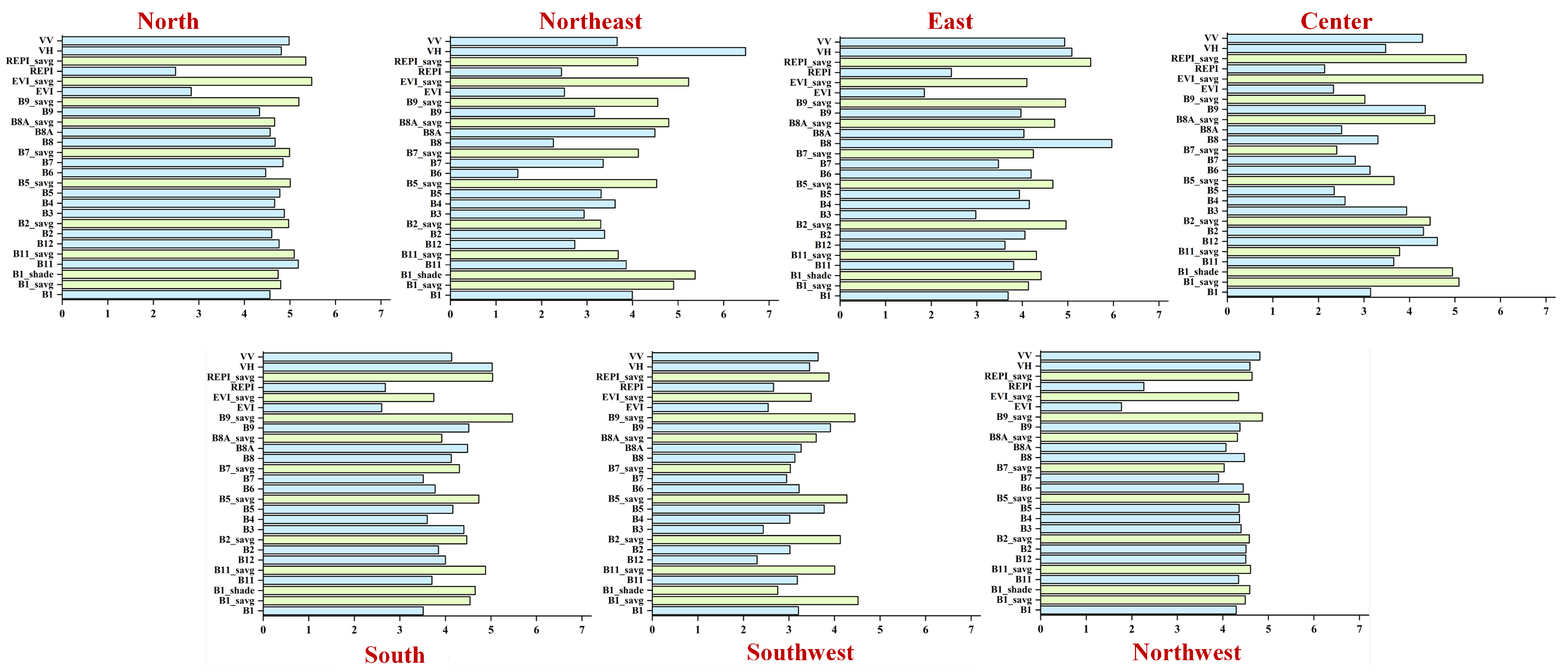
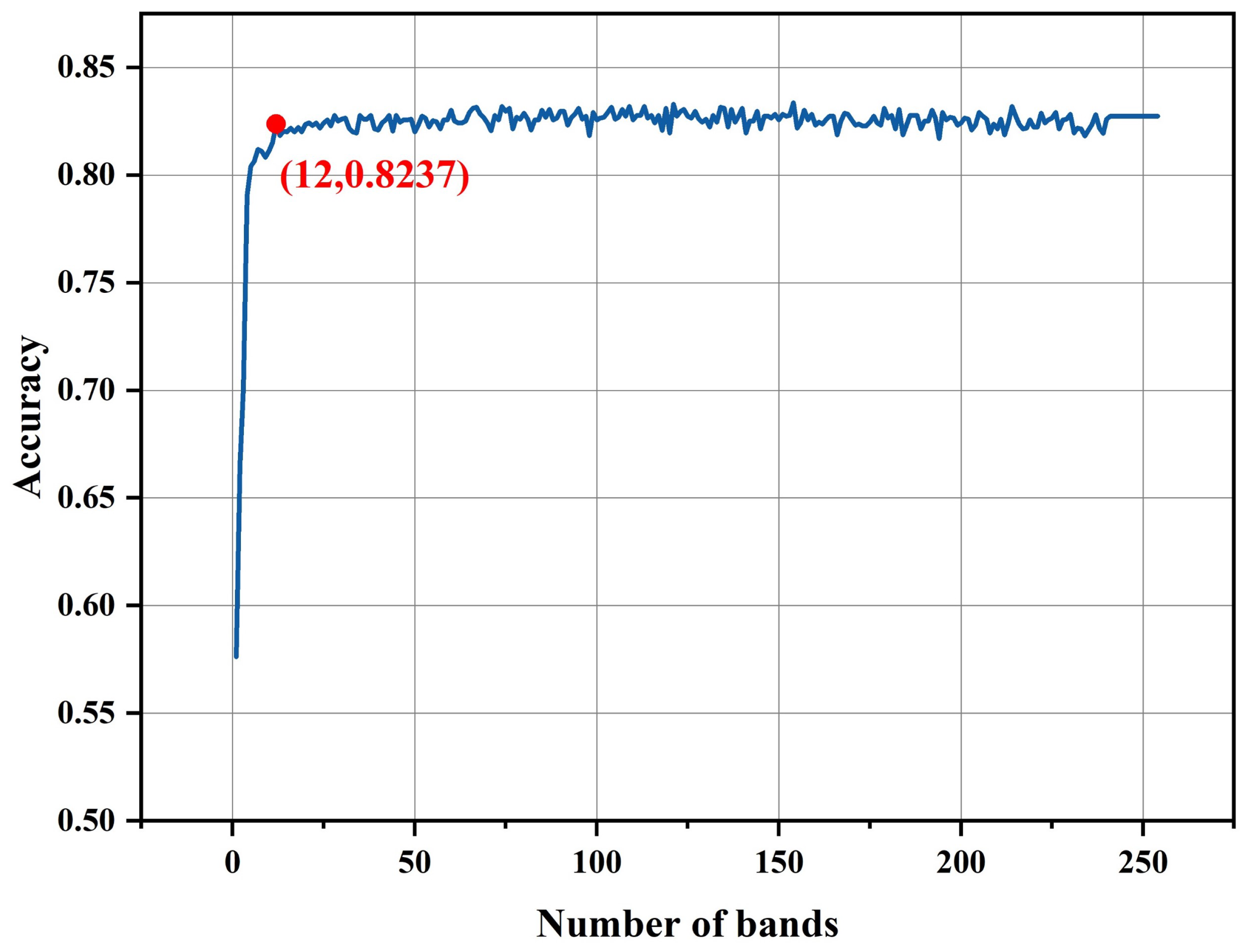
2.3.3. Feature Importance Analysis

Despite obtaining an extensive array of both spectral and texture features, an excess of texture attributes can lead to redundancy and computational inefficiency. Hence, a feature selection process is imperative to retain crucial attributes while discarding irrelevant ones. To ascertain the quality of features, the “explain” function, integrated within the GEE platform, was employed to evaluate the significance of 254 features. Table 2 shows the results of the analysis for the first 18 bands in the study area, where higher values correspond to increased feature importance. The results show that none of the 14 MAXCORR bands played any role in the classification, which is evident from their importance score of 0. Conversely, the SAVG demonstrates substantial importance across all bands, significantly outweighing other attributes. Let us delve into the significance of a feature by examining its variable importance measure based on out-of-bag data ( V I M j O O B ) [38]. V I M j O O B is a metric defined as follows: During the random forest (RF) modeling process, out-of-bag (OOB) data are utilized. This involves randomly selecting training bootstrap samples to construct a decision tree within each tree of the random forest. Once a tree is built, the OOB prediction error rate is computed. Subsequently, the observations of the variable Xj are randomly permuted and the tree is recalculated, along with the OOB prediction error rate. Finally, the difference between the two OOB error rates is computed. This process is repeated across all trees within the random forest ensemble, and the resulting differences are standardized and averaged to derive the variable importance measure based on out-of-bag data ( V I M j O O B ) for the variable X j . In essence, V I M j O O B provides an assessment of the impact of each individual variable ( X j ) on the model’s predictive performance. It quantifies how perturbing the values of X j affects the accuracy of predictions, taking into account the inherent variability introduced by the random forest modeling process [39].
The variable X j in the i-th tree V I M j O O B is:
V I M j O O B = p = 1 n o i I ( Y p = Y p i ) n o i p = 1 n o i I ( Y p = Y p , π j i ) n o i
where n o i is the number of observations in the out-of-bag (OOB) data of the i-th tree; I(g) is the indicator function, which equals 1 when two values are equal and 0 when they are not; Y p is a binary variable, taking values of 0 or 1, which represents the true outcome of the p-th observation; Y p i is another binary variable, indicating the prediction result of the p-th observation of the OOB data by the i-th tree before any random replacement; and Y p , π i denotes the prediction result of the i-th tree on the p-th observation of the OOB data after random replacement. If the variable j does not appear in the i-th tree, then the variable importance measure based on out-of-bag data ( V I M j O O B ) for that variable is assigned a value of 0.
The results of the importance analysis of the spectral, texture, and structural features for each region are shown in Figure 4. Most of the texture feature values are higher than the spectral feature values, so compared with the spectral features, the texture information helps distinguish between coniferous, broad-leaf, and mixed coniferous and broad-leaf forests. The structural features VV and VH also show good importance, so we choose texture features and structural features to input into the network. It can be seen from the table that structural features performed better in the northeast, east, and south, whereas the spectral features performed better in the center.
For the 254 bands obtained by sorting according to the importance of features, we started with one band and increased by one band step by step until all the bands were input into the network. The results are shown in (Figure 5). The accuracy was 59.90% when only the B1_savg band with the highest eigenvalue score was input. However, as the number of bands input into the network increased, the accuracy also increased. When the bands with the top 12 eigenvalue scores were input, the accuracy reached a small peak at 82.37%. At this time, the network took less time to perform computations, and the computations were more efficient. As the number of bands continued to increase, the accuracy experienced some minor fluctuations and mostly stayed around 82.4%. This shows that the increase in the number of bands caused redundancies in the results and a gradual increase in the network computation time, greatly weakening computational efficiency. In the figure, it can be seen that the accuracy was close to 83%, but we chose the optimal case considering the efficiency of the network and the time problem. Therefore, the first 12 bands (B1_savg, B2_savg, B1_shade, B7_savg, B5_savg, EVI_savg, B9_savg, VV, VH, B8A_savg, REPI_savg, and B11_savg) were selected as the final input features.

2.3.4. Classification

In this study, a random forest (RF) approach was used to classify the forests. The RF classifier uses an ensemble of trees, which surpasses the maximum likelihood and decision tree approaches in terms of accuracy. Moreover, the random selection of features and samples is performed within the RF classifier, which effectively avoids the problems of overfitting and excessive dimensionality [40]. We created the RF classifier on the GEE platform with 100 decision trees and a bag fraction of 0.2.

2.4. Accuracy Assessment

2.4.1. Comparison with Field Data

In this article, 30% of the forest samples were used as the validation set, which contained 44,617 coniferous forest samples, 43,781 broad-leaf forest samples, and 5168 mixed coniferous and broad-leaf forest samples. The accuracy of the maps was assessed by calculating the confusion matrix, which is a cross-tabulation of the semi-automatic mapping process and the assignment of class labels to the reference data. In order to check the reliability of the mapping method, we used three metrics: the overall accuracy (OA), Cohen’s consistency index (Kappa coefficient) [41], and macro-F1 score. The OA is the proportion of all reference pixels that are correctly categorized, reflecting the accuracy of the categorization. The Kappa coefficient, as a consistency test, can be used to measure the effectiveness of the categorization. The macro-F1 score is the average F1 value across all categories, which assigns the same weight to all categories, ignoring the actual frequency of occurrence of the sample. The formulas are as follows:
O A = N u m c o r r e c t S u m
K a p p a = P o P e 1 P e
F 1 s c o r e i = 1 1 2 ( 1 P A i + 1 U A i ) = 2 P A i × U A i P A i + U A i
m a c r o F 1 = F 1 s c o r e 1 + F 2 s c o r e 2 + F 3 s c o r e 3 3
where N u m c o r r e c t is the number of correctly mapped validation samples, and Sum is the total number of validation samples. P o is the prediction accuracy, i.e., the ratio of the number of correct samples in each category to the total number of samples; and P e is the chance consistency. PA is the producer’s accuracy, and UA is the user’s accuracy.

2.4.2. Comparison with National Vegetation Map

To further validate the obtained classification map, we compared it with China’s publicly available vegetation map (1:1 million) (2019) [42]. This map presents a complete picture of China’s vegetation, including 55 vegetation types, 960 community types, and the distribution of more than 2,000 dominant plants. Our classification map was resampled to 1,000,000m to match the resolution of the vegetation map. Then, pixel-by-pixel comparisons of the two maps were performed, and the overlapping area was analyzed to verify the spatial extent of our classification map.

3. Results

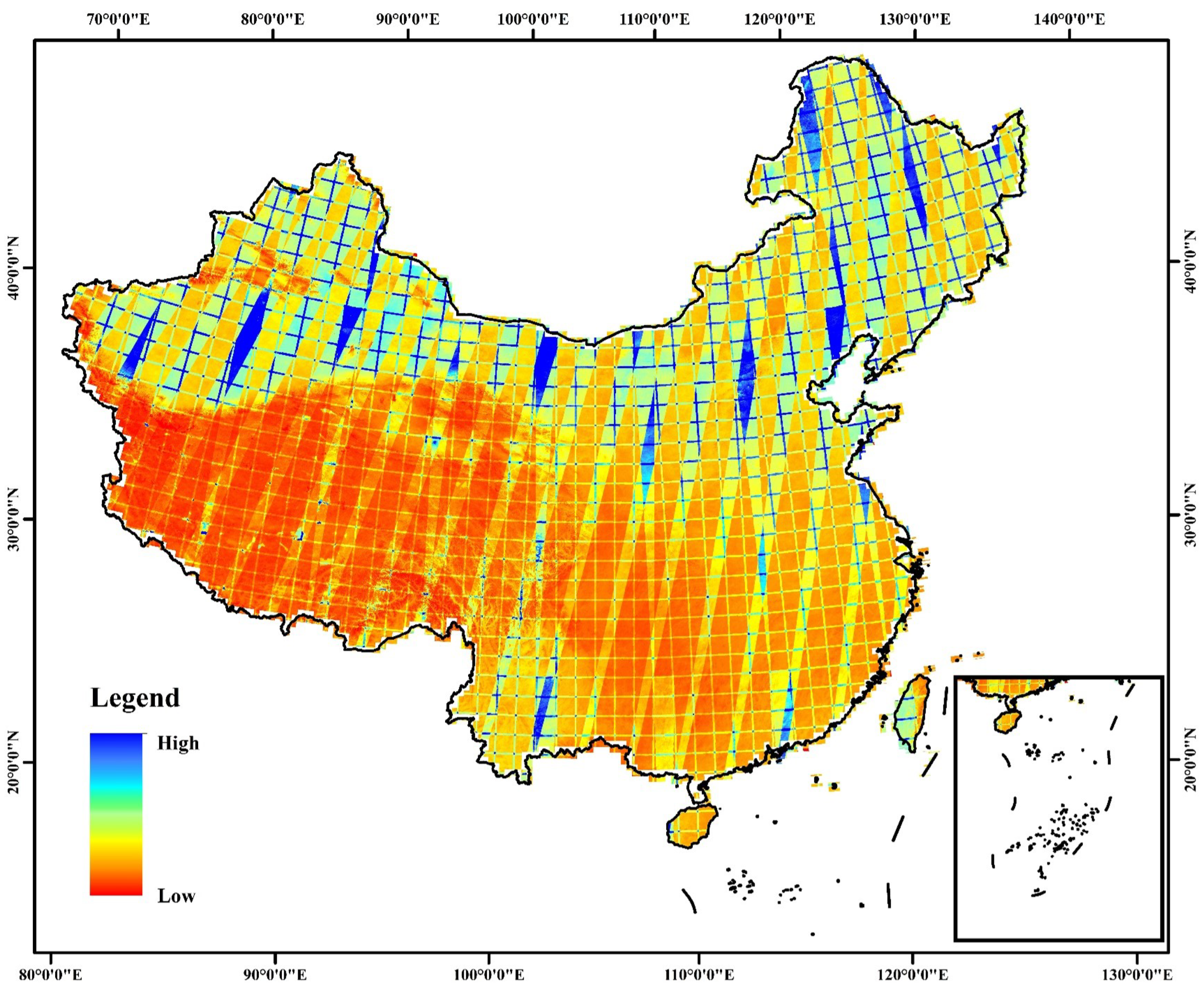
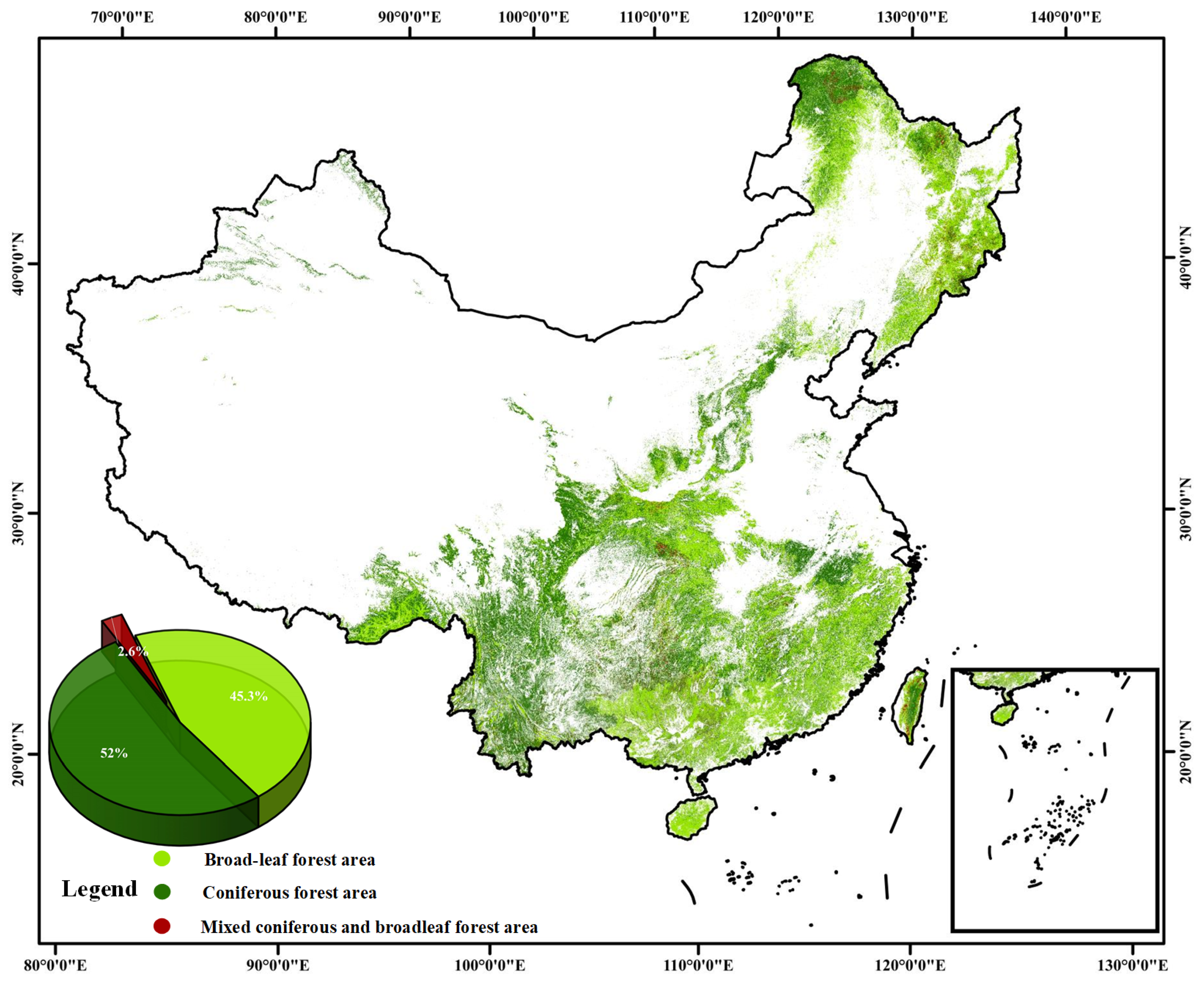
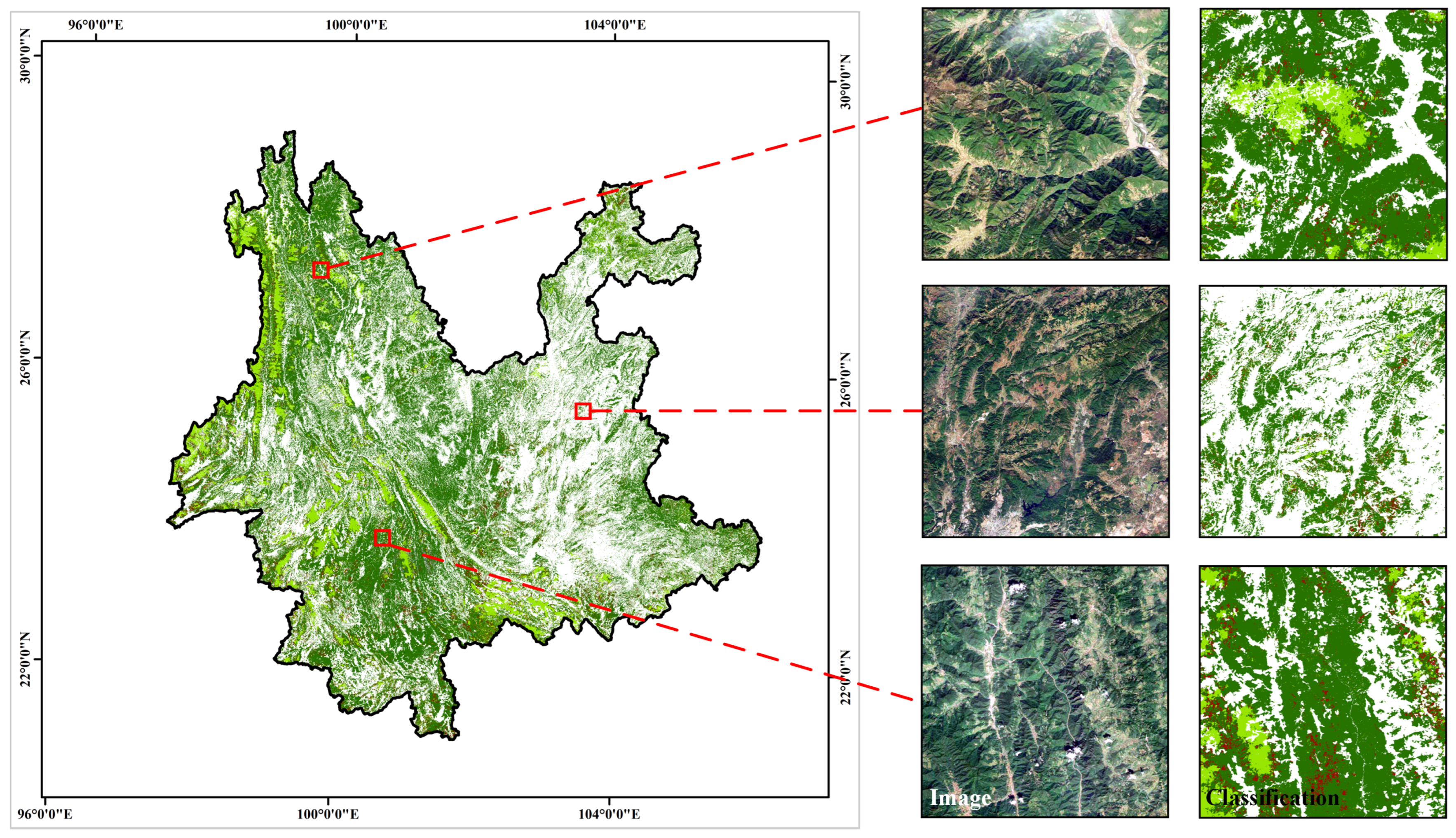
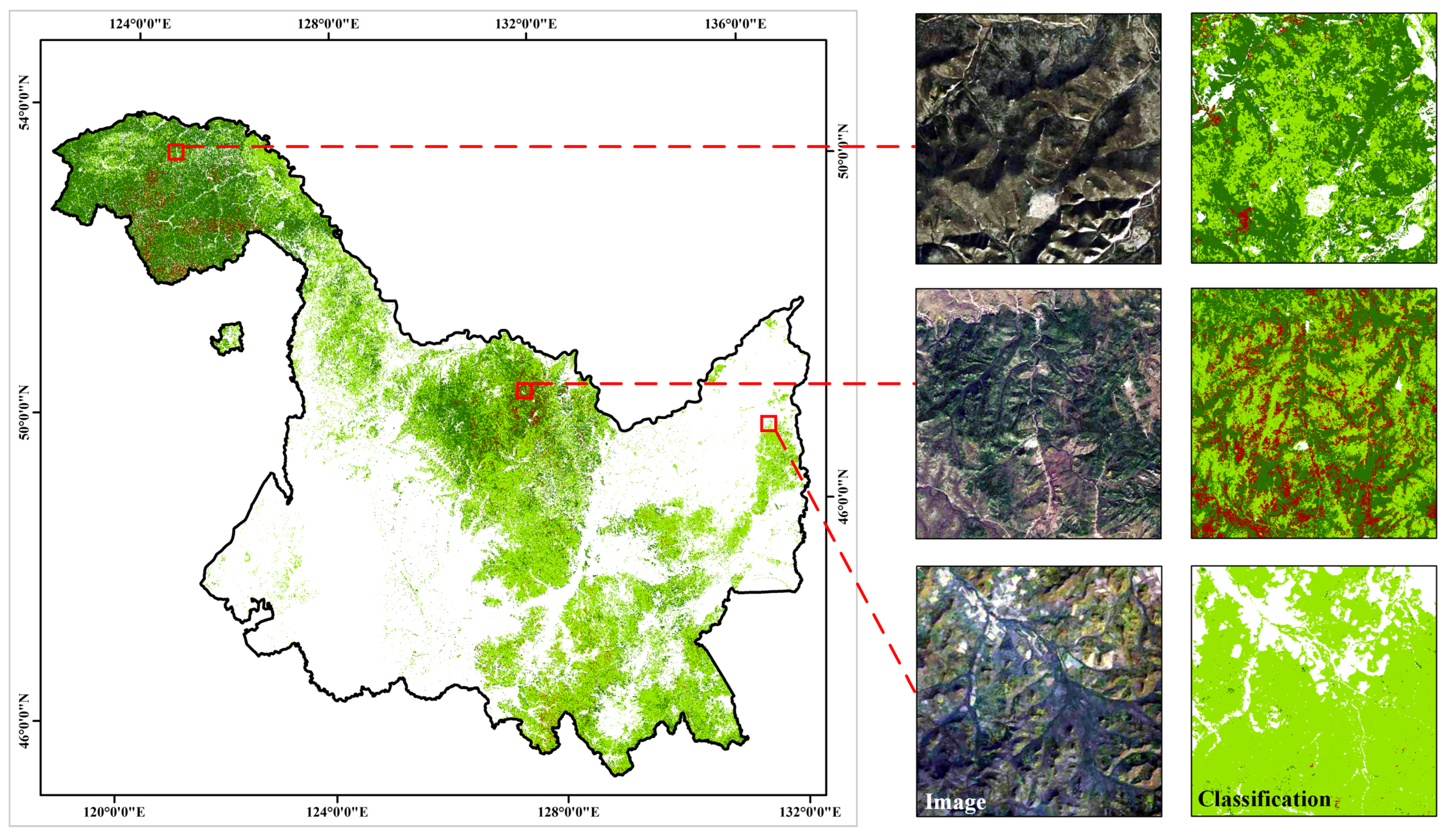
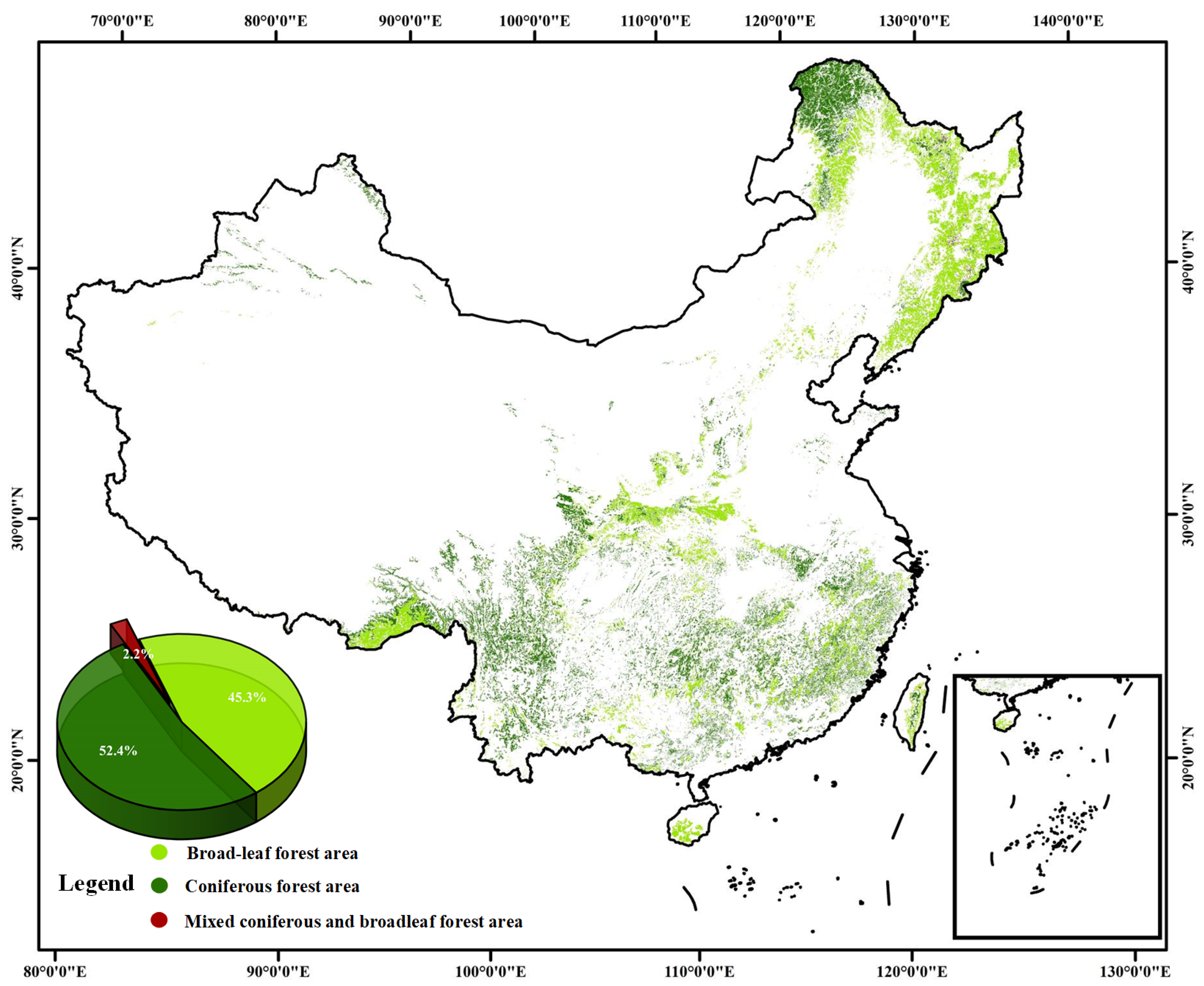
3.1. Distribution of China’s Forests in 2020

The forest distribution map of China in 2020 is shown in Figure 6, with an estimated forest area of 2,166,261.17 km 2 , which is very close to the area of 2,204,500 km 2 in the Ninth National Forest Inventory (2014–2018). The area of forests in each provincial area is presented in Table 3. Coniferous forests cover 1,127,294.42 km 2 , accounting for 52% of the total area; broad-leaf forests cover 981,690.98 km 2 , accounting for 45.3% of the total area; and mixed coniferous and broad-leaf forests cover 57,275.77 km 2 , accounting for 2.6% of the total area. By dividing China’s provinces into seven regions, it can be seen that the southwest region has the largest forest area and the northwest region has the smallest forest area. Heilongjiang, Inner Mongolia, Sichuan, and Yunnan provinces account for a larger proportion of the total area.

3.2. Accuracy Assessment

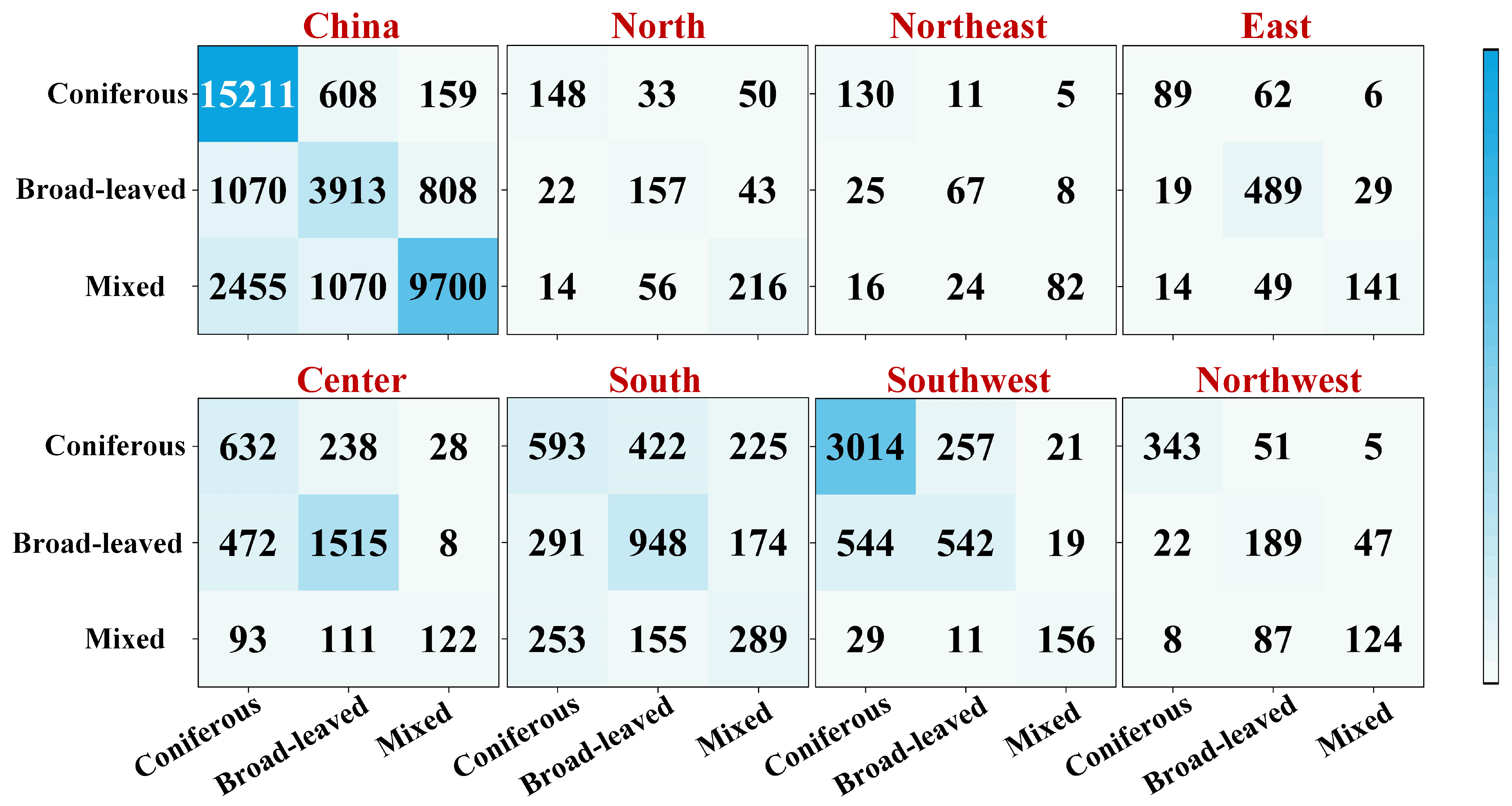
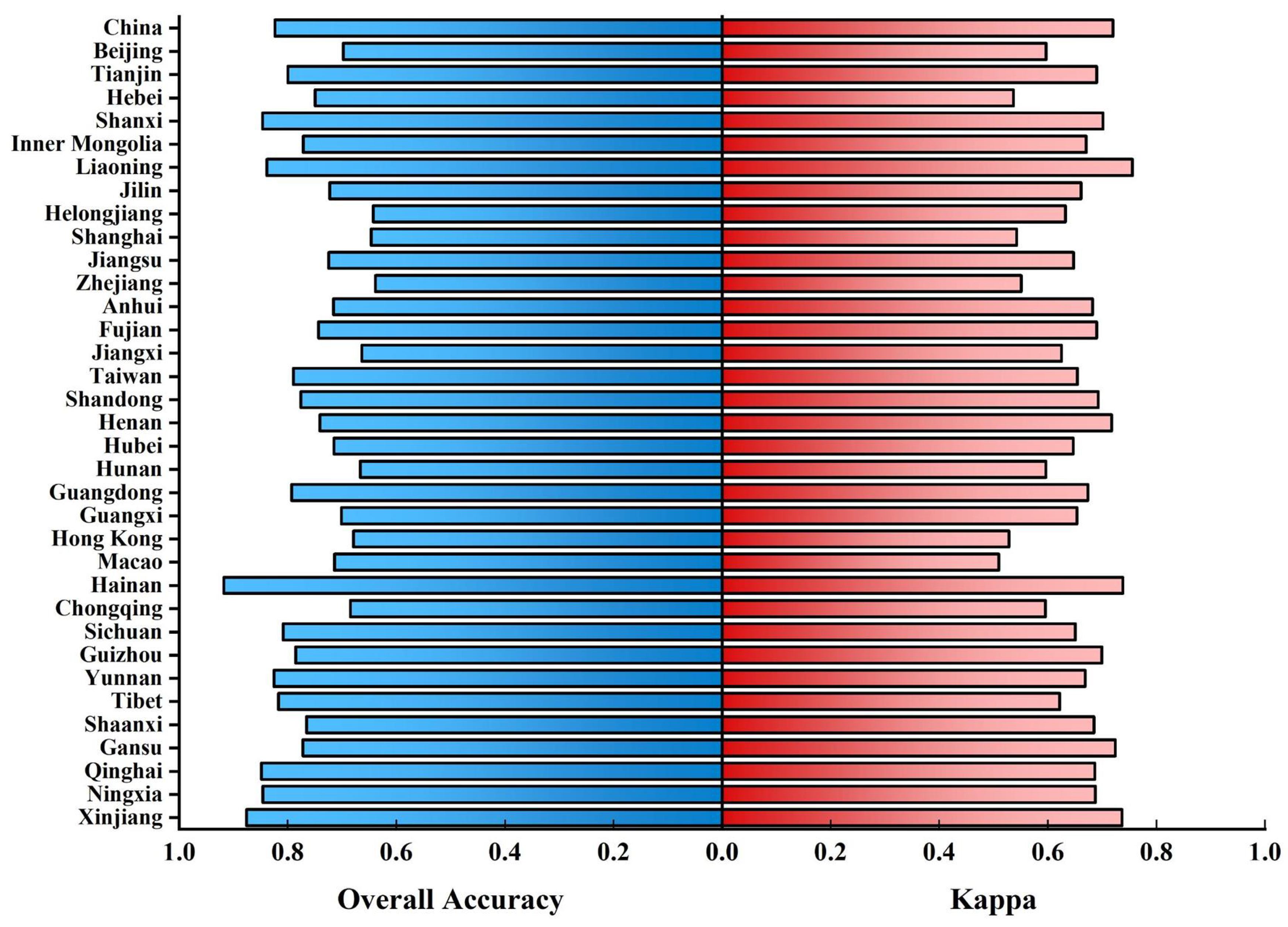
3.2.1. Comparison with Field Data

In order to show the forest classification results in detail, the ground data collected by Google Earth were used as an example, and three regions in Yunnan and Heilongjiang provinces were selected to demonstrate the results. In Figure 7 and Figure 8, the second column shows the ground data and the third column shows the classification results. The forest cover boundaries were accurately reflected, and the boundaries between coniferous forests, broad-leaf forests, and mixed coniferous and broad-leaf forests were clearly predicted. Overall, through the analysis of the validation samples and visualization results, we can see that the forest classification performed well and achieved acceptable results at the national and regional scales.
In this article, 93,567 data collected as the validation set were used to evaluate the generated maps, and seven regional and nationwide confusion matrices were obtained (Figure 9). Based on the nationwide confusion matrix, the overall accuracy (OA) achieved was 82.37% and the Kappa coefficient achieved was 0.72, indicating that the classification results were highly consistent with the validation sample. The overall accuracy and Kappa coefficient for each province are shown in Figure 10, where it can be seen that Hainan Province had the highest overall accuracy of 91.78% and Kappa coefficient of 0.74. Xinjiang Province was second to Hainan Province with an OA of 87.59% and a Kappa coefficient of 0.74. Since the dataset was collected manually, the distribution of the data collected from the forests in each province was uneven, and there was a difference between the number of training and validation samples. Moreover, the OA obtained was highly consistent with the validation sample. There were differences between the number and values of the OA and Kappa coefficients obtained. The OA values of most provinces were distributed around 78% and the Kappa coefficient values were distributed around 0.65. However, the OAs for Beijing, Heilongjiang, Shanghai, Zhejiang, Hunan, Hong Kong, and Jiangxi provinces were below 70%. This was caused by the training and validation samples, which were more urban in the region, and the forests were mainly distributed outside the cities and in places with smaller population distributions. So, it was more difficult to collect the dataset for this region with fewer samples.

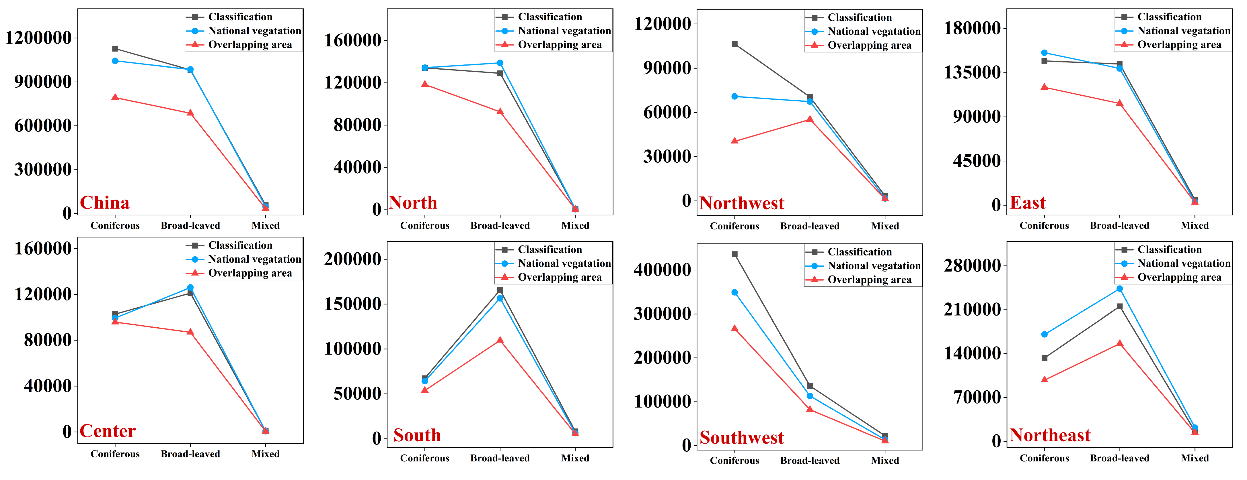
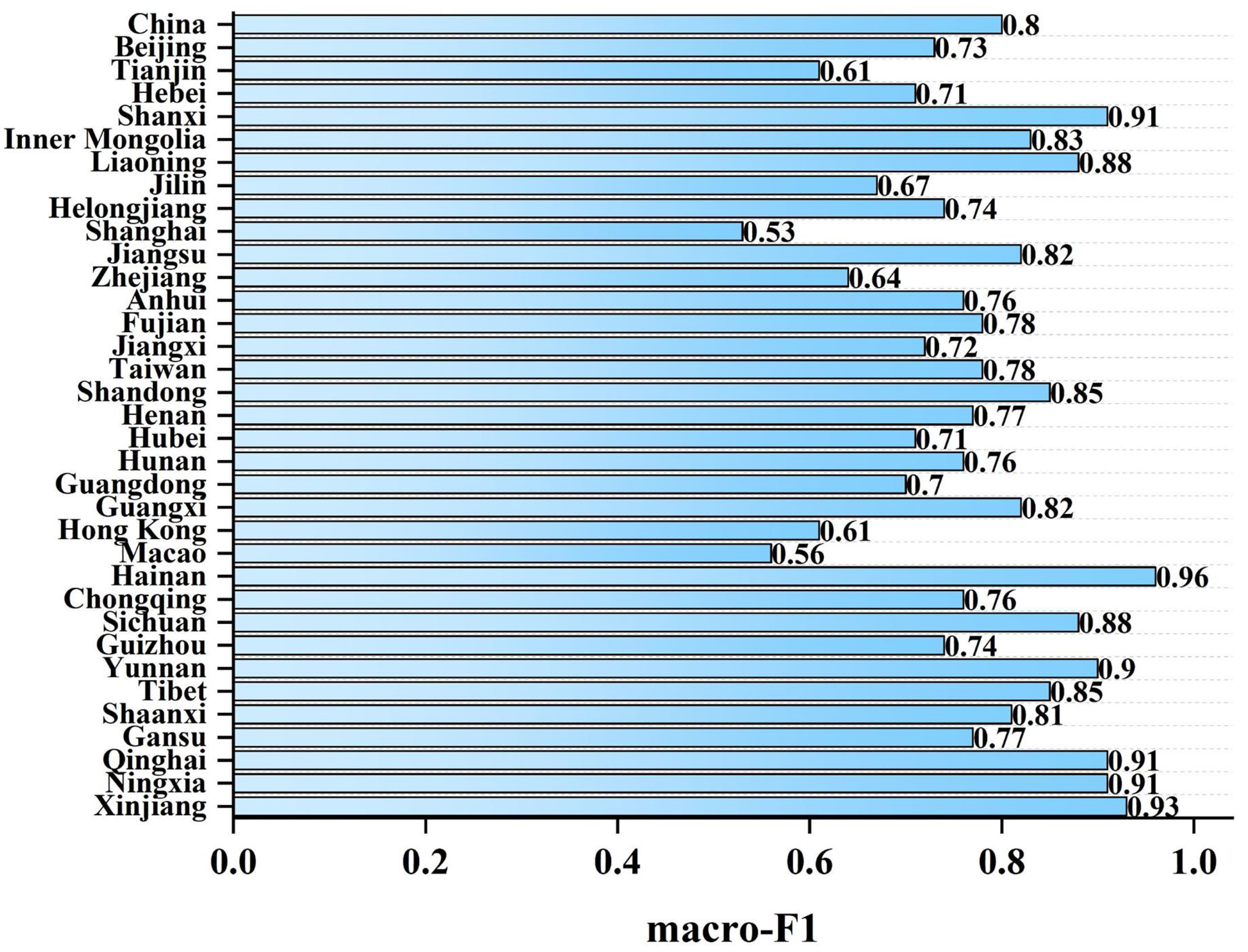
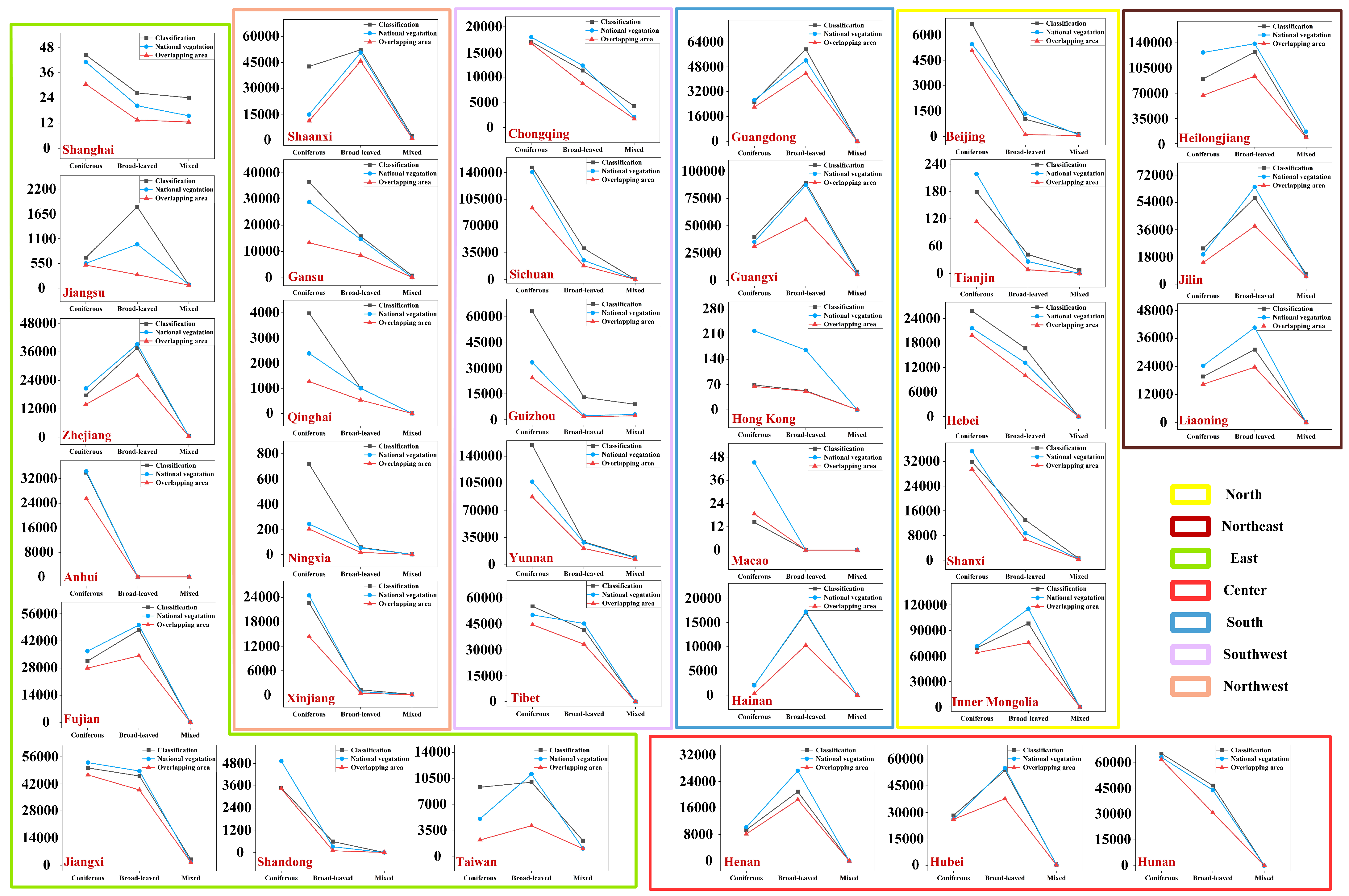
3.2.2. Comparison with National Vegetation Map

We performed pixel-level comparisons of the national vegetation map (2019) and the obtained classification maps. Since the resolution of the national vegetation map is 1,000,000 m, the classification map was resampled to a resolution of 1,000,000 m. The overlapping areas of coniferous, broad-leaf, and mixed coniferous and broad-leaf forests were identified, as shown in Figure 11. In the forest classification results we obtained, the total forest area was 2,166,261.17 km 2 , of which the coniferous forest area was 1,127,294.42 km 2 , the broad-leaf forest area was 981,690.98 km 2 , and the area of mixed coniferous and broad-leaf forest was 57,275.77 km 2 . In the national vegetation map, the forest area was 2,076,336.05 km 2 , of which the coniferous forest area was 1,043,690.98 km 2 . The overlapping area of the forest was 1,512,318.92 km 2 , of which the coniferous forest area was 792,603 km 2 , the broad-leaf forest area was 685,795.06 km 2 , and the area of mixed coniferous and broad-leaf forest was 33,839.9 km 2 . The total overlapping area accounted for 69.81% of the classification results, of which the overlapping area of coniferous forest accounted for 70.31% of the classification results, the overlapping area of broad-leaf forest accounted for 69.85% of the classification results, and the overlapping area of mixed coniferous and broad-leaf forest accounted for 59.08% of the classification results. The resulting data showed that the classification results of coniferous and broad-leaf forests were highly accurate, and the classification results of mixed coniferous and broad-leaf forests contained significant errors.

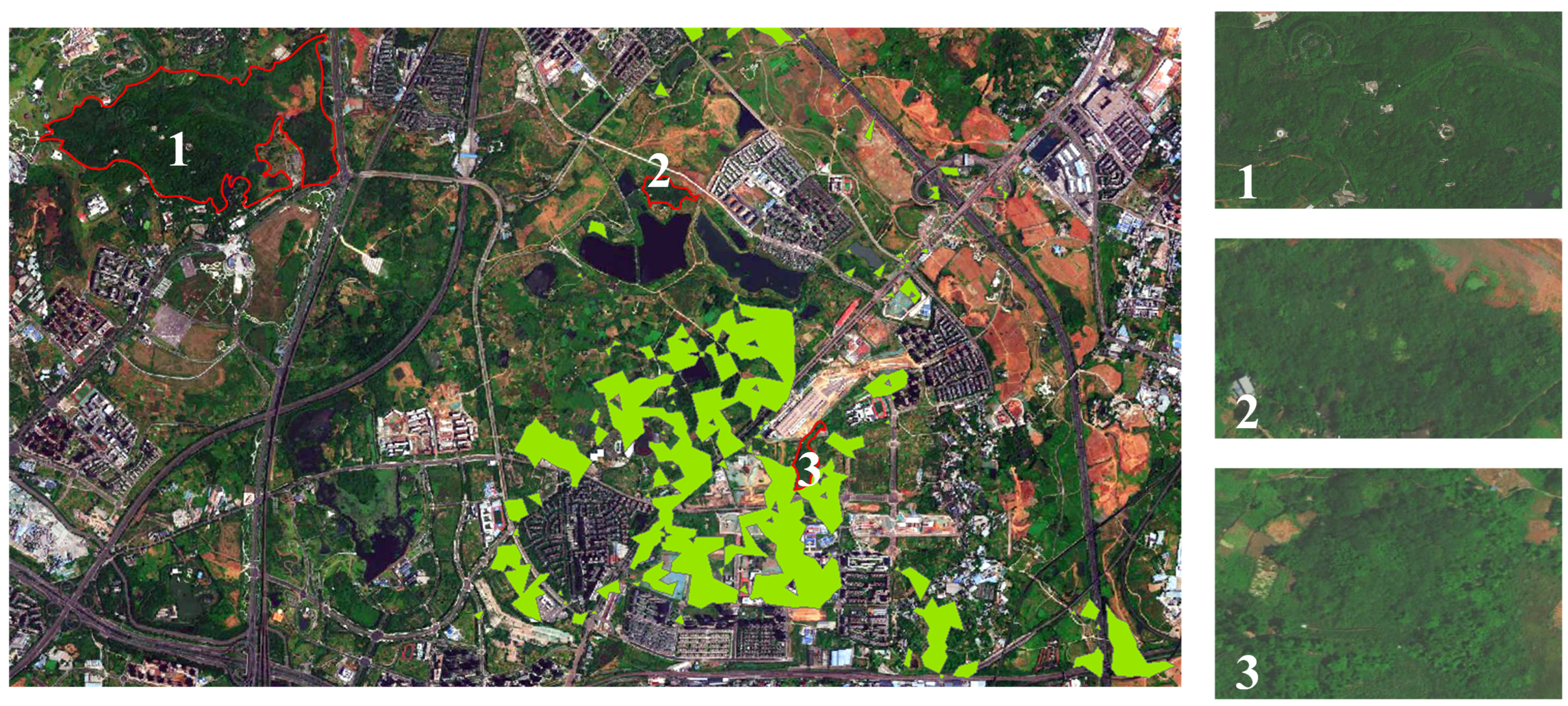
3.3. Uncertainties of the Forest Classification Forest Map

To assess and analyze the overall area of error in forest classification by region and province, we illustrated the distributions of the forest classification errors for the seven regions and 34 administrative districts using line graphs. Figure 12 shows the forest area for the whole country and the seven regions, where the black lines indicate the classification results of this study, the blue lines indicate those of the national vegetation map, and the red lines indicate the overlapping areas after the pixel-level comparison. As can be seen in the figure, the area of the classification results in each region was essentially the same as the forest area of the 30m resolution national vegetation map, but the coniferous forest area in the northwest region was larger. The overlapping area after the comparison consistently maintained a linear relationship with the classification results, which indicates that the classification results we obtained are statistically acceptable forest classification results for the whole country. However, in central and southern China, there were significant errors in the broad-leaf forest areas, and in northwestern China, there were significant errors in the coniferous forest areas. The overlapping areas in the other provinces were essentially the same as the classification results. The errors in Hong Kong, Macao, and Taiwan were mainly due to the small number of local samples. The samples we used were collected and uploaded manually, and the topographic data collected in some areas, such as cities with complex topography and high urban coverage, were also limited. Moreover, the longitudinal span of the Chinese region is large and the landforms are very different, which can easily lead to prediction errors. In northwest China, the land cover type is mainly barren, with sparse vegetation and bushes, resulting in a misclassification phenomenon. The relatively high elevation of the terrain in the region had a great impact on the data collection, leading to obvious errors in the prediction of coniferous forests. In eastern China, urbanization covers a large area, and the dataset used was relatively small and performed poorly for Jiangsu Province. In the north, northeast, southwest, and central regions of China, the performance of individual provincial administrations was fair and highly consistent with the survey data, as the forests in these regions are relatively similar and stable and not easily confused.
In conclusion, the statistical reliability of this study has been verified based on survey data from the 2019 national vegetation map. When examining the overall performance in the seven regions and 34 provincial administrations, the results show that the errors in this study are generally acceptable. The large differences between our classification maps and the national vegetation maps were mainly caused by the following reasons:
(1) Difficulties in the collection of local samples: Although the number of samples was large, the distribution of samples in each regional province was not balanced, resulting in different accuracies in each province. The local sample data also depended on the distribution of users using the software, e.g., in Hong Kong, Macao, and Taiwan, there were few users, as well as the image classification accuracy.
(2) Google Earth Engine imagery had uneven coverage: Figure 3 shows the spatial distribution of the number of image tiles captured by Sentinel-2 from 28 March 2017 to 30 December 2020 (our study period), where blue indicates that the amount of remote sensing image coverage in the region was high, and red indicates that the amount of remote sensing image coverage in the region was low. It can be seen in the figure that remote sensing image coverage was low in the southwest region, including Tibet and Sichuan, whereas in the north of China, remote sensing image coverage was higher. Although GEE is the best choice for obtaining high-resolution remote sensing images of the whole country, the uneven coverage of images can affect the uniformity of forest classification. The number of remote sensing images was relatively sparse, resulting in a decrease in classification accuracy in the region. Therefore, although the unevenness in the distribution of Sentinel-2 images still caused uncertainty in our classification results, the impact was minimized due to the rational use of image texture information and the combination of uniformly distributed Sentinel-1 image information.
(3) The change in the country’s forest area was rapid: According to the National Bureau of Statistics (NBS) [42], in the Eighth National Forest Inventory (NFI), the forest area of the country was 2,100,000 km 2 , whereas in the Ninth NFI, the forest area of the country was 2,204,500 km 2 , so the distribution and area of forests changed over time. The national vegetation map we used is from 2019, so spatial differences between that map and our classification map were inevitable.
(4) We analyzed the differences between the mapped areas and statistics for all provinces and presented them as line graphs. The results showed that the areas of broad-leaf forests mapped in the provinces of Jiangsu, Hebei, Yunnan, and Guizhou were significantly overestimated, and the areas of coniferous forests mapped in the provinces of Inner Mongolia, Heilongjiang, and Liaoning were significantly underestimated. This was due to the errors in the forest mask (GlobeLand30) land cover data, which under- or overestimated the forest areas in the northern and northwestern regions despite its high user accuracy (84.10% to 90.50%) and producer accuracy (92.10% to 93.90%). Many coniferous and broad-leaf forests in the provinces were not categorized as forests, resulting in underestimation, as shown in Figure 13.
(5) Resampling the classification map resulted in a loss of detailed information: The resolution of the national vegetation map is 1,000,000 m, whereas the resolution of our classification map is 30 m. When comparing the two maps, it was necessary to maintain the same resolution so we resampled the classification map to 1,000,000 m. The pixels were enlarged and shifted due to the process of resampling, resulting in the loss of some details, so the overlapping area was slightly smaller as a proportion of the total area when the two maps were compared. Therefore, when comparing the two maps with the national vegetation map, there were significant differences. Overall, differences in pixel-level comparisons between the two maps were unavoidable.

4. Discussion

In this study, we constructed a general framework for forest classification in China based on the spectral, textural, and structural features of multi-source remote sensing images and generated a 2020 classification map of coniferous forests, broad-leaf forests, and mixed coniferous and broad-leaf forests with the help of local samples. Random forest was used for feature importance selection, improving the efficiency and accuracy of classification, which is of great significance for forest management and conservation in China.
Open access to multi-source remote sensing images and cloud computing platforms has provided unprecedented convenience in the field of remote sensing. GEE, as a typical representative of cloud computing platforms, has powerful access and processing capabilities for satellite data, so it is often used for land-cover mapping on a large scale [43,44]. Traditional remote sensing data processing cannot operate on a large scale and the images need to be processed and spliced separately, which can lead to differences between different areas. This study relied on GEE’s advantage of storing a large amount of remote sensing data to perform mapping on a large scale in China. The data of Sentinel-1 and Sentinel-2 for the whole study area from 2017 to 2020, which comprised a substantial amount of data, were aggregated, effectively avoiding the problem of uneven color due to splicing and ensuring the quality of remote sensing data.
The local samples used in this study were from a phone application (LiVegetation), as well as the literature, which greatly improved the efficiency of data collection. The local samples provided the validation set and the training set, while the remote sensing images reflected the characteristics of the ground through different bands. The combination of the two improved the accuracy and efficiency of classification [45].
We calculated the texture features for 14 bands in Sentinel-2 and the structural features provided by Sentinel-1. In total, 254 bands were obtained. We used random forest for feature importance analysis for the bands and input them into the network in order of feature value size to obtain the training accuracy values from 1 band to 254 bands. The results showed that a large number of band features in the network can affect the operation speed and efficiency, resulting in redundancy. Therefore, in this study, the top 12 bands in terms of importance were selected to be input into the network for operation.
We compared the obtained classification map (30 m) with the national vegetation map (1,000,000 m) [46]. The resolution of the classification map is 30 m and it was resampled to a resolution of 1,000,000 m before the comparison. The results showed that the two maps overlapped on 69.8 % of the area of the classification map. We analyzed the sources of error and identified five possible causes: (a) The collected dataset was unevenly distributed across the country. (b) There were differences in the number of Sentinel-2 images that were unevenly distributed regionally within the time interval of the study. (c). The area of forests in the country changed rapidly. (d) The forest mask used (GlobeLand30) contained detailed errors and misclassification of forests. (e) Resampling led to a loss of detailed information due to the fact that the resolution of the national vegetation map was 1,000,000 m, resulting in a loss of some detailed information about the coordinates when mapping. It is worth mentioning that when our classification map is resampled, as the pixel point is zoomed in, the coordinates represented by that point will also change, resulting in errors in the subsequent comparison. Therefore, the area of error between the classification map and the national vegetation map is within acceptable limits.

5. Conclusions

In this study, we provide a reliable framework for large-scale forest classification by combining multi-source remote sensing images and local samples. With this framework, we generated a forest classification map of China in 2020 with a spatial resolution of 30 m. Sentinel-1 provided the structural features, and Sentinel-2 provided the spectral and textural features, offering discriminative features with different performances for forest classification in different regions. Meanwhile, the locally collected samples were used as mapping pipelines and as training and validation sets for training, which provided reliable data for this study. Two metrics, EVI and REPI, were constructed to add effective features. Integrating the bands of EVI, REPI, and S2 as inputs to the grayscale matrix yielded 252 texture features, which were combined with the structural features of S1 for feature importance selection. Considering the computational efficiency, the first 12 bands were selected as the final input. Finally, the features were trained and mapped using a random forest classifier. Our mapping results can provide accurate and reliable information on coniferous forests, broad-leaf forests, and mixed coniferous and broad-leaf forests in China, which is beneficial to the conservation and development of Chinese forests.

Author Contributions

Writing—original draft, X.Y. and Y.L.; Writing—review & editing, W.F.; Supervision, J.L., H.R., S.H. and M.L. All authors have read and agreed to the published version of the manuscript.

Funding

This work was supported by National Natural Science Foundation of China (Nos. 62201438, 62331019, 12005169); Basic Research Program of Natural Sciences of Shaanxi Province (No. 2021JC-23); Yulin Science and Technology Bureau Science and Technology Development Special Project (No. CXY-2020-094); Shaanxi Forestry Science and Technology Innovation Key Project (No. SXLK2022-02-8); and the Project of Shaanxi Federation of Social Sciences (No. 2022HZ1759).

Data Availability Statement

This study used Sentinel 1 SAR GRD, Sentinel 2A, and GobleLand30 data obtained from public domain resources. The data that support the findings of this study are available in the “EarthEngine Data Catalog ” on Google Earth Engine at https://developers.google.com/earth-engine/datasets/catalog/COPERNICUS_S1_GRD (accessed on 20 September 2023) and https://developers.google.com/earth-engine/datasets/catalog/COPERNICUS_S2_SR (accessed on 20 September 2023). All the vectors used in this project were obtained from http://datav.aliyun.com/portal/school/atlas/area_selector (accessed on 20 September 2023).

Conflicts of Interest

The authors declare that they have no known competing financial interests or personal relationships that could have influenced the work reported in this paper.

Appendix A

Appendix A.1

For more comprehensive insights, the delineation of the features can be found in Table A1.
Table A1. Overview of the bands of S2.
BandCenter Wavelength/nmResolution/mDescription
B144360Aerosols
B249010Blue
B356010Green
B466510Red
B570520Red Edge 1
B674020Red Edge 2
B778320Red Edge 3
B884210NIR
B8A86520Red Edge 4
B994060Water vapor
B11161020SWIR 1
B12219020SWIR 2
QA10 10
QA20 20
QA60 60Cloud Mask
AOT Aerosol Optical Thickness

Appendix A.2

As shown in Figure A1, the macro-F1 of China is 0.8. Shanxi, Yunnan, Qinghai, Ningxia, and Xinjiang all have higher classification accuracies, with macro-F1 values over 0.9, whereas Tianjin, Shanghai, Hong Kong, and Macao have lower macro-F1 values, which suggests that the framework’s prediction in this region is poor. Overall, the framework’s predictions are reliable at the national level.
Figure A1. Macro-F1 at the national and provincial levels.
Remotesensing 15 05026 g0a1

Appendix A.3

Figure A2 shows a detailed comparison of the 34 provinces in China. In the southern area of China, there are significant errors in the forest areas of Hong Kong and Macao; in the northwest area of China, there are significant errors in the coniferous forest areas of Qinghai Province and Ningxia; and in the eastern area of China, there are significant errors in the broad-leaf forest areas of Jiangsu Province and the forest areas of Taiwan.
Figure A2. The results for the 34 provinces in China were statistically compared with the data of the national vegetation map. The provinces in different geographic regions were represented by different wireframes.
Remotesensing 15 05026 g0a2

References

  1. Romijn, E.; Lantican, C.B.; Herold, M.; Lindquist, E.; Ochieng, R.; Wijaya, A.; Murdiyarso, D.; Verchot, L. Assessing change in national forest monitoring capacities of 99 tropical countries. For. Ecol. Manag. 2015, 352, 109–123. [Google Scholar] [CrossRef]
  2. Woodwell, G.M.; Whittaker, R.; Reiners, W.; Likens, G.E.; Delwiche, C.; Botkin, D. The Biota and the World Carbon Budget: The terrestrial biomass appears to be a net source of carbon dioxide for the atmosphere. Science 1978, 199, 141–146. [Google Scholar] [CrossRef] [PubMed]
  3. Martin, P.A.; Newton, A.C.; Bullock, J.M. Carbon pools recover more quickly than plant biodiversity in tropical secondary forests. Proc. R. Soc. B Biol. Sci. 2013, 280, 20132236. [Google Scholar] [CrossRef]
  4. Huang, W.; Liu, J.; Wang, Y.P.; Zhou, G.; Han, T.; Li, Y. Increasing phosphorus limitation along three successional forests in southern China. Plant Soil 2013, 364, 181–191. [Google Scholar]
  5. Xiang, W.; Liu, S.; Lei, X.; Frank, S.C.; Tian, D.; Wang, G.; Deng, X. Secondary forest floristic composition, structure, and spatial pattern in subtropical China. J. For. Res. 2013, 18, 111–120. [Google Scholar]
  6. Zhou, G.; Peng, C.; Li, Y.; Liu, S.; Zhang, Q.; Tang, X.; Liu, J.; Yan, J.; Zhang, D.; Chu, G. A climate change-induced threat to the ecological resilience of a subtropical monsoon evergreen broad-leaved forest in Southern China. Glob. Chang. Biol. 2013, 19, 1197–1210. [Google Scholar]
  7. Cao, S.; Chen, L.; Shankman, D.; Wang, C.; Wang, X.; Zhang, H. Excessive reliance on afforestation in China’s arid and semi-arid regions: Lessons in ecological restoration. Earth-Sci. Rev. 2011, 104, 240–245. [Google Scholar]
  8. Liu, J.; Li, S.; Ouyang, Z.; Tam, C.; Chen, X. Ecological and socioeconomic effects of China’s policies for ecosystem services. Proc. Natl. Acad. Sci. USA 2008, 105, 9477–9482. [Google Scholar]
  9. Paquette, A.; Messier, C. The role of plantations in managing the world’s forests in the Anthropocene. Front. Ecol. Environ. 2010, 8, 27–34. [Google Scholar]
  10. Farooq, T.H.; Shakoor, A.; Wu, X.; Li, Y.; Rashid, M.H.U.; Zhang, X.; Gilani, M.M.; Kumar, U.; Chen, X.; Yan, W. Perspectives of plantation forests in the sustainable forest development of China. iForest-Biogeosci. For. 2021, 14, 166–174. [Google Scholar] [CrossRef]
  11. Gorelick, N.; Hancher, M.; Dixon, M.; Ilyushchenko, S.; Thau, D.; Moore, R. Google Earth Engine: Planetary-scale geospatial analysis for everyone. Remote Sens. Environ. 2017, 202, 18–27. [Google Scholar] [CrossRef]
  12. Bowditch, E.; Santopuoli, G.; Binder, F.; Del Rio, M.; La Porta, N.; Kluvankova, T.; Lesinski, J.; Motta, R.; Pach, M.; Panzacchi, P.; et al. What is Climate-Smart Forestry? A definition from a multinational collaborative process focused on mountain regions of Europe. Ecosyst. Serv. 2020, 43, 101113. [Google Scholar]
  13. Bowditch, E.; Santopuoli, G.; Neroj, B.; Svetlik, J.; Tominlson, M.; Pohl, V.; Avdagić, A.; del Rio, M.; Zlatanov, T.; Maria, H.; et al. Application of climate-smart forestry–Forest manager response to the relevance of European definition and indicators. Trees For. People 2022, 9, 100313. [Google Scholar] [CrossRef]
  14. Klerkx, L.; Jakku, E.; Labarthe, P. A review of social science on digital agriculture, smart farming and agriculture 4.0: New contributions and a future research agenda. NJAS-Wagening. J. Life Sci. 2019, 90, 100315. [Google Scholar]
  15. Moore, M.M.; Bauer, M.E. Classification of forest vegetation in north-central Minnesota using Landsat Multispectral Scanner and Thematic Mapper data. For. Sci. 1990, 36, 330–342. [Google Scholar]
  16. Walsh, S.J. Coniferous tree species mapping using Landsat data. Remote Sens. Environ. 1980, 9, 11–26. [Google Scholar]
  17. Mallinis, G.; Koutsias, N.; Tsakiri-Strati, M.; Karteris, M. Object-based classification using Quickbird imagery for delineating forest vegetation polygons in a Mediterranean test site. ISPRS J. Photogramm. Remote Sens. 2008, 63, 237–250. [Google Scholar]
  18. Zhang, C.; Qiu, F. Mapping individual tree species in an urban forest using airborne lidar data and hyperspectral imagery. Photogramm. Eng. Remote Sens. 2012, 78, 1079–1087. [Google Scholar]
  19. Feng, W.; Dauphin, G.; Huang, W.; Quan, Y.; Bao, W.; Wu, M.; Li, Q. Dynamic synthetic minority over-sampling technique-based rotation forest for the classification of imbalanced hyperspectral data. IEEE J. Sel. Top. Appl. Earth Obs. Remote Sens. 2019, 12, 2159–2169. [Google Scholar] [CrossRef]
  20. Pant, P.; Heikkinen, V.; Hovi, A.; Korpela, I.; Hauta-Kasari, M.; Tokola, T. Evaluation of simulated bands in airborne optical sensors for tree species identification. Remote Sens. Environ. 2013, 138, 27–37. [Google Scholar]
  21. Descals, A.; Wich, S.; Meijaard, E.; Gaveau, D.L.; Peedell, S.; Szantoi, Z. High-resolution global map of smallholder and industrial closed-canopy oil palm plantations. Earth Syst. Sci. Data 2021, 13, 1211–1231. [Google Scholar]
  22. Zhao, Y.; Zhu, W.; Wei, P.; Fang, P.; Zhang, X.; Yan, N.; Liu, W.; Zhao, H.; Wu, Q. Classification of Zambian grasslands using random forest feature importance selection during the optimal phenological period. Ecol. Indic. 2022, 135, 108529. [Google Scholar]
  23. Nguyen, Q.P.; Lim, K.W.; Divakaran, D.M.; Low, K.H.; Chan, M.C. GEE: A gradient-based explainable variational autoencoder for network anomaly detection. In Proceedings of the 2019 IEEE Conference on Communications and Network Security (CNS), Washington, DC, USA, 10–12 June 2019; IEEE: Piscataway, NJ, USA, 2019; pp. 91–99. [Google Scholar]
  24. Torres, R.; Snoeij, P.; Geudtner, D.; Bibby, D.; Davidson, M.; Attema, E.; Potin, P.; Rommen, B.; Floury, N.; Brown, M.; et al. GMES Sentinel-1 mission. Remote Sens. Environ. 2012, 120, 9–24. [Google Scholar] [CrossRef]
  25. Vollrath, A.; Mullissa, A.; Reiche, J. Angular-based radiometric slope correction for Sentinel-1 on google earth engine. Remote Sens. 2020, 12, 1867. [Google Scholar]
  26. Phiri, D.; Simwanda, M.; Salekin, S.; Nyirenda, V.R.; Murayama, Y.; Ranagalage, M. Sentinel-2 data for land cover/use mapping: A review. Remote Sens. 2020, 12, 2291. [Google Scholar]
  27. Cheng, K.; Su, Y.; Guan, H.; Tao, S.; Ren, Y.; Hu, T.; Ma, K.; Tang, Y.; Guo, Q. Mapping China’s planted forests using high resolution imagery and massive amounts of crowdsourced samples. ISPRS J. Photogramm. Remote Sens. 2023, 196, 356–371. [Google Scholar]
  28. Chen, J.; Chen, J.; Liao, A.; Cao, X.; Chen, L.; Chen, X.; He, C.; Han, G.; Peng, S.; Lu, M.; et al. Global land cover mapping at 30 m resolution: A POK-based operational approach. ISPRS J. Photogramm. Remote Sens. 2015, 103, 7–27. [Google Scholar]
  29. Torbick, N.; Ledoux, L.; Salas, W.; Zhao, M. Regional mapping of plantation extent using multisensor imagery. Remote Sens. 2016, 8, 236. [Google Scholar] [CrossRef]
  30. Testa, S.; Soudani, K.; Boschetti, L.; Mondino, E.B. MODIS-derived EVI, NDVI and WDRVI time series to estimate phenological metrics in French deciduous forests. Int. J. Appl. Earth Obs. Geoinf. 2018, 64, 132–144. [Google Scholar]
  31. Frampton, W.J.; Dash, J.; Watmough, G.; Milton, E.J. Evaluating the capabilities of Sentinel-2 for quantitative estimation of biophysical variables in vegetation. ISPRS J. Photogramm. Remote Sens. 2013, 82, 83–92. [Google Scholar] [CrossRef]
  32. Liang, J.; Zheng, Z.; Xia, S.; Zhang, X.; Tang, Y. Crop recognition and evaluationusing red edge features of GF-6 satellite. Yaogan Xuebao/J. Remote Sens. 2020, 24, 1168–1179. [Google Scholar] [CrossRef]
  33. Hong, D.; Yokoya, N.; Chanussot, J.; Zhu, X.X. An augmented linear mixing model to address spectral variability for hyperspectral unmixing. IEEE Trans. Image Process. 2018, 28, 1923–1938. [Google Scholar] [CrossRef]
  34. Tassi, A.; Vizzari, M. Object-oriented lulc classification in google earth engine combining snic, glcm, and machine learning algorithms. Remote Sens. 2020, 12, 3776. [Google Scholar] [CrossRef]
  35. Haralick, R.M.; Shanmugam, K.; Dinstein, I.H. Textural features for image classification. IEEE Trans. Syst. Man Cybern. 1973, 610–621. [Google Scholar] [CrossRef]
  36. Conners, R.W.; Trivedi, M.M.; Harlow, C.A. Segmentation of a high-resolution urban scene using texture operators. Comput. Vision Graph. Image Process. 1984, 25, 273–310. [Google Scholar]
  37. Wang, S.; Feng, W.; Quan, Y.; Li, Q.; Dauphin, G.; Huang, W.; Li, J.; Xing, M. A heterogeneous double ensemble algorithm for soybean planting area extraction in Google Earth Engine. Comput. Electron. Agric. 2022, 197, 106955. [Google Scholar] [CrossRef]
  38. Feng, W.; Dauphin, G.; Huang, W.; Quan, Y.; Liao, W. New margin-based subsampling iterative technique in modified random forests for classification. Knowl.-Based Syst. 2019, 182, 104845. [Google Scholar]
  39. Breiman, L. Random forests. Mach. Learn. 2001, 45, 5–32. [Google Scholar] [CrossRef]
  40. Feng, W.; Quan, Y.; Dauphin, G.; Li, Q.; Gao, L.; Huang, W.; Xia, J.; Zhu, W.; Xing, M. Semi-supervised rotation forest based on ensemble margin theory for the classification of hyperspectral image with limited training data. Inf. Sci. 2021, 575, 611–638. [Google Scholar]
  41. Oreti, L.; Giuliarelli, D.; Tomao, A.; Barbati, A. Object oriented classification for mapping mixed and pure forest stands using very-high resolution imagery. Remote Sens. 2021, 13, 2508. [Google Scholar]
  42. Su, Y.; Guo, Q.; Hu, T.; Guan, H.; Jin, S.; An, S.; Chen, X.; Guo, K.; Hao, Z.; Hu, Y.; et al. An updated vegetation map of China (1: 1000000). Sci. Bull. 2020, 65, 1125–1136. [Google Scholar] [CrossRef] [PubMed]
  43. Dong, J.; Xiao, X.; Menarguez, M.A.; Zhang, G.; Qin, Y.; Thau, D.; Biradar, C.; Moore III, B. Mapping paddy rice planting area in northeastern Asia with Landsat 8 images, phenology-based algorithm and Google Earth Engine. Remote Sens. Environ. 2016, 185, 142–154. [Google Scholar] [CrossRef] [PubMed]
  44. Chen, B.; Xiao, X.; Li, X.; Pan, L.; Doughty, R.; Ma, J.; Dong, J.; Qin, Y.; Zhao, B.; Wu, Z.; et al. A mangrove forest map of China in 2015: Analysis of time series Landsat 7/8 and Sentinel-1A imagery in Google Earth Engine cloud computing platform. ISPRS J. Photogramm. Remote Sens. 2017, 131, 104–120. [Google Scholar] [CrossRef]
  45. Teluguntla, P.; Thenkabail, P.S.; Oliphant, A.; Xiong, J.; Gumma, M.K.; Congalton, R.G.; Yadav, K.; Huete, A. A 30-m landsat-derived cropland extent product of Australia and China using random forest machine learning algorithm on Google Earth Engine cloud computing platform. ISPRS J. Photogramm. Remote Sens. 2018, 144, 325–340. [Google Scholar] [CrossRef]
  46. Li, Z.; He, W.; Cheng, M.; Hu, J.; Yang, G.; Zhang, H. SinoLC-1: The first 1-meter resolution national-scale land-cover map of China created with the deep learning framework and open-access data. Earth Syst. Sci. Data Discuss. 2023, 2023, 1–38. [Google Scholar]
Figure 1. The methodological workflow implemented in GEE.
Remotesensing 15 05026 g001
Figure 2. Illustration of the regional divisions and the distribution of forest samples.
Remotesensing 15 05026 g002
Figure 3. Number of Sentinel-2 scenes over China during the study period from 28 March 2017 to 30 December 2020. The color ranges from blue to red, indicating fewer scenes. The darker the color, the fewer scenes in the area.
Remotesensing 15 05026 g003
Figure 4. Evaluation of the importance of the spectral, textural, and structural features within seven regions. Blue represents the original band and green represents the texture features after GLCM.
Remotesensing 15 05026 g004
Figure 5. As the input of 254 bands increases, the accuracy follows the curve of the frame.
Remotesensing 15 05026 g005
Figure 6. Map of classification of coniferous and broad-leaf forests in China.
Remotesensing 15 05026 g006
Figure 7. Illustration of Yunnan province. The remote sensing images in the figure are from © Google Earth 2020.
Remotesensing 15 05026 g007
Figure 8. Illustration of Heilongjiang province. The remote sensing images in the figure are from © Google Earth 2020.
Remotesensing 15 05026 g008
Figure 9. Confusion matrix for the classification of coniferous, broad-leaf, and mixed coniferous and broad-leaf forests at the national and provincial levels in China.
Remotesensing 15 05026 g009
Figure 10. Overall accuracy and Kappa coefficients at the national and provincial levels.
Remotesensing 15 05026 g010
Figure 11. Overlapping areas between the map generated in this study (2020) and the national vegetation map (2019).
Remotesensing 15 05026 g011
Figure 12. Statistical comparison of 7 regional and national vegetation maps in China. In each plot, the horizontal coordinate represents the forest type, and the vertical coordinate represents the area covered. The black line shows the area of the study, the blue line shows the area of the national vegetation map, and the red line shows the overlapping area of the two.
Remotesensing 15 05026 g012
Figure 13. Example of forest area underestimation in GlobeLand30 data. The remote sensing images in the figure are from © Google Earth 2020.
Remotesensing 15 05026 g013
Table 1. Statistics of samples by region.
RegionProvinceNumber of SamplesTotal
NorthBeijing49720,123
Tianjin45
Hebei1346
Shanxi15,006
Inner Mongolia3229
NortheastLiaoning588018,326
Jilin3904
Heilongjiang8542
EastShanghai128185,861
Jiangsu3535
Zhejiang11,459
Anhui4936
Fujian21,804
Jiangxi18,742
Taiwan1823
Shandong22,381
CenterHenan387345,681
Hubei16,443
Hunan25,365
SouthGuangdong255826,680
Guangxi23,844
Hong Kong30
Macao7
Hainan241
SouthwestChongqing13,63575,381
Sichuan41,666
Guizhou6071
Yunnan11,478
Tibet2531
NorthwestShaanxi17,82539,738
Gansu15,519
Qinghai1083
Ningxia551
Xinjiang4760
311,890
Table 2. Characteristic importance analyses of 254 bands across China and ranked in descending order of importance. The first 18 of these bands are shown below.
BandImportanceBandImportanceBandImportance
B1_savg18.958B9_savg15.711B3_prom15.226
B2_savg17.409VV15.678B5_dvar14.991
B1_shade17.241B8A_savg15.550B1_idm14.853
B7_savg16.934REPI_savg15.435EVI_shade14.839
B5_savg16.044VH15.389B6_idm14.741
EVI_savg15.912B11_savg15.373B5_shade14.617
Table 3. Area of the three types of forests in each province.
RegionProvinceConiferous/km 2 Broad-Leaf/km 2 Mixed/km 2 Total//km 2 Percent/%
NorthBeijing6,661.911,018.35166.297,846.550.36
Tianjin178.2241.267.5226.980.01
Hebei25,865.7716,725.321.0542,592.141.97
Shanxi31,775.1813,045.02593.3445,413.542.10
Inner Mongolia69,728.8198,247.586.7167,983.097.75
264,062.312.19
NortheastLiaoning19,660.4131,282.3638.4950,981.262.35
Jilin23,627.0156,882.87,011.0287,520.834.04
Heilongjiang89,905.14127,198.538,996.01226,099.6810.44
364,601.7716.83
EastShanghai44.4726.3624.0994.920.00
Jiangsu678.61,806.6376.822,562.050.12
Zhejiang17,637.1637,665.23601.855,904.192.58
Anhui34,004.675.720.0934,013.481.57
Fujian31,548.9547,649.9615.779,214.613.66
Jiangxi50,174.0646,016.372919.9499,110.374.58
Taiwan9,303.479,977.722,092.0721,373.260.99
Shandong3,470.8590.320.124,061.240.19
296,334.1213.68
CenterHenan9,415.1820,9216.4230,342.61.40
Hubei28,330.953,717.53697.4782,745.93.82
Hunan65,070.7446,516.89164.52111,752.155.16
224,840.6510.38
SouthGuangdong25,592.2959,261.5843.984,897.773.92
Guangxi39,644.7689,432.198,058.34137,135.296.33
Hong Kong68.8352.640121.470.01
Macao14.320014.310.00
Hainan2,056.517,033.53019,090.030.88
241,258.8711.14
SouthwestChongqing17,029.2111,295.874,219.5532,544.631.50
Sichuan146,670.3140,738.0281.56187,489.898.65
Guizhou62,969.3813,024.968,981.3784,975.713.92
Yunnan154,402.0429,265.639,060.16192,727.838.90
Tibet55,258.3841,689.7120.6996,968.784.48
594,706.8427.45
NorthwestShaanxi42,740.6452,406.422,406.0997,553.154.50
Gansu36,42815,813.78829.2953,071.072.45
Qinghai3,978.61,002.570.024,981.190.23
Ningxia716.6655.990.08772.730.04
Xinjiang22,640.061,283.14155.2824,078.481.11
180,456.628.33
2,166,261.2100
Disclaimer/Publisher’s Note: The statements, opinions and data contained in all publications are solely those of the individual author(s) and contributor(s) and not of MDPI and/or the editor(s). MDPI and/or the editor(s) disclaim responsibility for any injury to people or property resulting from any ideas, methods, instructions or products referred to in the content.

