
A New Remote Sensing Desert Vegetation Detection Index


1
School of Civil Engineering and Geomatics, Shandong University of Technology, Zibo 255049, China
2
State Key Laboratory of Resources and Environmental Information System, Institute of Geographical Sciences and Natural Resources Research, Chinese Academy of Sciences, Beijing 100101, China
3
Hunan Provincial Key Laboratory of Geo-Information Engineering in Surveying, Mapping and Remote Sensing, Hunan University of Science and Technology, Xiangtan 411201, China
4
Academy of Forestry Inventory and Planning, National Forestry and Grassland Administration, Beijing 100714, China
5
Shandong Zhengyuan Digital City Construction Co., Ltd., Yantai 264670, China
*
Author to whom correspondence should be addressed.
Remote Sens. 2023, 15(24), 5742; https://0-doi-org.brum.beds.ac.uk/10.3390/rs15245742
Submission received: 11 October 2023
/
Revised: 6 December 2023
/
Accepted: 11 December 2023
/
Published: 15 December 2023
(This article belongs to the Special Issue Land Degradation Assessment with Earth Observation (Second Edition))
Abstract
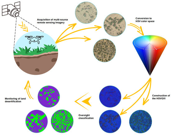
:Land desertification is a key environmental problem in China, especially in Northwest China, where it seriously affects the sustainable development of natural resources. In this paper, we combine high-resolution satellite remote sensing images and UAV (unmanned aerial vehicle) visible light images to extract desert vegetation data and quickly locate and accurately monitor land desertification in relevant areas according to changes in vegetation coverage. Due to the strong light and dry climate of deserts in Northwest China, which results in deeper vegetation shadow texture and mostly dry shrubs with fewer stems and leaves, the accuracy of the vegetation index commonly used in visible remote sensing image classification is not able to meet the requirements for monitoring and evaluating land desertification. For this reason, in this paper, we took the Hangjin Banner in Bayannur as an example and constructed a new vegetation index, the HSVGVI (hue–saturation–value green enhancement vegetation index), based on the HSV (hue–saturation–value) color space using channel enhancement that can improve the extraction accuracy of desert vegetation and reduce misclassification. In addition, in order to further test the extraction accuracy, samples of densely vegetated and multi-shaded areas were divided in the study area according to the accuracy-influencing factors. At the same time, the HSVGVI was compared with the vegetation indices EXG (excess green index), RGBVI (red–green–blue vegetation index), MGRVI (modified green–red vegetation index), NGBDI (normalized green–red discrepancy index), and VDVI (visible-band discrepancy vegetation index) constructed based on the RGB (red–green–blue) color space. The experimental results show that the extraction accuracy of the EXG and other vegetation indices constructed in RGB color space can only reach 70%, while the extraction accuracy of the HSVGVI can reach more than 95%. In summary, the HSVGVI proposed in this paper can better realize the extraction of desert vegetation data and can provide a reliable technical tool for monitoring and evaluating land desertification.
1. Introduction
Land desertification is a major ecological problem facing arid and semi-arid regions worldwide [1]. It often occurs in mid-latitude regions, directly or indirectly affects more than 100 countries worldwide, involves more than one billion people, causes losses of up to USD 10 billion per year, and is ranked as one of the most serious environmental and social problems in the world [2,3]. According to the statistics released by the United Nations regarding land desertification, the problem of land desertification faced by China is particularly serious, which is mainly concentrated in the western and northern regions of China, severely restricting local economic development and placing great pressure upon the grassland ecological environment [4]. Among these regions, the Hangjin Banner in the Inner Mongolia Autonomous Region is a key area for the prevention and control of land desertification disasters in China [5]. The Hangjin Banner is rich in vegetation resources, which are mainly dominated by tree species with strong drought tolerance and low shrubs. The topography of the region mainly consists of hills and plateaus, so there are high elevations, complex terrain, and a wide range of topography [6]. Therefore, when monitoring land desertification in this region, one often faces the problems of low efficiency and high labor costs, which are not conducive to the prevention and management of land desertification.
With the rapid development of remote sensing technology, UAV remote sensing technology has become more and more mature, which is widely used in remote sensing vegetation classification research by virtue of its low cost and high accuracy in obtaining remote sensing images [7]. Scholars at home and abroad have utilized UAV remote sensing technology to classify urban vegetation [8], grassland vegetation [9,10], forest vegetation [11,12], wetland vegetation [13], crops [14,15], and other vegetation, and all of them have achieved good results. UAV remote sensing technology has also gradually been combined with geological exploration and forestry resource surveys, and compared with the traditional field survey method, it can not only monitor the distribution of vegetation but also accurately identify the growth of vegetation, which has become an efficient and accurate means of remote monitoring [16]. In the future, UAV remote sensing technology will also be used for the monitoring of farmland, the assessment of crop growth, and the monitoring of other natural disasters, as well as in other applications [17]. Meanwhile, high-resolution satellite remote sensing images continue to surpass the meter and sub-meter accuracy benchmarks [18]. Among the existing technologies, high-resolution satellite remote-sensing images have the ability to dynamically monitor land desertification on a large scale [19]. High-resolution satellite remote sensing images are used to establish vegetation cover models in a study area and analyze the areas that have undergone or are about to face land desertification disasters [20,21]. According to the relationship between vegetation coverage and desertification degree, the degree of desertification is graded, with FVC > 0.8 indicating non-desertification (potential desertification); 0.6 < FVC ≤ 0.8 refers to mild desertification; 0.4 < FVC ≤ 0.6 is moderate desertification; 0.2 < FVC ≤ 0.4 refers to severe desertification; and FVC ≤ 0.2 indicates extremely severe desertification [22]. Therefore, areas with vegetation coverage (FVC) less than 0.3 are designated as key monitoring areas for land desertification issues. Subsequently, visible remote sensing images from drones in a study area are utilized to extract desert vegetation information by processing the images, which are used to evaluate the degree of land desertification in the area [23,24]. Therefore, extracting desert vegetation data through a combination of multi-source remote sensing data based on high-resolution satellite remote sensing images and UAV visible remote sensing images can help us dynamically monitor and combat land desertification, improve monitoring efficiency, and significantly reduce the workload of monitoring personnel.
In the process of extracting vegetation information, constructing a vegetation index is an indispensable and important technical means for extracting vegetation coverage and monitoring land desertification via UAV visible light images. Wang Xiaoqin [25] and others proposed a new vegetation index model, the VDVI, by combining the vegetation and non-vegetation characteristics of UAV visible images and drawing on the principle of NDVI construction; the extraction accuracy of this index can reach more than 90%. Li Dongsheng [26] and others validated both the EXG and VDVI, and their accuracies can reach more than 90%, which indicates that these indices are basically able to accurately extract vegetation information. Bareth G [27] and others proposed the RGBVI, which is applied to the extraction of vegetation cover in agricultural fields, and its accuracy can reach more than 85%. However, due to the complex and harsh environment in deserts, it is difficult to adapt the vegetation index commonly used in cities and villages to the extraction of desert vegetation. In particular, in the desert area of Northwest China, due to the strong light and dry climate, the shadow texture produced by a tall tree canopy shows a darker color. Vegetation in desert areas has fewer stems and leaves and is mostly dry shrubs [28]. Therefore, the vegetation index model constructed using the RGB color space is often limited by the shadow texture of vegetation when extracting vegetation data, which causes the problem of misclassification and leads to large errors [29]. This is due to the fact that visible images are based on RGB color space, in which the correlation between R, G, and B channels is strong and not easy to analyze quantitatively, so much so that the classification results cannot provide accurate data for land desertification monitoring [30]. For complex desert environments, it is crucial to ensure the accuracy of vegetation data extraction and the applicability of the vegetation index model [31,32,33]. Since the HSV color space model focuses more on color representation, and this model is less affected by light, the H-value varies greatly between different feature types and is also relatively consistent with the subjective perception of color by the human eye. It is able to capture the fine green vegetation well and also fully detect the vegetation under a shadow texture cover, so it has great potential in feature recognition and classification. Therefore, the HSVGVI was established on the basis of the HSV color space by using the channel enhancement method, which makes full use of the advantage that each variable in the HSV space can be analyzed independently and quantitatively and reduces the influence of strong light and shadow texture so that we can better extract the vegetation information and dynamically monitor the changing trend of land desertification in desert areas with complex ground conditions.
2. Materials and Methods
2.1. Overview of the Study Area
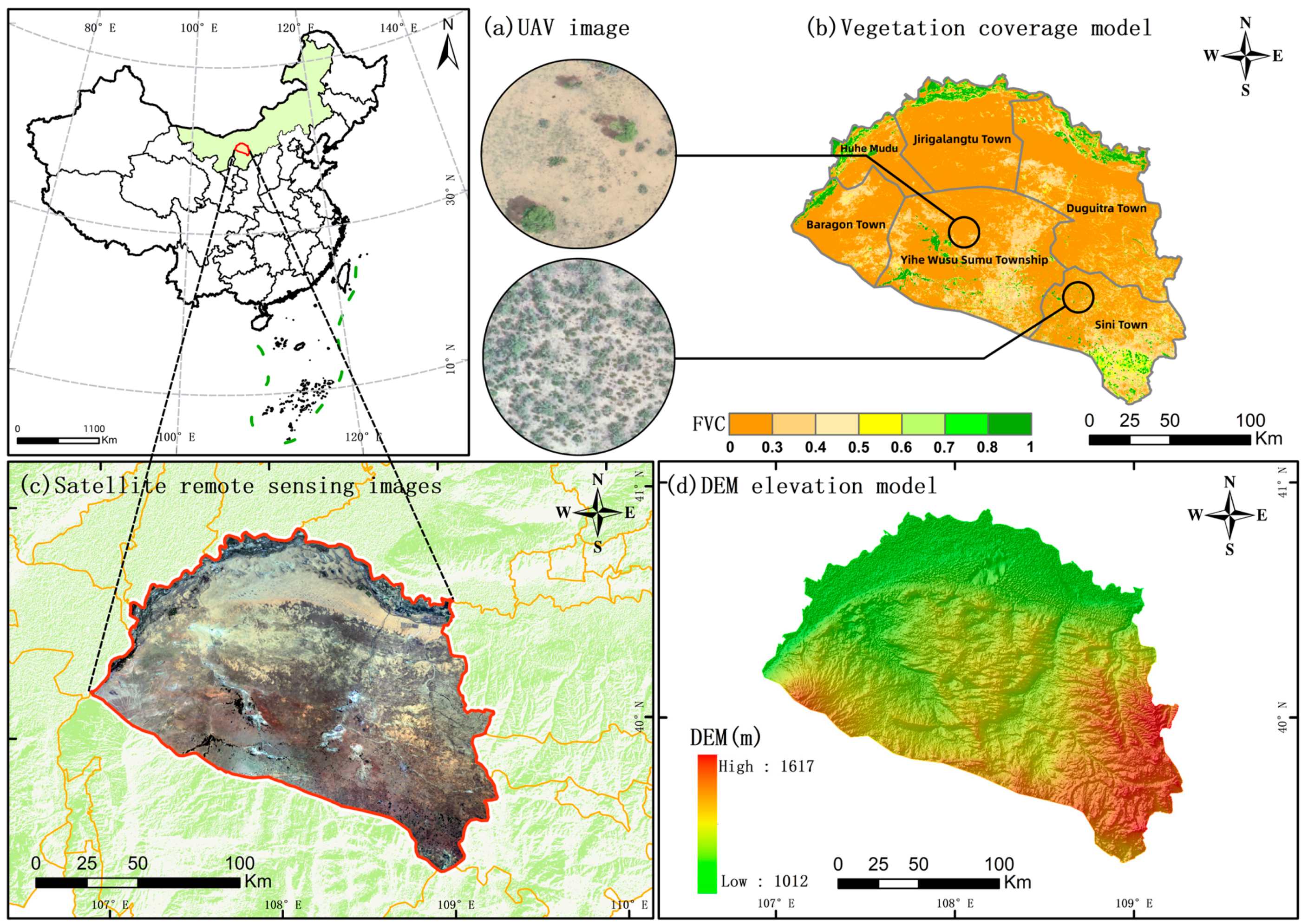
The study area is located in the Hangjin Banner, Ordos City, Inner Mongolia Autonomous Region, northern China. Its latitude lies between 107°7′E and 108°55′E, and its longitude is between 39°38′N and 40°27′N; this area is an important part of the Inner Mongolia grassland. The average altitude of the region is 1100 m, and the average annual temperature is 8.6 °C, which is a typical temperate continental climate. The region is subject to perennial wind–sand erosion and precipitation scarcity, leading to extensive land desertification [34]. Its high altitude and complex topography make most of the area unsuitable for manual field monitoring. Therefore, first, high-resolution satellite remote sensing images were used to perform large-scale monitoring of land changes, and vegetation information was extracted to construct a vegetation cover model, which helped to assess the health status of vegetation and the degree of desertification. The topography and geomorphology information was obtained using DEM elevation data to help analyze the characteristics of surface undulation, slope, and slope direction in desert areas. This is of great significance for setting UAV flight parameters and judging the desertification development trend. Finally, the UAV visible light image was used to extract data on the actual situation of the study area accurately. Figure 1 shows an overview of the geographic location of the study area and a model of the vegetation cover in Hangjin Banner.
2.2. Research Methodology
2.2.1. Color Space
In the classification of feature information, the commonly used color space models are the RGB color space model, the Lab color space model, and the HSV color space model. Among them, RGB images contain three color channels: R, G, and B. Due to the large correlation between these channels, it is difficult to quantitatively analyze the features, and misclassification problems easily occur [35]. Moreover, there are still many factors affecting the classification accuracy in the field of visible light remote sensing, such as the shading texture produced by tall trees covering low vegetation areas, dry shrubs with fewer stems and leaves, and meadows with lower reflectance in deserts [36]. All of these physical factors seriously interfere with the classification accuracy and cause misclassification problems, which in turn have an impact on the monitoring and evaluation of land desertification and trend judgment.
However, the Lab color space consists of brightness factor L and chromaticity factors a and b. Although it extends the range of color expression, only the a channel has the ability to detect green vegetation [37,38]. Additionally, in the middle and low vegetation coverage interval, because the a channel does not have bimodal characteristics during the channel fitting process, it is also impossible to determine the range of vegetation pixel thresholds in the a channel; thus, the Lab color space is more limited in extracting data regarding the monitored vegetation. Compared with the RGB color space and Lab color space, the HSV color space model consists of three elements: hue, saturation, and value [39]. These three elements are completely in line with human visual characteristics, with more relative independence in remote sensing image processing, and the H (hue) value between different color features varies greatly [40]. The HSV color space model is a hexagonal vertebrae model, and the range of values of the H element is usually expressed in terms of the angular range [41]. The hue (H) value covers a range from 0 to 360°; the value of S (saturation) is directly proportional to the color intensity and determines the vividness of the color, which covers a value range from 0 to 100%; and the V (value) indicates the brightness of the color; the larger the value, the higher the luminance, and it ranges from 0 to 100% [42]. Additionally, different color types can be represented by directly changing the H channel; saturation and brightness are also independent of each other, and adjusting the S and V values can arbitrarily change the vividness of the color without changing the color type [43]. This makes the vegetation index determined using the HSV color space have unique advantages in desert vegetation information extraction and more suitable for desert vegetation detection. Therefore, based on the above reasons, this paper proposes the HSVGVI to extract desert vegetation information for monitoring. In addition, the HSV color space model is shown in Figure 2.
2.2.2. Methodological Process
Although high-resolution satellite remote sensing images (Landsat-8) have the ability to monitor vegetation information on a large scale, they cannot detect desert vegetation with high precision [44]. UAV remote sensing has the advantage of high precision and is not affected by complex terrain, but the coverage of the monitoring area is limited, and the preprocessing and splicing of images take longer; thus, it is time-consuming [45,46]. For this reason, we used a combination of high-resolution satellite remote sensing images and UAV visible light images to extract vegetation information in the study area. First, high-resolution satellite remote sensing images were used to establish the vegetation coverage (FVC) model of the study area, and the area with lower vegetation coverage (FVC < 0.3) was set as the key monitoring area of land desertification. Visible light remote sensing images from UAVs were then utilized to accurately extract desert vegetation information.
Furthermore, in visible light image desert vegetation detection, the detection accuracy is mainly affected by the following two factors: dry wood vegetation containing low chlorophyll and vegetation under the cover of shadow texture. Therefore, we took the above two influencing factors as the main object of study, and based on these two influencing factors, we divided the new regional samples in the study area. The criteria for sample delineation were as follows: counting the number of pixels using the pixel-by-pixel method and calculating the area occupied by the two main influencing factors to ensure that the area of the influencing factors accounts for more than 20% of the total area of the samples (to prevent the influencing factors from being overlooked because they account for a smaller proportion), thus delineating the areas with dense vegetation and those with more shadows in the study area. With the above sample area, the extraction effect and extraction accuracy of the HSVGVI can be tested. Figure 3 shows a UAV visible remote sensing image, with (a) showing an area with dense vegetation and (b) showing an area with multiple shadows.
The detailed experimental procedure of this paper consisted of the following eight steps:
- (1)
- First, we carried out data collection and integration using three Landsat8 images near January 2021, all of which have less than 3% cloud cover, with a spatial resolution of 30 m, and path/row numbers of 129/32, 128/32, and 128/33, and then we used the red and near-infrared bands of Landsat8 images to compute the NDVI values and FVC values. After identifying the study area, we used a DJI Elf 4 rtk (multi-spectral version) drone to acquire a light remote sensing image of the study area. The UAV has the following wavelengths and spectral widths: blue (B): 450 nm ± 16 nm; green (G): 560 nm ± 16 nm; red (R): 650 nm ± 16 nm; red edge (RE): 730 nm ± 16 nm; and near-infrared (NIR): 840 nm ± 26 nm. It has a spatial resolution of 0.1 m, and the specific flight parameters for the study area were set as follows: default speed: 7.9 m/s; shooting mode: timed shooting; heading repetition; and line repetition rates of 65% and 45%.
- (2)
- Subsequently, the Lantsat8 high-resolution satellite remote sensing image was subjected to image preprocessing using ENVI 5.3.1 (64-bit) software’s Radiometric Calibration tool for each band in the data, with the interleaved output type selected as BLL and the output data type selected as Float to complete the radiometric calibration. The atmospheric correction was then performed using the FLAASH (fast line-of-sight atmospheric analysis of spectral hypercubes) method. After completing the atmospheric correction, the image was spliced with the Seamless Mosaic tool, and its background value was set to 0 (ignoring the background value). The sampling method was chosen as the Cubio convolution method for image stitching calculation.
- (3)
- The normalized vegetation index model (NDVI) was established, and the vegetation cover (FVC) of the study area was calculated based on the NDVI, in which the NDVI and FVC were determined using Equations (1) and (2).where is the near-infrared band, and is the red band.where and are the NDVI values for fully vegetated versus bare ground or unvegetated pixels, respectively [47]. The and values vary over time and space due to atmospheric and surface conditions, year, season, and region [48,49]. In this study, 5% and 95% cumulative percentages were used as confidence intervals to determine the valid and values for the study area, respectively.
- (4)
- The vegetation cover model was analyzed, locating areas of land desertification and obtaining visible remote sensing images from drones;
- (5)
- Constructing HSVGVI vegetation index model based on unmanned aerial vehicle visible light remote sensing images;
- (6)
- The supervised classification of each vegetation index model was completed using the support vector machine (SVM) method. The support vector machine (SVM) is a machine learning method proposed by Vapnik in the 1990s, which was developed based on the VC (Vapnik–Chervonenkis) dimension theory and the principle of structural risk minimization in statistical theory. The basic idea of a support vector machine is to classify the input sample points by finding an optimal hyperplane. The principle of selecting the optimal hyperplane is to be able to distinguish the input sample points correctly and maximize the geometric interval from the sample points to the optimal hyperplane to obtain a better classification result [50]. Through the learning and training of the support vector machine, the parameters of the optimal hyperplane can be found, so as to obtain an efficient and accurate classification model. The principle is shown in Figure 4.Compared with other methods, the SVM algorithm performs well when dealing with small sample datasets because it can improve the generalization ability of the model and reduce the risk of overfitting by maximizing the classification interval. The SVM algorithm can also effectively deal with nonlinearly divisible data by mapping the data into a high-dimensional space, and classification is performed by finding the optimal hyperplane. Moreover, the SVM algorithm is mainly affected by support vectors, so outliers have less influence on it [51].
- (7)
- The confusion matrix, overall accuracy, producer accuracy, user accuracy, and error analysis were constructed to jointly verify the accuracy of classification (according to Foody [52], the Kappa coefficient is not suitable for comparing the accuracy of thematic maps, so the Kappa coefficient indicator was not used). Confusion matrices (CMs) are used as common evaluation tools in classification problems to visualize the performance and error analysis of classification models. The correspondence between the results of the classification algorithm on the samples and the actual situation is shown in the form of a matrix. By analyzing the confusion matrix, the accuracy of the vegetation index model can be calculated to further assess the performance of the classification algorithm [53].
- (8)
- Finally, the experimental classification results are analyzed through an accuracy evaluation of the experiment, and land desertification in the Hangjin Banner is discussed.
The flowchart of the experiment is shown in Figure 5.
3. Experiment and Analysis
3.1. Determination of the Vegetation Index and Construction of Its Model
By constructing an RGB color space and determining the HSVGVIs, the corresponding vegetation index models were established in the study area. Through supervised classification and accuracy verification, the ability of each vegetation index to extract vegetation information was statistically analyzed, and the vegetation indices that still maintained high accuracy in extracting vegetation information in harsh desert environments were selected to explore the key factors affecting the extraction of vegetation information.
3.1.1. Vegetation Index Based on RGB Color Space
Vegetation indices based on the RGB color space are calculated by combining multiple bands according to the spectral characteristics of vegetation and are widely used to monitor the extraction of vegetation cover data and evaluate the growth of vegetation. In the field of UAV visible remote sensing, there are more than 150 vegetation indices [54], such as the EXG (excess green index) [55], RGBVI (red–green–blue vegetation index) [56], MGRVI (modified green–red vegetation index) [57], NGRDI (normalized green–red difference index) [58], and VDVI (visible-band difference vegetation index) [59]. These five vegetation indices are based on the reflective and absorptive properties of plants considering electromagnetic waves and utilize the component of RGB in visible light to accurately describe the information of various types of vegetation [60]. All of them are vegetation indices calculated based on the difference between green and red bands, which are highly sensitive to the changes in vegetation chlorophyll content [61]. Therefore, these vegetation indices were utilized as control tests. The accuracy was verified by constructing a confusion matrix model and calculating the overall accuracy, producer accuracy, and user accuracy, and finally, the differences between the HSVGVI vegetation indexes and those based on the RGB color space were comprehensively analyzed in terms of their ability to extract vegetation information. The specific construction formula is shown in Table 1:
3.1.2. Build HSVGVI
The UAV visible remote sensing image is an RGB color space image, so the RGB color space should be converted into an HSV color space first. The specific conversion relationship is shown in Equation (3):
where R, G, and B are the value domains of the R, G, and B channels, respectively. The meaning of Cmax is to take the maximum value in the brackets, and the meaning of Cmin is to take the minimum value in the brackets.
First, we normalized the R, G, and B color channels and selected the maximum and minimum values of R, G, and B [62]. Then, the hue, saturation, and value parameters were determined using Equation (4) to convert the RGB color space into the HSV color space as follows:
where H, S, and V values represent the specific values of hue, saturation, and brightness, respectively. The value of is obtained from Equation (1).
There is a difference in color distribution between RGB and HSV. In the RGB color space, the color dots are evenly distributed, while in the HSV color space, the color dots are more concentrated in the center area of the cone. Therefore, during the conversion process, some colors may be more densely distributed in HSV images and shift or create new color effects, giving a different appearance to the overall color of the HSV images. The difference in hue (H) between different categories of features in HSV images is large, so compared to RGB images, there is a higher degree of differentiation between different color types, which can be used to construct the HSVVI from HSV images.
In order to further expand the differentiation between different types of features, and to distinguish desert vegetation from other features such as bare soil, the brightness (V) and saturation (S) values of the image can be increased by 10–20% (in this paper, the value is taken to be 15%), which can maximize the color intensity and vividness of the image without changing the clear structure of the image [63]. Next, it is necessary to output the HSVVI again as an RGB image with channel enhancement. Although at this stage, the color information of the HSVVI is expressed through H, S, and V color channels, the final output form is still presented through RGB color channels. Therefore, after increasing the S and V values, saving the effects as RGB images directly can avoid the color shift again when converting the HSV color space to RGB color space. The specific method is shown in Equation (5).
where denotes the operation of taking the modulus (remainder) of 2.
The spectral reflectance of green vegetation in visible remote sensing images is characterized by the highest reflectance in the green band, which is greater than the reflectance in the red and blue bands. That is, vegetation absorbs red and blue light with higher intensity and absorbs green light with lower intensity. Lastly, using this feature, the HSVGVI was constructed by mixing the R channel with the G channel through channel mixing, after which the G channel was the enhanced channel, that is, the G value was enhanced to two times the original one. The specific construction method (6) is shown below.
where , , and are the values of the R, G, and B channels in the HSVVI model, respectively, and the HSVGVI model can be obtained through the calculation of channel enhancement.
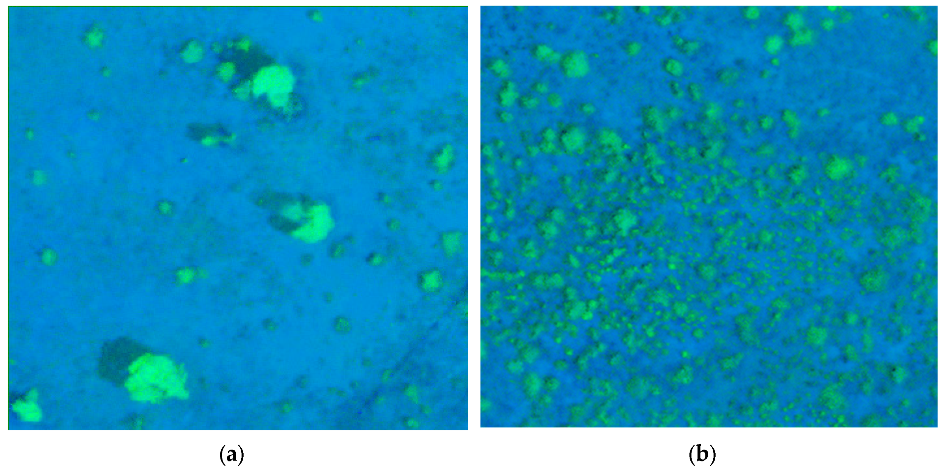
The HSVGVI can be used to monitor vegetation under shadow coverage, as well as dry shrub vegetation and meadows with fewer stems and leaves, and solve the problem of false classification caused by shadow texture coverage. Figure 6 shows an HSVGVI image for (a) a multi-shaded area and (b) a dense vegetation area.
4. Results
4.1. Building Index Models
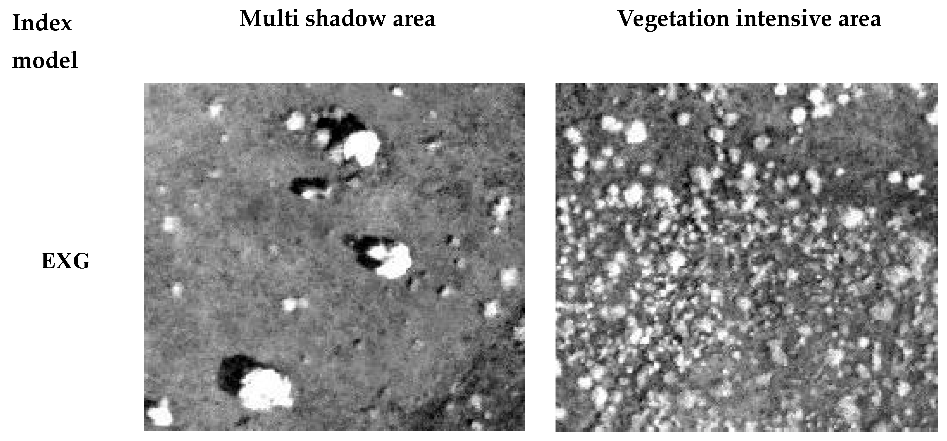
Based on the construction methods of various vegetation index models in the previous section, the EXG (excess green index), RGBVI (red–green–blue vegetation index), MGRVI (modified green–red vegetation index), NGRDI (normalized green–red difference index), and VDVI (visible-band difference vegetation index) models were constructed in the RGB color space through band combination calculation. The HSVVI (hue–saturation–value vegetation index) and HSVGVI (hue–saturation–value green enhancement vegetation index) models were constructed based on the HSV color space. All vegetation index models are shown in Figure 7.
4.2. Supervision Classification of Each Model
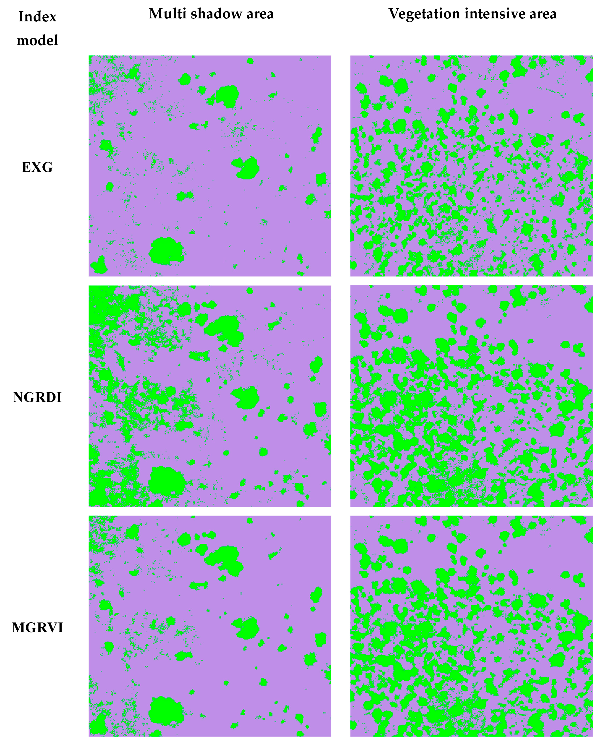
After constructing the vegetation index model, the supervised classification of different features was carried out based on a support vector machine (SVM), the aim of which was to divide the study samples into two categories (vegetation category and bare soil category) with maximum spacing and find the hyperplane that maximized the boundary between the two categories to achieve classification. By finding a set of support vectors as the closest training sample points to the hyperplane, these support vectors are used to determine the classification boundaries and make classification decisions [64]. To ensure the accuracy of supervised classification, the separation between the training samples of different regions of interest in the supervised classification samples was kept greater than 1.9. To ensure the accuracy of supervised classification, a computerized ROI separability tool was used to compute the separation between any classes when separating different ground objects. Separability was based on the Jeffries–Matusita distance and transition separability to measure the separability between different categories. Its range was [0, 2]. The greater the separation, the better the discriminatory ability, and a separation degree of greater than 1.8 was considered satisfactory whereas that greater than 1.9 was considered accurate [65]. Based on the spatial resolution of the UAV, the area of a single pixel was calculated. By means of field surveys, validation sample squares were established on a per-pixel basis. The feature attributes (vegetation or bare soil) that accounted for more than 50% of the features within the sample squares were recorded as attributes per pixel. Sample-by-sample vectorization was performed based on the percentage of each type of feature within each sample square. Finally, validation samples were obtained from the feature information in each pixel. Using this method, the validation samples of multi-shaded areas and vegetation-dense areas were obtained for subsequent accuracy validation. Figure 8 shows the supervised classification results of these seven vegetation indices compared with the validation samples (green color indicates vegetation and purple color indicates bare soil):
Based on the two different types of study areas, preliminary findings can be revealed by comparing and analyzing the supervised classification results in Figure 7 and the raw UAV image data: In the multi-shaded type region, due to the influence of high-intensity light, the branching and leafy tree canopy produces a deep shadow texture, which covers a considerable area of low shrub vegetation on the ground surface, and due to the large correlation of the three channels in the RGB color space, which is impossible to quantitatively analyze, a large number of misclassification problems occur, which seriously affect the accuracy of the vegetation extraction. The EXG, NGRDI, MGRVI, VDVI, and RGBVI cannot be used to extract low vegetation areas under shadow coverage, resulting in some vegetation pixels being misclassified as bare soil pixels. On the other hand, the HSVVI and HSVGVI models constructed based on the HSV color space, in which the color types in the image are only controlled using the H channel, are relatively independent and have a larger degree of differentiation; thus, they can better detect the vegetation under shadow coverage.
The densely vegetated areas are located in arid and semi-arid regions with mostly low and dry shrub vegetation, and the grass on the ground is too sparse and has low chlorophyll content. This results in poor green light reflectance and leads to the inability to recognize some of the vegetated areas. NGRDI, MGRVI, and HSVGVI models can maintain a certain accuracy in detecting vegetation in grassland areas because these three vegetation indices enhance the green channel during the model construction. All other vegetation indices have more serious misclassification problems, resulting in generally low accuracy in detecting vegetation cover in the study area.
4.3. Calculation and Statistics of the Percentage of Physical Characteristics of Each Place
In this paper, reference data such as the total area of the study samples, specific vegetation area, and non-vegetation area were obtained through field investigations, which were used to evaluate the accuracy of the feature coverage determined with each vegetation index model. The following calculation method was used for feature coverage: the ratio of the area of two types of features after supervised classification using each vegetation index model to the total area of the study area is taken as the coverage of these features in the study area, as shown in Equation (7):
where is the coverage of a feature, is the area of a feature, and is the total area of the study area.
Based on the above calculation process, the percentage of data for each feature and the vegetation cover of each vegetation index after supervised classification can be obtained. By comparing and analyzing them with the reference data, the ability of various vegetation indices to extract vegetation information and monitor the process of land desertification can be preliminarily judged. Vegetation coverage statistics for multi-shaded and densely vegetated areas are presented in Table 2.
4.4. Accuracy Evaluation and Error Analysis of Supervised Classification Results
4.4.1. Accuracy Assessment and Construction of Confusion Matrix
In this study, the entire sample area was first divided into a grid by individual pixels, and the area occupied by individual pixels was calculated based on the spatial resolution of UAV images. Then, a field survey was conducted to establish validation sample squares based on the area of each pixel. The feature attributes (vegetation or bare soil) with more than 50% of the area within a sample square were labeled as attributes for that sample square. Subsequently, the feature information of each sample square was vectorized, and the sample squares were vectorized into validation sample points, which were integrated and used to construct validation samples for supervised classification. Next, the UAV visible images were visually interpreted, and the interpretation results were compared with the validation sample in order to further modify and correct any unreasonable points in the validation sample. Finally, this validation sample was used to evaluate the accuracy of the supervised classification results. In addition, we constructed a confusion matrix. The overall accuracy, producer accuracy, and user accuracy were used as accuracy evaluation indicators, and the specific construction method is shown in Equations (8)–(10).
where P is the total number of samples, k is the total number of categories, is the number of correctly categorized samples, is the number of samples in category , and is the number of samples predicted to be in category .
4.4.2. Error Analysis
To further verify the accuracy of the supervised classification results, the following equation was utilized for error analysis:
where is the vegetation coverage rate after the supervised classification of each vegetation index, and is the vegetation coverage rate measured in the field. Due to the fact that was used as a precision evaluation control experiment for the supervised classification results of various vegetation indices, detailed field measurements were conducted by delineating the study area to ensure the accuracy of .
In summary, the results of accuracy evaluation, error analysis, and confusion matrix for the multi-shaded vegetation areas and densely vegetated areas are shown in Table 3, Table 4, Table 5 and Table 6, respectively. ‘Vegetation’ and ‘bare soil’ in Table 4 and Table 6 indicate the number of vegetation samples and bare soil samples, respectively.
4.5. Analysis of Supervised Classification Results
According to the supervised classification results, it can be seen that in the multi-shaded vegetation area, although the supervised classification accuracies of all vegetation indices are above 90%, a significant error occurs, which is mainly due to the following three factors: (1) a misclassification problem occurs in the multi-shaded area due to the coverage of the shaded texture; (2) a misclassification problem occurs in the densely vegetated area due to the presence of a large number of dry shrubs; and (3) the percentage of vegetation area in the region is much smaller than the percentage of bare soil area, leading to the overall supervised classification accuracy being falsely high.
Based on this, we verified the accuracy of vegetation detection by constructing confusion matrices, as well as the overall accuracy, producer accuracy, user accuracy, and error analysis models; in this case, the error analysis is based only on the percentage of vegetation obtained, so it is more intuitive to determine the vegetation cover. The high accuracy of producers and low accuracy of users indicate that although the visible vegetation index model can be used to roughly identify vegetation coverage, there is a very serious misclassification problem, and its accuracy makes it difficult to use this model for land desertification monitoring. In order to further explore whether the HSVGVI and other vegetation indices may misclassify as a result of shadow texture, dry shrub vegetation, etc., the study area was quantitatively divided again, the influence factors were amplified, and the percentage of the vegetation sample area was increased so as to ensure that the supervised classification results were intuitive and applicable to the evaluation of accuracy.
4.6. Comparison between Vegetation Samples under Shadow Coverage and Dry Shrub Vegetation Samples
In order to further validate the misclassification problem described in the previous section, the vegetation samples under shadow coverage and dry shrub vegetation samples were divided in the study area. The specific division principles were as follows: (1) Since the number of vegetation images in the original sample accounted for a small percentage and the number of non-vegetation images accounted for a large percentage, even if the problem of misclassification of vegetation images occurred, the impact on the final accuracy evaluation results would be small, resulting in the accuracy presenting a false high. Therefore, increasing the percentage of vegetation area can better and more realistically reflect the accuracy problem due to misclassification and can also ensure the intuitiveness and authoritativeness of supervised classification accuracy. (2) The vegetation samples under shadow coverage were divided, and the shadow-texture-influencing factors were amplified. (3) The vegetation samples of low shrubs with fewer stems and leaves were divided, and the influencing factors for dry shrubs were amplified. By using the above division principles, the samples were obtained after amplifying the influencing factors, which could better show the advantages of the HSVGVI in shadow elimination and vegetation detection. Figure 9a shows the vegetation samples under shadow coverage, and Figure 9b shows the dry shrub vegetation samples.
4.7. Proportion and Accuracy Verification of Objects in Different Regions
By analyzing the supervised classification results of vegetation samples under shadow coverage and dry shrub vegetation samples, the proportion of objects in each region with these two samples was obtained. Table 7 shows the vegetation coverage statistics for the shaded coverage and dry shrub areas.
Based on the supervised classification results and actual field measurement data, we constructed a confusion matrix and calculated the overall classification accuracy, producer accuracy, and user accuracy. The specific accuracy evaluation is shown in Table 8, Table 9, Table 10 and Table 11. Table 8 is the accuracy evaluation results of vegetation samples under shadow coverage, and Table 9 is its confusion matrix. Table 10 is the accuracy evaluation results of vegetation samples of dry shrubs, and Table 11 is its confusion matrix. ‘Vegetation’ and ‘bare soil’ in Table 9 and Table 11 indicate the number of vegetation samples and bare soil samples, respectively.
According to Table 8 and Table 10, by increasing the percentage of vegetation area, the supervised classification accuracy of each vegetation index model is no longer falsely high due to fluctuations in the values and is more intuitive and authoritative. However, there is still a large error, which reflects that the presence of shaded texture and low shrubs containing fewer green leaves have a greater impact on the accuracy of vegetation detection.
In the vegetation samples from areas under shaded coverage, the vegetation indices constructed based on the RGB color space are greatly affected by the shadow texture, and their overall accuracies are generally low: The detection errors of vegetation coverage are all greater than 40%. Among the different vegetation indices, although the total accuracy of the NGRDI can reach 84.29%, and the producer accuracy can reach 84.58%, its user accuracy is only 82.63%, indicating that there are many misclassification problems. In addition, the producer accuracy of other RGB-space vegetation indices is generally low, but the user accuracy can reach more than 90%, which indicates that there are many misclassification problems in the classification process. This is due to the masking of shadow texture, and many vegetation pixels are “lost” in the classification. These RGB spatial vegetation indices can only extract the more obvious vegetation pixels, but it is difficult to extract the vegetation pixels covered by shadow textures. On the other hand, the supervised classification accuracy of the HSVGVI is as high as 97.78%, its vegetation cover detection error is only 8.21%, the producer’s accuracy coefficient is 89.58%, and the user’s accuracy is 99.61%. This indicates that it has a better extraction and classification accuracy, and compared with the RGB-space vegetation indices, the HSVGVI can eliminate the effect of shaded textures, which makes it more suitable for the detection of desert vegetation.
In the dry shrub vegetation samples, the overall accuracy of vegetation indices in RGB color space is lower than 85%, generally around 70%, and the extraction error of vegetation cover is more than 25%; the producer accuracy fluctuates between 37% and 72%, and the user accuracy is above 90%. Since the VDVI is more sensitive to the green wave band, its classification accuracy can reach 83.88% with an error of 25.44%; the producer accuracy is 71.61%, and the user accuracy is 96.05%. The phenomenon that the producer accuracy is lower, whereas the user accuracy is higher in the RGB vegetation indices also indicates that the vegetation containing fewer stems and leaves is difficult to detect, which leads to a serious misclassification problem. However, the HSVGVI has the advantages of the quantitative analysis of relatively independent hues in the HSV color space as well as green channel enhancement, so the overall accuracy, producer accuracy, and user accuracy can be up to 94.45%, 89.58%, and 99.61%, respectively. The error analysis is only 10.00%, which indicates that this index is suitable for classifying low shrubs with fewer green leaves and solves the problem of misclassification observed with vegetation indices in the RGB color space.
In conclusion, the HSVGVI not only inherits the unique advantages of the HSV color space but also has the ability to enhance the green channel and greatly reduce the influence of dark shadow texture, which enables us to extract the low shrub vegetation data with fewer green leaves more clearly, and the overall accuracy, producer’s accuracy, and user’s accuracy can be achieved at a high level.
5. Discussion
5.1. Comparative Analysis of Various Samples in the Research Area
In this study, the proportion of vegetation and non-vegetation, the classification accuracy, and the producer accuracy in the two groups of study areas were determined separately. By comparing and analyzing the above data, the following conclusions are drawn: By establishing the second group of research areas, the two influencing factors of shadow texture and dry shrub vegetation were further amplified. By observing the trends of the overall accuracy, producer accuracy, and user accuracy of the vegetation indices constructed based on the RGB color space, it was found that the overall accuracy and producer accuracy coefficients decreased significantly, and the error gradually increased, but the user accuracy still remained at a certain level. This indicates that these vegetation indices can extract some more “obvious” (not affected by influencing factors) vegetation samples in the image, but there is a significant misclassification problem, as both shadow-covered vegetation pixels and dry vegetation pixels are misclassified as bare soil pixels, resulting in lower overall accuracy and producer accuracy. On the other hand, the overall accuracy of the HSVGVI remains above 95%, the error rate is not more than 10%, and the user accuracy and producer accuracy are above 89%. In summary, the results show that the HSVGVI has the ability of shadow elimination and high-precision vegetation detection and thus is a better solution to the two major problems faced in desert vegetation detection.
5.2. Analysis of Land Desertification in Hangjin Banner
Through the vegetation cover model, it can be inferred that the land desertification problem in the Hangjin Banner is more serious, dominated by areas of medium and severe land desertification. For monitoring land desertification in the Hangjin Banner, we took a multi-shaded vegetation area and a densely vegetated area as examples, and the vegetation coverage of these two samples determined using the HSVGVI was 0.18 (extremely desertified area) and 0.39 (moderately desertified area). In the FVC model of high-definition satellite remote sensing images, the vegetation coverage of these two samples was determined by inputting the geographic coordinates, and the vegetation coverage of these two samples was 0.3 (severely desertified area). High-resolution satellite remote sensing images could only roughly estimate the vegetation cover, and their accuracy was not sufficient to accurately classify land desertification in the sample area. Therefore, we monitored land desertification by combining multi-source remote sensing images, using high-resolution satellite images to initially locate the areas with land desertification problems, and then extracted the vegetation information in the area by using UAV visible remote sensing images and the HSVGVI, so as to determine the grading of the degree of land desertification with high precision and provide data and technical support for the monitoring and prevention of land desertification in the Hangjin Banner.
6. Conclusions
The purpose of this paper is to combine high-resolution satellite remote sensing images and UAV visible images to evaluate the land desertification status of the Hangjin Banner, Bayannur City, Northwest China, as the study area. First, high-resolution remote sensing images were used to establish a vegetation coverage model to locate land desertification areas (FVC < 0.3). Then, UAV visible light images were used to extract desert vegetation information, which made the evaluation of land desertification more efficient and precise, with cheaper labor and less time-intensiveness.
Due to the strong light in the desert, the resulting shadow texture is deeper, and the shading of the low vegetation areas as a result of the shadow texture seriously affects the accuracy of vegetation extraction. In addition, due to climatic reasons, deserts are mostly dry shrubs with fewer stems and leaves, which also leads to the serious misclassification of vegetation indices in the RGB color space. For this reason, this paper proposes a new vegetation index, the HSVGVI, which is based on the HSV color space and is determined by using the channel enhancement method, which can eliminate the shadow texture to a greater extent. At the same time, it inherits the unique advantages of the HSV color space (the relative independence of the H channel), so it has a high sensitivity to the classification of green vegetation. Compared with the vegetation index models constructed based on the RGB color space, the HSVGVI shows higher accuracy and better adaptability in desert vegetation detection. The accuracy of the HSVGVI was verified by constructing a confusion matrix; calculating the overall accuracy, producer accuracy, and user accuracy; performing an error analysis; and using the vegetation index in the RGB color space as a control experiment. In order to further validate the advantages of the HSVGVI over the traditional vegetation index, this study focused on the difficult factors in the new research samples (vegetation samples under shadow coverage and dry shrub vegetation samples) through quantitative analysis and research methods. It was found that the overall accuracy of the vegetation index classifications based on the RGB color space was generally lower than 80%, the producer accuracy was generally lower than 70%, and the error was generally greater than 25%. By contrast, the classification accuracy of the HSVGVI could reach more than 95%, the producer accuracy was more than 89%, the user accuracy could reach more than 95%, and the error analysis was controlled below 10%. Thus, the influence of shadow texture is eliminated and the problem of misclassification of bare soil is solved.
In summary, the HSVGVI has the advantage of the HSV color space, allowing us to control the color in the image only through the H channel. At the same time, the HSVGVI has a high sensitivity in terms of recognizing green vegetation and can accurately recognize the green elements in the vegetation of dry shrubs. Therefore, the HSVGVI can provide high-precision vegetation information for land desertification assessment through UAV visible remote sensing images, and the HSVGVI model is more convenient to construct and has higher classification accuracy than the vegetation index models constructed based on the RGB color space.
Author Contributions
Conceptualization, Y.L.; data curation, Z.D., D.S. and W.S.; methodology, Y.L. and Z.S.; project administration, Y.L.; supervision, Y.L. and Y.J.; writing—original draft preparation, Z.S.; writing—review and editing, Y.L. and Y.J. All authors have read and agreed to the published version of the manuscript.
Funding
This research was funded by the Major Project of High-Resolution Earth Observation System of China (No. GFZX0404130304); the Open Fund of Hunan Provincial Key Laboratory of Geo-Information Engineering in Surveying, Mapping and Remote Sensing, Hunan University of Science and Technology (No. E22201); a grant from State Key Laboratory of Resources and Environmental Information System(NO); and the Innovation Capability Improvement Project of Scientific and Technological Small and Medium-sized Enterprises in Shandong Province of China (No. 2021TSGC1056).
Data Availability Statement
Restrictions apply to the availability of these data. Data were obtained from third parties and are available from the authors after obtaining permission from them. These third parties are noted in the Acknowledgments.
Acknowledgments
The authors thank the administrative division data provider used in this article; Resource and Environmental Science Data Center of Chinese Academy of Sciences (https://www.resdc.cn/, accessed on 27 September 2023). Additionally, the authors would like to thank Hangjin Banner DEM elevation data provider; Geospatial Data Cloud (https://www.gscloud.cn/, accessed on 29 September 2023).
Conflicts of Interest
Weiwei Sun was employed by Shandong Zhengyuan Digital City Construction Co., Ltd. The remaining authors declare that the research was conducted in the absence of any commercial or financial relationships that could be construed as a potential conflict of interest. The funders had no role in the design of the study; in the collection, analyses, or interpretation of data; in the writing of the manuscript; or in the decision to publish the results.
References
- Shao, W.Y.; Wang, Z.Q.; Guan, Q.Y. Environmental sensitivity assessment of land desertification in the Hexi Corridor. Catena 2023, 220, 106728. [Google Scholar] [CrossRef]
- Hu, Y.; Han, Y.; Zhang, Y. Land desertification and its influencing factors in Kazakhstan. J. Arid. Environ. 2020, 180, 104203. [Google Scholar] [CrossRef]
- Wang, W.L.; Jiang, Y.M.; Wang, G.; Fang, M. Multi-Scale LBP Texture Feature Learning Network for Remote Sensing Interpretation of Land Desertification. Remote Sens. 2022, 14, 3486. [Google Scholar] [CrossRef]
- Ding, X. A Study on the Dynamic Changes of Land Desertification in Inner Mongolia Autonomous Region. Master’s Thesis, Northeast Agricultural University, Harbin, China, 2018. [Google Scholar]
- Wang, Y.F.; Kang, Y.; Ma, H.W. Assessment of Land Desertification and Its Drivers on the Mongolian Plateau Using Intensity Analysis and the Geographical Detector Technique. Remote Sens. 2022, 14, 6365. [Google Scholar] [CrossRef]
- Ye, R.H. The Current Situation and Prevention Measures of Land Desertification in Inner Mongolia. West. Resour. 2008, 27, 37–39. [Google Scholar]
- Han, J.Z. Research on Vegetation Recognition Method of UAV Images Based on Deep Learning. Master’s Thesis, Beijing Forestry University, Beijing, China, 2018. [Google Scholar]
- Li, Y.; Yu, H.Y.; Wang, Y. Urban vegetation classification based on UAV reconstructed point clouds and images. Remote Sens. Land Resour. 2019, 31, 1–7. [Google Scholar]
- Yang, H.Y. Study on Species Classification of Desert Grasslands Based on Unmanned Aerial Vehicle Hyperspectral Remote Sensing. Ph.D. Thesis, Inner Mongolia Agricultural University, Hohhot, China, 2019. [Google Scholar]
- Hamylton, S.M.; Morris, R.H. Evaluating techniques for mapping islandvegetation from unmanned aerial vehicle (UAV) images: Pixel classification, visual interpretation andmachine learning approaches. Int. J. Appl. Earth Obs. Geoinf. 2020, 89, 1–14. [Google Scholar]
- Prabha, A.R.; Anita, S.M. Classification of shoreline vegetation in the Western Basin of Lake Erie using airborne hyperspectral imager HSI2, Pleiades and UAV data. Int. J. Remote Sens. 2019, 40, 3008–3028. [Google Scholar] [CrossRef]
- Xu, D.W. Changes in Distribution and Analysis of Different Grassland Types in Hulunbeier Grassland Area. Ph.D. Thesis, Chinese Academy of Agricultural Sciences, Beijing, China, 2019. [Google Scholar]
- Wang, M.; Zhang, X.C. Combining object-oriented forest resource classification with random forest. J. Surv. Mapp. 2020, 49, 235–244. [Google Scholar]
- Liu, B. Research on Crop Classification Based on UAV Remote Sensing Images. Master’s Thesis, Chinese Academy of Agricultural Sciences, Beijing, China, 2019. [Google Scholar]
- Bryson, M.; Reid, A.; Ramos, F. Airbome vision based mapping and classification of largefarmland environments. J. Field Robot. 2010, 27, 632–655. [Google Scholar] [CrossRef]
- Feng, Y.Y.; Wang, S.H.; Zhao, M.S. Monitoring of Land Desertification Changes in Urat Front Banner from 2010 to 2020 Based on Remote Sensing Data. Water 2022, 14, 1777. [Google Scholar] [CrossRef]
- Hong, X.L.; Zhang, Y.T.; Wang, T.C. Research on development countermeasures for the application of drone remote sensing technology in agriculture. Northeast. Agric. Sci. 2023, 48, 140–144. [Google Scholar]
- Hong, Z.X. Research Advance in Remote Sensing to Land Desertification Monitoring. Adv. Mater. Res. 2013, 864–867, 2817–2820. [Google Scholar] [CrossRef]
- Li, A.; Wei, X.; Li, Z.X. Precision analysis of high-resolution image land use interpretation in soil erosion dynamic monitoring. Sci. Soil Water Conserv. China 2018, 16, 8–17. [Google Scholar]
- Zhang, H. High-resolution satellite imagery for monitoring desertification: A case study in an arid region of China. J. Arid. Land 2019, 11, 508–521. [Google Scholar]
- Chen, X.; Liu, G. Satellite-based high-resolution mapping of desertification dynamics using texture analysis. Remote Sens. 2018, 10, 477. [Google Scholar] [CrossRef]
- Sun, J.X.; Zhong, C.; He, H.W. Continuous remote sensing monitoring of land desertification and its changes in China from 2000 to 2015. J. Northeast. For. Univ. 2021, 49, 87–92. [Google Scholar]
- Yang, Q.; Ye, H.; Huang, K.; Cha, Y.Y. Using drone images to construct crop surface models for estimating sugarcane LAI. Trans. Chin. Soc. Agric. Eng. 2017, 15, 33. [Google Scholar]
- Li, W.; Hu, Y.; Chen, S.; Shen, H. Unmanned Aerial Vehicle Remote Sensing for Vegetation Extraction: A Review. Remote Sens. 2020, 12, 687. [Google Scholar]
- Wang, X.Q.; Wang, M.M.; Wang, S.Q. Vegetation information extraction based on visible light band unmanned aerial vehicle remote sensing. J. Agric. Eng. 2015, 31, 152–159. [Google Scholar]
- Li, D.S.; Liu, H.H.; Zhang, B.L. Green vegetation extraction method based on drone images. J. Kunming Metall. Coll. 2019, 35, 58–65. [Google Scholar]
- Bareth, G.H.; Bolten, A. Comparison of uncalibrated RGBVI with spectrometer-based NDVI derived from UAV sensing systems on field scale. Int. Arch. Photogramm. Remote Sens. Spat. Inf. Sci. 2016, 23, 837–843. [Google Scholar] [CrossRef]
- Ma, M.H.; Kong, L.S. Study on the Bioecological Characteristics of Pipa Chai on the Edge of the Hutubi Oasis in Xinjiang. J. Plant Ecol. 1998, 22, 237. [Google Scholar]
- Zhang, X.; Feng, Q.; Yang, F.; Li, Q. Unmanned aerial vehicle remote sensing for precision agriculture: A review. J. Sens. 2019, 11, 1–14. [Google Scholar]
- Wang, M.Q.; Yang, J.Y.; Sun, Y.K. Rapid extraction technology of vegetation coverage in abandoned mines using unmanned aerial vehicle remote sensing. Sci. Soil Water Conserv. China 2020, 18, 130–139. [Google Scholar]
- Zhu, J. Assessing the Feasibility of Using Low-cost Unmanned Aerial Vehicles for Forest Inventory–A Case Study on Variable Plot Sizes. Scand. J. For. Res. 2016, 31, 633–641. [Google Scholar]
- Wu, B.; Xu, R.; Xing, K.; Wang, L. A Novel Active Learning Framework for Crop Classification Using UAV Hyperspectral Data. Remote Sens. 2019, 11, 228. [Google Scholar]
- Yang, L.; Zhang, C.; Guo, H. Improved Classification of Unmanned Aerial Vehicle (UAV) Images with Convolutional Neural Networks. Remote Sens. 2018, 10, 1443. [Google Scholar]
- Yang, H.Y.; Du, J.M.; Ruan, P.Y.; Zhu, X.B.; Liu, H.; Wang, Y. Vegetation Classification of Desert Steppe Based on Unmanned Aerial Vehicle Remote Sensing and Random Forest. Trans. Optik 2021, 52, 186–194. [Google Scholar]
- Cai, C.D.; Huo, G.Y.; Zhou, Y.; Han, H. Underwater Image Restoration Based on Scene Depth Estimation and White Balance. Laser Optoelectron. Prog. 2019, 12, 031008. [Google Scholar]
- He, M.Y.; Cheng, Y.L.; Qiu, L.B. An algorithm of building extraction in urban area based on improved top-hat transformations and LBP elevation texture. Acta Geod. Cartogr. Sin. 2017, 20, 1116. [Google Scholar]
- Liu, J.F.; Li, D.B. Adaptive K-means image segmentation method based on Lab color space. Mech. Des. Manuf. Eng. 2018, 47, 23–27. [Google Scholar] [CrossRef]
- Niu, X.Y.; Zhang, L.Y.; Xie, W.T. Research on Cotton Coverage Extraction Method Based on Lab Color Space. J. Agric. Mach. 2018, 49, 240–249. [Google Scholar]
- Xing, J.; Zhang, Y.C.; Gao, J.C. Research on Improved Infrared and Visible Image Fusion Algorithm Based on HSV Color Space. Mech. Electron. 2022, 40, 15–19. [Google Scholar]
- Jia, F.L.; Tian, J.P.; Zhi, M.X. A landmark visual saliency model for virtual geographic experiments. J. Surv. Mapp. 2018, 47, 1114–1122. [Google Scholar]
- Shi, M.H.; Shen, L.; Long, S.Z. Correction of Color Space Conversion Formula from RGB to HSV. J. Basic Sci. Text. Univ. 2008, 81, 351–356. [Google Scholar]
- Sun, H.L.; Zhao, B.R.; Yu, W.X. Rapid Cloud Detection in Remote Sensing Images Based on HSV Color Space. Geospat. Inf. 2020, 18, 35–40+46. [Google Scholar]
- Guo, Y.H. Image segmentation based on HSV color space. Heilongjiang Metall. 2011, 31, 35–37. [Google Scholar]
- Dong, T.; Liu, J.; Qian, B. Estimating crop biomass using leaf area index derived from Landsat 8 and Sentinel-2 data. ISPRS J. Photogramm. Remote Sens. 2020, 168, 236–250. [Google Scholar] [CrossRef]
- Wang, Z.M. A Theoretical Review of Vegetation Extraction Methods Based on UAV. IOP Conf. Ser. Earth Environ. Sci. 2020, 546, 032019. [Google Scholar] [CrossRef]
- Na, S.-I.; Park, C.; So, K.; Ahn, H.; Kim, K.-D.; Lee, K. Estimation for Red Pepper Growth by Vegetation Indices Based on Unmanned Aerial Vehicle. Korean J. Soil Sci. Fertil. 2018, 51, 471–481. [Google Scholar] [CrossRef]
- Bai, S. Analysis of spatial and temporal changes of vegetation cover in Tumxuk City from 1993 to 2019. Shaanxi Water Resour. 2021, 6, 108–110+117. [Google Scholar]
- Zhang, L.; He, X.X. Dynamic changes of vegetation cover in the Huaihe River Basin based on NDVI. Yangtze River Basin Resour. Environ. 2012, 21 (Suppl. S1), 51–56. [Google Scholar]
- Yang, X.Q.; Zhu, W.Q. Vegetation cover estimation based on a modified subimage element model. J. Appl. Ecol. 2008, 8–12. [Google Scholar]
- Zhang, Y. Application of Machine Learning Method in Landslide Disaster Susceptibility Zoning. Master’s Thesis, Donghua University of Science and Technology, Shanghai, China, 2021. [Google Scholar]
- Lin, R.F. Landslide Susceptibility Assessment Based on Optimized Support Vector Machine Model. Master’s Thesis, Liaoning University of Engineering and Technology, Anshan, China, 2021. [Google Scholar]
- Foody, M.G. Explaining the unsuitability of the kappa coefficient in the assessment and comparison of the accuracy of thematic maps obtained by image classification. Remote Sens. Environ. 2020, 239, 111630. [Google Scholar] [CrossRef]
- Xu, L.L.; Chi, D.X. Machine Learning Classification Strategy for Unbalanced Datasets. Comput. Eng. Appl. 2020, 56, 12–27. [Google Scholar]
- Pinto, M.F.; Melo, A.G.; Honorio, L.M.; Marcato, A.L.M.; Conceicao, A.G.S.; Timotheo, A.O. Deep Learning Applied to Vegeta-tion Identification and Removal Using Multi dimensional Aerial Data. Sensors 2020, 20, 6187. [Google Scholar] [CrossRef] [PubMed]
- Gitelson, A.; Kaufman, Y.J.; Stark, R. Novel algorithms for remote estimation of vegetation fraction. Remote Sens. Environ. 2002, 80, 76–87. [Google Scholar] [CrossRef]
- Zhang, X.L.; Zhang, F.; Qi, Y.X.; Deng, L.F.; Wang, X.L.; Yang, S.T. New research methods for vegetation information extraction based on visible light remote sensing images from an unmanned aerial vehicle (UAV). Int. J. Appl. Earth Obs. Geoinf. 2019, 78, 215–226. [Google Scholar] [CrossRef]
- Bendig, J.; Yu, K.; Aasen, H.; Bolten, A.; Bennertz, S.; Broscheit, J.; Gnyp, M.L.; Bareth, G. Combining uav -based plant height from crop surface models, visible, and near infrared vegetation indices for biomass monitoring in barley. Int. J. Appl. Earth Obs. Geoinf. 2015, 39, 79–87. [Google Scholar] [CrossRef]
- Woebbecke, D.M.; Meyer, G.E.; Von, B.K. Color indices for weed identification under various soil, residue, and lighting condi-tions. Trans. ASAE 1995, 38, 259–269. [Google Scholar] [CrossRef]
- Qiao, L.; Tang, W.J.; Gao, D.H.; Zhao, R.M.; An, L.L.; Li, M.Z.; Sun, H.; Song, D. UAV-based chlorophyll content estimation by evaluating vegetation index responses under different crop coverages. Comput. Electron. Agric. 2022, 196, 106775. [Google Scholar] [CrossRef]
- Xie, B.; Yang, W.N. A new estimation method for fractional vegetation cover based on UAV visual light spectrum. Sci. Surv. Mapp. 2020, 45, 72–77. [Google Scholar]
- Lu, Y.F.; Song, Z.Q.; Li, Y.Q. A Novel Desert Vegetation Extraction and Shadow Separation Method Based on Visible Light Images from Unmanned Aerial Vehicles. Sustainability 2023, 15, 2954. [Google Scholar] [CrossRef]
- Tang, G.Y. Implementation of Conversion between RGB Color Model and HSV Color Model in VB. Technol. Inf. 2009, 2, 125–126. [Google Scholar]
- Wang, Z.M.; Zhang, L.; Bao, H. Adaptive Background Model Based on Hybrid Structure Neural Network. J. Electron. Sci. 2011, 39, 1053. [Google Scholar]
- Zhang, Z.L.; Feng, Y.B.; Zhao, Z.K. A SVM based oversampling method for imbalanced datasets. J. Comput. Eng. Appl. 2020, 56, 220–228. [Google Scholar]
- Wang, Z.C. Research on Classification Algorithm and Application of Remote Sensing Image Optimal Object Construction Based on Jeffries Matusita Distance; University of Chinese Academy of Sciences (Yantai Institute of Coastal Zone, Chinese Academy of Sciences): Yantai, China, 2022; p. 000017. [Google Scholar]
Figure 1.
Multi-source imagery data of the study area.

Figure 2.
HSV color space hexagonal vertebrae model.

Figure 3.
Study sample: (a) vegetation-intensive area; (b) multi-shaded vegetation area.

Figure 4.
Schematic diagram of SVM.

Figure 5.
Experimental flowchart.

Figure 6.
HSVGVI image: (a) multi-shaded area; (b) densely vegetated area.

Figure 7.
Modeling of each vegetation index for multi-shaded and densely vegetated regions.


Figure 8.
Supervised classification results for each vegetation index in multi-shaded and densely vegetated areas.
Figure 8.
Supervised classification results for each vegetation index in multi-shaded and densely vegetated areas.


Figure 9.
(a) Vegetation samples under shadow coverage; (b) supervised classification of vegetation samples from dry shrubs.
Figure 9.
(a) Vegetation samples under shadow coverage; (b) supervised classification of vegetation samples from dry shrubs.


Table 1.
Construction formula of vegetation indices based on RGB color space.
| Vegetation Index | Formula | Value Range |
|---|---|---|
| EXG (excess green index) | [–1, 2] | |
| RGBVI (red–green–blue vegetation index) | [–1, 1] | |
| MGRVI (modified green–red vegetation index) | [–1, 1] | |
| NGRDI (normalized green–red difference index) | [–1, 1] | |
| VDVI (visible-band difference vegetation index) | [0, 1] |
Table 2.
Statistics on percentage of vegetation in multi-shaded and densely vegetated areas.
| Index | Percentage of Vegetation in Multi-Shaded Areas | Percentage of Vegetation in Densely Vegetated Areas |
|---|---|---|
| EXG | 7.53% | 19.59% |
| VDVI | 7.67% | 35.01% |
| RGBVI | 8.83% | 25.18% |
| MGRVI | 8.66% | 30.08% |
| NGRDI | 22.19% | 34.53% |
| HSVVI | 10.08% | 29.05% |
| HSVGVI | 17.57% | 38.79% |
| Reference data from field measurements | 17.01% | 38.87% |
Table 3.
Accuracy assessment results for samples in multi-shaded areas.
| Vegetation Index | Overall Accuracy | Producer Accuracy | User Accuracy | Error Analysis |
|---|---|---|---|---|
| EXG | 89.63% | 41.67% | 94.08% | 55.73% |
| VDVI | 90.49% | 44.60% | 98.92% | 54.91% |
| RGBVI | 91.82% | 51.89% | 100.00% | 48.09% |
| MGRVI | 91.63% | 50.85% | 99.88% | 49.09% |
| NGRDI | 91.31% | 89.69% | 68.75% | 30.45% |
| HSVVI | 93.08% | 59.29% | 100.00% | 40.74% |
| HSVGVI | 99.13% | 99.10% | 95.95% | 3.29% |
Table 4.
Confusion matrix for multi-shaded region samples.
| Vegetation Index | Feature Type | Vegetation | Bare Soil |
|---|---|---|---|
| EXG | Vegetation | 8200 | 516 |
| Bare soil | 11,479 | 95,505 | |
| VDVI | Vegetation | 8776 | 96 |
| Bare soil | 10,903 | 95,925 | |
| RGBVI | Vegetation | 10,212 | 0 |
| Bare soil | 9467 | 96,021 | |
| MGRVI | Vegetation | 10,006 | 12 |
| Bare soil | 9673 | 96,009 | |
| NGRDI | Vegetation | 17,651 | 8022 |
| Bare soil | 2028 | 87,999 | |
| HSVVI | Vegetation | 11,668 | 0 |
| Bare soil | 8011 | 96,021 | |
| HSVGVI | Vegetation | 19,502 | 824 |
| Bare soil | 117 | 95,197 |
Table 5.
Results of accuracy evaluation of samples from densely vegetated areas.
| Vegetation Index | Overall Accuracy | Producer Accuracy | User Accuracy | Error Analysis |
|---|---|---|---|---|
| EXG | 76.27% | 44.66% | 88.56% | 49.56% |
| VDVI | 89.17% | 81.14% | 90.01% | 9.86% |
| RGBVI | 82.63% | 60.05% | 92.62% | 35.17% |
| MGRVI | 82.20% | 65.82% | 84.96% | 22.55% |
| NGRDI | 81.85% | 71.09% | 79.97% | 11.10% |
| HSVVI | 87.89% | 71.81% | 96.01% | 25.21% |
| HSVGVI | 95.73% | 89.43% | 99.52% | 0.13% |
Table 6.
Confusion matrix for samples from densely vegetated areas.
| Vegetation Index | Feature Type | Vegetation | Bare Soil |
|---|---|---|---|
| EXG | Vegetation | 20,070 | 2592 |
| Bare soil | 24,869 | 68,169 | |
| VDVI | Vegetation | 36,462 | 4049 |
| Bare soil | 8477 | 66,712 | |
| RGBVI | Vegetation | 26,988 | 2151 |
| Bare soil | 17,951 | 68,610 | |
| MGRVI | Vegetation | 29,578 | 5236 |
| Bare soil | 15,361 | 65,525 | |
| NGRDI | Vegetation | 31,947 | 8002 |
| Bare soil | 12,992 | 62,759 | |
| HSVVI | Vegetation | 32,271 | 1341 |
| Bare soil | 12,668 | 69,420 | |
| HSVGVI | Vegetation | 40,187 | 192 |
| Bare soil | 4752 | 70,569 |
Table 7.
Percent vegetation statistics for shaded coverage areas and dry shrub vegetation areas.
| Index | Percentage of Vegetation in Shaded Coverage Areas | Percentage of Vegetation in Dry Shrub Areas |
|---|---|---|
| EXG | 26.08% | 20.03% |
| VDVI | 26.52% | 38.36% |
| RGBVI | 29.86% | 28.85% |
| MGRVI | 27.77% | 27.79% |
| NGRDI | 48.91% | 32.01% |
| HSVGVI | 43.77% | 46.27% |
| Real data from field measurements | 52.37% | 51.45% |
Table 8.
Results of accuracy evaluation of samples from areas under shadow coverage.
| Vegetation Index | Overall Accuracy | Producer Accuracy | User Accuracy | Error Analysis |
|---|---|---|---|---|
| EXG | 77.38% | 53.85% | 98.43% | 50.20% |
| VDVI | 78.73% | 55.51% | 99.70% | 49.36% |
| RGBVI | 82.23% | 62.69% | 100.00% | 42.98% |
| MGRVI | 80.14% | 58.31% | 100.00% | 46.97% |
| NGRDI | 84.29% | 84.85% | 82.63% | 16.42% |
| HSVGVI | 97.78% | 98.14% | 97.24% | 8.21% |
Table 9.
Confusion matrix for samples from regions under shadow coverage.
| Vegetation Index | Feature Type | Vegetation | Bare Soil |
|---|---|---|---|
| EXG | Vegetation | 1621 | 25 |
| Bare soil | 1389 | 3285 | |
| VDVI | Vegetation | 1671 | 5 |
| Bare soil | 1339 | 3305 | |
| RGBVI | Vegetation | 1887 | 0 |
| Bare soil | 1123 | 3310 | |
| MGRVI | Vegetation | 1755 | 0 |
| Bare soil | 1255 | 3310 | |
| NGRDI | Vegetation | 2554 | 537 |
| Bare soil | 456 | 2773 | |
| HSVGVI | Vegetation | 2954 | 84 |
| Bare soil | 56 | 3226 |
Table 10.
Results of precision evaluation of vegetation samples of dry shrubs.
| Vegetation Index | Overall Accuracy | Producer Accuracy | User Accuracy | Error Analysis |
|---|---|---|---|---|
| EXG | 66.94% | 37.34% | 95.92% | 61.07% |
| VDVI | 83.88% | 71.61% | 96.05% | 25.44% |
| RGBVI | 75.45% | 54.18% | 96.64% | 43.93% |
| MGRVI | 72.64% | 50.41% | 93.35% | 45.99% |
| NGRDI | 75.45% | 57.24% | 92.05% | 37.78% |
| HSVGVI | 94.45% | 89.58% | 99.61% | 10.00% |
Table 11.
Confusion matrix for dry shrub vegetation samples.
| Vegetation Index | Feature Type | Vegetation | Bare Soil |
|---|---|---|---|
| EXG | Vegetation | 634 | 27 |
| Bare soil | 1064 | 1575 | |
| VDVI | Vegetation | 1216 | 50 |
| Bare soil | 482 | 1552 | |
| RGBVI | Vegetation | 920 | 32 |
| Bare soil | 778 | 1570 | |
| MGRVI | Vegetation | 856 | 61 |
| Bare soil | 842 | 1541 | |
| NGRDI | Vegetation | 972 | 84 |
| Bare soil | 726 | 1518 | |
| HSVGVI | Vegetation | 1521 | 6 |
| Bare soil | 177 | 1596 |
Disclaimer/Publisher’s Note: The statements, opinions and data contained in all publications are solely those of the individual author(s) and contributor(s) and not of MDPI and/or the editor(s). MDPI and/or the editor(s) disclaim responsibility for any injury to people or property resulting from any ideas, methods, instructions or products referred to in the content. |
© 2023 by the authors. Licensee MDPI, Basel, Switzerland. This article is an open access article distributed under the terms and conditions of the Creative Commons Attribution (CC BY) license (https://creativecommons.org/licenses/by/4.0/).
Share and Cite
MDPI and ACS Style
Song, Z.; Lu, Y.; Ding, Z.; Sun, D.; Jia, Y.; Sun, W. A New Remote Sensing Desert Vegetation Detection Index. Remote Sens. 2023, 15, 5742. https://0-doi-org.brum.beds.ac.uk/10.3390/rs15245742
AMA Style
Song Z, Lu Y, Ding Z, Sun D, Jia Y, Sun W. A New Remote Sensing Desert Vegetation Detection Index. Remote Sensing. 2023; 15(24):5742. https://0-doi-org.brum.beds.ac.uk/10.3390/rs15245742
Chicago/Turabian StyleSong, Zhenqi, Yuefeng Lu, Ziqi Ding, Dengkuo Sun, Yuanxin Jia, and Weiwei Sun. 2023. "A New Remote Sensing Desert Vegetation Detection Index" Remote Sensing 15, no. 24: 5742. https://0-doi-org.brum.beds.ac.uk/10.3390/rs15245742
Note that from the first issue of 2016, this journal uses article numbers instead of page numbers. See further details here.