Parameterization of the Satellite-Based Model (METRIC) for the Estimation of Instantaneous Surface Energy Balance Components over a Drip-Irrigated Vineyard

Abstract

A study was carried out to parameterize the METRIC (Mapping EvapoTranspiration at high Resolution with Internalized Calibration) model for estimating instantaneous values of albedo (shortwave albedo) (α_i), net radiation (R_ni) and soil heat flux (G_i), sensible (H_i) and latent heat (LE_i) over a drip-irrigated Merlot vineyard (location: 35°25′ LS; 71°32′ LW; 125 m.a.s. (l). The experiment was carried out in a plot of 4.25 ha, processing 15 Landsat images, which were acquired from 2006 to 2009. An automatic weather station was placed inside the experimental plot to measure α_i, R_ni and G_i. In the same tower an Eddy Covariance (EC) system was mounted to measure H_i and LE_i. Specific sub-models to estimate G_i, leaf area index (LAI) and aerodynamic roughness length for momentum transfer (z_om) were calibrated for the Merlot vineyard as an improvement to the original METRIC model. Results indicated that LAI, z_om and G_i were estimated using the calibrated functions with errors of 4%, 2% and 17%, while those were computed using the original functions with errors of 58%, 81%, and 5%, respectively. At the time of satellite overpass, comparisons between measured and estimated values indicated that METRIC overestimated α_i in 21% and R_ni in 11%. Also, METRIC using the calibrated functions overestimated H_i and LE_i with errors of 16% and 17%, respectively while it using the original functions overestimated H_i and LE_i with errors of 13% and 15%, respectively. Finally, LE_i was estimated with root mean square error (RMSE) between 43 and 60 W∙m⁻² and mean absolute error (MAE) between 35 and 48 W∙m⁻² for both calibrated and original functions, respectively. These results suggested that biases observed for instantaneous pixel-by-pixel values of R_ni, G_i and other intermediate components of the algorithm were presumably absorbed into the computation of sensible heat flux as a result of the internal self-calibration of METRIC.

1. Introduction

Nowadays drip irrigated viticulture in semi-arid zones is under political and economic pressure to optimize irrigation strategies, considering the persistent diminishing water supply, due to increased consumption, mismanagement and pollution. In this regard, irrigation strategies such as regulated deficit irrigation or partial root drying have emerged as potential ways to increase water savings [1,2,3]. Therefore, it is critical to know the vineyard water use or actual evapotranspiration (ET_a) during the entire growing season with the aim of planning and maintaining adequate water management [4,5,6,7]. Accurate estimation of ET_a is a key to understand a range of hydrological, climatic, and ecosystem processes [8,9]. Presently, there are various methods to obtain ET_a based on the measurements of the surface energy balance (SEB) [10,11] such as the Eddy Covariance (EC) and Bowen ratio (BRES) systems, which have been widely used in research to quantify ET_a of a vineyard [7,12,13,14,15,16,17]. However, these systems do not provide spatial trends of ET_a because these measurements represent a point influenced by a small footprint area [18,19].

During the last 20 years, satellite-based remote sensing (SBRS) tools have emerged as a low-cost, yet reliable alternative to estimate ET_a over large areas and wide range of vegetation types [10,11,20,21,22,23,24]. These remote sensing tools estimate ET_a based on algorithms which compute the SEB components using remotely sensed surface reflectance in the visible (VIS) and near-infrared (NIR) wavebands and surface temperature (radiometric) from the infrared (IR) thermal bands [19,24,25]. In this manner, using satellite based data and ground-based weather measurements; ET_a for each pixel is computed as a residual from the surface energy balance (RSEB) equation:

λET_i = LE_i = R_ni – H_i – G_i

(1)

where λ is the latent heat of vaporization (J∙kg⁻¹); ET_i is the instantaneous evapotranspiration (mm∙h⁻¹); LE_i is latent heat flux (W∙m⁻²); R_ni is net radiation (W∙m⁻²); G_i is soil heat flux (W∙m⁻²) and H_i is sensible heat flux (W∙m⁻²). Subscripts “i” denote measurements at the time of satellite overpass.

Most of the RSEB models available in the literature are one-source modeling approaches. One of the most cited algorithms is METRIC (Mapping EvapoTranspiration at high Resolution with Internalized Calibration) [26] which was derived from the SEBAL (Surface Energy Balance Algorithm for Lands) model [9]. SEBAL estimates the energy partitioning at a field scale using minimal requirements of field data over relatively flat landscapes with and without irrigation. As an improvement from SEBAL, METRIC was designed to estimate ET_a for irrigated crops incorporating ground-based reference Penman-Monteith evapotranspiration by assuming a one-source resistance transfer scheme [22]. According to [27,28] the internal self-calibration of METRIC removes a substantial amount of systematic biases in the ET_a estimate by calibrating the sensible heat flux for two extreme conditions (hot pixel and cold pixel) or “anchor pixels”. Consequently, daily ET_a can be obtained at high spatial resolution (e.g., 30 m × 30 m for Landsat scenes) as follow:

ET_{a_M} = ET_o·F_{i_M}

(2)

$$F_{i\_M}=\frac{{ET}_{i\_M}}{{ET}_{o\_i}}$$

(3)

where ET_{a_M} is the daily ET_a computed for each pixel (mm∙d⁻¹); ET_o is the daily Penman-Monteith reference evapotranspiration (mm∙d⁻¹) [29]; F_{i_M} is the reference evapotranspiration fraction developed from the near-instantaneous image time and assumed to be constant across the day for well-watered agricultural crops (dimensionless); ET_{i_M} is the instantaneous ET_a computed for each pixel (mm∙h⁻¹) [30,31,32]; ET_{o_i} is the instantaneous ET_o (mm∙h⁻¹).

According to [33] a disadvantage of the energy balance approach employed in METRIC is that the computation of the latent heat flux (and subsequently the estimated evapotranspiration) is only as accurate as the estimates of net radiation, soil heat flux and sensible heat flux. Several researchers have indicated that METRIC could present absolute errors between 5% and 20% in the estimation of daily or seasonal ET_a of several fully covered crops such as alfalfa, bean, pea, potato, sugar beet, spring grain, winter grain, corn, soybean and sorghum [22,24,26,28,34]. On the other hand, the application of satellite-based models like METRIC to sparse crops such as vineyards has recently been applied with promising results [32,35,36,37,38,39]. Generally, vineyards have widely spaced rows that affect the partitioning and spatial distribution of net radiation. Thus, in a drip-irrigated vineyard, the partitioning of net radiation into sensible, latent and soil heat fluxes is conditioned to the surrounding soil, canopy training system and plant density, where the sensible heat flux is the principal component of the vineyard SEB [14,40]. Consequently, understanding the behavior of SEB components over drip-irrigated vineyard could provide insights into sources of error in the quantification of water and energy exchanges considering that canopies are geometrically and thermally heterogeneous. In this respect, [28] indicated that although daily values of SEB fluxes are generally more helpful and practical than instantaneous energy fluxes derived at the satellite overpass, it is important to identify the systematic model bias in the energy balance components on the image and attribute biases to correct the causes.

As far as we known, there are very few studies that evaluate the trends of SEB components over a drip-irrigated vineyard derived from remote-sensing techniques. Thus, it is necessary to evaluate the accuracy of RSEB models to estimate the energy balance components over sparse canopies such as vineyards. In this regard, the main goal of this research is to parameterize the METRIC model for estimating instantaneous values of R_ni, G_i, H_i and LE_i over a drip-irrigated Merlot vineyard under Mediterranean semi-arid climatic conditions. Also, the specific sub-models to estimate G, LAI and z_om were calibrated for the Merlot vineyard as an improvement of the original algorithm of METRIC.

Theoretical Basis

The instantaneous net radiation for each pixel at the time of the satellite overpass is estimated using the following equation:

R_ni = (1−α_i)·R_s↓ + R_L↓ – R_L↑ – (1−ε₀)·R_L↓

(4)

where α_i is the broadband surface albedo (dimensionless); R_s↓ is the incoming shortwave radiation (W m⁻²); R_L↓ and R_L↑ are the incoming and outgoing longwave radiation, respectively and ε_o is the surface emissivity that accounts for reflectance of incoming longwave radiation at the land surface [34]. The broadband albedo is computed by the integration of the surface reflectances for the visible and near infrared (NIR) bands using a weighting coefficient as [41]:

$${\alpha }_i=\mathit{\sum }_{bd=1}^6({\rho }_{s,bd}·w_{bd})$$

(5)

where ρ_s,bd is at-surface “s” reflectance for each “bd” band (dimensionless) and w_bd is the weighting coefficient of the Landsat bands for calculating broad-band surface albedo (dimensionless).

To compute the instantaneous soil heat flux, three empirical relations depending on the leaf area index (LAI) can be used. These functions were originally developed for annual crops as follows [27,42].

(6)

(7)

(8)

where T_si is the radiometric temperature (in °C) computed from the thermal infrared waveband (TIR); LAI is expressed in (m²∙m⁻²); 0.0074 and 0.0038 are empirical coefficients and NDVI is the normalized difference vegetation index (dimensionless).

The leaf area index is computed in METRIC using the next empirical relations [27]:

LAI = 11·SAVI³   (for  SAVI ≤ 0.817)

(9)

LAI = 6   (for  SAVI > 0.817)

(10)

where SAVI is the soil adjusted vegetation index (dimensionless) [43] calculated for each pixel [42].

Instantaneous pixel-by-pixel sensible heat fluxes are obtained for each scene as follows:

(11)

where ρ_air is the air density (kg∙m⁻³); C_p is the specific heat capacity of air (1004∙J∙kg⁻¹ K⁻¹). ΔT_s is the near-surface air temperature gradient (ΔT_s = T_{a z1}–T_{a z2}) above each pixel, where T_{a z1} and T_{a z2} are near surface air temperature (°K) at heights z₁ and z₂ above the elevation of d + z_om, where d is zero plane displacement height (all in m). r_ah is the aerodynamic resistance to heat transport (s∙m⁻¹). Originally, METRIC estimates the values of z_om based on the height (h) of annual agricultural crops by assuming that the crop height vary proportionally with the LAI [27]. Thus for agricultural areas, z_om can be computed as follow:

z_om = 0.018·LAI

(12)

Previous studies [9,26] have demonstrated that ΔT_s can be spatially approximated as a simple linear function:

ΔT_s = β₀ + β₁T_si

(13)

where β₀ and β₁ are empirical calibration coefficients for each satellite scene. T_si is expressed in °K.

Considering that the values of T_a above each pixel are unknown, the determination of β₀ and β₁ involves an iterative process, which is based in the selection of several well-known anchor pixels (wet and dry) at each scene. These anchor points are recognizable because they ideally represent the conditions of an agricultural field with full and active transpiration vegetation close to reference conditions (cold pixel) and a surface with no vegetation cover (hot pixel) with little or residual evaporation from soil [44]. In this manner, the SEB of the cold pixel can be computed as:

$$\begin{array}{c}{H}_{cold}=R_{ncold}-G_{cold}-\varphi \cdot \lambda E{T}_{o\_i}\end{array}$$

(14)

where H_cold, R_ncold and G_cold represent the sensible heat, net radiation and soil heat fluxes for each cold pixel located inside the image at the time of satellite overpass (W∙m⁻²); ϕ is an adjustment factor which incorporates the probability of wet soil surface beneath the vegetation canopy that may increase the total ET_{o_i} [30]. In the same way, the SEB of the hot pixel within each image can be calculated using the Equation (13), assuming that ET_{o_i} is near to zero.

In this manner, the values of β₀ and β₁ obtained from the anchor pixels are then used in the estimation of H_i for each pixel by an iterative process that involves the Monin-Obukhov similarity theory [22,25,26]. The self-calibration of METRIC involves the inverse calibration of the SEB via the sensible heat flux computed by specifying the evapotranspiration at the two anchor pixels. This process removes systematic biases embedded in the estimations of R_ni, G_i and other intermediate components of the METRIC algorithm, which are common to nearly all satellite-based calculations. These biases are in turn removed in the computation of the ET_a, considering that the process is executed for millions of pixels contained inside each scene [27]. For more details about METRIC data processing and physical-mathematical algorithms, refer to [26] and the METRIC application-manual [27].

2. Materials and Methods

The study was carried out in a drip-irrigated vineyard located in the Talca Valley, Maule Region, Chile (35°25′ LS; 71°32′ LW; 125 m.a.s.l) during the 2006–2007, 2007–2008 and 2008–2009 growing seasons (Figure 1). The vineyard was planted in 1999 and it had a surface of 97 ha where approximately 57.3 ha are planted and the remainder is covered by buildings, roads, trees, gardens and a plant nursery. Inside the vineyard, a plot with Merlot vines (Vitis vinifera L.) of 4.25 ha was selected (Figure 2). This experimental plot was flat and surrounded by another vineyard field with similar characteristics. The climate of the area is classified as Mediterranean semiarid, with an annual mean temperature of 17.4 °C. The minimum and maximum yearly temperatures are 8.2 and 22.3 °C, respectively. Annual precipitation is around 700 mm concentrated in the fall and winter. The cumulative reference evapotranspiration is approximately 1100 mm, from spring to summer. The soil type at the experimental plot is classified as Talca series (family Fine, mixed, thermic Ultic Haploxeralfs) with a clay loam texture. The volumetric soil content was measured as 0.36 m³∙m⁻³ (216 mm) and 0.22 m³∙m⁻³ (132 mm) for field capacity (θ_FC) and wilting point (θ_WP), respectively, considering a root depth of 0.6 m. The maximum allowed depletion (MAD) of the soil was 174 mm.

Figure 1. True color cropped image from Landsat 5 (TM) of the area of study (AOS) (image taken in 25 January 2008) (Universal Transverse Mercator-UTM 19, WGS 84, South). Red square indicates the vineyard allocation.

Figure 1. True color cropped image from Landsat 5 (TM) of the area of study (AOS) (image taken in 25 January 2008) (Universal Transverse Mercator-UTM 19, WGS 84, South). Red square indicates the vineyard allocation.

Figure 2. Site detail showing: (a) vine varieties distribution scheme; (b) image that shows the experimental plot (vineyard block N°22A indicated as a segmented square). White dot inside the experimental plot indicates the Eddy Covariance system position; (c,d) show the analytical footprint model for all evaluated days under unstable conditions in terms of relative and cumulative contribution, respectively; (e) and (f) depict the wind-rose for unstable conditions at the peak (Xpeak) of the footprint function and during the time of satellite overpasses, respectively.

Figure 2. Site detail showing: (a) vine varieties distribution scheme; (b) image that shows the experimental plot (vineyard block N°22A indicated as a segmented square). White dot inside the experimental plot indicates the Eddy Covariance system position; (c,d) show the analytical footprint model for all evaluated days under unstable conditions in terms of relative and cumulative contribution, respectively; (e) and (f) depict the wind-rose for unstable conditions at the peak (Xpeak) of the footprint function and during the time of satellite overpasses, respectively.

The training system of the Merlot vineyard was vertical shoot positioned (VSP) with a plant density of 2667 plants∙ha⁻¹ (2.5 m between rows and 1.5 m between vines). The canopy width and foliage height were 0.5 and 2.0 m, respectively. The canopy was maintained as a parallelepiped where the values of LAI and fractional cover (f_c) were between 0.8–1.2 m²∙m⁻² and 0.28–0.31 m²∙m⁻², respectively, particularly after bloom (about mid-November) by hedging two or three times during the summer. The vineyard was drip-irrigated using emitters of 4.0 L∙h⁻¹ spaced at 1.5 m along the rows. It is important to note that vines were maintained under non-water stress conditions during the study period. This condition was evaluated using weekly measurements of volumetric soil water content (θ_i) at the effective rooting depth and midday stem water potential (Ψ_x). Measurements of θ_i and Ψ_x were done using a portable Time Domain Reflectometry (TDR, Trase System, 6050X1, Santa Barbara CA, USA) and a pressure chamber (PMS instruments, model 600, Albany OR, USA), respectively. Five key phenological stages were identified according to [45]: Bud break (B), Flowering (FL), Fruit set (FS), Veraison (V) and Harvest (HA). Based on visual inspection, the start of a stage was assumed to occur when 50% of vines had reached a new phenological state.

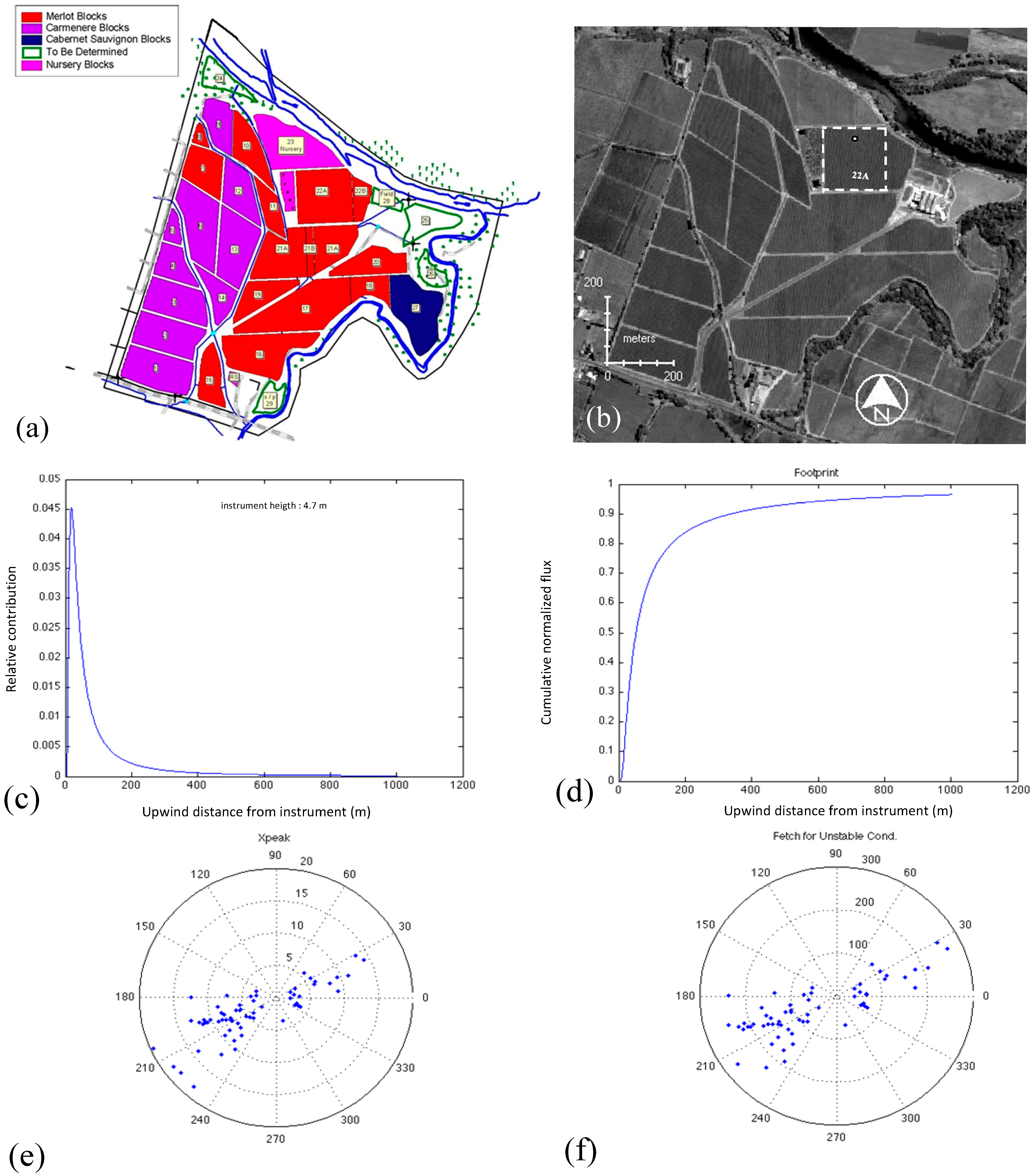
2.1. Vine Surface Energy Balance Measurements

A tower of 4.7 m of height was installed over the Merlot vineyard to measure the meteorological variables and energy balance components. Height and sensor characteristics are indicated in Table 1. To measure the net radiation, incoming (R_sin) and outgoing solar radiation (R_so) a four-component net radiometer (Kipp&Zonen Inc, CNR1, Delft, The Netherlands) was installed above the canopy. Values of R_so and R_sin were also used to compute the vineyard albedo (α = R_sin/R_so). Additionally as backup, a net radiometer (REBS, Q7.1, Seattle, WA, USA) was installed next to the tower at the same height. For the 2008–2009 seasons the four-component net radiometer was removed and the measurements continued using only the REBS Q7.1 net radiometer. Surface soil heat flux at 0.08 m depth was measured by eight soil heat flux plates (HFT3, Campbell Scientific Inc., Logan, UT, USA) regularly distributed along the space between the inter-row and inter-plant. Surface soil heat fluxes were computed by correcting the soil heat fluxes at 0.08 m using thermal storage computed from four pairs of soil temperature thermocouples (TCAV, Campbell Scientific Inc., Logan, UT, USA). These allowed the better integration of the higher values from the sun-exposed area and the lower values from the shadowed area considering the path of the sun from the morning to the afternoon.

Table 1. Sensor heights and configuration inside the experimental plot.

Sensor	Manufacturer, Model	Quantity	Heigt (m)	Origin
Four-component Net Radiometer	Kipp & Zonen, CNR1	1	4.7	Delft, The Netherlands
Net Radiometer	REBS, Q7.1	1	4.7	Washington, USA
Soil heat flux plates	Campbell Scientific, HTF3	8	−0.08	Utah, USA
Soil averaged temperature	Campbell Scientific, TCAV	4	−0.06 and −0.04	Utah, USA
Fast response open path Infrared Gas Analyzer	LI-COR Inc., LI-7500	1	4.7	Nebraska, USA
3D Sonic anemometer	Campbell Scientific, CSAT3	1	4.7	Utah, USA
Wind speed and direction	Young, 03101-5	1	4.7	Florida, USA
Air temperature and relative humidity	Vaisala, HMP45C	1	4.7	Massachusetts, USA

Table 1. Sensor heights and configuration inside the experimental plot.

Sensor	Manufacturer, Model	Quantity	Heigt (m)	Origin
Four-component Net Radiometer	Kipp & Zonen, CNR1	1	4.7	Delft, The Netherlands
Net Radiometer	REBS, Q7.1	1	4.7	Washington, USA
Soil heat flux plates	Campbell Scientific, HTF3	8	−0.08	Utah, USA
Soil averaged temperature	Campbell Scientific, TCAV	4	−0.06 and −0.04	Utah, USA
Fast response open path Infrared Gas Analyzer	LI-COR Inc., LI-7500	1	4.7	Nebraska, USA
3D Sonic anemometer	Campbell Scientific, CSAT3	1	4.7	Utah, USA
Wind speed and direction	Young, 03101-5	1	4.7	Florida, USA
Air temperature and relative humidity	Vaisala, HMP45C	1	4.7	Massachusetts, USA

Sensible and latent heat fluxes were measured using an Eddy Covariance system mounted at a height of 4.7 m (Table 1) and oriented towards the predominant wind direction (South). Sensible heat fluxes were calculated by a three-dimensional sonic anemometer/thermometer (CSAT 3, Campbell Scientific Inc., Logan, UT, USA) and latent heat fluxes were computed by a fast response open path infrared gas analyzer (IRGA) (LI-COR Inc., LI7500, Lincoln, NE, USA) as follows [46]:

LE = ρ_air · λ · w′q′

(15)

H = C_p · ρ_air · w′T′

(16)

where $\overline{\mathrm{w}\prime \mathrm{q}\prime }$ is the covariance between the instantaneous variation of the vertical wind speed (w') (m∙s−1) and humidity (q')∙(kg∙kg−1); $\overline{\mathrm{w}\prime \mathrm{T}\prime }$ is the covariance between w' and the instantaneous sonic temperature (T') (°K).

The footprint analysis indicated that 90% of cumulative normalized fluxes were close to 550 m (r_FR ≈ 117:1) at the time of satellite overpass (Figure 2c,d). Also, the wind-rose from Figure 2e,f shows the existing upwind fetch of the prevailing wind direction (South). Raw data of H and LE were post-processed considering corrections of density [47], sonic temperature [48] and coordinate rotation [49]. These data were computed over 30 min intervals. For the quality control, the energy balance closure was computed using the ratio (C_f) of turbulent fluxes (H + LE) to available energy (R_n − G). When the daily ratios were outside the range between 0.8 and 1.2, the entire day was excluded to reduce the uncertainty associated with errors in the LE and H measurements [40]. Assuming that the measurements of R_n and G were representative of the available energy in the vineyard, the fluxes of H and LE were forced to close the energy balance using the Bowen ratio [13,50,51]:

(17)

where β (= H/LE) is the hourly Bowen ratio (dimensionless). Subscript β indicates that the turbulent energy fluxes were forced to close the energy balance using the Bowen ratio.

Raw net radiation, CSAT, and IRGA data were sampled and stored in a datalogger at 10 Hz (CR5000, Campbell Scientific Inc., Logan, UT, USA). Data of the surface soil heat flux plates and soil temperature thermocouples were also sampled and stored in a separate datalogger (CR1000, Campbell Scientific Inc., Logan, UT, USA).

2.2. Reference Evapotranspiration

An automatic weather station (Adcon Telemetry, A733GSM/GPRS, Klosterneuburg, Austria) was installed over 1 ha of well-irrigated fescue grass to measure hourly variables of air temperature (T_{a_o}) (°C), relative humidity (RH_{a_o}) (%), wind speed (u₂) (m∙s⁻¹) and solar radiation (R_{sin_o}) (W∙m⁻²). This information was used to compute the reference evapotranspiration using the Penman-Monteith model [29]. The weather station was located at 6.7 km from the vineyard (35°22′ LS; 71° 35′ LW; 124 m.a.s.l.).

2.3. Ground Measurements of Vineyard Reflectance

During the growing seasons 2007–2008, 2008–2009 and 2009–2010, weekly ground measurements of reflectance for the near infrared (NIR) and red (R) wavebands (similar to Landsat) were collected for the space occupied for the canopy (r) and the bare soil (br). These measurements were taken in 64 grid points regularly spaced at 20 × 20 m² inside the experimental plot as previously indicated by [52]. The measurements of NIR and R wavebands were done using a handheld multi-spectral radiometer (CropScan Inc., MSR16R, Rochester, MN, USA). During the 2008–2009 growing season a thermal infrared thermometer (Exergen Corporation, IRt/c.2-K80F/27C,Watertown, MA, USA) was acquired to measure the thermal infrared waveband. Both sensors were mounted on a 3 m pole. Measurements were conducted near the satellite overpass time and allowed to obtain NDVI and T_s.

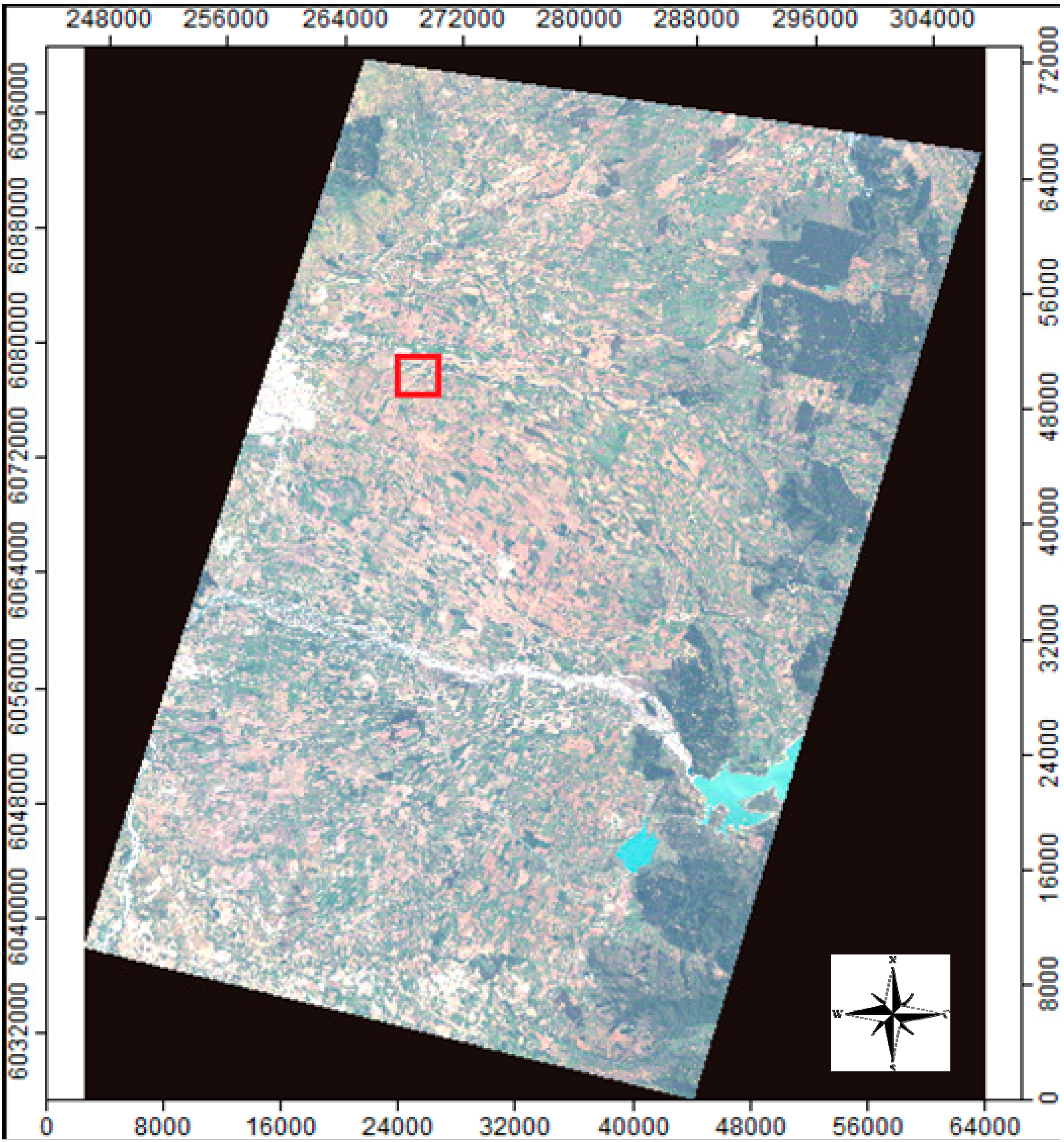
2.4. Landsat Satellite Datasets and Image Processing

Two Landsat 5 (TM) and thirteen Landsat 7 (+ETM) satellite scenes (Path 233, Row 85) were downloaded from USGS Glovis [53] (Table 2). Scenes used in this research considered only days with less than 30% cloud cover. Additionally, taking into account that since 2003 the +ETM images have shown gaps owing to failures in the satellite scan line corrector (slc-off), only scenes without gaps at the experimental plot were processed (Table 2). Maps of the complete vineyard’s surface energy balance components were drawn by using the same scenes aforementioned. All Landsat scenes used in this research were acquired including a default for the systematic radiometric and geometric corrections which consider ground control points and a Digital Elevation Model (DEM) for topographic accuracy standard terrain correction (Level 1T-precision and terrain correction) [54].

Table 2. Images selected for processing surface energy balances over a drip-irrigated Merlot vineyard.

Growing Season	Date (mm-dd-yy)	DOY *	Satellite	Overpass Time (Local Time)
2006–2007	12-29-2006	363	Landsat 7 ETM+	11:24:41
	01-12-2007	14	Landsat 7 ETM+	11:24:41
2007–2008	11-30-2007	334	Landsat 7 ETM+	11:24:47
	12-16-2007	350	Landsat 7 ETM+	11:24:47
	01-01-2008	1	Landsat 7 ETM+	11:24:49
	01-17-2008	17	Landsat 7 ETM+	11:24:49
	01-25-2008	25	Landsat 5 TM	11:25:33
	02-02-2008	33	Landsat 7 ETM+	11:24:47
	02-18-2008	49	Landsat 7 ETM+	11:24:44
2008–2009	10-23-2008	297	Landsat 5 TM	11:18:16
	11-16-2008	321	Landsat 7 ETM+	11:23:38
	12-02-2008	337	Landsat 7 ETM+	11:23:50
	01-03-2009	3	Landsat 7 ETM+	11:24:06
	02-20-2009	51	Landsat 7 ETM+	11:24:26
	03-08-2009	67	Landsat 7 ETM+	11:24:34

^* DOY = day of the year following the calendar day.

Table 2. Images selected for processing surface energy balances over a drip-irrigated Merlot vineyard.

Growing Season	Date (mm-dd-yy)	DOY *	Satellite	Overpass Time (Local Time)
2006–2007	12-29-2006	363	Landsat 7 ETM+	11:24:41
	01-12-2007	14	Landsat 7 ETM+	11:24:41
2007–2008	11-30-2007	334	Landsat 7 ETM+	11:24:47
	12-16-2007	350	Landsat 7 ETM+	11:24:47
	01-01-2008	1	Landsat 7 ETM+	11:24:49
	01-17-2008	17	Landsat 7 ETM+	11:24:49
	01-25-2008	25	Landsat 5 TM	11:25:33
	02-02-2008	33	Landsat 7 ETM+	11:24:47
	02-18-2008	49	Landsat 7 ETM+	11:24:44
2008–2009	10-23-2008	297	Landsat 5 TM	11:18:16
	11-16-2008	321	Landsat 7 ETM+	11:23:38
	12-02-2008	337	Landsat 7 ETM+	11:23:50
	01-03-2009	3	Landsat 7 ETM+	11:24:06
	02-20-2009	51	Landsat 7 ETM+	11:24:26
	03-08-2009	67	Landsat 7 ETM+	11:24:34

^* DOY = day of the year following the calendar day.

An area of study (AOS) of approximately 2804.7 km² was delimited from each satellite image (Figure 1) and several anchor pixels (cold/dry) were selected according to the method proposed in literature [27,42]. Following the selection criteria suggested by [27,42,55] several pairs of anchor pixels were used for each satellite scene. Cold pixels were located within well-known green areas inside the AOS. For hot pixels selection, several points were tested considering agricultural fields that were bare at the time of satellite overpass. Also, a spreadsheet with the two-stage slab model described in the FAO-56 manual [56] was applied to ensure the assumption that the ET_a from the soil hot pixels candidates of each image were near zero. For each image, the sensible heat flux at the cold anchor pixel was defined as it was indicated in Equation (14). In this study, a value of ϕ = 1.2 (Equation (14)) was used to estimate the H_cold considering that the ratio of reference evapotranspiration for alfalfa (ET_r) to ET_o ranges from 1.2 to 1.4 [42,57].

2.5. Calibration of LAI, z_om and G functions

It is acknowledged that originally the METRIC model was developed for annual crops and it may not apply well to sparse crops such as vineyards with low fractional cover and heterogeneous canopy. For this reason, LAI, z_om and G functions were calibrated using ground data collected from the vineyard. In this regard, the estimation of LAI was done using the Weibull function (determination coefficient (R²) = 0.85):

LAI_{_M} = 1.2 – 3.08e^{(−2013.35NDVI6.41)}

(18)

where LAI_{_M} is the Leaf Area Index modeled by satellite scene at each pixel (m²∙m⁻²)

This model was developed using values of LAI obtained from an allometric correlation [5,58] and NDVI computed from the handheld multi-spectral radiometer. It is important to indicate that values of NDVI calculated from Landsat scenes were significantly similar to those obtained from the handheld multi-spectral radiometer (R² = 0.99; MAE = 0.03; RMSE = 0.04). According to [59], the Weibull function provides good estimations of growth because it assumes a monotonically increasing sigmoid growth similar to biological systems. The flexibility of this function is attributable to the parameters showed in Equation (18): parameter 1.2 represents the upper asymptote defined as the average maximum measured LAI. The parameters 3.08 and 2013.35 are both empirical constants, which define the shape of the pattern of growth. The parameter 6.41 determines the inflexion point.

The Perrier function for estimating z_om has been suggested by other authors [27,38] as an alternative to compute z_om in sparse crops such as vineyards. In this study, values of z_om were estimated using the following calibrated function (R² = 0.96):

(19)

where h is the canopy height (m). In this regard, [12,52,60] indicated that values of the roughness length represents between 3% and 10% of plant height [12,52,60].

For soil heat flux, the calibration of Equation (8) was based on ground measurements of net radiation, soil heat flux and albedo. Also, values of NDVI and radiometric temperature were obtained using the hand-held radiometer. In this case, the calibration Equation (8) results in (R² = 0.89):

(20)

2.6. Statistical Comparison between Measured and Estimated Values

Instantaneous satellite-based estimates of momentum roughness length (z_{om_M}), leaf area index (LAI_{_M}), albedo (α_{_M}), net radiation (R_{n_M}), soil heat flux (G_{_M}), sensible heat flux (H_{_M}), and latent heat flux (LE_{_M}) were computed by averaging values of 36 (30 m × 30 m) pixels that fell within the 4.25 ha experimental plot. To avoid the “contamination” caused by pixels outside the experimental plot a perimeter of 30 m from the edges inward was excluded when calculating field-scale averages SEB fluxes [9,34,61].

The validation of sub-models that compute the instantaneous energy balance components (R_{n_M,} G_{_M}, H_{_M} and LE_{_M} ), α_{_M,} LAI_{_M} and z_{om_M} was carried out using the ratio of estimated to observed values (b), mean absolute error (MAE), root-mean-square error (RMSE) and index of agreement (d). The student’s t-test analysis was applied to check whether b was significantly different from unity at the 95% confidence level. For the validation, hourly measurements of α, R_n, G, H_β and LE_β between 1100 and 1200 h were linearly interpolated to obtain the instantaneous values (α_i, R_ni, G_i, H_βi and LE_βi) at the satellite overpass time (about 1125 h). Values of MAE, RMSE and d were respectively computed as follows [62,63,64]:

(21)

(22)

where n is the number of pairs; ${\mathrm{y}}_{\mathrm{i}}$ and $\stackrel{\wedge }{{\mathrm{y}}_{\mathrm{i}}}$ are the observed and modeled values, respectively.

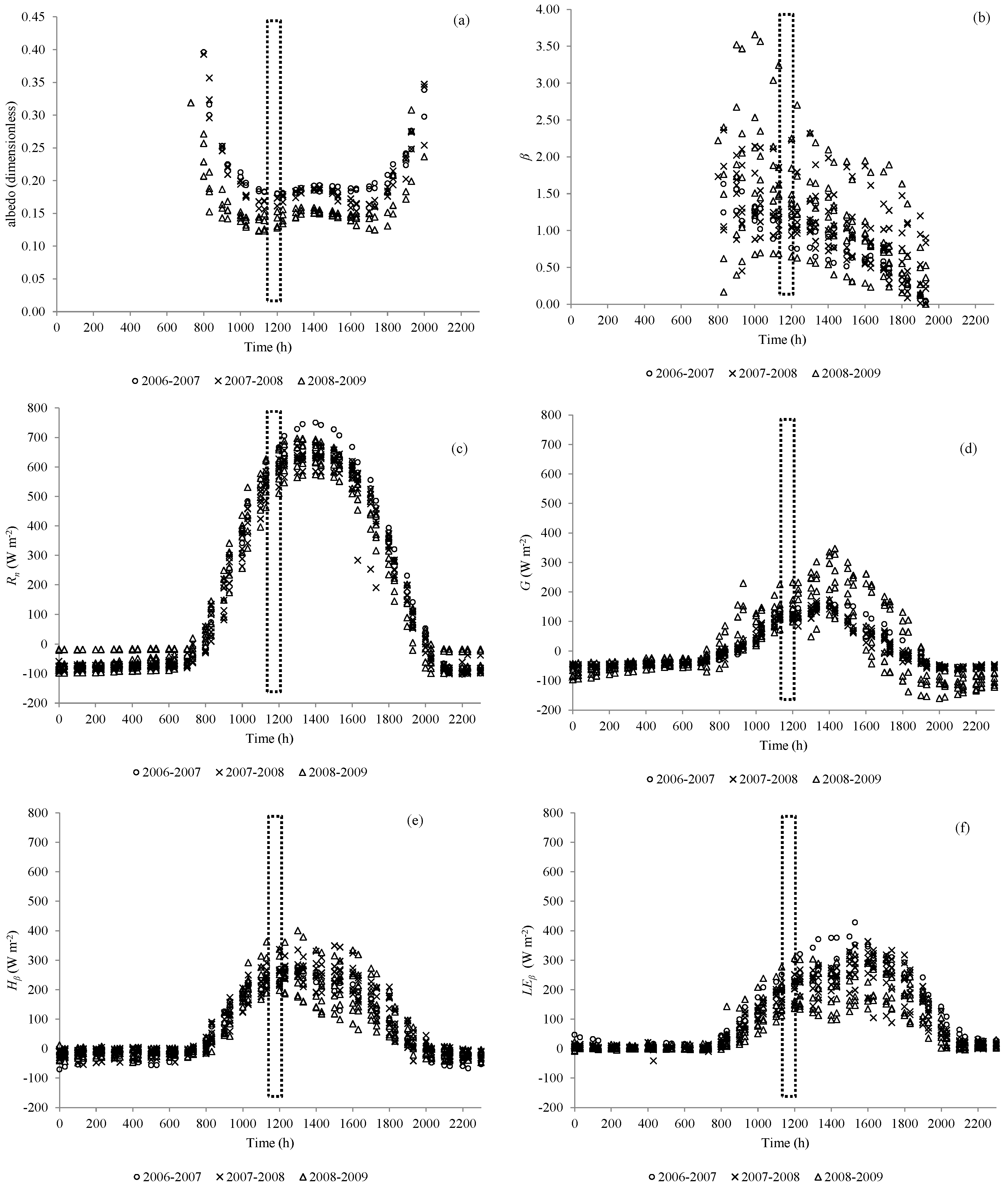
3. Results and Discussion

Generally the weather was hot and dry during the study period. Daily mean values of air temperature (T_a) and vapor pressure deficit (VPD) were 19.3 °C and 1.1 kPa, respectively. Maximum values of T_a and VPD were 35 °C and 4.1 kPa, respectively, which were reached near to 1800 h. For this study, the volumetric soil water content at rooting depth ranged from 0.25 to 0.32 m³∙m⁻³ and mean Ψ_x was between −0.4 and −1.0 MPa indicating that the Merlot vineyard was not under water stress during the three growing seasons [32,65,66,67].

The accuracy of the EC measurements above the vineyard was checked using the energy balance closure, which presented a coefficient of determination of 0.9 for the study period. Also, the hourly ratio of (H + LE) to (R_n − G) was equal to 0.9 indicating that the vineyard SEB was systematically imbalanced by about 10% [32]. On the other hand, Table 3 shows that the energy balance closure was 0.86 (±0.16) at the time of satellite overpass. According to [50], these uncertainties are modest and can be corrected using the Bowen-ratio approach (β = H/LE). In this manner, the correction of the turbulent energy fluxes increased the hourly values of latent heat flux and sensible heat fluxes by about 4% and 6%, respectively.

Table 3. Energy balance closure (C_f), Bowen ratio (β) and instantaneous ratios of latent (LE_βi), sensible (H_βi) and soil (G_i) heat fluxes to net radiation (R_ni) for a drip-irrigated vineyard at the satellite overpass. Instantaneous ratio of R_ni to incoming solar radiation (R_{sin_i}) is also included.

Season	DOY	Cf	Rni/Rsin_i	β	Hβi/Rni	LEβi/Rni	Gi/Rni
2006–2007	363	1.09	0.68	0.91	0.37	0.41	0.22
	14	0.80	0.67	1.24	0.44	0.36	0.22
2007–2008	334	0.84	0.56	1.90	0.52	0.27	0.21
	350	0.61	0.63	1.25	0.43	0.35	0.22
	1	0.88	0.58	1.09	0.41	0.38	0.21
	17	0.96	0.65	1.16	0.43	0.37	0.20
	25	0.78	0.68	1.49	0.48	0.32	0.20
	33	0.68	0.68	0.99	0.39	0.39	0.21
	49	1.01	0.76	1.18	0.41	0.35	0.24
2008–2009	297	0.76	0.66	3.17	0.63	0.20	0.17
	321	1.11	0.68	1.47	0.37	0.25	0.38
	337	0.66	0.74	1.48	0.5	0.34	0.16
	3	0.85	0.73	0.68	0.3	0.44	0.25
	51	1.08	0.71	1.89	0.48	0.25	0.27
	67	0.76	0.7	1.66	0.47	0.29	0.24
	Average	0.86	0.67	1.44	0.44	0.33	0.23
	St. Dev.	0.16	0.05	0.59	0.08	0.07	0.05

Where DOY is the day of the year. Subscript “i” denotes instantaneous values and subscript “β” denotes that the fluxes were corrected using the Bowen-ratio approach.

Table 3. Energy balance closure (C_f), Bowen ratio (β) and instantaneous ratios of latent (LE_βi), sensible (H_βi) and soil (G_i) heat fluxes to net radiation (R_ni) for a drip-irrigated vineyard at the satellite overpass. Instantaneous ratio of R_ni to incoming solar radiation (R_{sin_i}) is also included.

Season	DOY	Cf	Rni/Rsin_i	β	Hβi/Rni	LEβi/Rni	Gi/Rni
2006–2007	363	1.09	0.68	0.91	0.37	0.41	0.22
	14	0.80	0.67	1.24	0.44	0.36	0.22
2007–2008	334	0.84	0.56	1.90	0.52	0.27	0.21
	350	0.61	0.63	1.25	0.43	0.35	0.22
	1	0.88	0.58	1.09	0.41	0.38	0.21
	17	0.96	0.65	1.16	0.43	0.37	0.20
	25	0.78	0.68	1.49	0.48	0.32	0.20
	33	0.68	0.68	0.99	0.39	0.39	0.21
	49	1.01	0.76	1.18	0.41	0.35	0.24
2008–2009	297	0.76	0.66	3.17	0.63	0.20	0.17
	321	1.11	0.68	1.47	0.37	0.25	0.38
	337	0.66	0.74	1.48	0.5	0.34	0.16
	3	0.85	0.73	0.68	0.3	0.44	0.25
	51	1.08	0.71	1.89	0.48	0.25	0.27
	67	0.76	0.7	1.66	0.47	0.29	0.24
	Average	0.86	0.67	1.44	0.44	0.33	0.23
	St. Dev.	0.16	0.05	0.59	0.08	0.07	0.05

Where DOY is the day of the year. Subscript “i” denotes instantaneous values and subscript “β” denotes that the fluxes were corrected using the Bowen-ratio approach.

The hourly variation of the albedo, Bowen ratio, R_n, G, H_β and LE_β over the Merlot vineyard is presented in Figure 3. During early morning, hourly values of albedo were close to 0.4 and decreased gradually reaching an almost constant value between 1000 and 1800 h with a mean α of 0.19 (±0.05) (Figure 3a). After 1800 h, hourly albedo increased reaching values similar to those observed during early morning. At the time of satellite overpass, the measured albedo ranged from 0.12 to 0.18 for the drip-irrigated Merlot vineyard, which presented a ratio of vine row spacing (r_s) to canopy height (h_c) equal to 1.25. Using r_s/h_c = 1.6, the model of [68] estimated hourly albedos ranging between 0.18 and 0.2 for a vertical trellis system.

The diurnal variation of the Bowen ratio at the experimental plot is indicated in Figure 3b, which shows that hourly β described an almost parabolic trend skewed to the left. At the time of satellite overpass, β varied between 0.68 and 3.17 for the dataset (Table 3). Similar results were found by [69] who indicated that hourly β was between 1.25 and 0.62 for a drip-irrigated vineyard cv. Sultana trained on a T-trellis system (r_s = 3.3 m, f_c = 0.3−0.5). [46] for irrigated grapevines (h_c = 1.5 m, r_s = 2.9 m) pointed out that hourly β described an almost parabolic trend during the daytime where hourly β ranged from 0.3 to 0.75 during 1000–1700 h. Also, [70] observed values of hourly Bowen ratio between 0.2 and 0.7 during the daytime for sunny days in table grapes cv. Niagara rosada trained on vertical shoot positioned system (h_c = 1.5 m, r_s = 2.0 m).

Figure 3. Hourly variation of albedo (α), Bowen ratio (β), net radiation (R_n), soil heat flux (G), sensible heat flux (H_β) and latent heat flux (LE_β) measured above a drip-irrigated vineyard for the days when satellite scenes were available. Dotted rectangles denote the satellite overpass hour (about 1124 h). Subscript “β” denotes that the fluxes were corrected using the Bowen-ratio approach.

Figure 3. Hourly variation of albedo (α), Bowen ratio (β), net radiation (R_n), soil heat flux (G), sensible heat flux (H_β) and latent heat flux (LE_β) measured above a drip-irrigated vineyard for the days when satellite scenes were available. Dotted rectangles denote the satellite overpass hour (about 1124 h). Subscript “β” denotes that the fluxes were corrected using the Bowen-ratio approach.

Figure 3c shows that the net radiation describes a bell shaped pattern where hourly fluxes increased during the morning until reaching a peak of 650 (±44) W∙m⁻² at 1400 h. Then, R_n decreased gradually reaching values close to zero at 2000 h. Similar patterns and values of R_n were described in previous studies for vineyards [14,16,70,71,72,73]. For this study, mean ratio of R_ni to instantaneous solar radiation (R_si) was 0.67 (±0.05) at the time of satellite overpass (Table 3).

The hourly G followed a curve skewed to the right, in comparison with the shape of R_n (Figure 3d), starting at 800 h with values close to −100 W∙m⁻² and reaching at 1500 h maximum values between 100 and 400 W∙m⁻². These trends could be associated to the row orientation, canopy architecture and the soil dampness effect on the surface temperature. For the daytime (between 800 and 1800 h), the mean values of soil heat flux were 2.6 (±3) MJ∙m⁻²∙d⁻¹ which was larger than those observed by [69] (1.28 MJ∙m⁻²∙d⁻¹). For our study, values of G accounted for 11%–37% of R_n during daytime (data not shown). For this period, [12] indicated that G accounted for as much as 38%–44% of R_n for a drip irrigated Cabernet Sauvignon vineyard. Our results also differed from [7,16,69,74] who indicated that mean values of G accounted for 11%–29%, 7%–11%, 5%–8% and 9%–11% of net radiation, respectively. Differences aforementioned presumably were due to differences in canopy geometry, plant density, and the number of sensors used to compute G. Instantaneous values of G_i averaged 123 (±31) W∙m⁻² (Figure 3d) accounting for 16%–38% of R_ni.

Hourly H was small in the morning and increased near solar noon, reaching its maximum close to 400 W m⁻² between 1400 and 1500 h (Figure 3e). [16,70,73] found hourly maximum values of H between 300–400, 200–300 and 100–200 W∙m⁻², respectively. In our experiment, daytime H_β accounting for 22%–60% of R_n while [12,69] indicated that H accounted for 25%–48% of R_n. Additionally, H_βi ranged between 185 and 330 W∙m⁻² at the satellite overpass (Figure 3e). Ratios of H_βi to R_ni, were between 0.30 and 0.63 at about 1130 h, indicating that almost half of the available energy of the vineyard was dissipated into sensible heat flux at the time of satellite overpass.

Hourly value of LE_β increased smoothly from 800 h reaching its peak (400 W∙m⁻²) between 1500 and 1600 h (Figure 3f). Daytime ratio of LE_β to R_n was between 0.22 and 0.52 while the instantaneous ratio of LE_βi to R_ni was between 0.20 and 0.44. In general, results indicated that LE_β was smaller than H_β showing consistent results in comparison to previous studies carried out in a drip irrigated vineyard in the same path-row area [12] where LE accounted for 20%–40% of R_n. In this regard [69] for a drip irrigated Sultana vineyard conducted on T-trellis system (f_c = 0.4 ± 0.1) reported that the daytime ratio of LE/R_n increased from 0.43 in warm-dry periods to 0.57 in cool-humid periods. For a drip irrigated Chardonnay vineyard training on a bilateral cordon trellis, [74] indicated that the ratios of LE and H to R_n ranged between 0.46–0.67 and 0.13–0.37, respectively, concluding that the canopy architecture may have a substantial effect on soil and canopy energy balance, mainly by changing the partitioning of vineyard net irradiance into its soil and canopy components. Finally, [75] for agricultural and natural areas suggested that the partitioning of available energy is affected by water availability and vegetation cover. In our case, as aforementioned a constant shape of the canopy (a parallelepiped) was maintained without weeds between rows with LAI ranging between 0.8 and 1.2 m²∙m⁻² and f_c values of 0.3 (±0.02) during the complete evaluated periods, especially after full bloom. Also, during these seasons, the top layer of soil (0–20 cm) in the inter-rows was very dry and soil surface wetted by drip emitters was 3%. Under these canopy and soil water conditions, the soil contribution to the vineyard energy balance was considerable, especially under high atmospheric demand for water vapor. Under these conditions, sensible heat flux generated at the soil surface could be a major contributor to the vineyard energy balance which plays a key role in vine transpiration and evaporation [40].

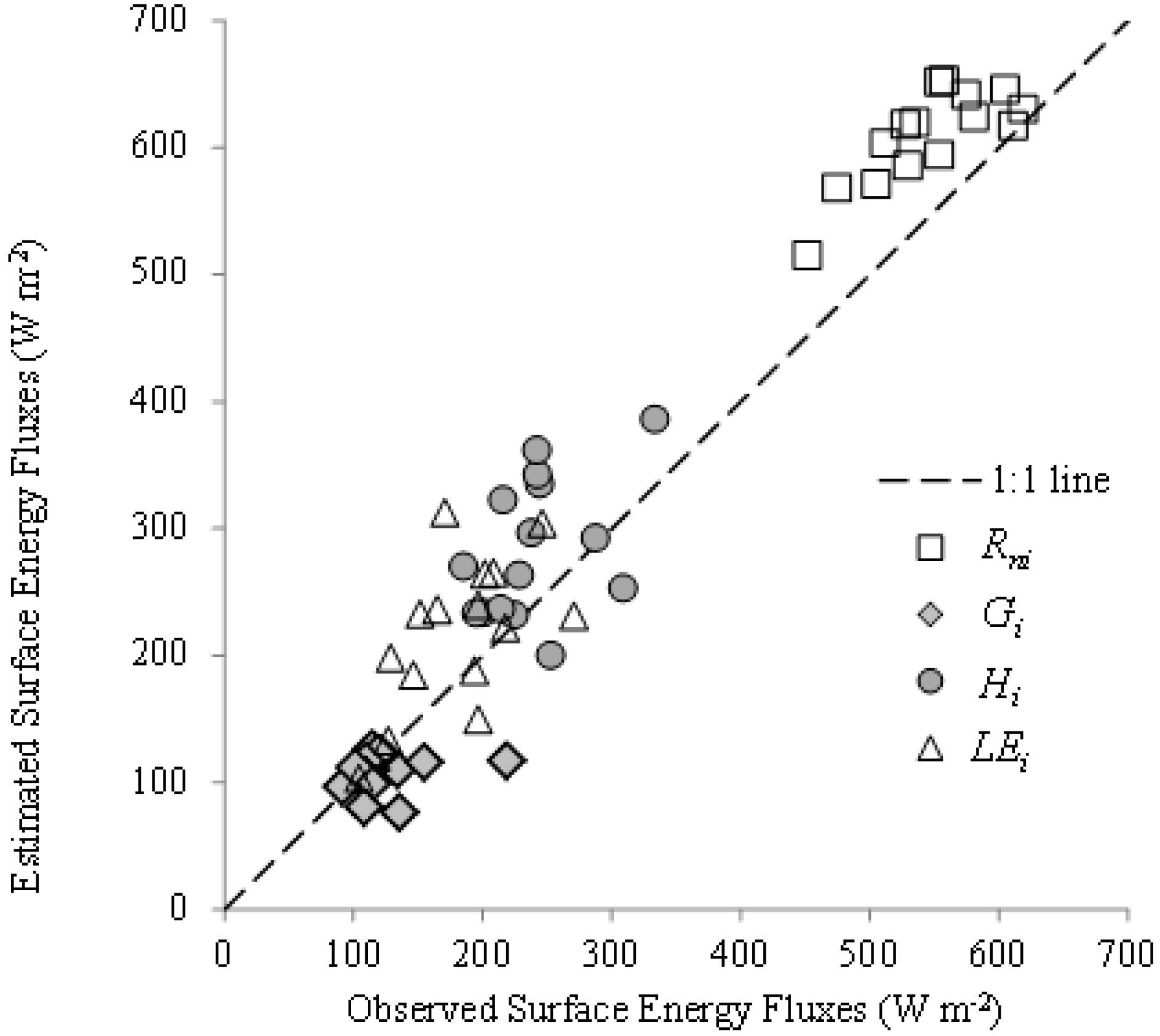
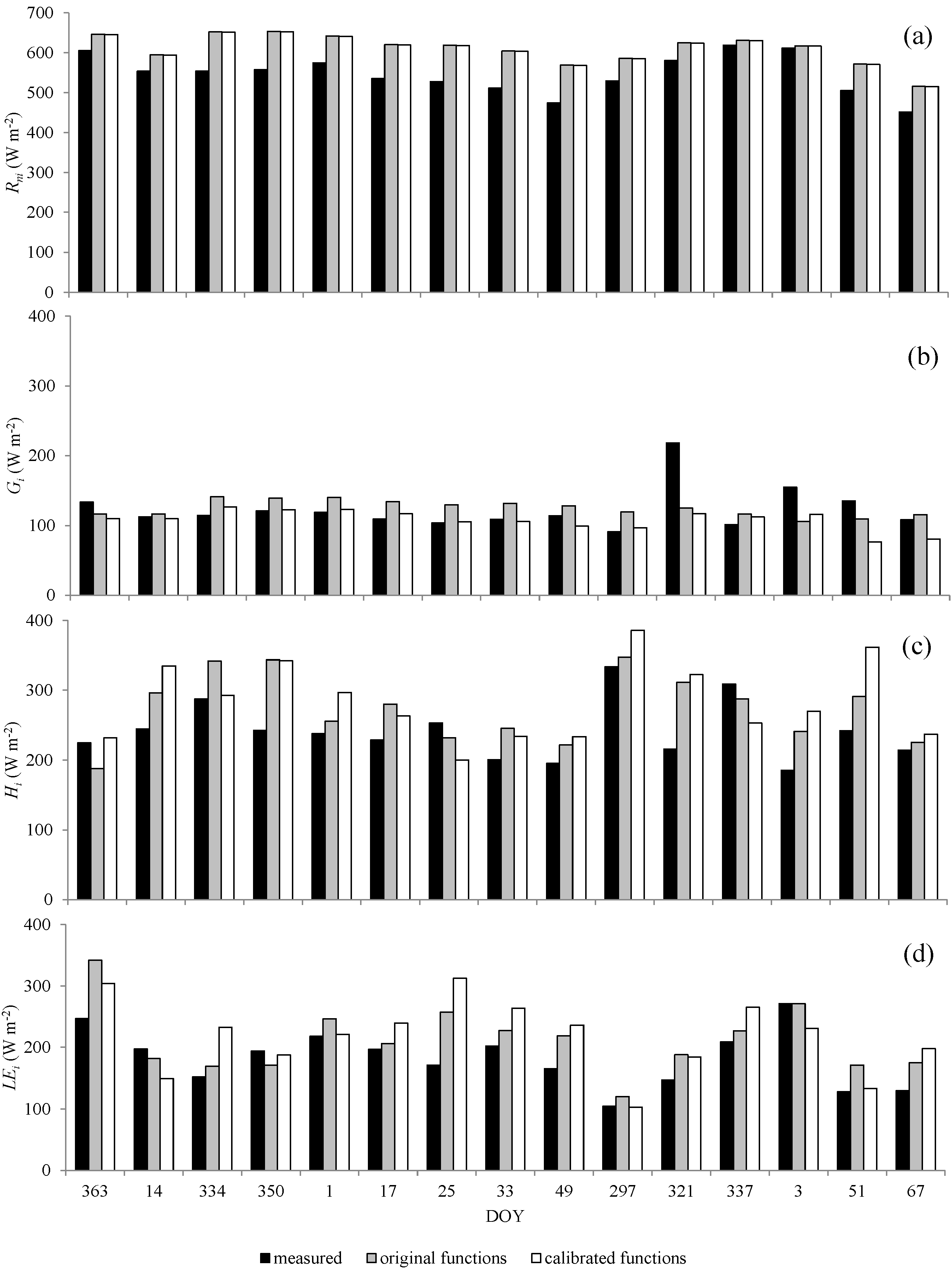
Comparison between Measured and Estimated Variables

Results showed that the Weibull model (Equation (18)) estimated LAI with values of MAE = 0.2 m²∙m⁻² and RMSE = 0.3 m²∙m⁻² (Table 4a). Also, the t-test indicated that b was significantly equal to unity indicating that estimated and observed values of LAI were similar. In contrast, the original approaches (Equations (9) and (10)) underestimated LAI by about in 58% with values of RMSE and MAE both equal to 0.6 m²∙m⁻² (Table 4b). The good results obtained with the Weibull model can be associated to the constant shape of the canopy (a parallelepiped) that was maintained with f_c values of 0.3 (±0.04) during the study period, especially after full bloom. Also, the soil surface was kept without weeds, because the top layer of soil (0–20 cm) was very dry and soil surface wetted by drip emitters was 3%. Under these constant shape and soil water conditions, NDVI may be a valid input to estimate LAI, allowing a good performance of the Weibull model. In this manner, NDVI was selected because of its simplicity and robustness against other vegetation indices based on similar studies carried out on vineyards [76,77]. On the other hand, [77] indicated that the use of NDVI computed from images of low-spatial-resolution such as Landsat (pixel resolution: 900 m²) could generate poor estimations of LAI because pixels contain mixed pixels reflectance information from the surface occupied by plants (row) and the between row space. Recently, in two vineyards, [58] indicated that the LAI can be overestimated up to 17% when contrasting geo-referenced LAI data from cover photography method against NDVI obtained from the satellite World-View 2 (pixels resolution: 2 m²).

Table 4. Validation of sub-models that compute the instantaneous values of energy balance components, albedo, leaf area index and momentum roughness length for a drip-irrigated Merlot vineyard.

(a)  Comparisons Using the Calibrated Function of LAI, zom and G
Variable	RMSE	MAE	b	d	t-Test
LAI vs. LAI_M	0.3 (m2∙m−2)	0.2 (m2∙m−2)	1.04	0.30	T
zomi vs. zom_M	0.01 (m)	0.01 (m)	0.98	0.64	T
Rni vs. Rn_M	69 (W∙m−2)	63 (W∙m−2)	1.11	0.60	F
Gi vs. G_M	34 (W∙m−2)	21 (W∙m−2)	0.83	0.39	F
Hβi vs. H_M	67 (W∙m−2)	57 (W∙m−2)	1.16	0.52	F
LEβi vs. LE_M	60 (W∙m−2)	48 (W∙m−2)	1.17	0.67	F
(b)  Comparisons Using Original Function of LAI, zom and G [27]
Variable	RMSE	MAE	b	d	t-Test
LAI vs. LAI_M	0.6 (m2∙m−2)	0.6 (m2∙m−2)	0.42	0.30	F
zomi vs. zom_M	0.08 (m)	0.08 (m)	0.19	0.50	F
αi vs. α_M	0.04	0.04	0.79	0.28	F
Rni vs. Rn_M	70 (W∙m−2)	64 (W∙m−2)	1.11	0.60	F
Gi vs. G_M	33 (W∙m−2)	26.3 (W∙m−2)	0.95	0.30	T
Hβi vs. H_M	51 (W∙m−2)	43 (W∙m−2)	1.13	0.68	F
LEβi vs. LE_M	43 (W∙m−2)	35 (W∙m−2)	1.15	0.81	F

LAI = leaf area index; z_om = momentum roughness length; α = surface albedo; R_n = net radiation; G = soil heat flux; H = sensible heat flux and LE = latent heat flux. Sub indexes “i” denotes instantaneous ground measured values, “β” denotes that the fluxes were corrected using the Bowen-ratio approach and “M” denotes modeled values using METRIC. RMSE = root mean square error; MAE = mean absolute error; b = ratio of observed to computed values; d = index of agreement; T = null hypothesis (b = 1) True; F = alternative hypothesis (b ≠ 1) False.

Table 4. Validation of sub-models that compute the instantaneous values of energy balance components, albedo, leaf area index and momentum roughness length for a drip-irrigated Merlot vineyard.

(a)  Comparisons Using the Calibrated Function of LAI, zom and G
Variable	RMSE	MAE	b	d	t-Test
LAI vs. LAI_M	0.3 (m2∙m−2)	0.2 (m2∙m−2)	1.04	0.30	T
zomi vs. zom_M	0.01 (m)	0.01 (m)	0.98	0.64	T
Rni vs. Rn_M	69 (W∙m−2)	63 (W∙m−2)	1.11	0.60	F
Gi vs. G_M	34 (W∙m−2)	21 (W∙m−2)	0.83	0.39	F
Hβi vs. H_M	67 (W∙m−2)	57 (W∙m−2)	1.16	0.52	F
LEβi vs. LE_M	60 (W∙m−2)	48 (W∙m−2)	1.17	0.67	F
(b)  Comparisons Using Original Function of LAI, zom and G [27]
Variable	RMSE	MAE	b	d	t-Test
LAI vs. LAI_M	0.6 (m2∙m−2)	0.6 (m2∙m−2)	0.42	0.30	F
zomi vs. zom_M	0.08 (m)	0.08 (m)	0.19	0.50	F
αi vs. α_M	0.04	0.04	0.79	0.28	F
Rni vs. Rn_M	70 (W∙m−2)	64 (W∙m−2)	1.11	0.60	F
Gi vs. G_M	33 (W∙m−2)	26.3 (W∙m−2)	0.95	0.30	T
Hβi vs. H_M	51 (W∙m−2)	43 (W∙m−2)	1.13	0.68	F
LEβi vs. LE_M	43 (W∙m−2)	35 (W∙m−2)	1.15	0.81	F

LAI = leaf area index; z_om = momentum roughness length; α = surface albedo; R_n = net radiation; G = soil heat flux; H = sensible heat flux and LE = latent heat flux. Sub indexes “i” denotes instantaneous ground measured values, “β” denotes that the fluxes were corrected using the Bowen-ratio approach and “M” denotes modeled values using METRIC. RMSE = root mean square error; MAE = mean absolute error; b = ratio of observed to computed values; d = index of agreement; T = null hypothesis (b = 1) True; F = alternative hypothesis (b ≠ 1) False.

Vineyard satellite-based estimations of z_om using the Perrier function (Equation (19)) generated z_om values ranging between 0.05 and 0.11 m, which are within the values indicated by [12,60]. Validation analysis indicated that RMSE and MAE where both equal to 0.01 m (Table 4a). Also, b was significantly equal to unity suggesting that estimated and observed values of z_om were similar. The original function (Equation (12)) used in METRIC algorithm [27] underestimated z_om by about 81% with RMSE and MAE both equal to 0.08 m (Table 4b). These results suggest that canopy shape and r_s/h_c ratio can plays a key role in the parameterization of z_om.

For the albedo, the statistical t-test indicated that the ratio of estimated to observed values were significantly different from the unity indicating an underestimation of 21% (Table 4b). In this case, the values of MAE and RMSE were both equal to 0.04. For the drip-irrigated vineyard, mean value of α_i was 0.2 (±0.13) while that of α_{_M} was 0.13 (±0.02). [35] indicated an albedo of 0.2 for seven sites corresponding to rainfed vineyards, which presented similar trellis structure as our experiment (r_s = 2.5 m, h_c = 1.5 m). For a non-irrigated vineyard (cv. Airen) trained on free standing bushes (f_c = 0.3, h_c = 0.9 m, r_s = 2.5), [14,60] obtained a mean albedo of 0.27 which dropped as low 0.18 during a rain event. Differences aforementioned could be associated to the training systems, r_s/h_c ratio and f_c, which affect the level of solar radiation reaching the soil surface.

Figure 4 shows the comparisons between observed and estimated values of the energy balance components at the time of satellite overpass. In this case, estimated values from METRIC were calculated using the calibrated functions of LAI, z_om and G. For the net radiation (squares) all points were over the 1:1 line with RMSE and MAE of 69.4 and 63 W∙m⁻², respectively. The t-test indicated that R_{n_M}/R_ni ratio (b =1.11) was significantly different from unity (one) indicating that METRIC overestimated R_n by approximately 11% (Table 4a). [78] showed values of RMSE and MAE equal to 51 and 25 W∙m⁻², respectively when a simplified residual SEB model was applied over a heterogeneous landscape in China. For corn, [28] reported that SEBAL overestimated R_ni by 7% with a RMSE = 65 W∙m⁻². For sorghum and corn, [79] indicated that a two-source energy balance model underestimated R_ni by about 4% with RMSE = 44.2 W∙m⁻².

The comparison between measured and modeled soil heat fluxes (diamonds) in Figure 4 shows that the points were grouped below the 1:1 line. In this case, the calibrated and original functions underestimated the instantaneous soil heat flux by about 17 and 5%, respectively, with similar values of RMSE and MAE (Table 4). Similar studies carried out by [80] indicated that METRIC estimated G_i with RMSE = 19 W∙m⁻² over a corn and soybean production region. [28] pointed out that SEBAL significantly overestimated G_i for corn with RMSE = 79.8 W∙m⁻². Also, [81] estimated the soil heat fluxes with RMSE = 23 W∙m⁻² (error of 19%) by the application of a remote sensing method overa heterogeneous surface. These authors suggested that errors could be attributable to the difference of spatial/temporal scales between satellite data and measurements.

The comparison between measured and estimated sensible heat fluxes during satellite overpasses (Figure 4–circles) shows that the points were over the 1:1 line. In this case, METRIC using the calibrated functions of LAI, z_om and G overestimates the instantaneous sensible heat fluxes by about 16% with RMSE, MAE and d equal to 67 W∙m⁻², 57 W∙m⁻² and 0.52, respectively (Table. 4a). When using the original function, METRIC overestimated the instantaneous sensible heat fluxes by about 13% (RMSE = 51 W∙m⁻²; MAE = 43 W∙m⁻² and d = 0.68) (Table 4b). For corn and soybean, [80] indicated that METRIC tends to overestimate H_i by about 80 W∙m⁻² with RMSE = 57 W∙m⁻². For corn, [28] indicated that instantaneous values of H were underestimated by nearly 50%. Over heterogeneous surfaces [78] indicated that the RMSE was 23 W∙m⁻² when a simplified residual SEB model was applied to estimate the sensible heat flux at the time of satellite overpass. According to [26,44,82], biases in the estimation of sensible heat fluxes are necessary because calculations (iterations) of H_{_M} absorb the biases obtained previously in the computation of net radiation and soil heat fluxes. As a consequence the accuracy of the complete model in the estimation of LE_{_M} strongly depends on the anchor pixel selection (end members), which determines the self-calibration of H_{_M}.

Figure 4. Comparisons at the time of satellite overpass between observed (axis X) and estimated (axis Y) values of net radiation (R_n), soil heat flux (G), sensible heat flux (H), and latent heat flux (LE) for a drip irrigated Merlot vineyard. Estimated values were obtained using METRIC with the calibrated functions. Subscript “i” denotes instantaneous values.

Figure 4. Comparisons at the time of satellite overpass between observed (axis X) and estimated (axis Y) values of net radiation (R_n), soil heat flux (G), sensible heat flux (H), and latent heat flux (LE) for a drip irrigated Merlot vineyard. Estimated values were obtained using METRIC with the calibrated functions. Subscript “i” denotes instantaneous values.

For the instantaneous latent heat flux, Figure 4 (triangles) depicts an equilibrated distribution of points around the 1:1 line with RMSE and MAE equal to 60 and 48 W∙m⁻², respectively (Table 4a). When using the calibrated functions, the ratio of LE_{_M}/LE_i was significantly different to the unity suggesting that instantaneous values of LE_{_M} were overestimated by about in 17%. When using original functions, METRIC significantly overestimated (15%) the latent heat flux over the drip-irrigated vineyard with values of RMSE, MAE and d equal to 43, 35 W∙m⁻² and 0.8, respectively (Table 4b). For drip-irrigated vineyards, [83] found errors of 18% in the estimation of LE_i when using a two-source energy balance (TSEB) model and Landsat scenes. In spite of this error, the TSEB model estimated daily ET_a with RMSE equal to 0.5 mm∙d⁻¹. In this regard, [32] observed that errors of 15% in the estimation of LE_i produced an ET_a overestimation of 9% with a RMSE = 0.62 mm∙d⁻¹ for the same Merlot vineyard. For fully covered crops, [28,80] found values of RMSE equal to 108 in corn and 55 W∙m⁻² in soybean, respectively. In general, the literature indicates that most of the remote sensing models applied over full or sparse canopies to estimate daily ET_a presented errors between 0.5 and 0.8 mm∙d⁻¹ which are acceptable for irrigation management [22,35,83].

METRIC with original (grey bars) and calibrated (white bars) functions both overestimated the instantaneous net radiation by about 63 (±30) W∙m⁻² during the growing cycle (Figure 5a). In this regard, the calibrated function of LAI did not produce a significant effect on the computation of the surface emissivities, which are used by METRIC to estimate the outgoing long wave radiation and surface temperature [27]. Values of H_{_M}, LE_{_M} and G_{_M} using the calibrated functions showed biases of 35 (±50), 43 (±53) and −15 (±31) W∙m⁻², respectively; while those using the original functions presented biases of 29 (±33), 33 (±40) and 2 (±35) W∙m⁻², respectively. These results suggest that errors in the estimation of LAI_{_M}, z_{om_M} and G_{_M} were balanced by the self-calibration of METRIC to estimate the instantaneous turbulent energy fluxes. Also, errors in estimations of R_ni (Figure 5a) and G_i (Figure 5b) were typically balanced by bias in H_i (Figure 5c). This buffer effect significantly influenced the estimations of latent heat fluxes at the time of satellite overpasses (Figure 5d).

Figure 5. Comparisons between the measured (black bars) and modeled values using METRIC with the original (grey bars) and calibrated (white bars) functions to estimate (a) net radiation (R_ni); (b) soil heat flux (G_i); (c) sensible heat flux (H_i); and (d) latent heat flux (LE_i) at the time of satellite overpass. Modeled values correspond to average from pixels inside the experimental plot. DOY is the day of the year. Subscript “i” denotes instantaneous values.

Figure 5. Comparisons between the measured (black bars) and modeled values using METRIC with the original (grey bars) and calibrated (white bars) functions to estimate (a) net radiation (R_ni); (b) soil heat flux (G_i); (c) sensible heat flux (H_i); and (d) latent heat flux (LE_i) at the time of satellite overpass. Modeled values correspond to average from pixels inside the experimental plot. DOY is the day of the year. Subscript “i” denotes instantaneous values.

In this respect, sensitivity analysis studies applied to METRIC model indicated that variations on intermediate parameters (albedo, NDVI, LAI, G and roughness length) indirectly could affect the accuracy of LE_i and subsequently ET_a estimation [84,85], but the most important effect is attributable to the end member selection [82,85,86,87,88,89]. On this point, [90] indicated that the spatial distribution of H_i in the image is based on H_i estimation between two anchor pixels. So, if LE_i at the anchor pixel is overestimated then H will be underestimated throughout the satellite scene. On the contrary, if LE_i is underestimated, H_i will be overestimated. According to [27] the selection of the two “anchor” pixels requires knowledge, thoughtfulness and skill of the operator. These points have been indicated as controversial inside the ET research community because selection is subjective and depends of the ability of the operator in search and isolate of the most appropriates hot and cold pixels [55,87,88].

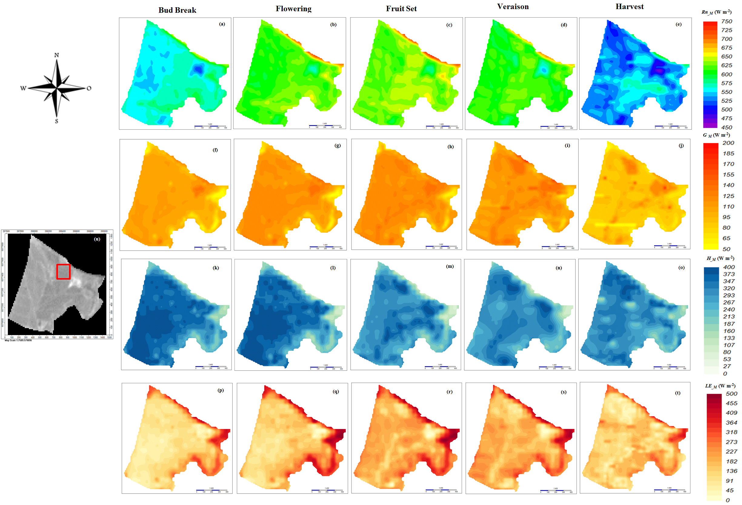
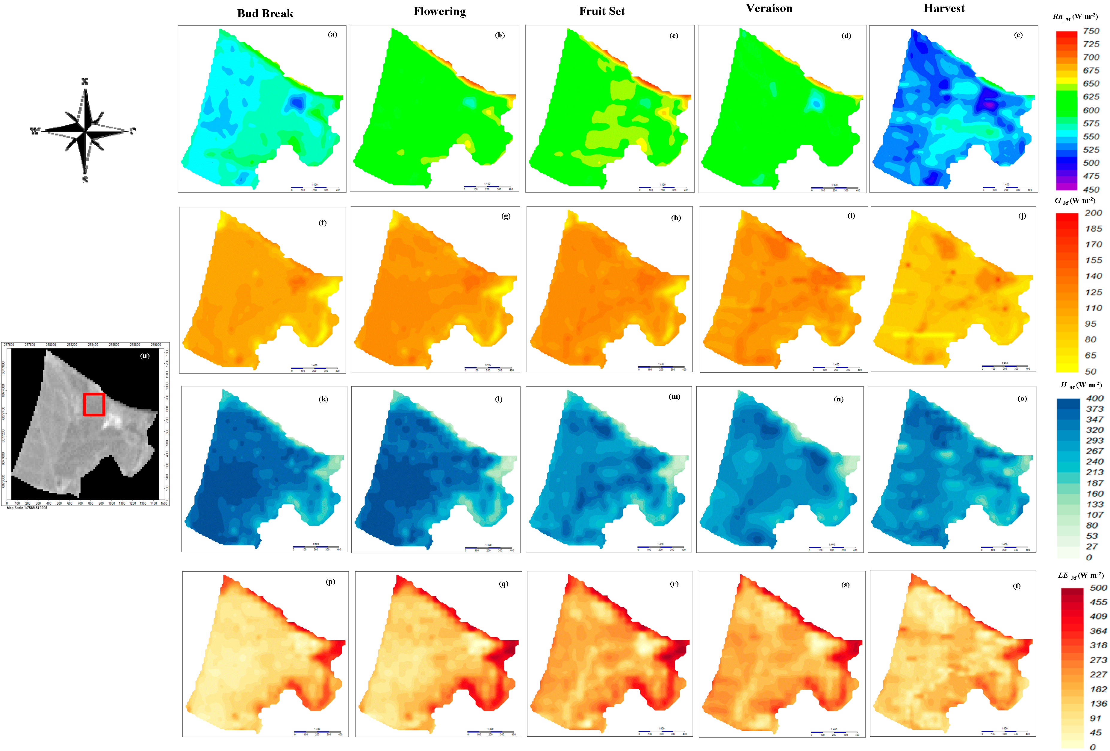
Spatial Variability of the Estimated Surface Energy Balance Components for the Complete Vineyard

At the time of satellite overpass, Figure 6 shows the maps with the spatial variability of the satellite-based energy balance components estimated by METRIC using the calibrated functions. For the entire vineyard (97 ha), the maps were generated for the phenological stages of bud break (B), flowering (FL), fruit set (FS), veraison (V) and harvest (HA). Average values of R_{n_M} for the pixels inside the vineyard were 565 (±16), 565 (±16), 619 (±17), 632 (±17), 613 (±15) and 537 (±17) W∙m⁻² for B, FL, FS, V and HA, respectively (Figure 6a–e). In this case, the coefficient of variation (less than 5%) indicated that the spatial variability of R_{n_M} was not important. For B, FL, FS, V and HA G_{_M} ranged between 50 and 190 W∙m⁻² with maximum and minimum values observed in veraison and fruit set, respectively (Figure 6f–j). Average values of H_{_M} were 326 (±64), 311 (±78), 280 (±63), 281 (±59) and 296 (±44) W∙m⁻² (Figure 6k–o) while those of LE_{_M} were 135 (±86), 180 (±98), 223 (±81), 209 (±76) and 155 (±70) W∙m⁻² (Figure 6p–t) for B, FL, FS, V and HA, respectively. In Figure 6k-o nearly a third of the complete vineyard can be clearly identified inside a dark blue area (387 W∙m⁻²) corresponding to the old part of the vineyard where the training system shown more separated vines than the described for Merlot occupied in this study. The effect of distance inside this area presumably could increase the sensible heat flux due the bare soil beneath vines, considering that during this period the vineyard did not reach its complete foliage cover. Also, the highest and lowest values of H_{_M} (400 W∙m⁻²) and LE_{_M} (30 W∙m⁻²) were observed in areas without plants (bare soil and winery). The highest values of R_{n_M} (726 W∙m⁻²) and LE_{_M} (300–500∙W m⁻²) were observed in the vineyard contours reflecting the presence of trees, natural bushes and the influence of the “Lircay” River. The low spatial variability of G_{_M}, H_{_M} and LE_{_M} observed for each phenological stage was associated with the uniform canopy shape of the vineyard where the values of LAI and fractional cover (f_c) were maintained between 0.8–1.2 m²∙m⁻² and 0.28–0.31, respectively, particularly after the full bloom soil surface was very dry and maintained free of weeds (cover crops) during October and March for all evaluation period in which rainfall was less than 3.0 (±2.4) mm.

Figure 6. Averaged spatial distribution of net radiation (R_{n_M}) (a–e); soil heat flux (G_{_M}) (f–j); sensible heat flux (H_{_M}) (Figure k–o); and latent heat flux (LE_{_M}) (p–t) over a drip-irrigated vineyard computed by the calibrated METRIC model. Column headers indicate the phenological stages. Averages were done combining data from the 2006–2007, 2007–2008 and 2008–2009 growing seasons; A panchromatic scene (u) from Landsat 7 (ETM+; DOY 17, 2008) is included as reference. The red square indicates the experimental plot location.

Figure 6. Averaged spatial distribution of net radiation (R_{n_M}) (a–e); soil heat flux (G_{_M}) (f–j); sensible heat flux (H_{_M}) (Figure k–o); and latent heat flux (LE_{_M}) (p–t) over a drip-irrigated vineyard computed by the calibrated METRIC model. Column headers indicate the phenological stages. Averages were done combining data from the 2006–2007, 2007–2008 and 2008–2009 growing seasons; A panchromatic scene (u) from Landsat 7 (ETM+; DOY 17, 2008) is included as reference. The red square indicates the experimental plot location.

4. Conclusions

Empirical functions of METRIC to estimate LAI, z_om and G_i were calibrated for a drip-irrigated vineyard under non-water stress (midday Ψx > −1.0 MPa). Results indicated that LAI, z_om and G_i were estimated using the calibrated functions with errors of 4%, 2% and 17% while those were computed using the original functions with errors of 58%, 81%, and 21%, respectively. At the time of satellite overpass, the original METRIC underestimated the satellite-based albedo by about 21% and overestimated net radiation by 11%. Using the calibrated functions, METRIC overestimated instantaneous latent and sensible heat fluxes by about 17% and 16%, respectively. Using the original functions, it overestimated LE and H with errors of 15% and 13%, respectively. Results of this research indicated that the calibration of G_i, LAI and z_om did not produce significant effects on the estimation of the turbulent energy fluxes because of the self-calibration employed in the estimation of H_{_M}. Also, biases observed for instantaneous pixel-by-pixel values of R_{n_M} and G_{_M}, were presumably absorbed into H_{_M} as a result of the self-calibration method of METRIC, which is highly dependent on the hot and cold pixels selection. Finally, future research needs to be performed considering a sensitivity analysis of intermediate variables and the use of an automatized method to optimize the selection of anchor pixels (wet and dry) at each scene.

References

1. Costa, J.M.; Ortuno, M.F.; Chaves, M.M. Deficit irrigation as a strategy to save water: Physiology and potential application to horticulture. J. Integr. Plant Biol. 2007, 49, 1421–1434. [Google Scholar] [CrossRef]
2. Chaves, M.M.; Santos, T.P.; Souza, C.R.; Ortuño, M.F.; Rodrigues, M.L.; Lopes, C.M.; Maroco, J.P.; Pereira, J.S. Deficit irrigation in grapevine improves water-use efficiency while controlling vigour and production quality. Ann. Appl. Biol. 2007, 150, 237–252. [Google Scholar] [CrossRef]
3. Fereres, E.; Soriano, M.A. Deficit irrigation for reducing agricultural water use. J. Exp. Bot. 2007, 58, 147–159. [Google Scholar] [CrossRef] [PubMed]
4. Williams, L.E.; Matthews, M.A. Grapevine. In Irrigation of Agricultural Crops–Agronomy Monograph; Stewart, B.A., Nielson, D.R., Eds.; ASA-CSSA-SSSA: Madison, WI, USA, 1990; Volume 30; pp. 1019–1059. [Google Scholar]
5. Poblete-Echeverria, C.; Ortega-Farias, S. Estimation of actual evapotranspiration for a drip-irrigated Merlot vineyard using a three-source model. Irrig. Sci. 2009, 28, 65–78. [Google Scholar] [CrossRef]
6. Ferreyra, R.; Selles, V.; Peralta, J.; Burgos, L.; Valenzuela, J. Efectos de la restricción del riego en distintos períodos de desarrollo de la vid cv. Cabernet sauvignon sobre producción y calidad del vino. Agric. Tec. 2002, 62, 406–417. [Google Scholar]
7. Trambouze, W.; Bertuzzi, P.; Voltz, M. Comparison of methods for estimating actual evapotranspiration in a row-cropped vineyard. Agric. For. Meteorol. 1998, 91, 193–208. [Google Scholar] [CrossRef]
8. Anderson, M.C.; Norman, J.M.; Mecikalski, J.R.; Otkin, J.A.; Kustas, W.P. A climatological study of evapotranspiration and moisture stress across the continental United States based on thermal remote sensing: 1. Model formulation. J. Geophys. Res. Atmos. 2007, 112, D10117. [Google Scholar] [CrossRef]
9. Bastiaanssen, W.G.M.; Menenti, M.; Feddes, R.A.; Holtslag, A.A.M. A remote sensing surface energy balance algorithm for land (SEBAL)—1. Formulation. J. Hydrol. 1998, 213, 198–212. [Google Scholar] [CrossRef]
10. Verstraeten, W.W.; Veroustraete, F.; Feyen, J. Assessment of evapotranspiration and soil moisture content across different scales of observation. Sensors 2008, 8, 70–117. [Google Scholar] [CrossRef]
11. Steiner, J.L.; Hatfield, J.L. Winds of change: A century of agroclimate research. Agron. J. 2008, 100, S132–S152. [Google Scholar] [CrossRef]
12. Ortega-Farias, S.; Carrasco, M.; Olioso, A.; Acevedo, C.; Poblete, C. Latent heat flux over Cabernet Sauvignon vineyard using the Shuttleworth and Wallace model. Irrig. Sci. 2007, 25, 161–170. [Google Scholar] [CrossRef]
13. Balbontin-Nesvara, C.; Calera-Belmonte, A.; Gonzalez-Piqueras, J.; Campos-Rodriguez, I.; Lopez-Gonzalez, M.L.; Torres-Prieto, E. Vineyard evapotranspiration measuraments in a semiarid environment: Eddy covariance and bowen ratio comparison. Agrociencia 2010, 45, 87–103. [Google Scholar]
14. Oliver, H.R.; Sene, K.J. Energy and water balances of developing vines. Agric. For. Meteorol. 1992, 61, 167–185. [Google Scholar] [CrossRef]
15. Heilman, J.L.; McInnes, K.J.; Savage, M.J.; Gesch, R.W.; Lascano, R.J. Soil and canopy energy balances in a west Texas vineyard. Agric. For. Meteorol. 1994, 71, 99–114. [Google Scholar] [CrossRef]
16. Kordova-Biezuner, L.; Mahrer, I.; Schwartz, C. Estimation of actual evapotranspiration from vineyard by utilizing eddy correlation method. Acta Hortic. 2000, 537, 167–175. [Google Scholar]
17. Campos, I.; Neale, C.M.U.; Calera, A.; Balbontín, C.; González-Piqueras, J. Assessing satellite-based basal crop coefficients for irrigated grapes (Vitis vinifera L.). Agric. Water Manag. 2010, 98, 45–54. [Google Scholar] [CrossRef]
18. Kleissl, J.; Hong, S.H.; Hendrickx, J.M.H. New Mexico scintillometer network supporting remote sensing and hydrologic and meteorological models. Bull. Am. Meteorol. Soc. 2009, 90. [Google Scholar] [CrossRef]
19. Gowda, P.H.; Chávez, J.L.; Colaizzi, P.D.; Evett, S.R.; Howell, T.A.; Tolk, J.A. Remote sensing based energy balance algorithms for mapping ET: Current status and future challenges. Trans. ASABE 2007, 50, 1639–1644. [Google Scholar] [CrossRef]
20. Allen, R.G.; Pereira, L.S.; Howell, T.A.; Jensen, M.E. Evapotranspiration information reporting: I. Factors governing measurement accuracy. Agric. Water Manag. 2011, 98, 899–920. [Google Scholar] [CrossRef]
21. Courault, D.; Seguin, B.; Olioso, A. Review on estimation of evapotranspiration from remote sensing data: From empirical to numerical modeling approaches. Irrig. Drain. Syst. 2005, 19, 223–249. [Google Scholar] [CrossRef]
22. Kalma, J.; McVicar, T.; McCabe, M. Estimating land surface evaporation: A review of methods using remotely sensed surface temperature data. Surv. Geophys. 2008, 29, 421–469. [Google Scholar] [CrossRef]
23. Santos, C.; Lorite, I.J.; Tasumi, M.; Allen, R.G.; Fereres, E. Performance assessment of an irrigation scheme using indicators determined with remote sensing techniques. Irrig. Sci. 2010, 28, 461–477. [Google Scholar] [CrossRef]
24. Gowda, P.; Chavez, J.; Colaizzi, P.; Evett, S.; Howell, T.; Tolk, J. ET mapping for agricultural water management: Present status and challenges. Irrig. Sci. 2008, 26, 223–237. [Google Scholar] [CrossRef]
25. Seguin, B.; Courault, D.; Guérif, M. Surface temperature and evapotranspiration: Application of local scale methods to regional scales using satellite data. Remote Sens. Environ. 1994, 49, 287–295. [Google Scholar] [CrossRef]
26. Allen, R.G.; Tasumi, M.; Morse, A.; Trezza, R.; Wright, J.L.; Bastiaanssen, W.; Kramber, W.; Lorite, I.; Robison, C.W. Satellite-based energy balance for mapping evapotranspiration with internalized calibration (METRIC) applications. J. Irrig. Drain. Eng. 2007, 133, 395–406. [Google Scholar] [CrossRef]
27. Allen, R.G.; Tasumi, M.; Trezza, R.; Kjaersgaard, J.H. METRIC—Mapping Evapotranspiration at High Resolution, Application Manual. Available online: http://www.kimberly.uidaho.edu/water/metric/index.html (accessed on 30 May 2014).
28. Singh, R.K.; Irmak, A.; Irmak, S.; Martin, D.L. Application of SEBAL model for mapping evapotranspiration and estimating surface energy fluxes in South-Central Nebraska. J. Irrig. Drain. Eng. 2008, 134, 273–285. [Google Scholar] [CrossRef]
29. ASCE-EWRI. The ASCE standarized reference evapotranspiration equation. In Report of the ASCE-EWRI Task Committee on Standarization of Reference Evapotranspiration; ASCE-EWRI: Kimberly, ID, USA, 2005; p. 147. [Google Scholar]
30. Allen, R.G.; Tasumi, M.; Trezza, R. Satellite-based energy balance for mapping evapotranspiration with internalized calibration (METRIC) Model. J. Irrig. Drain. Eng. 2007, 133, 380–394. [Google Scholar] [CrossRef]
31. Chávez, J.; Neale, C.; Prueger, J.; Kustas, W. Daily evapotranspiration estimates from extrapolating instantaneous airborne remote sensing ET values. Irrig. Sci. 2008, 27, 67–81. [Google Scholar] [CrossRef]
32. Carrasco-Benavides, M.; Ortega-Farías, S.; Lagos, L.O.; Kleissl, J.; Morales, L.; Poblete-Echeverría, C.; Allen, R. Crop coefficients and actual evapotranspiration of a drip-irrigated Merlot vineyard using multispectral satellite images. Irrig. Sci. 2012, 1–13. [Google Scholar]
33. Allen, R.; Irmak, A.; Trezza, R.; Hendrickx, J.M.H.; Bastiaanssen, W.; Kjaersgaard, J. Satellite-based ET estimation in agriculture using SEBAL and METRIC. Hydrol. Proc. 2011, 25, 4011–4027. [Google Scholar] [CrossRef]
34. Tasumi, M.; Allen, R.G.; Trezza, R.; Wright, J.L. Satellite-based energy balance to assess within-population variance of crop coefficient curves. J. Irrig. Drain. Eng. 2005, 131, 94–109. [Google Scholar] [CrossRef]
35. Galleguillos, M.; Jacob, F.; Prévot, L.; French, A.; Lagacherie, P. Comparison of two temperature differencing methods to estimate daily evapotranspiration over a Mediterranean vineyard watershed from ASTER data. Remote Sens. Environ. 2011, 115, 1326–1340. [Google Scholar] [CrossRef]
36. Galleguillos, M.; Jacob, F.; Prevot, L.; Lagacherie, P.; Liang, S.L. Mapping daily evapotranspiration over a mediterranean vineyard watershed. IEEE Geosci. Remote Sens. Lett. 2011, 8, 168–172. [Google Scholar] [CrossRef]
37. Bastiaanssen, W.G.M.; Pelgrum, H.; Soppe, R.W.O.; Allen, R.G.; Thoreson, B.P.; Teixeira, A.H. Thermal-infrared technology for local and regional scale irrigation analyses in horticultural systems. Acta Hortic. 2008, 793, 33–46. [Google Scholar]
38. Santos, C.; Lorite, I.J.; Allen, R.G.; Tasumi, M. Aerodynamic parameterization of the satellite-based energy balance (METRIC) model for ET estimation in rainfed olive orchards of Andalusia, Spain. Water Resour. Manag. 2012, 26, 3267–3283. [Google Scholar] [CrossRef]
39. Teixeira, A.H.; Bastiaanssen, W.G.M.; Ahmad, M.D.; Bos, M.G. Reviewing SEBAL input parameters for assessing evapotranspiration and water productivity for the Low-Middle Sao Francisco River basin, Brazil Part B: Application to the regional scale. Agric. For. Meteorol. 2009, 149, 477–490. [Google Scholar] [CrossRef]
40. Ortega-Farias, S.; Poblete-Echeverría, C.; Brisson, N. Parameterization of a two-layer model for estimating vineyard evapotranspiration using meteorological measurements. Agric. For. Meteorol. 2010, 150, 276–286. [Google Scholar] [CrossRef]
41. Tasumi, M.; Allen, R.G.; Trezza, R. At-surface reflectance and albedo from satellite for operational calculation of land surface energy balance. J. Hydrol. Eng. 2008, 13, 51–63. [Google Scholar] [CrossRef]
42. Tasumi, M. Progress in Operational Estimation of Regional Evapotranspiration Using Satellite Imagery. Ph.D. Thesis, University of Idaho, Moscow, ID, USA, 2003. [Google Scholar]
43. Basso, B.; Cammarano, D.; DeVita, P. Remotely sensed vegetation indices: Theory and applications for crop management. Riv. Ital. Agrometeorol. 2004, 1, 36–53. [Google Scholar]
44. Kjaersgaard, J.H.; Allen, R.G.; Garcia, M.; Kramber, W.; Trezza, R. Automated selection of anchor pixels for landsat based evapotranspiration estimation. In World Environmental and Water Resources Congress 2009 Great Rivers; ASCE, Ed.; ASCE: Kansas City, MO, USA, 2009; pp. 4400–4410. [Google Scholar]
45. Coombe, B.G. Growth Stages of the Grapevine: Adoption of a system for identifying grapevine growth stages. Aust. J. Grape Wine Res. 1995, 1, 104–110. [Google Scholar] [CrossRef]
46. Li, S.; Tong, L.; Li, F.; Zhang, L.; Zhang, B.; Kang, S. Variability in energy partitioning and resistance parameters for a vineyard in northwest China. Agric. Water Manag. 2009, 96, 955–962. [Google Scholar] [CrossRef]
47. Webb, E.; Pearman, G.; Leuning, R. Correction of flux measurements for density effects due to heat and water vapour transfer. Q. J. R. Meteorol. Soc. 1980, 106, 85–100. [Google Scholar] [CrossRef]
48. Schotanus, P.; Nieuwstadt, F.T.M.; de Bruin, H.A.R. Temperature measurement with a sonic anemometer and its application to heat and moisture fluctuations. Bound. Layer Meteorol. 1983, 26, 81–93. [Google Scholar] [CrossRef]
49. Wilczak, J.; Oncley, S.; Stage, S. Sonic anemometer tilt correction algorithms. Bound. Layer Meteorol. 2001, 99, 127–150. [Google Scholar] [CrossRef]
50. Twine, T.E.; Kustas, W.P.; Norman, J.M.; Cook, D.R.; Houser, P.R.; Meyers, T.P.; Prueger, J.H.; Starks, P.J.; Wesely, M.L. Correcting eddy-covariance flux underestimates over a grassland. Agric. For. Meteorol. 2000, 103, 279–300. [Google Scholar] [CrossRef]
51. Chávez, J.; Howell, T.; Copeland, K. Evaluating eddy covariance cotton ET measurements in an advective environment with large weighing lysimeters. Irrig. Sci. 2009, 28, 35–50. [Google Scholar] [CrossRef]
52. Poblete-Echeverría, C.; Ortega-Farias, S. Calibration and validation of a remote sensing algorithm to estimate energy balance components and daily actual evapotranspiration over a drip-irrigated Merlot vineyard. Irrig. Sci. 2012, 30, 537–553. [Google Scholar] [CrossRef]
53. Earth Resources Observation and Science Center (EROS). USGS Global Visualization Viewer. Available online: http://glovis.usgs.gov/ (accessed on 1 September 2010).
54. Earth Resources Observation and Science Center (EROS). Landsat Processing Details. Available online: http://landsat.usgs.gov/Landsat_Processing_Details.php (accessed on 22 July 2014).
55. Cuenca, R.; Ciotti, S.; Hagimoto, Y. Application of landsat to evaluate effects of irrigation forbearance. Remote Sens. 2013, 5, 3776–3802. [Google Scholar] [CrossRef]
56. Allen, R.G.; Pereira, L.S.; Raes, D.; Smith, M. FAO irrigation and drainage paper No. 56. In Crop Evapotranspiration Guidelines for Computing Crop Water Requirements; Food and Agriculture Organization of the United Nations: Rome, Italy, 1998; p. 298. [Google Scholar]
57. Folhes, M.T.; Renno, C.D.; Soares, J.V. Remote sensing for irrigation water management in the semi-arid Northeast of Brazil. Agric. Water Manag. 2009, 96, 1398–1408. [Google Scholar] [CrossRef]
58. Fuentes, S.; Poblete-Echeverría, C.; Ortega-Farias, S.; Tyerman, S.; de Bei, R. Automated estimation of leaf area index from grapevine canopies using cover photography, video and computational analysis methods. Aust. J. Grape Wine Res. 2014, 20, 465–473. [Google Scholar] [CrossRef]
59. Yang, R.C.; Kozak, A.; Smith, J.H.G. The potential of Weibull-type functions as flexible growth curves. Can. J. For. Res. 1978, 8, 424–431. [Google Scholar]
60. Sene, K.J. Parameterisations for energy transfers from a sparse vine crop. Agric. For. Meteorol. 1994, 71, 1–18. [Google Scholar] [CrossRef]
61. Singh, R.K.; Irmak, A. Estimation of crop coefficients using satellite remote sensing. J. Irrig. Drain. Eng. ASCE 2009, 135, 597–608. [Google Scholar] [CrossRef]
62. Mayer, D.G.; Butler, D.G. Statistical validation. Ecol. Model. 1993, 68, 21–32. [Google Scholar] [CrossRef]
63. Willmott, C.J. On the validation of models. Phys. Geogr. 1981, 2, 184–194. [Google Scholar]
64. Willmott, C.J.; Ackleson, S.G.; Davis, R.E.; Feddema, J.J.; Klink, K.M.; Legates, D.R.; O’donnell, J.; Rowe, C.M. Statistics for the evaluation and comparison of models. J. Geophys. Res. 1985, 90, 8995–9005. [Google Scholar] [CrossRef]
65. Williams, L.E.; Trout, T.J. Relationships among vine- and soil-based measures of water status in a thompson seedless vineyard in response to high-frequency drip irrigation. Am. J. Enol. Vitic. 2005, 56, 357–366. [Google Scholar]
66. Choné, X.; Van Leeuwen, C.; Dubourdieu, D.; Gaudillère, J.P. Stem water potential is a sensitive indicator of Grapevine water status. Ann. Bot. 2001, 87, 477–483. [Google Scholar] [CrossRef]
67. Ferreyra, R.; Selles, G.; Peralta, J.; Burgos, L.; Valenzuela, J. Efectos de la Restricción del Riego En Distintos Períodos de Desarrollo de la Vid cv. Cabernet Sauvignon Sobre Producción y Calidad del Vino. Agric. Tec. 2002, 62, 406–417. [Google Scholar]
68. Pieri, P.; Gaudillere, J.P. Sensitivity to training system parameters and soil surface albedo of solar radiation intercepted by vine rows. Vitis 2003, 42, 77–82. [Google Scholar]
69. Yunusa, I.A.M.; Walker, R.R.; Lu, P. Evapotranspiration components from energy balance, sapflow and microlysimetry techniques for an irrigated vineyard in inland Australia. Agric. For. Meteorol. 2004, 127, 93–107. [Google Scholar] [CrossRef]
70. Macedo Pezzopane, J.R.; Pedro Júnior, M.J. Balanço de energia em vinhedo de “Niagara Rosada”. Bragantia 2003, 62, 155–161. [Google Scholar]
71. Teixeira, A.H.D.C.; Bastiaanssen, W.G.M.; Bassoi, L.H. Crop water parameters of irrigated wine and table grapes to support water productivity analysis in the São Francisco river basin, Brazil. Agric. Water Manag. 2007, 94, 31–42. [Google Scholar] [CrossRef]
72. Carrasco, M.; Ortega-Farias, S. Evaluation of a model to simulate net radiation over a vineyard cv. Cabernet Sauvignon. Chil. J. Agric. Res. 2008, 68, 156–165. [Google Scholar] [CrossRef]
73. Green, A.; Green, S.; Caspari, H. Latent heat flux from a vineyard using scintillometry. Terr. Atmos. Ocean. Sci. 2000, 2, 525–542. [Google Scholar]
74. Heilman, J.L.; McInnes, K.J.; Gesch, R.W.; Lascano, R.J.; Savage, M.J. Effects of trellising on the energy balance of a vineyard. Agric. For. Meteorol. 1996, 81, 79–93. [Google Scholar] [CrossRef]
75. Cammalleri, C.; Ciraolo, G.; La Loggia, G.; Maltese, A. Daily evapotranspiration assessment by means of residual surface energy balance modeling: A critical analysis under a wide range of water availability. J. Hydrol. 2012, 452–453, 119–129. [Google Scholar] [CrossRef]
76. Johnson, L.F.; Roczen, D.E.; Youkhana, S.K.; Nemani, R.R.; Bosch, D.F. Mapping vineyard leaf area with multispectral satellite imagery. Comput. Electron. Agric. 2003, 38, 33–44. [Google Scholar] [CrossRef]
77. Hall, A.; Louis, J.P.; Lamb, D.W. Low-resolution remotely sensed images of winegrape vineyards map spatial variability in planimetric canopy area instead of leaf area index. Aust. J. Grape Wine Res. 2008, 14, 9–17. [Google Scholar] [CrossRef]
78. Liu, S.; Lu, L.; Mao, D.; Jia, L. Evaluating parameterizations of aerodynamic resistance to heat transfer using field measurements. Hydrol. Earth Syst. Sci. 2007, 11, 769–783. [Google Scholar] [CrossRef]
79. Chávez, J.; Gowda, P.; Howell, T.; Neale, C.; Copeland, K. Estimating hourly crop ET using a two-source energy balance model and multispectral airborne imagery. Irrig. Sci. 2009, 28, 79–91. [Google Scholar] [CrossRef]
80. Choi, M.; Kustas, W.P.; Anderson, M.C.; Allen, R.G.; Li, F.; Kjaersgaard, J.H. An intercomparison of three remote sensing-based surface energy balance algorithms over a corn and soybean production region (Iowa, U.S.) during SMACEX. Agric. For. Meteorol. 2009, 149, 2082–2097. [Google Scholar] [CrossRef]
81. Shaomin, L.; Guang, H.; Li, L.; Defa, M. Estimation of regional evapotranspiration by TM/ETM+ data over heterogeneous surfaces. Am. Soc. Photogramm. Remote Sens. 2007, 73, 1169–1178. [Google Scholar] [CrossRef]
82. Wang, J.; Sammis, T.W.; Gutschick, V.P.; Gebremichael, M.; Miller, D.R. Sensitivity analysis of the surface energy balance algorithm for land (SEBAL). Trans. ASABE 2009, 52, 801–811. [Google Scholar] [CrossRef]
83. González-Dugo, M.P.; González-Piqueras, J.; Campos, I.; Andréu, A.; Balbontín, C.; Calera, A. Evapotranspiration monitoring in a vineyard using satellite-based thermal remote sensing. Proc. SPIE 2012, 8531. [Google Scholar] [CrossRef]
84. Lu, J.; Tang, R.; Tang, H.; Li, Z.-L. Derivation of daily evaporative fraction based on temporal variations in surface temperature, air temperature, and net radiation. Remote Sens. 2013, 5, 5369–5396. [Google Scholar] [CrossRef]
85. Mokhtari, M.H.; Ahmad, B.; Hoveidi, H.; Busu, I. Sensitivity anaysis of METRIC-based evapotranspiration algorithm. Int. J. Environ. Res. 2013, 72, 407–422. [Google Scholar]
86. Wang, X.-G.; Wang, W.; Huang, D.; Yong, B.; Chen, X. Modifying SEBAL model based on the trapezoidal relationship between land surface temperature and vegetation index for actual evapotranspiration estimation. Remote Sens. 2014, 6, 5909–5937. [Google Scholar] [CrossRef]
87. Long, D.; Singh, V.P. A modified surface energy balance algorithm for land (M-SEBAL) based on a trapezoidal framework. Water Resour. Res. 2012, 48. [Google Scholar] [CrossRef]
88. Long, D.; Singh, V.P. Assessing the impact of end-member selection on the accuracy of satellite-based spatial variability models for actual evapotranspiration estimation. Water Resour. Res. 2013, 49, 2601–2618. [Google Scholar] [CrossRef]
89. Long, D.; Singh, V.P. Integration of the GG model with SEBAL to produce time series of evapotranspiration of high spatial resolution at watershed scales. J. Geophys. Res. Atmos. 2010, 115. [Google Scholar] [CrossRef]
90. Singh, R.K.; Irmak, A. Treatment of anchor pixels in the METRIC model for improved estimation of sensible and latent heat fluxes. Hydrol. Sci. J. 2011, 56, 895–906. [Google Scholar] [CrossRef]