
Long-Term Distribution Patterns of Chlorophyll-a Concentration in China’s Largest Freshwater Lake: MERIS Full-Resolution Observations with a Practical Approach

Abstract
:
1. Introduction

- (1)
- To develop a practical remote sensing algorithm to retrieve Chl-a concentration of Poyang Lake whenever interference from total suspended sediments (TSS) does not present a significant problem;
- (2)
- To document the spatial-temporal patterns of Chl-a in Poyang Lake, thus filling the knowledge gap for the potential eutrophic regions in Poyang Lake;
- (3)
- To establish a Chl-a environmental data record (EDR) for Poyang Lake, which serves as a critical information base for future environmental conservation planning.
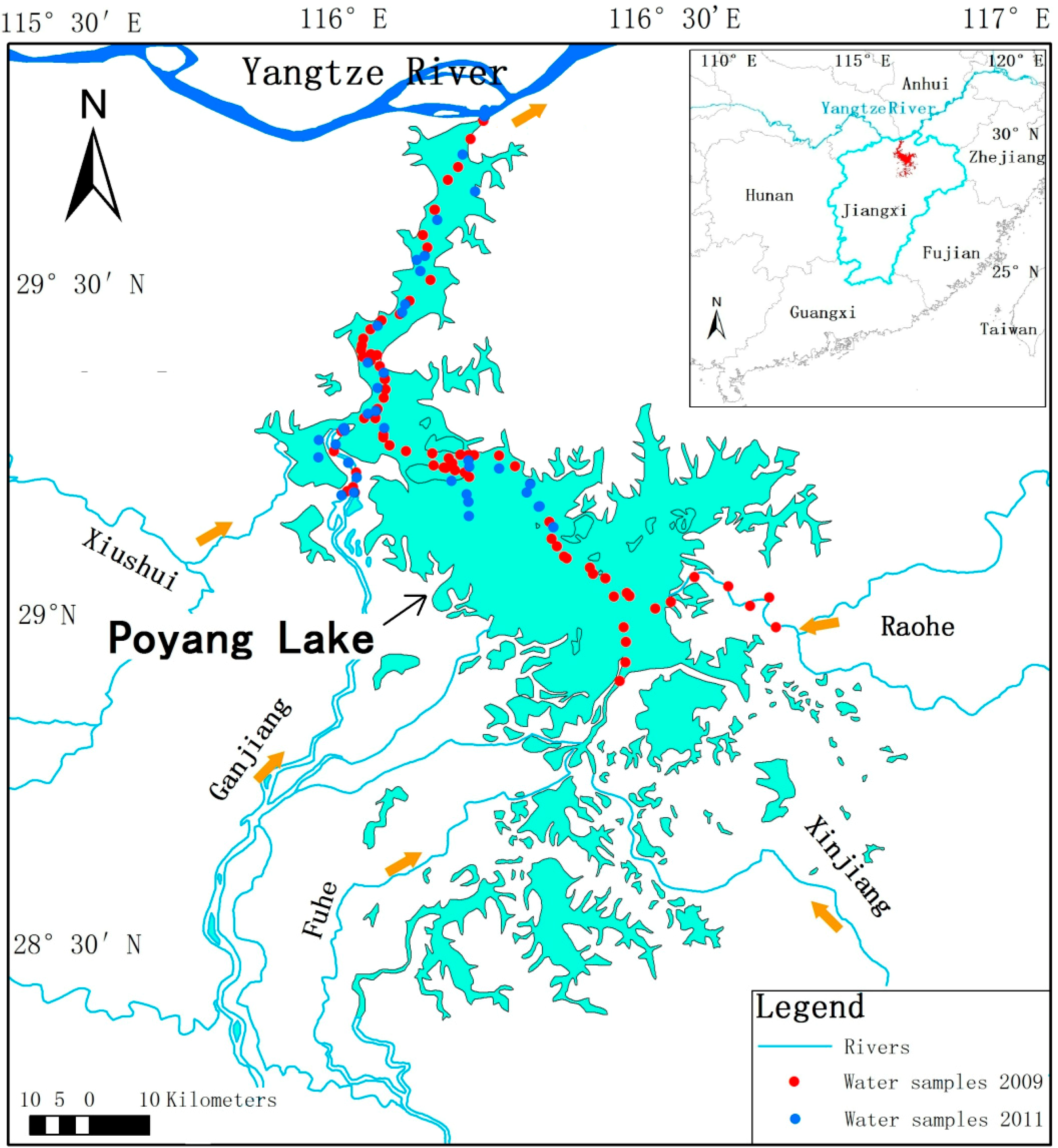
2. Study Area and Environmental Settings
3. Data and Methods
3.1. Remote Sensing Data
3.2. In Situ Measurements
- (1)
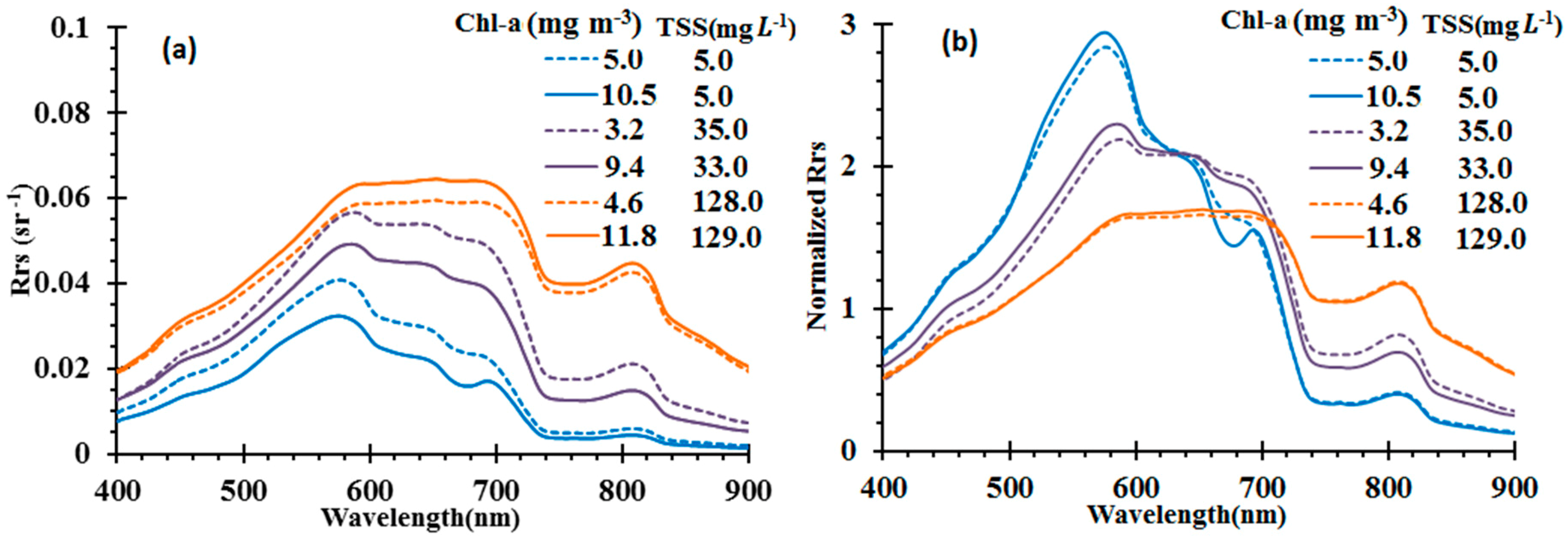
- ASD FieldSpec Pro FR2500 spectroradiometer (Analytical Spectral Devices, Inc., USA, 350 to 2500 nm with 4-nm increments) was used to measure the above-water hyperspectral remote sensing reflectance (Rrs, sr−1) following the NASA-recommended protocols [26]. All measurements were conducted from 10 am to 2 pm local time under clear sky conditions without apparent whitecaps or foam on the water surface. For each Rrs measurement, upward radiance (Lu), downward sky radiance (Lsky) and radiance from a standard Specrtralon reference plaque (Lplaque) were measured. Rrs was then derived as [26],where ρplaque is the reflectance of the reference plaque (~30%, provided by the manufacture) and ρf is the Fresnel reflectance of the water surface (assumed to be 0.022 for a calm water surface) [26]. Several examples of Rrs and their corresponding Chl-a and TSS values are presented in Figure 2a.
- (2)
- Chl-a concentration (in mg·m−3) was measured using an RF-5301 Fluorescent Spectrophotometer (Shimadzu, Kyoto, Japan), calibrated by the Chl-a standards manufactured by Sigma Chemical Co. (St. Louis, MO, USA). In short, water samples were filtered through 0.45-um Whatman cellulose acetate membranes and then immediately stored in liquid nitrogen. The filters were then soaked with acetone (90%) to extract the Chl-a pigment, and a centrifuge was used to increase the extraction efficiency. After storing at 0 °C for 24 h, Chl-a was determined by measuring the extracted pigment samples. The mean Chl-a concentration for all of the water samples was determined to be 4.9 ± 3.3 mg·m−g.
- (3)
- To measure TSS concentration (in mg·L−1), the water sample was filtered on a weighted Whatman cellulose acetate membrane filter. After drying in a 45 °C oven for 24 h, the filter was weighed again, and TSS was determined by the weight difference divided by the filtered water volume. An analytical balance with a precision of 0.01 mg was used to weigh the filters. Mean TSS for all samples was 88.6 ± 92.0 mg·L−1.
- (4)
- To measure the absorption of colored dissolved organic materials (CDOM), water samples were filtered through 0.2-µm Millipore membrane filters. Then, their absorbance was measured with an Ocean Optics HR2000 spectrometer, a PX-2 light source and a liquid waveguide capillary cell with 1-m optical path length. The absorbance data were then converted to the absorption coefficient as aCDOM(λ) = ACDOM(λ) × ln(10)/1.0(m). The mean aCDOM(λ) of all samples at 560 nm was determined to be 0.13 ± 0.07 m−1 [27].
3.3. Other Auxiliary Data
4. Algorithm Development
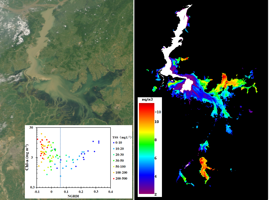
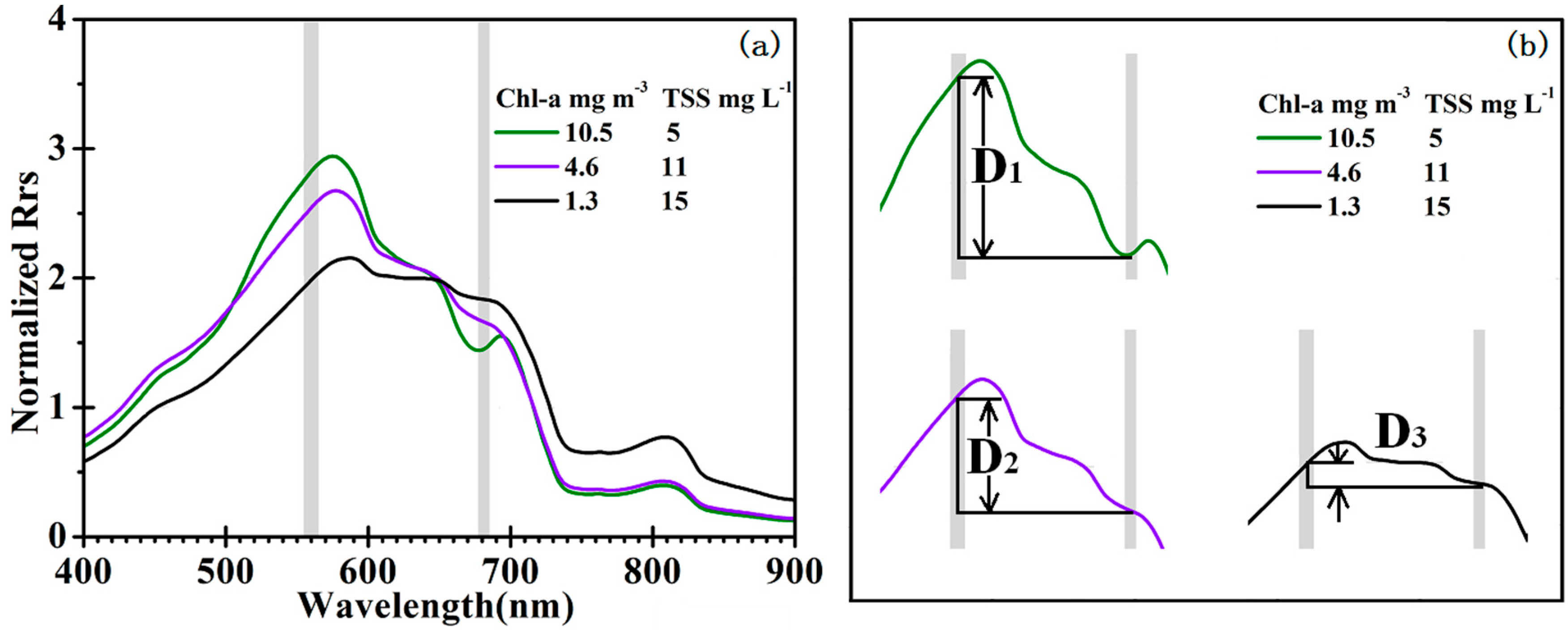
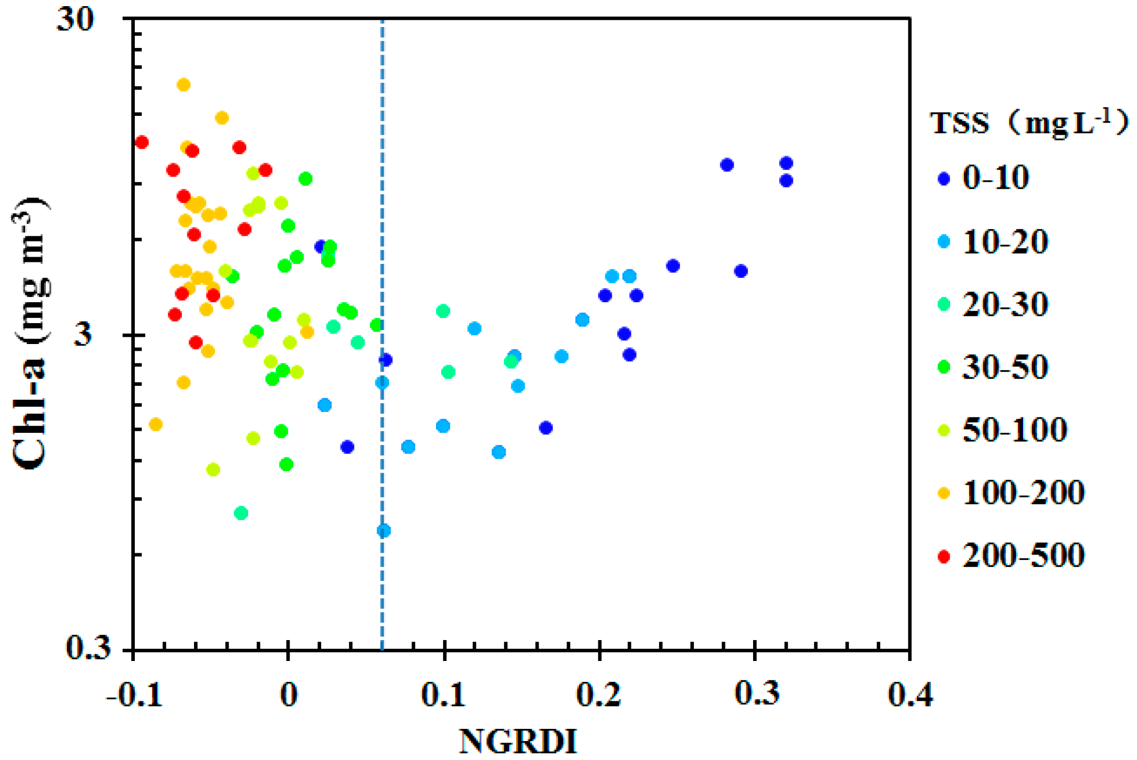
4.1. NGRDI-Based Algorithm


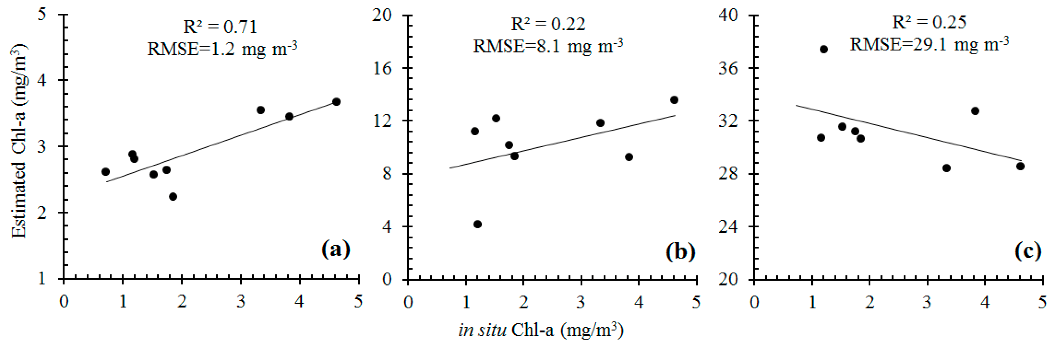
| NGRDI | Samples | Model | R2 | MRE (%) | RMSE (%) |
|---|---|---|---|---|---|
| >0.2 | 11 | y = 0.5892e8.6879x | 0.68 | 20.9 | 27.6 |
| >0.18 | 12 | y= 0.6309e8.4433x | 0.70 | 19.9 | 26.8 |
| >0.16 | 14 | y = 0.4623e9.5981x | 0.76 | 21.5 | 27.7 |
| >0.14 | 17 | y = 0.6048e8.5652x | 0.79 | 20.3 | 27.6 |
| >0.12 | 18 | y = 0.5284e9.094x | 0.81 | 21.5 | 28.0 |
| >0.10 | 20 | y = 0.756e7.639x | 0.73 | 24.8 | 32.3 |
| >0.07 | 23 | y = 0.874e7.0421x | 0.71 | 25.4 | 33.8 |
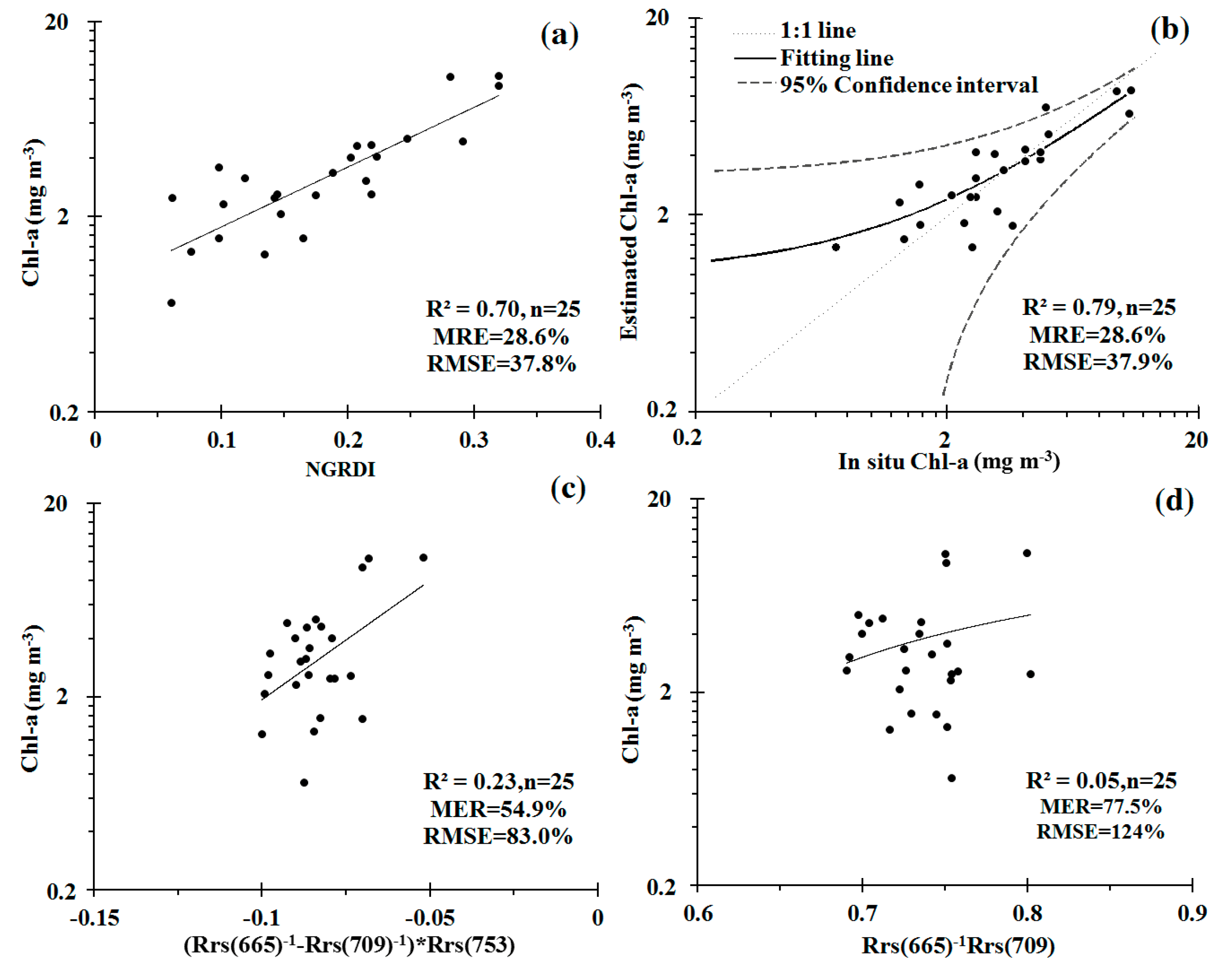
| >0.06 | 25 | y = 0.8724e7.0508x | 0.70 | 28.6 | 37.8 |
| >0.05 | 27 | y = 1.076e6.1187x | 0.62 | 32.2 | 43.0 |
| >0.04 | 28 | y = 1.1925e5.649x | 0.57 | 34.1 | 45.9 |
| >0.03 | 31 | y = 1.3058e5.2318x | 0.53 | 36.1 | 48.4 |
| >0.02 | 37 | y = 2.1724e2.8184x | 0.20 | 46.0 | 66.9 |
| >0 | 41 | y = 2.4048e2.3081x | 0.15 | 46.1 | 69.0 |

4.2. Application to MERIS Data

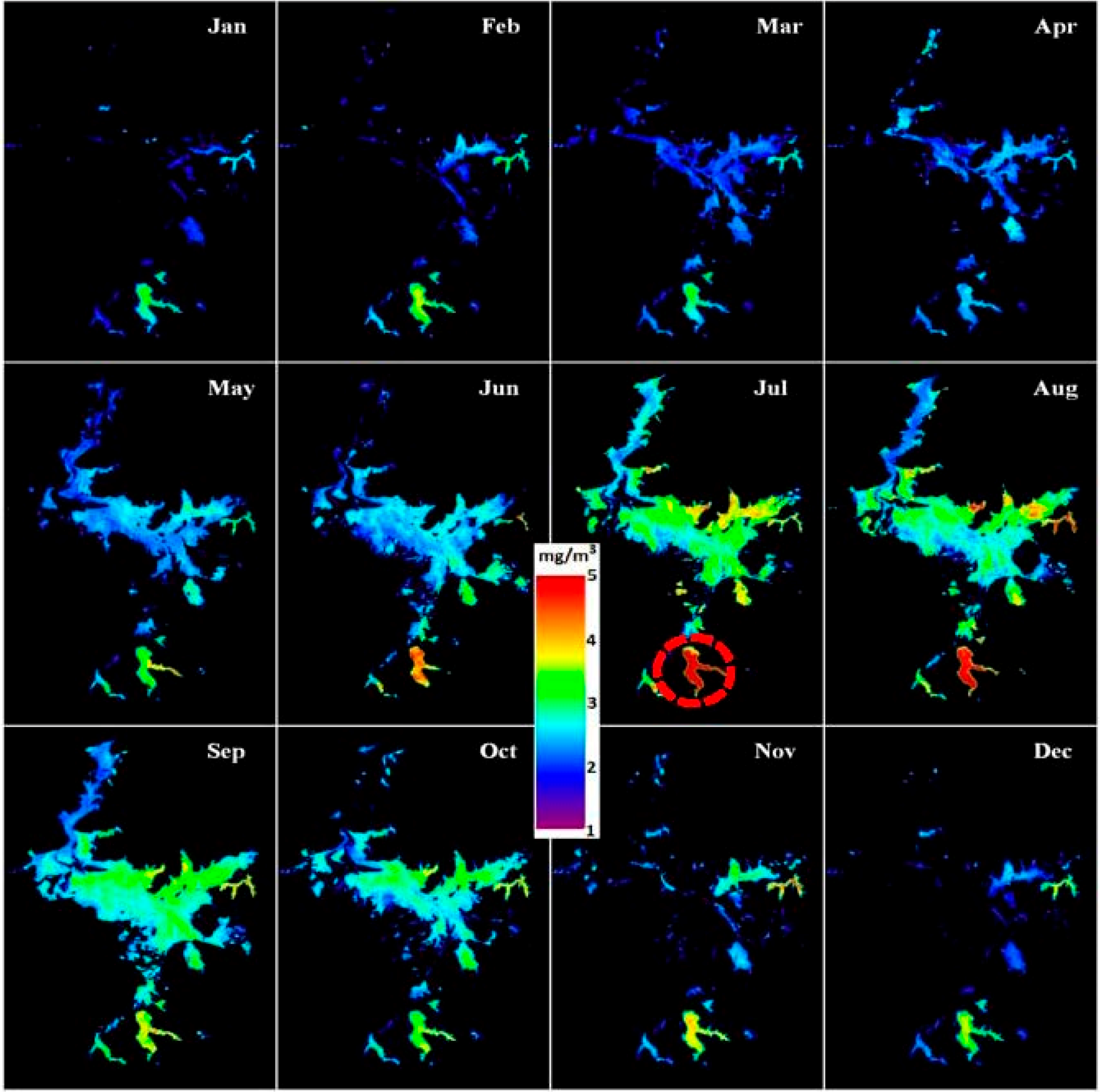
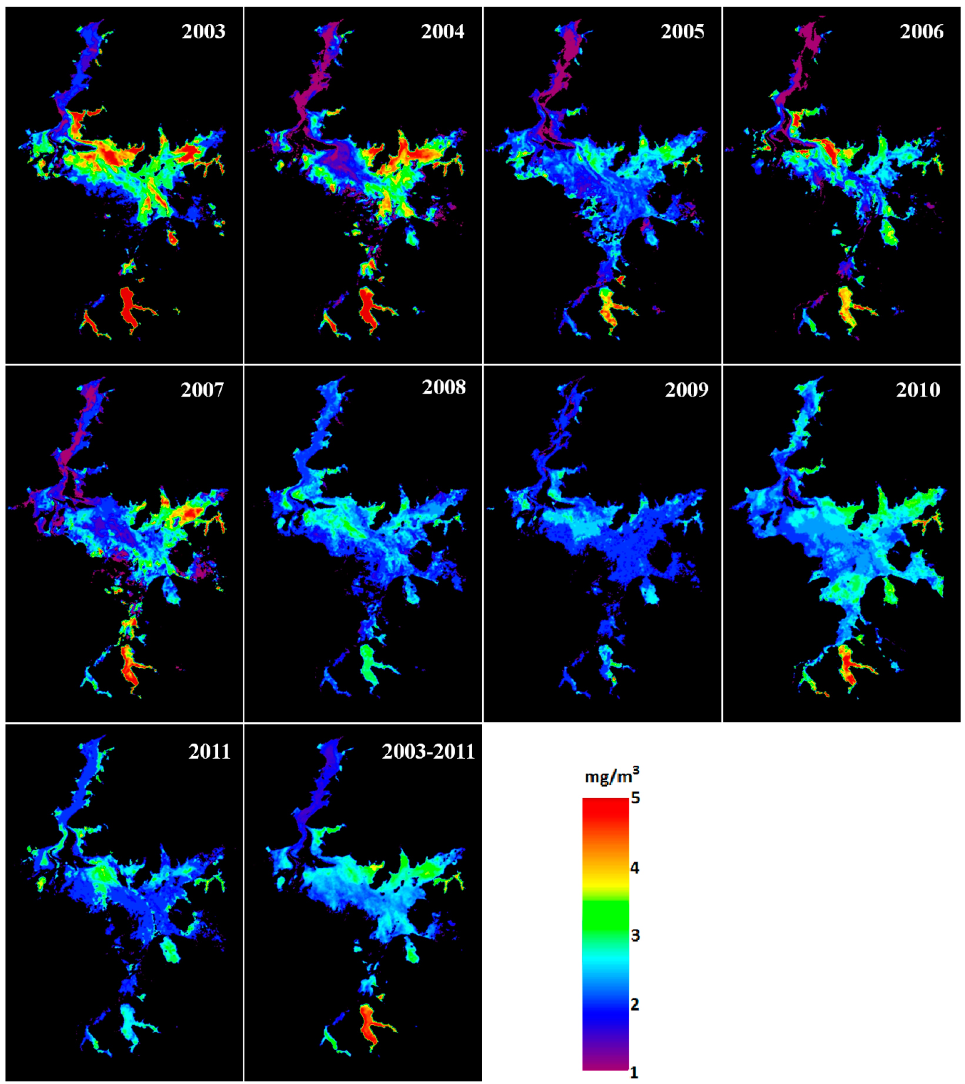
5. Seasonal and Inter-Annual Changes of Chl-a Concentrations

| Jan | Feb | Mar | Apr | May | Jun | Jul | Aug | Sep | Oct | Nov | Dec | Annual Mean | |
|---|---|---|---|---|---|---|---|---|---|---|---|---|---|
| Mean | 2.6 | 2.9 | 2.5 | 2.4 | 3.0 | 3.4 | 4.4 | 4.2 | 3.5 | 3.3 | 3.3 | 2.9 | 3.2 |
| Std. | 0.5 | 0.6 | 0.4 | 0.2 | 0.4 | 0.8 | 1.0 | 1.0 | 0.3 | 0.3 | 0.6 | 0.6 | 0.6 |


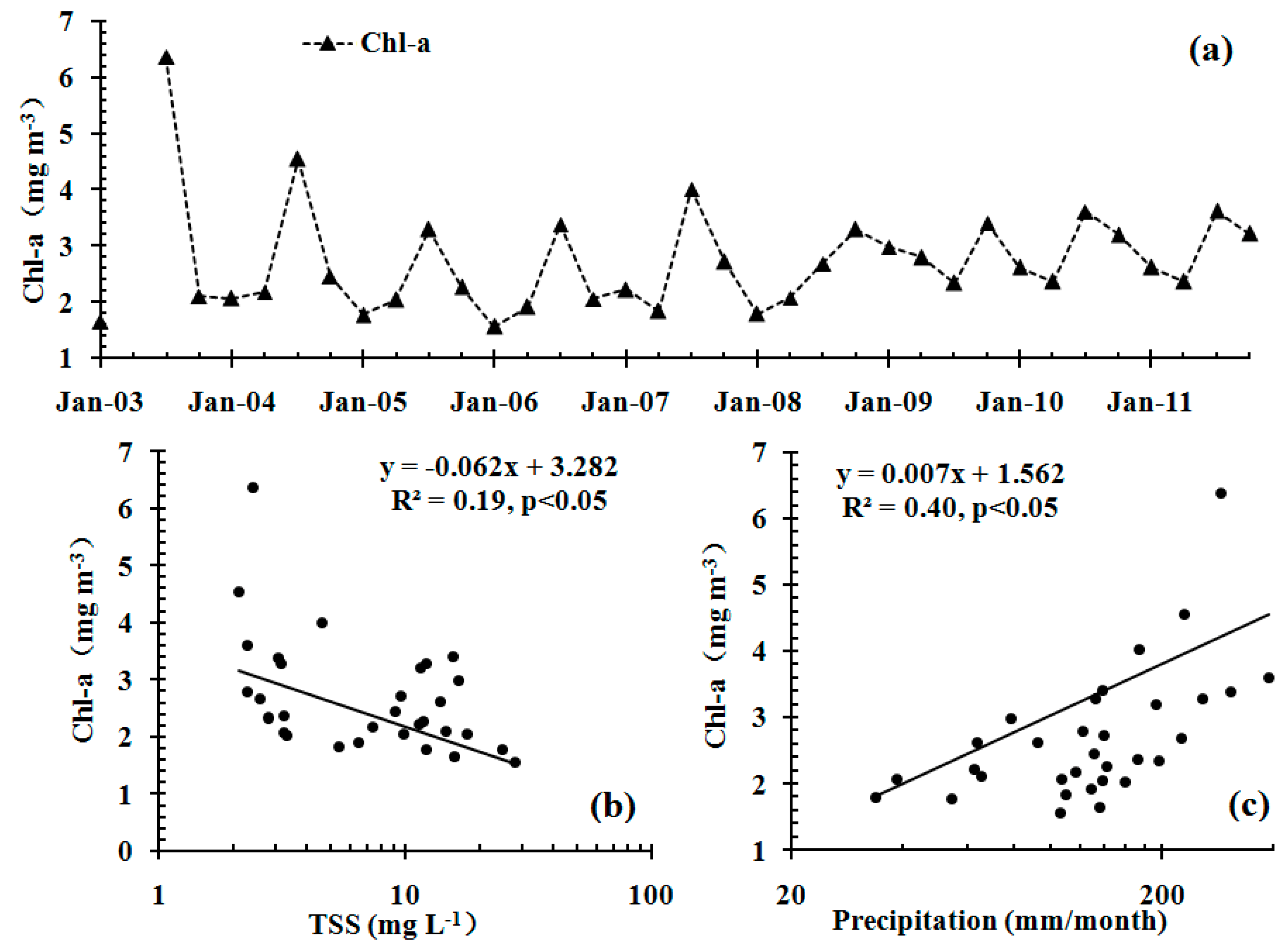
6. Driving Forces


7. Discussion
7.1. Validity of the Algorithm


7.2. Implications for Future Water Quality Management

8. Summary and Conclusions
Supplementary Files
Supplementary File 1Acknowledgements
Author Contributions
Conflicts of Interest
References
- Fang, J.; Rao, S.; Zhao, S. Human-induced long-term changes in the lakes of the Jianghan plain, central Yangtze. Front. Ecol. Environ. 2005, 3, 186–192. [Google Scholar] [CrossRef]
- Yang, G.; Ma, R.; Zhang, L.; Jiang, J.; Wei, S.; Zhang, M.; Zeng, H. Lake status, major problems and protection strategy in China. J. Lake Sci. 2010, 22, 799–810. [Google Scholar]
- Yin, L.; Jiang, N.; Yang, Y. Dynamic change of Lake Taihu area during the past 15 years based on remote sensing technique. J. Lake Sci. 2005, 17, 139–142. [Google Scholar]
- Hu, C.; Zhou, W.; Wang, M.; Wei, Z. Inorganic nitrogen and phosphate and potential eutrophication assessment in Lake Poyang. J. Lake Sci. 2010, 22, 723–728. [Google Scholar]
- Shang, G.P.; Shang, J.C. Causes and control countermeasures of eutrophication in Chaohu Lake, China. Chin. Geogr. Sci. 2005, 15, 348–354. [Google Scholar] [CrossRef]
- Feng, L.; Hu, C.; Chen, X.; Zhao, X. Dramatic inundation changes of China’s two largest freshwater lakes linked to the Three Gorges Dam. Environ. Sci. Technol. 2013, 47, 9628–9634. [Google Scholar] [CrossRef] [PubMed]
- Wu, G.; Leeuw, J.D.; Skidmore, A.K.; Prins, H.H.T.; Liuc, Y. Concurrent monitoring of vessels and water turbidity enhances the strength of evidence in remotely sensed dredging impact assessment. Water Res. 2007, 41, 3272–3280. [Google Scholar] [CrossRef]
- Wu, Z.; Cai, Y.; Liu, X.; Xu, C.P.; Chen, Y.; Zhang, L. Temporal and spatial variability of phytoplankton in Lake Poyang: The largest freshwater lake in China. J. Great Lakes Res. 2013, 39, 476–483. [Google Scholar] [CrossRef]
- Hu, C.; Feng, L.; Lee, Z.; Davis, C.O.; Mannino, A.; McClain, C.R.; Franz, B.A. Dynamic range and sensitivity requirements of satellite ocean color sensors: Learning from the past. Appl. Opt. 2012, 51, 6045–6062. [Google Scholar] [CrossRef] [PubMed]
- Adam, E.; Mutanga, O.; Rugege, D. Multispectral and hyperspectral remote sensing for identification and mapping of wetland vegetation: A review. Wetl. Ecol. Manag. 2010, 18, 281–296. [Google Scholar] [CrossRef]
- Ozesmi, S.L.; Bauer, M.E. Satellite remote sensing of wetlands. Wetl. Ecol. Manag. 2002, 10, 381–402. [Google Scholar] [CrossRef]
- Best, R.; Moore, D. Landsat interpretation of prairie lakes and wetlands of eastern south Dakota. In Proceedings of the Series-American Water Resources Association, New York, NY, USA, 26–27 September 1979.
- World Lake Database. Available online: Http://wldb.Ilec.Or.Jp/ (accessed on 9 October 2014).
- Zhang, B. Research of Poyang Lake; Shanghai Scientific & Technical Publishers: Shanghai, China, 1988. [Google Scholar]
- Feng, L.; Hu, C.; Chen, X.; Cai, X.; Tian, L.; Gan, W. Assessment of inundation changes of Poyang Lake using MODIS observations between 2000 and 2010. Remote Sens. Environ. 2012, 121, 80–92. [Google Scholar] [CrossRef]
- Shankman, D.; Keim, B.D.; Song, J. Flood frequency in China’s Poyang Lake region: Trends and teleconnections. Int. J. Climatol. 2006, 26, 1255–1266. [Google Scholar] [CrossRef]
- Zhong, Y.; Chen, S. Impact of dredging on fish in Poyang Lake. Jiangxi Fish. Sci. Technol. 2005, 1, 15–18. (In Chinese) [Google Scholar]
- Zhang, K. Poyang Lake: Saving the Finless Porpoise. Available online: http://www.chinadialogue.org.cn/article/show/single/en/839-Poyang-Lake-saving-the-finless-porpoise (accessed on 9 October 2014).
- Luo, D.; Wu, X.; Li, S.; Hu, C.; Zhou, W. Investigate study on tp pollution load of Poyang Lake by water and salt balance. J. Lake Sci. 2011, 47, 336–343. [Google Scholar]
- A 10 km-Long Cyanobacteria Bloom was Observed in Poyang Lake. Available online: http://www.Pyyou.Com/html/lvyouzixun/20121018/2485.Html (accessed on 9 October 2014). (In Chinese)
- Gordon, H.R. Atmospheric correction of ocean color imagery in the earth observing system era. J. Geophys. Res. 1997, 102, 17081–17106. [Google Scholar] [CrossRef]
- Gordon, H.R.; Wang, M. Retrieval of water-leaving radiance and aerosol optical thickness over the oceans with seawifs: A preliminary algorithm. Appl. Opt. 1994, 33, 443–452. [Google Scholar] [CrossRef] [PubMed]
- Bailey, S.W.; Franz, B.A.; Werdell, P.J. Estimation of near-infrared water-leaving reflectance for satellite ocean color data processing. Opt. Express 2010, 18, 7521–7527. [Google Scholar] [CrossRef] [PubMed]
- Hooker, S.; Firestone, E.R.; Patt, F.S.; Barnes, R.A.; Eplee, R.E., Jr.; Franz, B.A.; Robinson, W.D.; Feldman, G.C.; Bailey, S.W. Algorithm Updates for the Fourth Seawifs Data Reprocessing. Available online: http://oceancolor.gsfc.nasa.gov/SeaWiFS/TECH_REPORTS/PLVol22.pdf (accessed on 9 October 2014).
- Qi, L.; Hu, C.; Duan, H.; Cannizzaro, J.; Ma, R. A novel MERIS algorithm to derive cyanobacterial phycocyaninpigment concentrations in a eutrophic lake: Theoretical basis and practical considerations. Remote Sens. Environ. 2014, 154, 298–317. [Google Scholar] [CrossRef]
- Mobley, C.D. Estimation of the remote-sensing reflectance from above-surface measurements. Appl. Opt. 1999, 38, 7442–7455. [Google Scholar] [CrossRef] [PubMed]
- Yu, Z.; Chen, X.; Zhou, B.; Tian, L.; Yuan, X.; Feng, L. Assessment of total suspended sediment concentrations in Poyang Lake using HJ-1A/1B CCD imagery. Chin. J. Oceanol. Limnol. 2012, 30, 295–304. [Google Scholar] [CrossRef]
- Feng, L.; Hu, C.; Chen, X.; Tian, L.; Chen, L. Human induced turbidity changes in Poyang Lake between 2000 and 2010: Observations from MODIS. J. Geophys. Res. Ocean. (1978–2012) 2012, 117. [Google Scholar] [CrossRef]
- Gordon, H.R.; Morel, A.Y. Remote assessment of Ocean Color for Interpretation of Satellite Visible Imagery: A Review; American Geophysical Union: Washington, DC, USA, 1983. [Google Scholar]
- Morel, A.; Prieur, L. Analysis of variations in ocean color. Limnol. Oceanogr. 1977, 22, 709–722. [Google Scholar] [CrossRef]
- Knorn, J.; Rabe, A.; Radeloff, V.C.; Kuemmerle, T.; Kozak, J.; Hostert, P. Land cover mapping of large areas using chain classification of neighboring landsat satellite images. Remote Sens. Environ. 2009, 113, 957–964. [Google Scholar] [CrossRef]
- Babin, M.; Morel, A.; Fournier-Sicre, V.; Fell, F.; Stramski, D. Light scattering properties of marine particles in coastal and open ocean waters as related to the particle mass concentration. Limnol. Oceanogr. 2003, 48, 843–859. [Google Scholar] [CrossRef]
- Babin, M.; Stramski, D.; Ferrari, G.M.; Claustre, H.; Bricaud, A.; Obolensky, G.; Hoepffner, N. Variations in the light absorption coefficients of phytoplankton, nonalgal particles, and dissolved organic matter in coastal waters around Europe. J. Geophys. Res. 2003, 108. [Google Scholar] [CrossRef]
- Gurlin, D.; Gitelson, A.A.; Moses, W.J. Remote estimation of chl- a concentration in turbid productive waters—Return to a simple two-band NIR-red model? Remote Sens. Environ. 2011, 115, 3479–3490. [Google Scholar] [CrossRef]
- Gitelson, A.A.; Dall’Olmo, G.; Moses, W.; Rundquist, D.C.; Barrow, T.; Fisher, T.R.; Gurlin, D.; Holz, J. A simple semi-analytical model for remote estimation of chlorophyll-a in turbid waters: Validation. Remote Sens. Environ. 2008, 112, 3582–3593. [Google Scholar] [CrossRef]
- Efron, B. Estimating the error rate of a prediction rule: Improvement on cross-validation. J. Am. Stat. Assoc. 1983, 78, 316–331. [Google Scholar] [CrossRef]
- Hooker, S.B.; Esaias, W.E.; Feldman, G.C.; Gregg, W.W.; McClain, C.R. An Overview of Seawifs and Ocean Color; National Aeronautics and Space Administration, Goddard Space Flight Center: Greenbelt, MD, USA, 1992. [Google Scholar]
- Gregg, W.W.; Casey, N.W. Global and regional evaluation of the seawifs chlorophyll data set. Remote Sens. Environ. 2004, 93, 463–479. [Google Scholar] [CrossRef]
- Mishra, S.; Mishra, D.R. Normalized difference chlorophyll index: A novel model for remote estimation of chlorophyll-a concentration in turbid productive waters. Remote Sens. Environ. 2012, 117, 394–406. [Google Scholar] [CrossRef]
- Le, C.; Li, Y.; Zha, Y.; Sun, D.; Huang, C.; Lu, H. A four-band semi-analytical model for estimating chlorophyll a in highly turbid lakes: The case of Taihu Lake, China. Remote Sens. Environ. 2009, 113, 1175–1182. [Google Scholar] [CrossRef]
- Cheng, C.; Wei, Y.; Lv, G.; Yuan, Z. Remote estimation of chlorophyll-a concentration in turbid water using a spectral index: A case study in Taihu Lake, China. J. Appl. Remote Sens. 2013, 7. [Google Scholar] [CrossRef]
- Le, C.; Hu, C.; English, D.; Cannizzaro, J.; Kovach, C. Climate-driven chlorophyll-a changes in a turbid estuary: Observations from satellites and implications for management. Remote Sens. Environ. 2013, 130, 11–24. [Google Scholar] [CrossRef]
- Motohka, T.; Nasahara, K.N.; Oguma, H.; Tsuchida, S. Applicability of green-red vegetation index for remote sensing of vegetation phenology. Remote Sens. 2010, 2, 2369–2387. [Google Scholar] [CrossRef]
- Antoine, D.; Morel, A. A multiple scattering algorithm for atmospheric correction of remotely sensed ocean colour (MERIS instrument): Principle and implementation for atmospheres carrying various aerosols including absorbing ones. Int. J. Remote Sens. 1999, 20, 1875–1916. [Google Scholar] [CrossRef]
- Wang, M.; Shi, W. The NIR-SWIR combined atmospheric correction approach for MODIS ocean color data processing. Opt. Express 2007, 15, 15722–15733. [Google Scholar] [CrossRef] [PubMed]
- Doerffer, R.; Schiller, H. The MERIS case 2 water algorithm. Int. J. Remote Sens. 2007, 28, 517–535. [Google Scholar] [CrossRef]
- Baith, K.; Lindsay, R.; Fu, G.; McClain, C.R. Data analysis system developed for ocean color satellite sensors. Eos Trans. Am. Geophys. Union 2001, 82, 202–202. [Google Scholar] [CrossRef]
- Robinson, W.D.; Franz, B.A.; Patt, F.S.; Bailey, S.W.; Werdell, P.J. Masks and Flags Updates. Seawifs Postlaunch Technical Report Series. Available online: http://oceancolor.gsfc.nasa.gov/SeaWiFS/TECH_REPORTS/PLVol22.pdf (accessed on 9 October 2014).
- Feng, L.; Hu, C.; Chen, X.; Li, R.; Tian, L.; Murch, B. MODIS observations of the bottom topography and its inter-annual variability of Poyang Lake. Remote Sens. Environ. 2011, 115, 2729–2741. [Google Scholar] [CrossRef]
- Seip, K.L. Phosphorus and nitrogen limitation of algal biomass across trophic gradients. Aquat. Sci. 1994, 56, 16–28. [Google Scholar] [CrossRef]
- Teubner, K.; Dokulil, M.T. Ecological stoichiometry of TN: TP: SRSi in freshwaters: Nutrient ratios and seasonal shifts in phytoplankton assemblages. Arch. Fur Hydrobiol. 2002, 154, 625–646. [Google Scholar]
- Gons, H.J.; Rijkeboer, M.; Ruddick, K.G. A chlorophyll-retrieval algorithm for satellite imagery (medium resolution imaging spectrometer) of inland and coastal waters. J. Plankton Res. 2002, 24, 947–951. [Google Scholar] [CrossRef]
- Moses, W.J.; Gitelson, A.A.; Berdnikov, S.; Saprygin, V.; Povazhnyi, V. Operational MERIS-based nir-red algorithms for estimating chlorophyll-a concentrations in coastal waters—The Azov Sea case study. Remote Sens. Environ. 2012, 121, 118–124. [Google Scholar] [CrossRef]
- Hu, C.; Lee, Z.; Ma, R.; Yu, K.; Li, D.; Shang, S. Moderate resolution imaging spectroradiometer (MODIS) observations of cyanobacteria blooms in Taihu Lake, China. J. Geophys. Res. 2010, 115. [Google Scholar] [CrossRef]
- Gu., F.; Liu, W. Applications of remote sensing and gis to the assessment of riparian zones for environmental restoration in agricultural watersheds. Geo-Spat. Inf. Sci. 2010, 39, 386–389. [Google Scholar]
- Hu, C.; Le, C. Ocean color continuity from VIIRS measurements over Tampa Bay. IEEE Geosci. Remote Sens. Lett. 2014, 11, 945–949. [Google Scholar] [CrossRef]
- International Ocean Colour Science Meeting. 2015. Available online: http://iocs.Ioccg.Org/wp-content/uploads/1020-henri-laur-esa-from-meris-to-olci.Pdf (accessed on 9 October 2014).
© 2014 by the authors; licensee MDPI, Basel, Switzerland. This article is an open access article distributed under the terms and conditions of the Creative Commons Attribution license (http://creativecommons.org/licenses/by/4.0/).
Share and Cite
Feng, L.; Hu, C.; Han, X.; Chen, X.; Qi, L. Long-Term Distribution Patterns of Chlorophyll-a Concentration in China’s Largest Freshwater Lake: MERIS Full-Resolution Observations with a Practical Approach. Remote Sens. 2015, 7, 275-299. https://0-doi-org.brum.beds.ac.uk/10.3390/rs70100275
Feng L, Hu C, Han X, Chen X, Qi L. Long-Term Distribution Patterns of Chlorophyll-a Concentration in China’s Largest Freshwater Lake: MERIS Full-Resolution Observations with a Practical Approach. Remote Sensing. 2015; 7(1):275-299. https://0-doi-org.brum.beds.ac.uk/10.3390/rs70100275
Chicago/Turabian StyleFeng, Lian, Chuanmin Hu, Xingxing Han, Xiaoling Chen, and Lin Qi. 2015. "Long-Term Distribution Patterns of Chlorophyll-a Concentration in China’s Largest Freshwater Lake: MERIS Full-Resolution Observations with a Practical Approach" Remote Sensing 7, no. 1: 275-299. https://0-doi-org.brum.beds.ac.uk/10.3390/rs70100275